Wigner quantization of some one-dimensional Hamiltonians

G. Regniers †, and J. Van der Jeugt ‡

Department of Applied Mathematics and Computer Science, Ghent University,Krijgslaan 281-S9, B-9000 Gent, Belgium.

Short title: Wigner quantizationPACS numbers: 03.65.-w, 03.65.Fd, 02.20.Sv, 02.30.Gp

Abstract

Recently, several papers have been dedicated to the Wigner quantization of different Hamil-tonians. In these examples, many interesting mathematical and physical properties have beenshown. Among those we have the ubiquitous relation with Lie superalgebras and their repre-sentations. In this paper, we study two one-dimensional Hamiltonians for which the Wignerquantization is related with the orthosymplectic Lie superalgebra osp(1|2). One of them, theHamiltonian H = xp, is popular due to its connection with the Riemann zeros, discovered byBerry and Keating on the one hand and Connes on the other. The Hamiltonian of the free par-ticle, Hf = p2/2, is the second Hamiltonian we will examine. Wigner quantization introducesan extra representation parameter for both of these Hamiltonians. Canonical quantization isrecovered by restricting to a specific representation of the Lie superalgebra osp(1|2).

†E-mail: Gilles.Regniers@UGent.be‡E-mail: Joris.VanderJeugt@UGent.be

1

1 Introduction

Wigner quantization was initiated in 1950 by Eugene Wigner [1] and gained in interest by physicistsand mathematicians throughout the years. The principle of Wigner quantization is to dissociateoneself from the standard canonical commutation relations. In other words, for one-dimensionalsystems the canonical commutation relation

[x, p] = i~ (1)

no longer holds. Instead, the presupposed equivalence of Hamilton’s equations and the Heisenbergequations will relate the position operator x and the momentum operator p in a more general way.The result is a set of so-called compatibility conditions. From the validity of (1) one can deducethe compatibility conditions. In this sense, Wigner quantization is a more general approach thanthe widely known canonical quantization, where the canonical commutation relation (1) is assumedto be valid.

The compatibility conditions generally lead to triple relations containing commutators andanti-commutators. Only when the theory of Lie superalgebras was developed, it became clear thatthey are very useful in finding solutions for these triple relations. Therefore, the notion of Wignerquantum systems was only introduced much later than Wigner’s original paper, by Palev [2–4].

Wigner quantization has been studied extensively before [5–8]. The n-dimensional harmonicoscillator has proved to be fertile ground for investigation in Wigner quantization as well [9–13].As mentioned, the compatibility conditions can usually be rewritten as defining relations of a Liesuperalgebra. For example, the systems discussed in [14–16] have solutions related to gl(1|n) andosp(1|2n). In the present text, Wigner quantization of H = xp and Hf = p2/2 will lead to theLie superalgebra osp(1|2). If we want to determine the spectrum of these Hamiltonians, we muststudy the representations of osp(1|2). All irreducible ∗-representations of osp(1|2) are known andhave been classified in [17]. For the ∗-structure relevant in this paper, there appears to be only onesuch class of representations, the positive discrete series representations. They are characterizedby a positive parameter a. The specific value a = 1/2 will receive a lot of attention, as it representsthe canonical picture. In this way, we will be able to verify if our generalized results are consistentwith the known canonical case.

The paper is roughly divided in two big parts. In the first part we discuss the Wigner quanti-zation of a Hermitian operator corresponding to xp, namely Hb = (xp+ px)/2, and in the secondpart we handle the Hamiltonian of the free particle. At first sight it seems odd to deal with theless known Hamiltonian first. However, the calculations are more accessible for xp than for the freeparticle. Therefore, we treat the former, less difficult case in detail and we will be more succinctthroughout the second part of the paper.

In Section 2.1 we show how Wigner quantization of xp works and how it can be connected to theLie superalgebra osp(1|2). In order to know how Hb, x and p act as operators, we give a classificationof all irreducible ∗-representations of osp(1|2) in Section 2.2. At this point, we dispose of the actionsof all relevant operators in any representation of osp(1|2), so we could already compute the actionof Hb, x and p in order to find their spectrum. However, as it turns out these actions are relatedto certain orthogonal polynomials. Therefore, we first present some results on Meixner-Pollaczekpolynomials, Laguerre polynomials and generalized Hermite polynomials in Section 2.3. After this,we are able to determine the spectra of Hb, x and p in a standard way, shown in Section 2.4. Wethen compute the wave functions of the system in Section 2.5. Since Wigner quantization can beseen as a more general approach than canonical quantization, we can speak of generalized wavefunctions. Finally, we go back to the comfort zone of canonical quantization by taking a = 1/2.Our results prove to be compatible with what is known from the canonical setting.

2

The section concerning the free particle is roughly built up in the same way. However, thecomputations there are less detailed and the focus lies on the results.

2 The Berry-Keating-Connes Hamiltonian H = xp

The recent popularity of the Hamiltonian H = xpmust be attributed to its possible connection withthe Riemann hypothesis [18–20]. This conjecture states that the non-trivial zeros of the Riemannzeta function can all be written as 1/2+ itn, where the tn are real numbers. The first speculationsabout a potential relation between the Hamiltonian H and the Riemann zeros have been made in1999, by Berry and Keating on the one hand [21,22] and Connes on the other hand [23]. However,the idea of linking a certain Hamiltonian to the Riemann hypothesis is much older.The origin of this suggestion lies almost a century behind us, when Polya proposed that the imag-inary parts of the non-trivial Riemann zeros could correspond to the (real) eigenvalues of someself-adjoint operator. This statement is known as the Hilbert-Polya conjecture, although Hilbert’scontribution to this is unclear. For a long time the Hilbert-Polya conjecture was regarded as a boldspeculation, but it gained in credibility due to papers by Selberg [24] and Montgomery [25].The historical commotion around the Hamiltonian Hb = xp inspired us to perform the Wignerquantization of this one-dimensional system. As we shall see, a lot of interesting results emerge.

2.1 Wigner quantization and osp(1|2) solutions

In this section, we will perform the Wigner quantization of the Hamiltonian H = xp. The easiestHermitian operator corresponding to xp is

Hb =1

2(xp+ px). (2)

In the procedure of Wigner quantization, one starts from the operator form of Hamilton’s equationsand the equations of Heisenberg. The former take the explicit form

˙x =∂Hb

∂p= x, ˙p = −∂Hb

∂x= −p

and the equations of Heisenberg can be written as

˙x =i

~[Hb, x], ˙p =

i

~[Hb, p].

One then expresses the compatibility between these operator equations, thus creating a pair ofcompatibility conditions. For simplicity of notation, we set ~ = 1 and we find

[Hb, x] = −ix, [Hb, p] = ip,

or equivalently[{x, p}, x] = −2ix, [{x, p}, p] = 2ip, (3)

where {x, p} denotes the anticommutator between x and p: {x, p} = xp+ px.The goal is now to find Hilbert spaces in which the operators x and p act as self-adjoint operators

in such a way that they satisfy the compatibility conditions (3). In our future calculations, we arenot allowed to make any assumptions on the commutation relations between x and p. The readeris urged to verify that all these computations take this restriction into account. The strategy willbe to identify the algebra generated by x and p subject to (3). Since the relations (3) containanticommutators, Lie superalgebras come into the picture. In particular our problem will beconnected to osp(1|2) and representations of this Lie superalgebra will give us the demanded Hilbertspaces.

3

Proposition 1 The operators x and p, subject to the relations (3), generate the Lie superalgebra

osp(1|2).

Proof: Let us define new operators b+ and b−:

b± =x∓ ip√

2. (4)

These operators should satisfy (b±)† = b∓, where the dagger operation stands for the ordinaryHermitian conjugate. In terms of the b±, the operators Hb, x and p take the form

Hb =i

2

(

(b+)2 − (b−)2)

, x =b+ + b−√

2, p =

i(b+ − b−)√2

.

The compatibility conditions (3) are equivalent to the equations [Hb, b±] = −ib∓, which in turn

can be written as[(b−)2, b+] = 2b− and [(b+)2, b−] = −2b+,

using the previous expression of Hb in terms of b+ and b−. By writing down the commutators andanticommutators explicitly, one sees that the latter two relations are equivalent to

[

{b−, b+}, b±]

= ±2b±. (5)

These equations are known; they are the defining relations of the Lie superalgebra osp(1|2) [26].2

For now, we only need to know that osp(1|2) is generated by the odd elements b+ and b−,subject to the relations (5). The even elements of osp(1|2) are h, e and f , defined by

h =1

2{b+, b−}, e =

1

2(b+)2, f = −1

2(b−)2, (6)

satisfying the commutation relations

[h, e] = 2e, [h, f ] = −2f, [e, f ] = h.

If we regard the operators Hb, x and p as operators on a certain representation space of osp(1|2),we see that the Hamiltonian Hb is an even operator that can be written as

Hb = i(e+ f).

It is also clear that the position and momentum operators are odd operators on this representationspace.

We have now restated the crucial operators in terms of elements of the Lie superalgebra osp(1|2).One of our main objectives, however, is to determine the spectrum of the operators Hb, x and p.In order to achieve this goal, we need to have a Hilbert space in which we can determine howthe operators act. Lie superalgebra representations provide us with such a useful framework. Inparticular, we will work with irreducible ∗-representations of osp(1|2).

4

2.2 Irreducible ∗-representations of osp(1|2)The Z2-graded algebra osp(1|2), shortly described at the end of section 2.1 can be equipped witha so-called ∗-structure. This means that there exists an anti-linear anti-multiplicative involutionX 7→ X∗. So for X,Y ∈ osp(1|2) and a, b ∈ C we have that (aX + bY )∗ = aX∗ + bY ∗ and(XY )∗ = Y ∗X∗. In our case, this ∗-structure is provided by the action X 7→ X†. Restrictingthe ∗-structure to the even subalgebra of osp(1|2n) gives us the Lie algebra su(1, 1). So su(1, 1) isgenerated by h, e and f , defined in (6), which are related by the ∗-operation as follows:

h† = h, e† = −f, f † = −e.

We will be working with representations of ∗-algebras. If the inner product that is defined on therepresentation space satisfies

〈π(X)v, w〉 = 〈v, π(X∗)w〉 ,these representations are called ∗-representations. We emphasize that we choose this inner productto be antilinear in the first component. By doing so, we follow the convention accepted amongphysicists.All irreducible ∗-representations of osp(1|2) have been classified before. In 1981 this was done byHughes [27] using the shift operator technique, and much later by Regniers and Van der Jeugt [17]who also showed that two distinct classes of representations in [27] are in fact equivalent. Wesummarize the results of the latter reference in order to have a clear image of all irreducible∗-representations of osp(1|2). It turns out that there is only one such class of representationscompatible with the ∗-condition

(

b±)∗

= b∓, characterized by a positive parameter a. Theserepresentations ρa are called the positive discrete series representations and map the elements ofosp(1|2) to operators in ℓ2(Z+). The representation space V = ℓ2(Z+) is the Hilbert space ofall square summable complex sequences. It has standard basis vectors ek, (k = 0, 1, 2, . . .), whichare orthonormal with respect to the inner product on V . The parameter a characterizing therepresentation is defined by

ρa(h)e0 = ae0.

So e0 is assumed to be an eigenvector of ρa(h) with eigenvalue a. It is possible to show that, underthis assumption, the representation space V can be written as

V = V0 ⊕ V1.

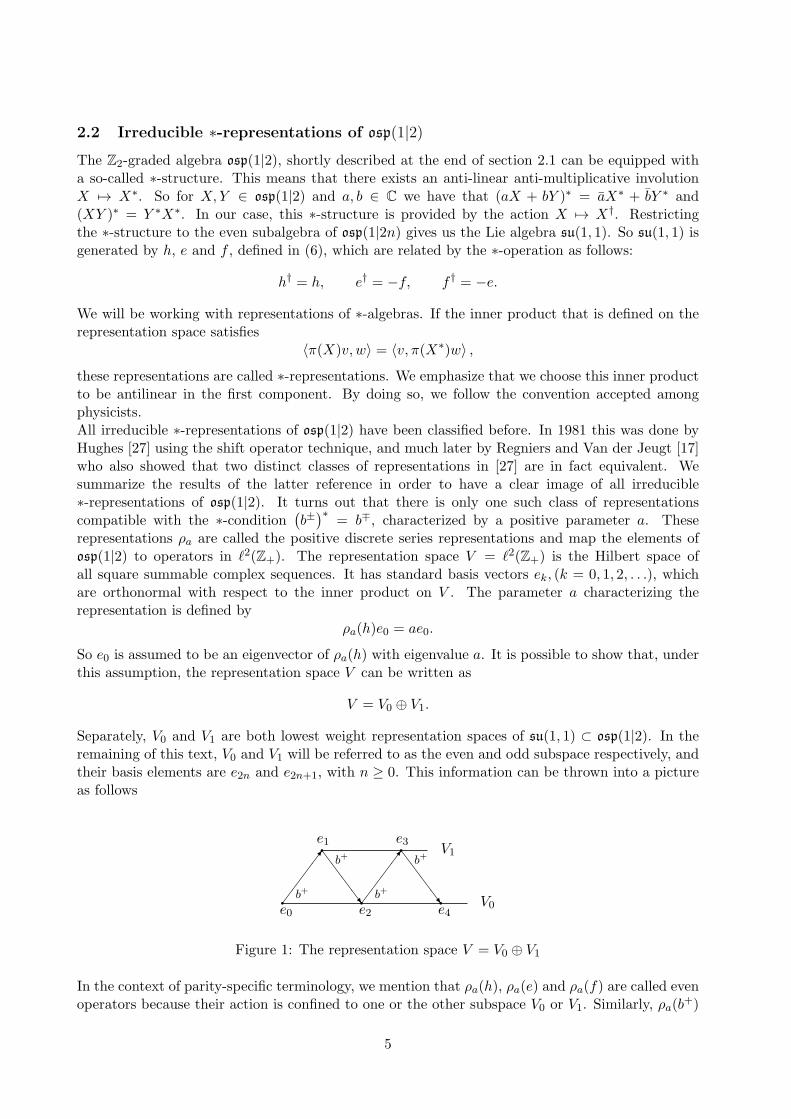
Separately, V0 and V1 are both lowest weight representation spaces of su(1, 1) ⊂ osp(1|2). In theremaining of this text, V0 and V1 will be referred to as the even and odd subspace respectively, andtheir basis elements are e2n and e2n+1, with n ≥ 0. This information can be thrown into a pictureas follows

V1

V0q q q

e0 e2 e4

q q

e1 e3

SSSSw

SSSSwb

+b+

����7

����7b

+b+

Figure 1: The representation space V = V0 ⊕ V1

In the context of parity-specific terminology, we mention that ρa(h), ρa(e) and ρa(f) are called evenoperators because their action is confined to one or the other subspace V0 or V1. Similarly, ρa(b

+)

5

and ρa(b−) are odd operators since they map from one subspace onto the other. This can be seen

in Figure 1. Such an intuitive picture is helpful in order to understand one of the main parts ofour paper: determining the spectrum of the operators Hb, x, p and later on Hf . For mathematicalarguments behind this classification, we refer to [17].Now the action of b+ and b− must be determined for both representation spaces separately. Weshall identify the representation space with an osp(1|2) module and write ρa(X)v = Xv from nowon. Then we have [17]

ρa(b+)e2n = b+e2n =

√

2(n+ a)e2n+1

ρa(b−)e2n = b−e2n =

√2n e2n−1

ρa(b+)e2n+1 = b+e2n+1 =

√

2(n+ 1)e2n+2

ρa(b−)e2n+1 = b−e2n+1 =

√

2(n+ a)e2n

(7)

We leave it to the reader to calculate the action of h, e and f on both subspaces with the help oftheir definitions (6). It is interesting to give the action of [x, p]:

[x, p] e2n = 2ai e2n, [x, p] e2n+1 = 2(1− a)i e2n+1.

We are left with the canonical commutation relation (1), for ~ = 1, when a takes the value 1/2.This is one way to see that this represents the canonical case.Now that we know the nature of the Hilbert spaces in which our operators act, we can try tofind eigenvectors of Hb, x and p. In section 2.4 we will see that these eigenvectors, and thus thespectrum of the respective operators, are related to orthogonal polynomials. Therefore, we need tointroduce the relevant orthogonal polynomials and some of their most interesting properties.

2.3 Some results on orthogonal polynomials

The most important formulas on all standard orthogonal polynomials are collected in the Askey-scheme [28, 29]. In this section, we will gather modifications and combinations of some formulasregarding the orthogonal polynomials that will arise in the following sections. The polynomialsin question are Meixner-Pollaczek polynomials, Laguerre polynomials and generalized Hermitepolynomials.

2.3.1 Meixner-Pollaczek polynomials

The classical Meixner-Pollaczek polynomials [28, 29] are defined by

P (λ)n (x;φ) =

(2λ)nn!

einφ 2F1

(−n, λ+ ix

2λ

∣

∣

∣

∣

1− e−2iφ

)

,

where 2F1 denotes the usual hypergeometric series and (a)n = a(a − 1) . . . (a − n + 1) is thePochhammer symbol. As all orthogonal polynomials, the Meixner-Pollaczek polynomials satisfya certain orthogonality relation and a three term recurrence relation. Both formulas are quite

involved and can be found in [28]. Instead, we will use the notation Pn(E) for P(a2)

n (E; π2 ), so wehave

Pn(E) = in(a)nn!

2F1

(−n, a2 + iE

a

∣

∣

∣

∣

2

)

.

For these specific polynomials, the orthogonality relation takes the form

1

2π

∫ +∞

−∞|Γ(a

2+ iE

)

|2Pm(E)Pn(E)dE =Γ(n+ a)

2a n!δmn, (8)

6

and the recurrence formula is

2E Pn(E) = (n+ a− 1)Pn−1(E) + (n+ 1)Pn+1(E).

We need a normalized version of the Meixner-Pollaczek polynomials, which we will denote by Pn(E):

Pn(E) =|Γ(a2 + iE)|

2

√

2a n!

π Γ(n+ a)Pn(E).

Actually, we should speak about the pseudo-normalized Meixner-Pollaczek functions. For reasonsthat will become clear later, we like them to satisfy the following orthogonality relation:

∫ +∞

−∞Pm(E) Pn(E)dE =

1

2δmn. (9)

Of course, the recurrence relation is also different for the Pn(E). It is given by

2E Pn(E) =√

n(n+ a− 1) Pn−1(E) +√

(n+ 1)(n+ a) Pn+1(E). (10)

This equation will come back in a different context in section 2.4.1.

2.3.2 Laguerre polynomials

Laguerre polynomials will only be important for the free particle, but since they are also needed todefine the generalized Hermite polynomials, we already summarize the main results for Laguerrepolynomials at this moment. The Laguerre polynomials [28, 29] are defined by

L(α)n (x) =

(α+ 1)nn!

1F1

( −nα+ 1

∣

∣

∣

∣

x

)

. (11)

The orthogonality of the Laguerre polynomials is expressed by

∫ ∞

0e−xxαL(α)

m (x)L(α)n (x)dx =

Γ(n+ α+ 1)

n!δmn, α > −1.

We define an altered version of these polynomials by

L(α)n (x) =

√2 e−

x2 x

α2

√

n!

Γ(n+ α+ 1)L(α)n (x).

Again, these polynomials are not really the normalized Laguerre polynomials. A factor of√2 is

added in order to obtain∫ ∞

0L(α)m (x) L(α)

n (x)dx = 2 δmn.

The three term recurrence relation of these functions can be written as

(2n− x+ α+ 1) L(α)n (x) =

√

n(n+ α) L(α)n−1(x) +

√

(n+ 1)(n+ α+ 1) L(α)n+1(x) (12)

and will be useful in the context of the free particle.

7

2.3.3 Generalized Hermite polynomials

The generalized Hermite polynomials Q(a)n (x) form the third family of orthogonal polynomials that

is of importance to us. They are not listed in the Askey-scheme, but they are closely related to the

Laguerre polynomials L(α)n (x), defined previously by equation (11). For positive n, the definition

of the generalized Hermite polynomials [30] is given by

Q(a)2n (x) = (−1)nL(a−1)

n (x2), Q(a)2n+1(x) = (−1)nxL(a)

n (x2).

The classical Hermite polynomials are found by choosing a = 1/2. As mentioned in the introduction,this is an important value for a. We will show how this indeed corresponds to the case of canonicalquantization. At this point however, the link with any type of quantization is not obvious at all,so let us not jump too far ahead.

Of course, there is also a set of orthogonality relations and a pair of recurrence relations forthe generalized Hermite polynomials. Instead of giving them here, we immediately define thenormalized version of these polynomials:

Q(a)2n (x) = |x|a− 1

2 e−x2

2

√

n!

Γ(n+ a)Q

(a)2n (x),

Q(a)2n+1(x) = |x|a− 1

2 e−x2

2

√

n!

Γ(n+ a+ 1)Q

(a)2n+1(x).

The functions Q(a)n (x) satisfy the following orthogonality relation:

∫ +∞

−∞Q(a)

m (x)Q(a)n (x)dx = δmn.

The pair of recurrence relations corresponding to the normalized generalized Hermite polynomials

Q(a)n (x) is given by

x Q(a)2n (x) =

√n Q

(a)2n−1(x) +

√n+ a Q

(a)2n+1(x),

x Q(a)2n+1(x) =

√n+ a Q

(a)2n (x) +

√n+ 1 Q

(a)2n+2(x).

(13)

Again, this recurrence relation is the primary result of this section because the same formulas willcharacterize different objects in section 2.4.2. We will then be able to identify these objects with

the normalized generalized Hermite polynomials Q(a)n (x).

2.4 Spectrum of the operators Hb, x and p

The first main goal of this paper is to determine the spectrum of the essential operators in theosp(1|2) representation space V = V0 ⊕ V1. The operators x and p have comparable expressionsin terms of osp(1|2) generators and can thus be handled in a similar way. The spectrum of Hb

on the other hand is an entirely different issue. Since Hb = i(e + f) is an even operator, usingthe terminology of section 2.2, the spectrum of Hb can be considered in both subspaces V0 or V1separately. The operator x is clearly an odd operator, so in this case one cannot look at bothsubspaces individually.Determining the spectrum of the operators Hb and x is done using the same method. One starts bydefining a formal eigenvector of Hb and x, with respective eigenvalues E and x. These eigenvectorsare unknown linear combinations of the basis vectors en of V . A three term recurrence relation forthe coefficients can then be calculated, and this will enable us to identify these coefficients with

8

orthogonal polynomials. From the spectral theorem for unbounded self-adjoint operators [31, 32]one can then derive that the spectrum of the operators is equal to the support of the weight functionof the corresponding orthogonal polynomials. It is then easy to find the spectrum of Hb and x.

2.4.1 Spectrum of Hb = i(e+ f)

For the spectrum of the Hamiltonian Hb, we start by defining a formal eigenvector u0(E), for theeigenvalue E:

u0(E) =∞∑

n=0

α2n(E)e2n, (14)

where α2n(E) are some unknown functions to be determined. We have already argued that thespectrum of Hb can by considered in both subspaces V0 and V1 separately. The vector u0(E) is anelement of the even subspace V0 and the action of Hb on this vector results in another element ofV0, as one sees from

Hb u0(E) =∞∑

n=0

α2n(E)(

i√

(n+ 1)(n+ a) e2n+2 − i√

n(n+ a− 1) e2n−2

)

.

This has been established by rewriting Hb = i(e+f) with the help of (6), which makes it possible touse equations (7) in order to determine the action of Hb on u0(E). We can try to find the unknowncoefficients α2n(E) by collecting the coefficients of e2n in the expression Hbu0(E) = Eu0(E). Weend up with the following recurrence relation:

E α2n = i√

n(n+ a− 1)α2n−2 − i√

(n+ 1)(n+ a)α2n+2.

We then define α2n(E) = (−i)nα2n(E), for which the recurrence relation reads

E α2n =√

n(n+ a− 1) α2n−2 +√

(n+ 1)(n+ a) α2n+2.

If we compare this with equation (10), we see that both formulas are almost the same. The unknownobjects α2n(E) can therefore be identified with the normalized Meixner-Pollaczek polynomials. Wehave

α2n(E) = Pn(E

2).

We have found the coefficients α2n(E) which determine the formal eigenvector (14). They can bewritten as

α2n(E) = (−1)n√

(a)nn!

A0(E) 2F1

(−n, a+iE2

a

∣

∣

∣

∣

2

)

, (15)

with

A0(E) =

∣

∣Γ(

a+iE2

)∣

∣

√

22−a π Γ(a).

So far, we have used the language of formal eigenvectors, but the result can also be formulated ina different mathematical way. Herein, Hb acts as a Jacobi operator on the basis {e2n|n ∈ Z+} ofV0 ∼= ℓ2(Z+). Next, one defines a map Λ from ℓ2(Z+) to square integrable functions L2(R, w(E)dE),where w(E) = |Γ(a2+iE)/2| is the weight function corresponding to Meixner-Pollaczek polynomials,by

(Λe2n)(E) = (−i)n√

2a n!

π Γ(n+ a)Pn(

E

2).

9

Then Λ ◦ Hb = ME ◦ Λ, i.e. Λ intertwines Hb acting in ℓ2(Z+) with the multiplication operatorME on L2(R, w(E)dE), see [33, Prop. 3.1]. Since we are really dealing with aspects of Wignerquantization in this paper, we shall not overload it with stricter terminology and just use the forphysicists more familiar language of formal eigenvectors, delta-functions, etc.

We can now rely on the spectral theorem to find the spectrum of Hb in V0: it is equal tothe support of the weight function of the Meixner-Pollaczek polynomials. This weight function,accompanying the polynomials under the integral in equation (8), has the real axis as its support.As a result, the spectrum of Hb in V0 is R.The same technique will give us the spectrum of Hb in V1. We start by defining a formal eigenvectoru1(E), determined by the coefficients α2n+1(E). These are then calculated in the same way as forthe coefficients α2n(E). The analysis and results can be copied exactly, but the parameter a hasto be changed into a+ 1. Thus we have

α2n+1(E) = (−1)n√

(a+ 1)nn!

A1(E) 2F1

(−n, a+1+iE2

a+ 1

∣

∣

∣

∣

2

)

, (16)

with

A1(E) =

∣

∣Γ(

a+1+iE2

)∣

∣

√

21−a π Γ(a+ 1).

The reason for this is that in V0 the lowest weight vector is e0 and h e0 = a e0 characterizes thisrepresentation. In V1 on the other hand, e1 is the lowest weight vector, and the correspondinglowest weight is a+ 1. The conclusion in this case is similar: the spectrum of Hb in V1 is R.Combining these results, we have:

Theorem 2 In the osp(1|2) representation space V , the Hamiltonian Hb has formal eigenvectors

u0(E) =∞∑

n=0

α2n(E)e2n,

with coefficients determined by equation (15), and

u1(E) =∞∑

n=0

α2n+1(E)e2n+1,

with coefficients (16). The spectrum of Hb in V is R with multiplicity 2.

It is important to note that the coefficients αn(E) have been chosen in such a way that the vectorsu0(E) and u1(E) are delta function normalized vectors. To support this statement, we first observethat

〈α2m(E), α2n(E)〉 =∫ +∞

−∞α∗2m(E)α2n(E) dE = δmn, (17)

which is a direct consequence of equation (9). We then multiply both sides of equation (14) byα∗2m(E) and integrate. With the help of equation (17) this yields

∫ +∞

−∞u0(E)α∗

2m(E) dE =

∞∑

n=0

e2n

∫ +∞

−∞α2n(E)α∗

2m(E) dE = e2m.

Now we have an integral expression for e2m, which is used to obtain

u0(E′) =

∞∑

m=0

a2m(E′)

∫ +∞

−∞u0(E)α∗

2m(E) dE

=

∫ +∞

−∞

( ∞∑

m=0

α2m(E′)α∗2m(E)

)

u0(E) dE.

10

The definition of the Dirac delta function implies that

∞∑

m=0

α∗2m(E)α2m(E′) = δ(E − E′).

From this, we can draw the immediate conclusion that u0(E) is a delta function normalized vector.Indeed:

⟨

u0(E), u0(E′)⟩

=∞∑

n=0

α∗2n(E)α2n(E

′) = δ(E − E′).

In an analogous way one can prove the same property for the vector u1(E), since equation (17) is alsovalid for odd indices. More generally, when a vector is decomposed in a certain orthonormal basis(in this case the osp(1|2) representation space basis en), and when the coordinates (the coefficientsαn(E)) are also orthonormal, then the vector is normalized with respect to the delta function. Wewill encounter this scenario for the eigenvectors of x, p and Hf .

2.4.2 Spectrum of x = (b++b−)√2

The spectrum of the operator x will be related to generalized Hermite polynomials, and the methodof reaching this relation is quite similar as before. The biggest difference is that we now have totake the entire representation space V into account. Thus, the formal eigenvector v(x) of x isdefined by

v(x) =∞∑

n=0

βn(x)en, (18)

satisfying the relation x v(x) = x v(x). The left hand side of this eigenvalue equation can be writtenas ∞

∑

n=0

β2n(√n e2n−1 +

√n+ a e2n+1) +

∞∑

n=0

β2n+1(√n+ a e2n +

√n+ 1 e2n+2),

using x = (b++b−)√2

together with equations (7). We can then compare the coefficients of en on both

sides of the equation, which will result in a pair of recurrence relations. We have

xβ2n =√nβ2n−1 +

√n+ a β2n+1,

x β2n+1 =√n+ a β2n +

√n+ 1β2n+2.

It should come as no surprise that we recognize the pair of recurrence relations (13) of the normalizedgeneralized Hermite polynomials. Therefore, we can identify the unknown coefficients βn(x) withthose polynomials:

βn(x) = Q(a)n (x).

The explicit expression for the β2n(x) is given by

β2n(x) = (−1)n√

(a)nn!

B0(x) 1F1

(−na

∣

∣

∣

∣

x2)

, (19)

with

B0(x) =|x|a−

12 e−

x2

2

√

Γ(a).

11

A similar expression describes the β’s with an odd index:

β2n+1(x) = (−1)n√

(a+ 1)nn!

B1(x) 1F1

( −na+ 1

∣

∣

∣

∣

x2)

, (20)

with

B1(x) =x |x|a−

12 e−

x2

2

√

Γ(a+ 1).

The same arguments as for the spectrum of Hb allow us to determine the spectrum of x. We have

Theorem 3 In the osp(1|2) representation space V , the position operator x has formal eigenvectors

v(x) =

∞∑

n=0

βn(x)en,

with coefficients determined by equations (19) and (20). The spectrum of x in V is equal to R,

which is the support of the weight function of the generalized Hermite polynomials.

Note that the major difference with Theorem 2 lies in the fact that the spectrum of the positionoperator does not have a double multiplicity. Each eigenvalue x belongs to exactly one eigenvectorv(x).

2.4.3 Spectrum of p = i(b+−b−)√2

Determining the spectrum of p is now just a formality because of the similar expressions for x andp. In fact, if we denote the formal eigenvector of p for the eigenvector p by

w(p) =∞∑

n=0

γn(p)en,

then it is not hard to see that the coefficients γn(p) can be written as

γn(p) = inβn(p),

where the βn(p) are given by equations (19) and (20). Thus, these coefficients are again generalizedHermite polynomials and we have

Theorem 4 In the osp(1|2) representation space V , the momentum operator p has formal eigen-

vectors

w(p) =∞∑

n=0

inβn(p)en,

with coefficients determined by equations (19) and (20). Just like x, p has a spectrum in V that is

equal to R.

As pointed out in section 2.4.1, the eigenvectors of x and p are normalized with respect to thedelta function. Thus we have

⟨

v(x), v(x′)⟩

= δ(x− x′)

and⟨

w(p), w(p′)⟩

= δ(p− p′),

ensuing from the fact that βn(x) and γn(p) are orthonormal functions.

12

2.5 Generalized wave functions

In the previous section we have constructed formal eigenvectors for all relevant operators Hb, x andp. Finding the wave functions corresponding to the physical states u0(E), u1(E), v(x) and w(p)requires the mutual inner products between these vectors. Therefore, we will compute these innerproducts before analyzing the wave functions explicitly.

2.5.1 Mutual inner products

This section is dedicated to the purely mathematical calculation of all inner products between thevectors u0(E), u1(E), v(x) and w(p). Two existing formulas will be crucial in these calculations.One of them is found in [34, Proposition 2] and states that

∞∑

n=0

(a)nn!

2F1

(−n, ba

∣

∣

∣

∣

y

)

1F1

(−na

∣

∣

∣

∣

x

)

tn

= (1− t)b−a(1− t+ yt)−b extt−1 1F1

(

b

a

∣

∣

∣

∣

xyt

(1− t)(1− t+ yt)

)

,

(21)

where |t| < 1. The other formula is the following approximation [35, equation (7.9)]:

limz→∞ 1F1

( c

a

∣

∣

∣z)

= limz→∞

Γ(a)

Γ(c)ez zc−a

∞∑

n=0

(a− c)n (1− c)nn!

z−n. (22)

These two equations will appear useful in the following.Let us first examine the inner products between the eigenvectors of x and Hb. We will only

calculate

〈v(x), u0(E)〉 =∞∑

n=0

α2n(E)β∗2n(x)

explicitly, since 〈v(x), u1(E)〉 is found in a highly similar way. The functions βn(x) are real, so thecomplex conjugation can be dropped. Using equations (15) and (19), we can write 〈v(x), u0(E)〉 as

A0(E)B0(x)∞∑

n=0

(a)nn!

2F1

(−n, a+iE2

a

∣

∣

∣

∣

2

)

1F1

(−na

∣

∣

∣

∣

x2)

.

In order to determine this summation, we need to add a factor tn to the nth summand and thentake the limit for t→ 1, with t < 1. Using equation (21), we rewrite

∑∞n=0 α2n(E)β2n(x)t

n as

A0(E)B0(x)(1− t)−a+iE

2 (1 + t)−a−iE

2 ex2tt−1 1F1

( a+iE2

a

∣

∣

∣

∣

2x2t

(1− t)(1 + t)

)

. (23)

The limit for t→ 1 is found with the help of equation (22). After simplification, we have

〈v(x), u0(E)〉 = A0(E)B0(x)Γ(a)

Γ(a+iE2 )

limt→1

ex2t1+t (|x|

√2t)−a+iE(1 + t)−iE

=

∣

∣Γ(a+iE2 )

∣

∣

Γ(a+iE2 )

|x|iE− 12

√π 2iE+2

(24)

= C0(E)|x|iE− 1

2

2√π

,

13

where |C0(E)|2 = 1. A similar derivation provides us with the inner product 〈v(x), u1(E)〉. It is

〈v(x), u1(E)〉 =∣

∣Γ(a+1+iE2 )

∣

∣

Γ(a+1+iE2 )

x |x|iE− 32

√π 2iE+2

(25)

= C1(E)x|x|iE− 3

2

2√π

,

where |C1(E)|2 = 1.We can deduce the inner products between the formal eigenvectors of p and Hb using (24) and

(25). First observe that

2F1

(

a, b

c

∣

∣

∣

∣

z

)

= (1− z)−a2F1

(

a, c− b

c

∣

∣

∣

∣

z

z − 1

)

,

together with A0(E) = A0(−E), implies that

(−1)nα2n(E) = α2n(−E).

A similar identity holds for odd indices of the coefficients αn(E): (−1)nα2n+1(E) = α2n+1(−E). Wehave used a standard hypergeometric identity that can be found in every book with an introductionto hypergeometric functions. We mention [29] as an example. It is then possible to see that

〈w(p), u0(E)〉 = 〈v(p), u0(−E)〉 (26)

and〈w(p), u1(E)〉 = −i 〈v(p), u1(−E)〉 , (27)

where the inner products with a vector v can be found in equations (24) and (25).What remains to be calculated is the inner product between the eigenvectors of the position

and momentum operators x and p. This inner product can be written as:

〈v(x), w(p)〉 =∞∑

n=0

inβn(x)βn(p),

which splits up as a sum over even indices and a sum over odd indices. Both series can be computedin an analogous fashion. For the even part we have

∞∑

n=0

(−1)nβ2n(x)β2n(p) = B0(x)B0(p)∞∑

n=0

(−1)n(a)nn!

1F1

(−na

∣

∣

∣

∣

x2)

1F1

(−na

∣

∣

∣

∣

p2)

. (28)

If we manage to write one of the 1F1-series as a 2F1 Gauss hypergeometric function, we can rely onequation (21) to simplify this equation. We shall make use of the following identity (see e.g. [28]):

limb→∞

2F1

(

a, b

c

∣

∣

∣

∣

z

b

)

= 1F1

( a

c

∣

∣

∣z)

. (29)

Applying this to 1F1

( −na

∣

∣x2)

, we see that the summation in the right-hand side of equation (28)can be calculated with the help of equation (21). After some simplifications, this summationtranslates to

2−aep2

2 limb→∞

(

b

b− x2

2

)b

1F1

(

b

a

∣

∣

∣

∣

x2p2

2(x2 − 2b)

)

.

14

Now the limit for b → ∞ can be taken for both factors. The first becomes ex2/2, while the second

is 0F1

( −a

∣

∣− x2p2/4)

. Putting all this together, we find that the even part of the inner product〈v(x), w(p)〉 is

∞∑

n=0

(−1)nβ2n(x)β2n(p) =|xp|a− 1

2

2a Γ(a)0F1

(−a

∣

∣

∣

∣

− x2p2

4

)

.

The odd part of the inner product is found in the same way, so we have

〈v(x), w(p)〉 = |xp|a− 12

2a Γ(a)

(

0F1

(−a

∣

∣

∣

∣

− x2p2

4

)

+ixp

2a0F1

( −a+ 1

∣

∣

∣

∣

− x2p2

4

))

. (30)

In the canonical case, many of these expressions simplify significantly. We discuss these simplifica-tions for a = 1/2 in section 2.5.2.

2.5.2 Generalized wave functions and the canonical case

Consider an arbitrary state of the system |ψ〉, written in Dirac’s bra-ket notation. Assume thatthe eigenstates of the position operator are denoted by |x〉. Then the spatial wave function of thesystem is found by

ψ(x) = 〈x|ψ〉 .Similarly, an inner product describes the wave function in the momentum space:

ψ(p) = 〈p|ψ〉 ,

where |p〉 represents the momentum eigenstates.We have written the position and momentum eigenvectors as v(x) and w(p) respectively. Their

inner product, given by equation (30), represents the wave function of the particle being locatedat position x, when the system is in the momentum eigenstate p. This result is compatible withthe canonical case where a = 1/2. In canonical quantization, x and p are known. The operator xis simply multiplication with x and p = −i∂x. For a = 1/2 equation (30) reduces to

〈v(x), w(p)〉 = 1√2Γ(12)

(

cos(xp) + i sin(xp))

=1√2π

eixp,

which is an eigenfunction of the canonical interpretation of the operator p with eigenvalue p.The case where the eigenstate |ψ〉 corresponds to the energy E needs to be handled with a little

more care, for there are two energy eigenstates corresponding to E. Both u0(E) and u1(E) belongto the same energy eigenvalue, thus inducing two independent wave functions ψ0

E(x) and ψ1E(x).

The previous results (24) and (25) allow us to write

ψ0E(x) = C0(E)

|x|iE− 12

2√π

(31)

and

ψ1E(x) = C1(E)

x|x|iE− 32

2√π

, (32)

with |C0|2 = |C1|2 = 1. Therefore the general wave function of the particle when the system’senergy equals E must be of the form

ψ(a)E (x) = Aψ0

E(x) +Bψ1E(x), (33)

15

with A and B complex coefficients satisfying |A|2 + |B|2 = 1. This result is compatible with the

canonical case as well, which is no surprise since ψ(a)E (x) is practically independent of a. In fact, in

equations (31) and (32) a only appears explicitly in the phase factors C0(E) and C1(E). For x = xand p = −i∂x, the Hamiltonian Hb converts into

Hb = −i(x∂x +1

2),

which, for a = 1/2, indeed has ψ0E(x) and ψ1

E(x) as eigenfunctions with eigenvalue E. Moreover,the general wave function (33) is normalized. We have (omitting the superscript (a) for clarity)

〈ψE′(x), ψE(x)〉 =∫ +∞

−∞ψ∗E′(x)ψE(x)dx = δ(E′ − E),

which follows from the well-known identity (for instance to be found in [36])

∫ +∞

−∞eik(x−x0)dk = 2π δ(x− x0).

In summary, we have

Theorem 5 In the Wigner quantization of the Hamiltonian Hb = xp, the wave function of the

particle with position coordinate x, when the total energy of the system equals E is given by

ψ(a)E (x) = A C0(E)

|x|iE− 12

2√π

+B C1(E)x|x|iE− 3

2

2√π

,

with |C0|2 = |C1|2 = 1 and |A|2 + |B|2 = 1.The wave function of the particle with position coordinate x, when the system’s momentum is equal

to p is given by

φ(a)p (x) =|xp|a− 1

2

2a Γ(a)

(

0F1

(−a

∣

∣

∣

∣

− x2p2

4

)

+ixp

2a0F1

( −a+ 1

∣

∣

∣

∣

− x2p2

4

))

.

Both results are compatible with the known expressions for these wave functions in canonical quan-

tization, which occurs when a = 1/2.

The wave function in the momentum basis is a superposition of two independent wave functionsdetermined by (26) and (27).

3 The Hamiltonian of the free particle Hf =12 p

2

Curiously, although many one-dimensional Hamiltonians have been studied before in the context ofWigner quantization, the simplest of them all had been forgotten until now. We choose to fill thislacuna next to the Berry-Keating-Connes Hamiltonian because, concerning Wigner quantization,there are a lot of similarities between Hb and the Hamiltonian of the free particle Hf . Since mostof the proofs and methods are very much alike, we will not mention any calculations unless theydiffer significantly from analogous computations in the previous section.

16

3.1 Relation with the osp(1|2) Lie superalgebra

The system of a particle having no potential energy, is described by the Hamiltonian

Hf =1

2p2, (34)

where p is the momentum operator of the particle. We note that the Hamiltonian is independentof the position operator x. Performing the Wigner quantization for the free particle starts withwriting down Hamilton’s equations and the equations of Heisenberg for this system. Hamilton’sequations give

˙p = −∂Hf

∂x= 0, ˙x =

∂Hf

∂p= p.

Together with the equations of Heisenberg (for ~ = 1)

[Hf , p] = −i ˙p, [Hf , x] = −i ˙x

we obtain a set of compatibility conditions

[Hf , p] = 0, [Hf , x] = −ip,

which is equivalent to[p2, x] = −2ip. (35)

Just as for the Berry-Keating-Connes Hamiltonian, the operators x and p subject to the currentcompatibility conditions (35) generate the Lie superalgebra osp(1|2). This is not so straightforwardto prove as before.

Theorem 6 If the operators x and p, subject to the relation [p2, x] = −2ip, are considered to be

odd elements of some superalgebra, then they must generate the Lie superalgebra osp(1|2).

Proof: We introduce the operators b+ and b− as before, see equation (4), by

b± =x∓ ip√

2.

The aim of this proof is to show that b+ and b− satisfy the defining relations (5) of osp(1|2):[

{b−, b+}, b±]

= ±2b±.

First we want to rewrite the compatibility conditions (35) in terms of b+ and b−. For thispurpose, we start by noticing that

[p2, b±] = b+ − b−. (36)

Either of these two relations can be fully rewritten in terms of b+ and b−. The result is the same,so let us focus on the commutator of p2 and b+. Substituting

p2 = −1

2

(

(b+)2 + (b−)2 − {b+, b−})

in this relation, we obtain

[{b+, b−}, b+]− [(b−)2, b+] = 2(b+ − b−).

Writing down the commutators and anticommutators explicitly, it is straightforward to see that

[(b−)2, b+] = −[{b+, b−}, b−],

17

so that finally both equations in (36) are equivalent to

[{b+, b−}, b+ + b−] = 2(b+ − b−). (37)

Next, assume that b+ and b− are odd elements of a Lie superalgebra L, that is b± ∈ L1, whereL1 is the odd part of the Lie superalgebra L = L0 ⊕L1. Anticommutators of the odd elements aresituated in the even part L0 of L. It is then necessary that the commutator of an odd and an evenelement must be an odd element again. Thus we can put

[{b+, b−}, b+] = −[(b+)2, b−] = Ab+ +Bb− (38)

for some constants A and B. The first equality again follows from explicit computation of thecommutators and anticommutators. With the help of equation (37) we then find:

[{b+, b−}, b−] = −[(b−)2, b+] = (−A+ 2)b+ − (B + 2)b−. (39)

We are able to determine the constants A and B by calculating [(b+)2, (b−)2] in two different ways.Indeed, from

[(b+)2, (b−)2] = b+[b+, (b−)2] + [b+, (b−)2]b+

= −2(A− 2)(b+)2 − (B + 2){b+, b−}

and

[(b+)2, (b−)2] = b−[(b+)2, b−] + [(b+)2, b−]b−

= −2B(b−)2 −A{b+, b−}

we can conclude that A = 2 and B = 0. Substituting this into (38) and (39), we obtain the osp(1|2)defining relations (5). 2

Thus, the operators x and p subject to the compatibility conditions (35), have solutions interms of osp(1|2) generators b+ and b−. Clearly x and p have the same expression as before, andthe Hamiltonian Hf can be written as

Hf = −1

4

(

(b+)2 + (b−)2 − {b+, b−})

Moreover, since x and p together with the compatibility conditions generate osp(1|2), no other Liesuperalgebra solutions exist.

3.2 Energy spectrum of the free particle

In this section, we will show that the spectrum of the Hamiltonian (34) is equal to R+ with double

multiplicity. The Hamiltonian of the free particle written in terms of the osp(1|2) generators b±

shows that Hf is an even operator in osp(1|2):

Hf = −1

2(e− f − h),

with h, e and f defined in equation (6). As we have already argued, an even operator can beregarded in both su(1, 1) subspaces V0 and V1 separately, which explains how we will end up witha double multiplicity in the energy spectrum.

18

Let z0(E) be a formal eigenvector of Hf with eigenvalue E in the subspace V0. We write thiseigenvector as

z0(E) =∞∑

n=0

ǫ2n(E)e2n,

where the ǫ2n(E) are coefficients we wish to determine. We can let Hf operate on this eigenvector,which gives

Hfz0(E) = −1

2

∞∑

n=0

ǫ2n(E)(√

(n+ 1)(n+ a) e2n+2 +√

n(n+ a− 1) e2n−2 − (2n+ a) e2n)

.

Since z0(E) is postulated to be an eigenvector of Hf with eigenvalue E, we also have

Hfz0(E) =∞∑

n=0

Eǫ2n(E)e2n.

Collecting the coefficients of e2n in both expressions for Hfz0(E), delivers us a three term recurrencerelation for the unknown functions ǫ2n(E):

(2n− 2E + a) ǫ2n =√

n(n+ a− 1) ǫ2n−2 +√

(n+ 1)(n+ a) ǫ2n+2.

This is recognized to be the recurrence relation (12) of the normalized Laguerre polynomials withα = a− 1 and x = 2E. So we can identify the ǫ2n(E) with these polynomials:

ǫ2n(E) = L(a−1)n (2E)

=

√

(a)nn!

E0(E) 1F1

(−na

∣

∣

∣

∣

2E

)

,

with

E0(E) =E

a−12 e−E

√2a

√

Γ(a).

Moreover, due to the chosen normalization we have∫ +∞

0ǫ2m(E)ǫ2n(E)dE = δmn.

The Laguerre polynomials have a weight function with a positive support, so the spectrum of Hf

in V0 is R+. In a similar way, one can define a formal eigenvector of Hf with eigenvalue E in V1:

z1(E) =

∞∑

n=0

ǫ2n+1(E)e2n+1.

The same procedure as before reveals that

ǫ2n+1(E) = L(a)n (2E)

=

√

(a+ 1)nn!

E1(E) 1F1

( −na+ 1

∣

∣

∣

∣

2t

)

,

with

E1(E) =E

a2 e−E

√2a+1

√

Γ(a+ 1).

Thus, we can conclude that the spectrum of Hf in V1 is also equal to R+. Combining both results,

we obtain

19

Theorem 7 The spectrum of Hf = −(e− f − h)/2 in the representation space V equals R+ with

multiplicity two.

Now that we have found the energy eigenstates of Hf , the corresponding wave function remainsto be sought. Crucial for this is the determination of some inner products.

3.3 Remaining inner products

Since 〈v(x), w(p)〉 is already known, the remaining inner products to be found are

〈v(x), z0(E)〉 , 〈v(x), z1(E)〉 , 〈w(p), z0(E)〉 and 〈w(p), z1(E)〉 .

The first two are rather straightforward, once the right identity is traced. In [37, equation (5.11.3.7)]we find

∞∑

n=0

(a)nn!

1F1

(−na

∣

∣

∣

∣

x

)

1F1

(−na

∣

∣

∣

∣

y

)

tn = (1− t)−a et(x+y)t−1 0F1

(−a

∣

∣

∣

∣

txy

(1− t)2

)

. (40)

The eigenvectors of x and Hf have an inner product that can be found by means of (40). We have

〈v(x), z0(E)〉 =∞∑

n=0

β2n(x) ǫ2n(E)

= B0(x)E0(E)∞∑

n=0

(−1)n(a)nn!

1F1

(−na

∣

∣

∣

∣

x2)

1F1

(−na

∣

∣

∣

∣

2E

)

.

Using (40) this simplifies to

〈v(x), z0(E)〉 = 1√2a Γ(a)

|x|a− 12 E

a−12 0F1

(−a

∣

∣

∣

∣

− 2E x2

4

)

. (41)

In a similar way, one obtains

〈v(x), z1(E)〉 = 1√2a+1 Γ(a+ 1)

x|x|a− 12 E

a2 0F1

( −a+ 1

∣

∣

∣

∣

− 2E x2

4

)

. (42)

The other pair of inner products is a harder nut to crack. We present the highlights of the com-putation. Omitting a factor of B0(p)E0(E), the calculation of the inner product 〈w(p), z0(E)〉 boilsdown to finding the summation

∞∑

n=0

(a)nn!

1F1

(−na

∣

∣

∣

∣

p2)

1F1

(−na

∣

∣

∣

∣

2E

)

. (43)

We apply equation (29) on the hypergeometric function with argument 2E, before using equations(21) and (22) to simplify the result. After a while, we obtain

Γ(a) p−2a limb→∞

1

Γ(b)

(

p2b

2E

)b

exp

(

p2(2E − b)

2E

)

.

For very large b, the Gamma-function can be written as√2π bb−1/2 exp(−b), so we can simplify

further to reachΓ(a)√

2p−2a exp(p2) lim

b→∞

√

b

πexp

(

b

[

1 + ln(p2

2E)− p2

2E

])

.

20

At this point, we can introduce the delta function by one of its limit definitions (see for instance [36])

δ(x) = limǫ→0+

1√πǫ

exp(−x2/ǫ).

Moreover, properties of the delta function allow us to write

δ

(√

p2

2E− ln(

p2

2E)− 1

)

= 2E√2 δ(p2 − 2E),

so that the summation (43) can be written as

Γ(a) e2E(2E)1−a δ(p2 − 2E).

Finding the desired inner product 〈w(p), z0(E)〉 requires adding a factor B0(p)E0(E) to the sum-mation (43). Simplifying once again finally gives

〈w(p), z0(E)〉 =√2√

|p| δ(p2 − 2E). (44)

Analogously, one finds

〈w(p), z1(E)〉 =√2

p√

|p|δ(p2 − 2E). (45)

At last we are ready to determine the generalized wave functions for the free particle and to compareour results with the canonical case.

3.4 Generalized wave function and the canonical case

The free particle has been thoroughly investigated in the past, which makes it easy to check ifour results are compatible with what is known. Luckily, they are. We have two wave functionsbelonging to the same energy eigenvalue E. In the position basis, we shall call them ψ0

E(x) andψ1E(x) and they are defined as the inner products (41) and (42) respectively. The general wave

function of the particle when the system’s energy equals E, written in the position basis must thenbe

ψ(a)E (x) = Aψ0

E(x) +Bψ1E(x), (46)

with A and B complex coefficients satisfying |A|2+ |B|2 = 1. This wave function is normalized withrespect to the delta function and it is compatible with the canonical case when a = 1/2. Indeed,for a = 1/2 equations (41) and (42) become

ψ0E(x) =

(2E)−14

√π

cos(x√2E)

and

ψ1E(x) =

(2E)−14

√π

sin(x√2E).

These are both eigenfunctions with eigenvalue E of the canonical interpretation of the HamiltonianHf = −∂2x/2. Note that, in the canonical case, the solution (46) is equivalent to

(

A− iB√2

)

(2E)−14

√2π

eix√2E +

(

A+ iB√2

)

(2E)−14

√2π

e−ix√2E ,

with |(A − iB)/√2|2 + |(A + iB)/

√2|2 = 1. This is the more traditional way of writing the

normalized wave function of the free particle, as a superposition of a plane wave moving to theright, and a plane wave going to the left. Note that this canonical notation for the wave functionis in accordance with the fact that the energy can be written as E = p2/2 in this case.

21

Theorem 8 In the Wigner quantization of the Hamiltonian Hf = p2

2 , the wave function of the

particle with position coordinate x, when the total energy of the system is equal to E is given by

ψ(a)E (x) =

A√2a Γ(a)

|x|a− 12 E

a−12 0F1

(−a

∣

∣

∣

∣

− 2E x2

4

)

+B√

2a+1 Γ(a+ 1)x|x|a− 1

2 Ea2 0F1

( −a+ 1

∣

∣

∣

∣

− 2E x2

4

)

,

with |A|2 + |B|2 = 1. This result is compatible with the known expression for this wave function in

canonical quantization, which occurs when a = 1/2.

In the momentum basis, the wave function is a superposition of the independent wave functionsdetermined by equations (44) and (45).

4 Conclusions

We have looked at the Wigner quantization of two different one-dimensional systems. The firstsystem is described by the Berry-Keating-Connes Hamiltonian H = xp and in the second part theHamiltonian of the free particle Hf = p2/2 is investigated.

Although both systems are entirely different, there are a lot of similarities in their Wignerquantization. Each time solutions for the compatibility conditions were found in terms of generatorsof the orthosymplectic Lie superalgebra osp(1|2). The actions of the operators x and p are thereforefound by looking at the positive discrete series representations of osp(1|2), which are characterizedby a parameter a. We find that the representation space on which all operators act, can be writtenas a direct sum V = V0 ⊕ V1. Both Hamiltonians also act on this Hilbert space, but their actionis confined to one of the two subspaces. The fact that these Hamiltonians have a spectrum withdouble multiplicity must be attributed to this observation, with the two subspaces V0 and V1 havingthe same structure.

Likewise, there are some differences to be found when looking at the two Hamiltonians. Thespectrum of the Berry-Keating-Connes Hamiltonian covers the entire real axis, while the spectrumof Hf only contains positive energy values. The reason for this is that the orthogonal polynomialsdescribing the energy eigenstates have a different support. The support of the weight functionof the Meixner-Pollaczek polynomials, appearing for H = xp equals R, while the weight functionof the Laguerre polynomials, related to the free particle system, has the positive real axis as itssupport.

The framework of Wigner quantization is less restrictive than canonical quantization. Therefore,generalized wave functions of the systems can be constructed. These wave functions, two for eachHamiltonian, are expected to be dependent on the representation parameter a. Remarkably, forH = xp this is not very much the case. Only the phase factors of the two independent wavefunctions contain a. In contrast with this, we find that the essential structure of the wave functionsfor the free particle is altered when a changes. Here, we have an actual generalization of thecanonical solution.

The latter remark suggests that one is able to retrieve the canonical case in some way. Indeed,one specific representation of osp(1|2) corresponds to the canonical picture. For each Hamiltonianwe find back the known canonical results for a = 1/2.

Acknowledgments

G. Regniers was supported by project P6/02 of the Interuniversity Attraction Poles Programme(Belgian State – Belgian Science Policy).

22

References

[1] E. P. Wigner, Phys. Rev. 77, 711-712 (1950).

[2] T.D. Palev, Czech J. Phys., Sect. B29, 91-98 (1979).

[3] T.D. Palev, J. Math. Phys. 23, 1778-1784 (1982).

[4] A.H. Kamupingene, T.D. Palev and S.P. Tsavena, J. Math. Phys. 27, 2067-2075 (1986).

[5] V.I. Man’ko, G. Marmo, E.C.G. Sudarshan and F. Zaccaria, Int. J. Mod. Phys., B11, 1281-1296 (1997).

[6] A. Horzela, Turk. J. Phys., 23, 903-910 (1999).

[7] A. Horzela, Czech J. Phys., 50, 1245-1250 (2000).

[8] E. Kapuscik, Czech J. Phys., 50, 1279-1282 (2000).

[9] T.D. Palev and N.I. Stoilova, J. Phys. A: Math. Gen. 27, 7387-7401 (1994).

[10] T.D. Palev and N.I. Stoilova, J. Math. Phys. 38, 2506-2523 (1997).

[11] R.C. King, T.D. Palev, N.I. Stoilova and J. Van der Jeugt, J. Phys. A: Math. Gen. 36, 4337-4362 (2003).

[12] R.C. King, T.D. Palev, N.I. Stoilova and J. Van der Jeugt, J. Phys. A: Math. Gen. 36, 11999-12019 (2003).

[13] T.D. Palev, SL(3|N) Wigner quantum oscillators: examples of ferromagnetic-like oscillators

with noncommutative, square-commutative geometry (2006), preprint hep-th/0601201.

[14] S. Lievens, N.I. Stoilova and J. Van der Jeugt, J. Math. Phys. 47, 113504 (2006).

[15] S. Lievens, N.I. Stoilova and J. Van der Jeugt, J. Math. Phys. 49, 073502 (2008).

[16] G. Regniers and J. Van der Jeugt, SIGMA 5, 106 (2009).

[17] G. Regniers and J. Van der Jeugt, In V. Dobrev, editor, Lie Theory and Its Applications

in Physics - VIII International Workshop, 138-147, AIP Conference Proceedings, Vol. 1243,2010.

[18] G. Sierra, J. Phys. A: Math. Theor. 41, 304041 (2008).

[19] H. C. Rosu, Mod. Phys. Lett. A 18, 1205-1213 (2003).

[20] B. Aneva, Phys. Lett. B 450, 388-396 (1999).

[21] M.V. Berry and J.P. Keating, Sel. Math. New ser. 5, 29-106 (1999).

[22] M.V. Berry and J.P. Keating, SIAM Rev. 41, 236-266 (1999).

[23] A. Connes, Sel. Math. New ser. 5, 29-106 (1999).

[24] A. Selberg, J. Indian Math. Soc. 20, 47-87 (1956).

[25] H. Montgomery, in: Analytic number theory, vol. 24, pp. 181-193 (Providence, RI, AmericanMathematical Society, 1973).

23

[26] Ganchev A.Ch., Palev T.D., A Lie superalgebraic interpretation of the para-Bose statistics, J.Math. Phys. 21 (1980), 797–799.

[27] J.W.B. Hughes, J. Math. Phys. 22 (2), 245-250 (1981).

[28] R. Koekoek and R.F. Swarttouw, The Askey-scheme of hypergeometric orthogonal polynomials

and its q-analogue, Technical Report 98–17, Delft University of Technology, 1998.

[29] R. Koekoek, P. A. Lesky and R. F. Swarttouw, Hypergeometric orthogonal polynomials and

their q-analogues, Springer-Verlag, 2010.

[30] T. S. Chihara, An introduction to orthogonal polynomials, Gorden and Breach, 1998.

[31] N. Dunford and J. T. Schwartz, Linear operators II: Spectral theory, self adjoint operators in

Hilbert space, Interscience publishers, New York, 1963.

[32] Yu. M. Berezanskiı, Expansions in eigenfunctions of selfadjoint operators, Providence (R.I.):American mathematical society, 1968.

[33] H.T. Koelink and J. Van der Jeugt, SIAM J. Math. Anal., 29, 794-822 (1998).

[34] J. Van der Jeugt and R. Jagannathan, J. Math. Phys. 39 (9), 5062-5078 (1998).

[35] N. M. Temme, Special functions: an introduction to the classical functions of mathematical

physics, Wiley, New York, 1996.

[36] C. Cohen-Tannoudji, B. Diu and F. Laloe, Quantum mechanics, Wiley, New York, 1977, Vol.2

[37] A.P. Prudnikov, Yu.A. Brychkov, O.I. Marichev, Integral and series, Gordon and BreachScience Publishers, 1986, Vol. 2

24