Wigner functions on non-standard symplecticvector spaces

Nuno Costa Dias∗ Joao Nuno Prata†

October 6, 2018

Abstract

We consider the Weyl quantization on a flat non-standard symplec-tic vector space. We focus mainly on the properties of the Wigner func-tions defined therein. In particular we show that the sets of Wignerfunctions on distinct symplectic spaces are different but have non-empty intersections. This extends previous results to arbitrary dimen-sion and arbitrary (constant) symplectic structure. As a by-productwe introduce and prove several concepts and results on non-standardsymplectic spaces which generalize those on the standard symplecticspace, namely the symplectic spectrum, Williamson’s theorem andNarcowich-Wigner spectra. We also show how Wigner functions onnon-standard symplectic spaces behave under the action of an arbi-trary linear coordinate transformation.

MSC [2000]: Primary 35S99, 35P05; Secondary 35S05, 47A75Keywords: Weyl quantization; Wigner functions; symplectic spaces; sym-

plectic spectrum; Williamson’s theorem; Narcowich-Wigner spectra

1 Introduction

In this work we return to the research programme initiated in [2, 3]. Therewe considered the Weyl-Wigner formulation of quantum mechanics based

∗ncdias@meo.pt†joao.prata@mail.telepac.pt

1

arX

iv:1

801.

0404

4v1

[m

ath-

ph]

12

Jan

2018

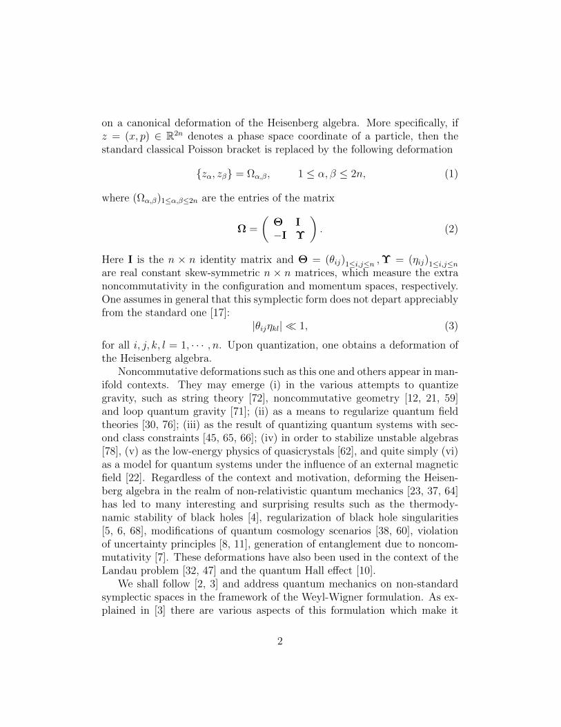
on a canonical deformation of the Heisenberg algebra. More specifically, ifz = (x, p) ∈ R2n denotes a phase space coordinate of a particle, then thestandard classical Poisson bracket is replaced by the following deformation

zα, zβ = Ωα,β, 1 ≤ α, β ≤ 2n, (1)

where (Ωα,β)1≤α,β≤2n are the entries of the matrix

Ω =

(Θ I−I Υ

). (2)

Here I is the n × n identity matrix and Θ = (θij)1≤i,j≤n ,Υ = (ηij)1≤i,j≤nare real constant skew-symmetric n × n matrices, which measure the extranoncommutativity in the configuration and momentum spaces, respectively.One assumes in general that this symplectic form does not depart appreciablyfrom the standard one [17]:

|θijηkl| 1, (3)

for all i, j, k, l = 1, · · · , n. Upon quantization, one obtains a deformation ofthe Heisenberg algebra.

Noncommutative deformations such as this one and others appear in man-ifold contexts. They may emerge (i) in the various attempts to quantizegravity, such as string theory [72], noncommutative geometry [12, 21, 59]and loop quantum gravity [71]; (ii) as a means to regularize quantum fieldtheories [30, 76]; (iii) as the result of quantizing quantum systems with sec-ond class constraints [45, 65, 66]; (iv) in order to stabilize unstable algebras[78], (v) as the low-energy physics of quasicrystals [62], and quite simply (vi)as a model for quantum systems under the influence of an external magneticfield [22]. Regardless of the context and motivation, deforming the Heisen-berg algebra in the realm of non-relativistic quantum mechanics [23, 37, 64]has led to many interesting and surprising results such as the thermody-namic stability of black holes [4], regularization of black hole singularities[5, 6, 68], modifications of quantum cosmology scenarios [38, 60], violationof uncertainty principles [8, 11], generation of entanglement due to noncom-mutativity [7]. These deformations have also been used in the context of theLandau problem [32, 47] and the quantum Hall effect [10].

We shall follow [2, 3] and address quantum mechanics on non-standardsymplectic spaces in the framework of the Weyl-Wigner formulation. As ex-plained in [3] there are various aspects of this formulation which make it

2

(in certain circumstances) more appealing than the ordinary formulation interms of operators acting on a Hilbert space. In the Weyl-Wigner repre-sentation one does not have to choose between a position or a momentumrepresentation of a state, as the Wigner function provides a joint distribu-tion of both. It is no surprise that the uncertainty principle and non-localitytake their toll on the Wigner function in the form of a lack of positivity[33, 48, 75]. Nevertheless, Wigner functions have positive marginals and per-mit an evaluation of expectation values of observables with the suggestiveformula

< A >=

∫R2n

a(z)Wρ(z)dz, (4)

where A is a self-adjoint operator, a is its Weyl symbol and Wρ is the Wignerfunction associated with some density matrix ρ. Moreover, the Weyl-Wignerframework is the only phase space formulation which is symplectically in-variant [26, 36, 40, 41, 42, 43, 54, 84]. More precisely, if Wρ(z) is a Wignerfunction and S is some symplectic matrix, then Wρ(Sz) is again a Wignerfunction. This makes it a privileged framework to study the semiclassicallimit of quantum mechanics [56, 61, 85]. The symplectic flavour of this ap-proach manifests itself equally in the dynamics of a quantum mechanicalsystem. The time evolution is governed by a quantum counterpart of thePoisson bracket - called Moyal bracket - which is a deformation of the Pois-son bracket [9, 34, 35, 53, 63, 77, 82]. From this perspective one sometimescalls this phase space formulation of quantum mechanics deformation quan-tization.

The Weyl-Wigner formulation is also particularly useful in the context ofquantum information with continuous variables [14, 74, 80].

For the quantization of systems with non-standard symplectic spaces, theadvantage of the Weyl-Wigner formulation becomes more emphatic. Thereason is that the Hilbert space for quantum mechanics on non-standardsymplectic spaces is still L2(Rn). So in the operator formulation, there is nodistinction between states for different symplectic structures. On the otherhand, in deformation quantization we proved in [2, 3] that the set of states(Wigner functions) in noncommutative quantum mechanics differs from theset of ordinary Wigner functions. We have used this fact as a criterionfor assessing when a transition from noncommutative to ordinary quantummechanics has taken place [29].

In [3] we considered the set FC of ordinary Wigner functions, the set FNC

3

of Wigner functions for the noncommutative symplectic structure (1,2), andthe set L of positive (classical) probability densities. We proved that in di-mension n = 2 any pair of these sets have non-empty intersections and noneof them contains the other. The main purpose of the present work is to gener-alize this result to arbitrary dimension n and to the sets Fω1 ,Fω2 of Wignerfunctions defined on the symplectic vector spaces (R2n;ω1), (R2n;ω2) withsymplectic forms ω2 6= ±ω1. Notice that the sympectic forms are completelyarbitrary (not necessarily of the form (2)), albeit constant.

As a byproduct we extend a number of definitions and results concerningordinary Wigner functions to Wigner functions on arbitrary, nonstandardsymplectic spaces. Moreover, as an application of our results, we solve theso-called representability problem in the case of linear coordinate transforma-tions. This terminology was coined in [20, 57] in the context of signal pro-cessing for pure states. Here we use the following definition for an arbitrary(pure or mixed) state. A given real and measurable phase-space functionF (z) is said to be representable if there exists a density matrix ρ such thatF is the Wigner function on some symplectic phase-space associated with ρ,i.e. F = Wρ. Here we consider linear coordinate transformations of the form

Wρ(z) 7→ (UMWρ)(z) = | detM |Wρ(Mz), (5)

with M ∈ Gl(2n;R). We then address the problem of the representability ofUMWρ.

Our results may also be potentially interesting for quantum informationof continuous variable systems. Indeed, the partial transpose - a linear coor-dinate transformation which has as sole effect the reversal of the momentumof one subsystem - is neither symplectic nor anti-symplectic [74, 80]. Hence,it maps a Wigner function on the standard symplectic vector space to aWigner function on a non-standard one. This transformation is used as acriterion to assess whether a state is separable or entangled.

Here is a summary of the main results of this work.

1) We define the notion of Narcowich-Wigner spectrum adapted to an arbi-trary symplectic form (Definition 5) and prove its main properties (Theorem10, Theorem 11).

2) We introduce the symplectic spectrum for an arbitrary symplectic form(Definition 15). We prove a Williamson-type theorem for non-standard sym-plectic spaces (Theorem 17) and show the usefulness of symplectic spectra

4

for generalized uncertainty principles (Theorem 19). In Theorem 23 we showthat we can always find a positive-definite matrix which has distinct symplec-tic spectra relative to two different symplectic forms. This result is fine-tunedfor the smallest symplectic eigenvalue in Theorem 24.

3) We solve the representability problem for linear coordinate transformationsin Theorems 25 and 28. In Theorem 25 we prove that UMWρ is representablefor any Wigner function Wρ if and only if M is symplectic or antisymplec-tic. Another new result is Theorem 28, which states that if M is neithersymplectic nor antisymplectic, then there exists a Wigner function Wρ suchthat UMWρ is again a Wigner function and Wρ′ for which UMWρ′ is not aWigner function.

4) Theorem 27 is one of the main results of this work and it shows that in thephase-space formulation different quantizations (i.e. on different symplecticspaces) yield different sets of states. However, there are always positivedistributions and states that are common to different quantizations. Theseresults are valid in arbitrary dimension and for arbitrary flat sympletic vectorspaces.

Notation

We denote by Pk×k(K) the convex cone of real (K = R) (or complex (K = C))symmetric (hermitean) positive (semi-definite) k × k matrices, and we writeP×k×k(K) if they are positive-definite. The set of real skew-symmetric k × kmatrices is A(k;R). The space of Schwartz test functions is denoted by S(Rn)and its dual S ′(Rn) are the tempered distributions. Latin indices i, j, k, · · · ,take values in the set 1, 2, · · · , n, whereas Greek indices α, β, γ, · · · arephase space indices which take values in 1, 2, · · · , 2n. The inner productin L2(Rn) is given by

< ψ|φ >=

∫Rnψ(x)φ(x)dx. (6)

We may at times write < ψ|φ >L2(Rn) and ||ψ||L2(Rn) for the correspond-ing norm if we want to emphasize that the functions are defined on then-dimensional Euclidean space Rn.

The Fourier-Plancherel transform for a function f ∈ L1(Rn) ∩ L2(Rn) is

5

defined by

(Ff)(ω) =

∫Rnf(x)e−ix·ωdx (7)

and its inverse is

(F−1f)(x) =1

(2π)n

∫Rnf(ω)eix·ωdω. (8)

In this work, we choose units such that Planck’s constant is h = 2π~ = 2π.

2 Symplectic vector spaces

Let V be some real 2n-dimensional vector space. A symplectic form on V is askew-symmetric non-degenerate bilinear form, that is a map ω : V × V → Rsuch that

ω(αx+ βy, z) = αω(x, z) + βω(y, z), ω(x, y) = −ω(y, x), (9)

for all x, y, z ∈ V and α, β ∈ R, and

ω(x, y) = 0, for all y ∈ V (10)

if and only if x = 0.The symplectic group Sp(V ;ω) is the group of linear automorphisms φ :

V → V such thatω (φ(z), φ(z′)) = ω(z, z′), (11)

for all z, z′ ∈ V . An automorphism φ is said to be anti-symplectic if

ω (φ(z), φ(z′)) = −ω(z, z′), (12)

for all z, z′ ∈ V . The archetypal symplectic vector space is V = R2n endowedwith the so-called standard symplectic form. As usual we write z = (x, p) ∈V = Rn× (Rn)∗ ' R2n, where x ∈ Rn is interpreted as the particle’s positionand p ∈ (Rn)∗ as the particle’s momentum belonging to the cotangent bundle.The standard symplectic form reads

σ(z, z′) = z · J−1z′ = p · x′ − x · p′, (13)

6

where z = (x, p), z′ = (x′, p′) and J = −J−1 = −JT is the 2n× 2n standardsymplectic matrix

J =

(0 I−I 0

). (14)

The symplectic group Sp(R2n;σ) ≡ Sp(n;σ) is then the set of matrices Psuch that

PJPT = J. (15)

We remark that if P ∈ Sp(n;σ), then also P−1,PT ∈ Sp(n;σ).A matrix A is σ-anti-symplectic [26] if

AJAT = −J. (16)

All σ-anti-symplectic matrices A can be written as

A = RP, (17)

where P ∈ Sp(n;σ) and

R =

(I 00 −I

). (18)

Thus a σ-anti-symplectic transformation is a σ-symplectic transformationfollowed by a reflection of the particle’s momentum.

More generally, for any other symplectic form on R2n, there exists a realskew-symmetric matrix Ω ∈ Gl(2n) such that

ω(z, z′) = z ·Ω−1z′, z, z′ ∈ R2n. (19)

A well known theorem in symplectic geometry [16, 40] states that all sym-plectic vector spaces of equal dimension are symplectomorphic. In otherwords, if (V, ω) and (V ′, ω′) have the same dimension, then there exists alinear isomorphism φ : V → V ′ such that

φ∗ω′ = ω. (20)

Here φ∗ denotes the pull-back of φ. In particular, (R2n, σ) is symplectomor-phic with (R2n, ω) for any symplectic form (19). So if φ : (R2n, σ)→ (R2n, ω)is given by

φ(z) = Sz, (21)

7

for some S ∈ Gl(2n), then we have from (20) that

φ∗ω = σ ⇔ ω(Sz,Sz′) = σ(z, z′), (22)

for all z, z′ ∈ R2n. And thus

Ω = SJST. (23)

The matrix S in (23) is not unique. Indeed, we have

Lemma 1 Suppose that S is a solution of (23). Then S′ is also a solutionif and only if S′−1S,S−1S′ ∈ Sp(n;σ).

Proof. We have Ω = SJST = S′JS′T if and only if S′−1SJ(S′−1S)T =S−1S′J(S−1S′)T = J.

We denote by D(n;ω) the set of all real 2n× 2n matrices satisfying (23)and call them Darboux matrices. The corresponding symplectic automor-phism (21) is called a Darboux map.

A matrix M is ω-symplectic if

MΩMT = Ω, (24)

and it is ω-anti-symplectic if

MΩMT = −Ω. (25)

Any ω-symplectic (resp. ω-anti-symplectic) matrix M is of the form

M = SPS−1, (26)

where S ∈ D(n;ω) and P is a σ-symplectic (resp. σ-anti-symplectic) matrix.For future reference we consider the following Proposition.

Proposition 2 Let η be an arbitrary symplectic form on R2n such that

|η(z, z′)| ≤ |σ(z, z′)|, (27)

for all z, z′ ∈ R2n. Then, there exists a constant 0 < |a| ≤ 1 such that

η = aσ. (28)

8

Proof. Let η(z, z′) = zTΣ−1z′ for z, z′ ∈ R2n and Σ ∈ Gl(2n;R). Letδα1≤α≤2n denote the canonical basis of R2n. If we set z = δα and z′ = δβin (27), we obtain:

|Σ−1αβ | ≤ |Jαβ|, (29)

for all 1 ≤ α, β ≤ 2n. So Σ−1αβ = 0, whenever Jαβ = 0. And so Σ−1 must be

of the form

Σ−1 =

(0 D−D 0

), (30)

where D = diag(µ1, · · · , µn). Next set z = δi − δj and z′ = δn+i + δn+j, for1 ≤ i < j ≤ n. A simple calculation shows that

σ(z, z′) = 0, η(z, z′) = µi − µj. (31)

But from (27) it follows that µi = µj for all 1 ≤ i < j ≤ n. And sothere exists a 6= 0 such that (28) holds. But again from (27), we must have0 < |a| ≤ 1.

3 Weyl Quantization

3.1 Weyl quantization on (R2n;σ)

One of the basic ingredients for the quantization of a classical system definedon the standard symplectic vector space (R2n;σ) is the Heisenberg-Weyl al-gebra: [

Zα, Zβ

]= iJαβ I ,

[Zα, I

]= 0, α, β = 1, · · · , 2n, (32)

where Z = (q, p) are the quantum-mechanical counterparts of the classical

phase-space variables z = (x, p) and I is the identity operator. Their actionon functions in their (densely defined) domains in L2(Rn) is given by

(Iψ)(x) = ψ(x), (qiψ)(x) = xiψ(x), (pjψ)(x) = −i∂jψ(x), (33)

for i, j = 1, · · · , n. These operators are not bounded, which prevents theconstruction of a C∗-algebra of observables. A familiar way to circumventthis is to consider the alternative algebra of Heisenberg-Weyl displacementoperators:

Dσ(ξ) = eiσ(ξ,Z). (34)

9

The action of Dσ(ξ) on ψ ∈ S(Rn) is given by the explicit formula

Dσ(ξ)ψ(x) = eip0·x−i2p0·x0ψ(x− x0), (35)

for ξ = (x0, p0). This extends to a unitary operator from L2(Rn) to L2(Rn)and to a continuous operator from S ′(Rn) to S ′(Rn).

Their commutation relations are easily established from (35) or, heuris-tically, from (32,34) using the Baker-Campbell-Hausdorff formula:

Dσ(ξ)Dσ(ζ) = ei2σ(ξ,ζ)Dσ(ξ + ζ) = eiσ(ξ,ζ)Dσ(ζ)Dσ(ξ), (36)

for ξ, ζ ∈ R2n. Operators of the form

Uσ(ξ, τ) = eiτDσ(ξ) (37)

constitute an irreducible unitary representation of the Heisenberg group H(n)of elements (ξ, τ) ∈ R2n × R with group multiplication

(ξ, τ) · (ξ′, τ ′) =

(ξ + ξ′, τ + τ ′ +

1

2σ(ξ, ξ′)

). (38)

This is called the Schrodinger representation and, according to the Stone-vonNeumann theorem [70], it is in fact the only unitary irreducible representationof H(n) on L2(Rn) up to rescalings of Planck’s constant.

Given a tempered distribution aσ ∈ S ′(R2n) [44, 46], the Weyl operatorwith symbol aσ is the Bochner integral [31, 36, 40, 69, 84]

A :=

(1

2π

)n ∫R2n

Fσaσ(z)Dσ(z)dz. (39)

Here Fσa denotes the symplectic Fourier transform

Fσa(z) :=

(1

2π

)n ∫R2n

e−iσ(z,z′)a(z′)dz′. (40)

We note that Fσ in (40) extends into an involutive automorphism S ′(Rn)→S ′(Rn).

The Weyl correspondence, written AWeyl←→ aσ or aσ

Weyl←→ A between asymbol aσ ∈ S ′(R2n) and the associated Weyl operator A is a one-to-one mapfrom S ′(R2n) onto the space L (S(Rn),S ′(Rn)) of bounded linear operators

10

S(Rn) → S ′(Rn). This can be proven using Schwartz’s kernel Theorem

and the fact that the Weyl symbol aσ of the operator A is related withthe distributional kernel Ka of that operator by a partial Fourier transform[13, 40, 84]:

aσ(x, p) =

∫Rne−iy·pKa

(x+

y

2, x− y

2

)dy, (41)

where Ka ∈ S ′(R2n) and the Fourier transform is defined in the usual distri-butional sense.

Conversely, by the Fourier inversion theorem, the kernel Ka can be ex-pressed in terms of the symbol aσ:

Ka(x, y) =

(1

2π

)n ∫Rneip·(x−y)aσ

(x+ y

2, p

)dp. (42)

A Weyl operator is formally self-adjoint if and only if its symbol aσ isreal.

Now, let ψ ∈ L2(Rn) and define the rank-one operator ρψ

ρψφ =< ψ|φ > ψ, (43)

for all φ ∈ L2(Rn). This is a Hilbert-Schmidt operator with kernel:

Kρψ(x, y) = ψ(x)ψ(y). (44)

The corresponding Weyl symbol is (cf.(41)):

ρσψ(x, p) =

∫Rne−iy·pψ

(x+

y

2

)ψ(x− y

2

)dy (45)

which is proportional to the celebrated Wigner function [81]:

W σψ(x, p) :=

(1

2π

)nρσψ(x, p). (46)

The multiplicative constant (2π)−n is included to ensure the correct normal-ization ∫

R2n

W σψ(z)dz = 1, (47)

whenever ||ψ||L2 = 1.

11

The operator ρψ is the density matrix of the pure state ψ. Density ma-trices provide a unified formulation of pure and mixed states, playing a keyrole in many different contexts, notably semi-classical limit, decoherence, etc[39]. Let then pαα be some probability distribution

0 ≤ pα ≤ 1,∑α

pα = 1, (48)

and ραα a collection of pure state density matrices associated with nor-malized states ψα ∈ L2(Rn). The statistical mixture

ρ =∑α

pαρα (49)

is called the density matrix of a mixed state. One needs some caution ininterpreting eq.(49). The usual statement that the system is in state ρα withprobability pα is not very rigorous, because there are (in general infinitely)many different decompositions of a density matrix of the form (49).

An useful way to tell pure states from mixed states is to compute the so-called purity of the state. Moyal’s identity [63] states that if ψ, φ ∈ L2(Rn),then W σψ,W σφ ∈ L2(R2n) and that:

< W σψ|W σφ >L2(R2n)=1

(2π)n∣∣< ψ|φ >L2(Rn)

∣∣2 . (50)

In particular:(2π)n||W σψ||2L2(R2n) = ||ψ||4L2(Rn) = 1. (51)

On the other hand, if we have a mixed state W σρ, then:

(2π)n||W σρ||2L2(R2n) < 1. (52)

The purity of a state W σρ is defined by

0 < P [W σρ] = (2π)n||W σρ||2L2(R2n) ≤ 1, (53)

and we haveP [W σρ] = 1 if W σρ is a pure state

P [W σρ] < 1 if W σρ is a mixed state(54)

It is a well known fact from the theory of compact operators [70] thatan operator ρ can be written as in (48,49) if and only if it is a positive and

12

trace-class operator with unit trace. If ρ(x, y) is the corresponding kernelthen the associated Wigner function is

W σρ(x, p) =(

12π

)n ∫Rn e

−iy·pρ(x+ y

2, x− y

2

)dy =

=∑

α pαWσψα(x, p),

(55)

with uniform convergence. If AWeyl←→ aσ is some self-adjoint operator such

that Aρ is trace-class then the expectation value of A in the state ρ can beevaluated according to the following remarkable formula.

< A >ρ= Tr(Aρ) =

∫R2n

aσ(z)W σρ(z)dz. (56)

Because of this formula and of the fact that Wigner functions have positivemarginal distributions, one is tempted to interpret them as joint position andmomentum probability densities. However, this is precluded by their lack ofpositivity as stated in Hudson’s Theorem [33, 48, 75].

3.2 Weyl quantization on (R2n;ω)

Alternatively, one may choose to quantize the system on a non-standardsymplectic vector space (R2n;ω) with symplectic form ω given by (19) [2, 3,18, 19, 24, 25].

Upon quantization, the Heisenberg-Weyl algebra (32) is replaced by thealgebra [

Ξα, Ξβ

]= iΩαβ I ,

[Ξα, I

]= 0, α, β = 1, · · · , 2n. (57)

In the sequel, we shall assume that

det Ω = 1, det S = ±1, (58)

for all S ∈ D(n;ω). This is because different values of the determinant of Ω

simply amount to a rescaling of the variables

Ξα

1≤α≤2n

(or, equivalently

of a rescaling of Planck’s constant).Upon exponentiation of (57), we obtain the non-standard Heisenberg-

Weyl displacement operators:

Dω(ξ) = eiω(ξ,Ξ), (59)

13

satisfying the commutation relations

Dω(ξ)Dω(ζ) = ei2ω(ξ,ζ)Dω(ξ + ζ) = eiω(ξ,ζ)Dω(ζ)Dω(ξ). (60)

As before, the elements of the form

Uω(ξ, τ) = eiτDω(ξ), (61)

constitute a unitary irreducible representation of the modified Heisenberggroup Hω(n) with multiplication

(ξ, τ) · (ξ′, τ ′) =

(ξ + ξ′, τ + τ ′ +

1

2ω(ξ, ξ′)

). (62)

Notice that if S ∈ D(n;ω) and Z obey the Heisenberg-Weyl algebra (32),then

Ξ = SZ (63)

satisfy (57). Consequently, we may write

Dω(ξ) = eiω(ξ,Ξ) = eiω(ξ,SZ) = eiσ(S−1ξ,Z) = Dσ(S−1ξ). (64)

From this relation and eq.(36), one easily proves the commutation relations(60).

Also, if we perform the transformation ξ 7→ z = Sξ with S ∈ D(n;ω) in(39) and substitute (64), we obtain:

A =

(1

2π

)n ∫R2n

Fσaσ(S−1ξ)Dω(ξ)dξ (65)

Next notice that

Fσa(S−1ξ) =(

12π

)n ∫R2n e

−iσ(S−1ξ,z)a(z)dz =

=(

12π

)n ∫R2n e

−iω(ξ,Sz)a(z)dz =

=(

12π

)n ∫R2n e

−iω(ξ,ξ′)a(S−1ξ′)dξ′.

(66)

This then suggests the following definition of the ω-symplectic Fourier trans-form [25]:

Fωa(ξ) :=1

(2π)n

∫R2n

e−iω(ξ,ξ′)a(ξ′)dξ′, (67)

14

for any a ∈ S ′(R2n). With this choice of normalization Fω is involutiveFωFωa = a.

Also we define the ω-Weyl symbol of the operator A:

aω(ξ) := aσ(S−1ξ). (68)

Altogether, from (65-68), we obtain:

A =1

(2π)n

∫R2n

Fωaω(ξ)Dω(ξ)dξ, (69)

which defines the correspondence principle between an operator A and itsω-Weyl symbol aω. From eq.(46,56) it follows that

< A >ρ=1

(2π)n

∫R2n a

σ(z)ρσ(z)dz =

= 1(2π)n

∫R2n a

σ(S−1ξ)ρσ(S−1ξ)dξ =

= 1(2π)n

∫R2n a

ω(ξ)ρω(ξ)dξ =

=∫R2n a

ω(ξ)W ωρ(ξ)dξ,

(70)

whereW ωρ(ξ) = W σρ(S−1ξ), (71)

is the ω-Wigner function associated with the density matrix ρ [2, 3, 18, 19,51].

Regarding the purity of the states on the non-standard symplectic space(R2n;ω) we have:

P [W ωρ] = (2π)n∫R2n |W ωρ(ξ)|2dξ = (2π)n

∫R2n |W σρ(S−1ξ)|2dξ =

= (2π)n∫R2n |W σρ(z)|2dz = P [W σρ]

(72)

And thus, we have as before

P [W ωρ] = 1 if W ωρ is a pure state

P [W ωρ] < 1 if W ωρ is a mixed state(73)

We conclude that the main structures of standard quantum mechanics ex-tend trivially to the non-standard symplectic case. However, there are alsosignificative differences concerning the properties of states. We will addressthese issues in the next section.

15

Remark 3 At this point it is worth going back to the partial transpose trans-formation mentioned in the introduction in relation to the separability prob-lem for systems with continuous variables.

Suppose that a system is constituted of two subsystems - Alice and Bob- with nA and nB degrees of freedom (n = nA + nB). Their coordinatesare zA = (xA, pA) and zB = (xB, pB). We write the collective coordinatez = (xA, xB, pA, pB). The partial transpose transformation reverses Bob’smomentum [74, 80]:

z 7→ Pz =

I 0 0 00 I 0 00 0 I 00 0 0 −I

xA

xB

pA

pB

=

xA

xB

pA

−pB

(74)

A straightforward computation reveals that the transformation P = P−1 isneither σ-symplectic nor σ-anti-symplectic. Consequently, in general, W σψ(P−1z)is not a σ-Wigner function. Rather, one can think of P as a Darboux mapfor the symplectic form

ω(z, z′) = zTΩ−1z′, (75)

withΩ = PJPT. (76)

And hence, W ωψ(z) = W σψ(P−1z) is a Wigner function on the non-standardsymplectic space with symplectic form (75,76).

4 States in phase-space

In this section we shall always consider real, normalized and square-integrablefunctions defined on the phase-space R2n. A difficult problem consists inassessing whether such a function f qualifies as a ω-Wigner function for somesymplectic form ω. In other words, how can one tell if f is the ω-Wignerfunction of some density matrix ρ?

It is well known that the answer lies in the following positivity condition[27, 55]. A real and normalized function f ∈ L2(R2n) is a σ-Wigner functionif and only if ∫

R2n

f(z)W σψ(z)dz ≥ 0, (77)

16

for all ψ ∈ L2(Rn). On the other hand, f is a ω-Wigner function if and onlyif there exist a σ-Wigner function fσ and a matrix S ∈ D(n;ω) such thatf(ξ) = fσ(S−1ξ). That happens if and only if∫

R2n f(ξ)W ωψ(ξ)dξ =∫R2n f

σ(S−1ξ)W σψ(S−1ξ)dξ =

=∫R2n f

σ(z)W σψ(z)dz ≥ 0,(78)

for all ψ ∈ L2(Rn).The positivity conditions (77,78) are somewhat tautological, as they re-

quire the knowledge of the entire set of σ- or ω-Wigner functions of purestates. There are an alternative set of conditions which are more in the spiritof measure theory and Bochner’s Theorem. They were derived by Kastler[52], and Loupias and Miracle-Sole [58] using the machinery of C∗-algebrasand were later synthesized by Narcowich [67] in the framework of the so-calledNarcowich-Wigner (NW) spectrum. This proved to be a very powerful toolto address convolutions of functions defined on the phase-space as we shallshortly see.

Here is a brief summary of the remainder of this section. In the nextsubsection, we define the NW spectrum of a function for a given symplec-tic structure and show how it provides a condition of positivity alternativeto (77) or (78). In Theorem 10, we show how the NW spectrum behavesunder the convolution. In Theorem 11 we gather the main properties ofNW spectra. In subsection 4.2 we consider the uncertainty principle in theRobertson-Schrodinger form and the associated concept of symplectic spec-trum for a given symplectic form ω. The main results of this subsection arethe Williamson Theorem for a non-standard symplectic form (Theorem 17)and Theorem 24 which shows that one can find positive-definite matriceswith lowest symplectic eigenvalues with respect to two different sympleticstrucutes as far apart as one wishes. All these results culminate in Theorem27 of section 4.3, where we show how the sets of positive (classical) measuresand the sets of Wigner functions for two distinct symplectic structures relateto each other. Finally, as an application, we prove in Theorem 28 how aWigner function behaves under an arbitrary linear coordinate transforma-tion.

17

4.1 Narcowich-Wigner spectra

Definition 4 Let Σ ∈ A(2n;R) and α ∈ R. A complex-valued, continuousfunction f on R2n that has the property that the matrix [[Mjk]] with entries

Mjk = f(aj − ak)eiα2ak·Σaj (79)

is a positive matrix on CN for each N ∈ N and all a1, a2, · · · , aN ∈ R2n iscalled a function of the (α,Σ)-positive type. If α = 0, then we shall simplysay that f is of the 0-positive type.

A function may be of the (α,Σ)-positive type for various values of α andthese can be assembled in a set.

Definition 5 The Σ-Narcowich-Wigner spectrum of a complex-valued, con-tinuous function f on R2n is the set:

WΣ(f) := α ∈ R : f is of the (α,Σ)-positive type . (80)

More generally the Narcowich-Wigner spectrum of f is the set:

W(f) := (α,Σ) ∈ R× A(2n;R) : f is of the (α,Σ)-positive type . (81)

For each α ∈ R and Σ ∈ A(2n;R) the set of all functions of (α,Σ)-positivetype is a convex cone.

Before we proceed let us briefly recall Bochner’s Theorem.

Theorem 6 (Bochner) The set of Fourier transforms of finite, positivemeasures on Rk (k ∈ N) is exactly the cone of functions of 0-positive type.

The KLM (Kastler, Loupias, Miracle-Sole) conditions are a twisted gen-eralization of Bochner’s theorem.

Theorem 7 (Kastler, Loupias, Miracle-Sole) Let f be a real functionon the phase-space R2n. Then f is a σ-Wigner function if and only if itsFourier transform F(f) satisfies the σ-KLM conditions:

(i) F(f)(0) = 1;

(ii) F(f) is of the (1,J)-positive type.

18

The first condition ensures the normalization of f , while the second one isequivalent to the positivity condition (77). In terms of the Narcowich-Wignerspectrum, condition (ii) means

1 ∈ WJ(F(f)). (82)

On the other hand, if f is everywhere non-negative, then according to Bochner’stheorem

0 ∈ WΣ(F(f)), (83)

for all Σ ∈ A(2n;R).We now generalize the KLM conditions (Theorem 7) for an arbitrary

symplectic form ω.

Theorem 8 Let f be a real function on the phase-space R2n. Then f isa ω-Wigner function if and only if its Fourier transform F(f) satisfies theω-KLM conditions:

(i) F(f)(0) = 1;

(ii) F(f) is of the (1,Ω)-positive type.

Proof. As usual f is a ω-Wigner function if and only if there exists a σ-Wigner function fσ and a matrix S ∈ D(n;ω) such that f(z) = fσ(S−1z).After a simple calculation, we conclude that F(f)(a) = F(fσ)(STa). Conse-quently:

F(f)(aj − ak)eiα2ak·Ωaj = F(fσ)(ST (aj − ak))e

iα2ak·Ωaj =

= F(fσ)(bj − bk)eiα2bk·S−1Ω(ST )−1bj = F(fσ)(bj − bk)e

iα2bk·Jbj

(84)

with bj = STaj for j = 1, · · · , N . We conclude thatWΩ(F(f)) =WJ(F(fσ))and the result follows.

Remark 9 It follows from the proof that (α,Ω) ∈ W(F(f)) if and only if(α,J) ∈ W(F(fσ)).

Before we proceed, let us recapitulate the concept of Hamard-Schur (HS)product. Let A = [[Aij]] ,B = [[Bij]] ∈ M(k × n;C). Then the HS productis the map ♦ : M(k × n;C)×M(k × n;C)→M(k × n;C)

A♦B = [[AijBij]] . (85)

19

According to Schur’s Theorem, the HS product has the property of being aclosed operation in the convex cone Pk×k(C) of positive k × k matrices, i.e.:

♦ : Pk×k(C)× Pk×k(C)→ Pk×k(C). (86)

Theorem 10 Let f, g ∈ L1(R2n) be real-valued functions on R2n, such thatF(f),F(g) are of the (α,Σ) and of the (β,Υ)-positive type, respectively, and

det(αΣ + βΥ) 6= 0. Moreover, define γ := (det(αΣ + βΥ))12n to be a real

(2n)-th root of that determinant (this is always possible since real antisym-metric matrices have non-negative determinants; they are equal to the squareof a polynomial of its entries - the Pfaffian). Then the Fourier transform of

the convolution f ? g is of the(γ, α

γΣ + β

γΥ)

-positive type. For later conve-

nience we write:

(α,Σ)⊕ (β,Υ) =

(γ,α

γΣ +

β

γΥ

). (87)

Proof. Since f, g ∈ L1(R2n), the Fourier transform of the convolutionamounts to the pointwise product F(f ? g) = F(f) · F(g). Thus:

F(f ? g)(aj − ak)eiγ2 (αγ ak·Σ+β

γΥ)aj =

=(F(f)(aj − ak)e

iα2ak·Σaj

)(F(g)(aj − ak)e

iβ2ak·Υaj

).

(88)

The last expression is the (jk)-th component of the HS product of two posi-tive matrices and the result follows.

Henceforth, we shall use the notation GA to represent the phase-spaceGaussian with covariance matrix A:

GA(z) =1

(2π)n√

det Aexp

(−1

2z ·A−1z

). (89)

We are tacitly assuming that the expectation values < Zi > are all equal tozero, something which can easily be achieved by a phase-space translation.

For later convenience we assemble the following properties of Narcowich-Wigner spectra (see [15, 28, 67] for the standard symplectic case):

Theorem 11 Let Ω ∈ A(2n;R), WΩ(F(f)) denote Ω-Narcowich-Wignerspectrum of F(f) for some function f ∈ L2(R2n) with continuous Fouriertransform. Then the following properties hold.

20

1. If F(f) is of (α,Ω)-positive type for some α ∈ R and some Ω ∈A(2n;R), then f is a real function.

2. WΩ(F(f∨)) =WΩ(F(f)), where f∨(z) = f(−z).

3. α ∈ WΩ(F(f)) if and only if −α ∈ WΩ(F(f)).

4. Let fλ(z) = |λ|2nf(λz) for λ ∈ R\ 0. ThenWΩ(F(fλ)) = 1λ2WΩ(F(f)).

5. Let det Ω = 1 and ω(z, z′) = z ·Ω−1z′ is the associated symplectic form.For M ∈ Sl(2n;R) define fM(z) = f(Mz). Then if M is ω-symplecticor ω-anti symplectic, we have WΩ(F(fM)) =WΩ(F(f)).

6. Let ψ ∈ L2(Rn) be some pure state and ω(z, z′) = z′ ·Ω−1z an arbitrarysymplectic form. If ψ is a Gaussian function, then WΩ(F(W ωψ)) =[−1, 1]. Otherwise WΩ(F(W ωψ)) = −1, 1.

Proof.

1. Suppose that (α,Ω) ∈ W(F(f)). Then the matrices with entriesMjk =

F(f)(aj − ak)eiα2ak·Ωaj are positive in CN . For N = 2, we have that F(f)(0) F(f)(a1 − a2)e

iα2a2·Ωa1

F(f)(a2 − a1)eiα2a1·Ωa2 F(f)(0)

is positive. In particular it has to be self-adjoint, and setting ω :=a1 − a2, we obtain:

F(f)(ω) = F(f)(−ω)

for all ω ∈ R2n, where we used the continuity of F(f). This is equivalentto f being a real function.

2. A simple calculation shows that F(f∨) = [F(f)]∨. It follows that

F(f∨)(aj−ak)eiα2ak·Ωaj = F(f)(ak−aj)e

iα2ak·Ωaj = F(f)(bj−bk)e

iα2bk·Ωbj

where bj = −aj, etc. If follows that (α,Ω) ∈ WΩ(F(f∨)) if and onlyif (α,Ω) ∈ WΩ(F(f)).

21

3. We have

F(f)(aj − ak)e−iα2ak·Ωaj = [F(f)]∨ (ak − aj)e

iα2aj ·Ωak =

= F(f∨)(ak − aj)eiα2aj ·Ωak

and the result follows from 2.

4. Since Ffλ(z) = Ff(zλ

), we have that

Ffλ(aj−ak)e−iα2ak·Ωaj = Ff

(ajλ− ak

λ

)e−

iα2ak·Ωaj = Ff(bj−bk)e−

iαλ2

2bk·Ωbj ,

with aj = λbj. We conclude that α ∈ WΩ(F(fλ)) if and only if αλ2 ∈WΩ(F(f)).

5. We have that MΩMT = εΩ with ε = +1 (resp. ε = −1) if M isω-symplectic (resp. ω-anti symplectic).

On the other hand, we have FfM(z) = Ff((M−1)T z). Thus

FfM(aj − ak)e−iα2ak·Ωaj = Ff

((M−1)Taj − (M−1)Tak

)e−

iα2ak·Ωaj =

= Ff(bj − bk)e−iα2bk·MΩMTbj = Ff(bj − bk)e−

iαε2bk·Ωbj ,

where aj = MTbj. We conclude that α ∈ WΩ(F(fM) if and only ifεα ∈ WΩ(F(f)). The rest is a consequence of 3.

6. We proved in [28] thatWσ(F(W σψ)) = [−1, 1] if ψ is a Gaussian func-tion, andWσ(F(W σψ)) = −1, 1 otherwise. The rest is a consequenceof Remark 9.

4.2 Uncertainty principle and symplectic spectra

Consider again the Gaussian measure (89). It is well known that this is theWigner function associated with some density matrix if and only if [67]:

A +i

2J ≥ 0, (90)

22

that is A+ i2J is a positive matrix in C2n. This matrix inequality is known in

the literature as the Robertson-Schrodinger uncertainty principle (RSUP). Itis stronger than the more familiar Heisenberg inequality (see below), as it alsoaccounts for the position-momentum correlations. It also has the advantageof being invariant under linear symplectic transformations. Indeed, if W σρ(z)is the Wigner function of some density matrix ρ and P ∈ Sp(n;σ), thenW σρ(Pz) is the Wigner function W σρP of some other density matrix ρP,related to ρ by a metaplectic transformation [54, 73, 79]. Accordingly, if Aρ

and AρP are the corresponding covariance matrices, then the two are relatedby the following transformation:

Aρ = PAρPPT, (91)

where we used the fact that det P = 1 for P ∈ Sp(n;σ). Thus:

Aρ +i

2J ≥ 0⇔ AρP +

i

2P−1J

(P−1

)T ≥ 0⇔ AρP +i

2J ≥ 0, (92)

since P−1 ∈ Sp(n;σ).To establish whether a state satisfies the RSUP (90), one computes the

eigenvalues of the matrix A+ i2J and verifies if they are all greater or equal to

zero. Alternatively, we may verify the RSUP by resorting to the symplecticeigenvalues of A and Williamson’s Theorem.

First notice that if A ∈ P×2n×2n(R), then the matrix AJ−1 has the sameeigenvalues as A1/2J−1A1/2 [83]. So the eigenvalues of AJ−1 come in pairs±iλσ,j(A), where λσ,j(A) > 0, j = 1, · · · , n.

Definition 12 Let λσ,j(A), j = 1, · · · , n denote the moduli of the eigenval-ues of AJ−1 written as an increasing sequence

0 < λσ,1(A) ≤ λσ,2(A) ≤ · · · ≤ λσ,n(A). (93)

They are called the σ-Williamson invariants or σ-symplectic eigenvalues ofA, and the n-tuple

Specσ(A) := (λσ,1(A), λσ,2(A), · · · , λσ,n(A)) (94)

is called the σ-symplectic spectrum of A.

23

The invariance of the σ-symplectic spectrum of A under the transfor-mation A 7→ A′ = PAPT with P ∈ Sp(n;σ) is easily established. Indeedsuppose that λ ∈ Specσ(A). Then

0 = det(AJ−1 ± iλI) = det(P−1A′P−1TJ−1 ± iλI) =

= det(P−1A′J−1P± iλI) = det(A′J−1 ± iλI),(95)

where we used JPT = P−1J. Thus Specσ(A′) = Specσ(A).The following theorem is due to Williamson [83]:

Theorem 13 (Williamson) Let A ∈ P×2n×2n(R). There exists a symplecticmatrix P ∈ Sp(n;σ) such that

PAPT = diag (λσ,1(A), · · · , λσ,n(A), λσ,1(A), · · · , λσ,n(A)) , (96)

where λσ,j(A), j = 1, · · · , n are the σ-Williamson invariants of A.

We are now in a position to reexpress the RSUP in terms of the σ-symplectic spectrum. Let A be the covariance matrix of some Wigner func-tion W σρ(z) and let D denote the diagonal matrix appearing in (96). Wethus have

A +i

2J ≥ 0⇔ D +

i

2PJPT ≥ 0⇔ D +

i

2J ≥ 0. (97)

The eigenvalues of the last matrix are easily computed. They are equal toλσ,j(A)± 1

2, j = 1, · · · , n. Thus the last inequality in (97) holds if and only

if [67]

λσ,1(A) ≥ 1

2. (98)

Let now W σρ(z) be some Wigner function with covariance matrix A. LetP ∈ Sp(n;σ) be the symplectic matrix diagonalizing A as in (96). As weargued before, W σρ(P−1z) corresponds to another Wigner function W σρP(z)with covariance matrix PAPT = D (cf.(91,96)). This means that since thecovariance matrix of W σρP(z) is diagonal, we have

< q2j >ρP=< p2

j >ρP= λσ,j(A), j = 1, · · · , n (99)

Thus

< q2j >ρP< p2

j >ρP= (λσ,j(A))2 ≥ 1

4, j = 1, · · · , n (100)

24

which is the Heisenberg uncertainty principle. Consequently, the lowest valueof 1

2for each σ-symplectic eigenvalue (cf.(98)), corresponds to a minimal un-

certainty in some direction in the phase-space. Thus the extremal situation,where

λσ,1(A) = λσ,2(A) = · · · = λσ,n(A) =1

2, (101)

(which is equivalent to 2A ∈ Sp(n;σ)) can only be achieved by a Gaussianpure state. This is known in the literature as Littlejohn’s Theorem [1, 56].

For future reference we state and prove the following proposition.

Proposition 14 Let e, f ∈ R2n be such that σ(f, e) 6= 0. Then there existsa matrix A ∈ P×2n×2n(R) such that u = e + if is an eigenvector of iAJ−1

with eigenvalue equal to λσ,1(A) (if σ(f, e) > 0) or −λσ,1(A) (if σ(f, e) < 0),where λσ,1(A) is the smallest σ-Williamson invariant of A.

Proof. Suppose that λ1 := σ(f, e) > 0. Set f ′ = f√λ1

and e′ = e√λ1

. It

follows that σ(f ′, e′) = 1. A well known theorem in symplectic geometry[16, 40] states that we can find a symplectic basis

e′i, f

′j

1≤i,j≤n such that

e′1 = e′ and f ′1 = f ′. Next choose an arbitrary set of positive numbersλ2, λ3, · · · , λn such that λ1 ≤ λ2 ≤ · · · ≤ λn, and define

ei =√λie′i, fj =

√λjf

′j, 1 ≤ i, j ≤ n. (102)

Now define vi = ei, and vi+n = fi (and similarly v′i = e′i, and v′i+n = f ′i), andλi+n = λi for i = 1, · · · , n. We can now rewrite (102) in a more compactmanner:

vα =√λαv

′α, 1 ≤ α ≤ 2n. (103)

Since v′α1≤α≤2n is a symplectic basis, we have:

σ(vα, vβ) =√λαλβσ(v′α, v

′β) =

√λαλβJβα = λαJβα, (104)

where we used the fact that λi+n = λi, for i = 1, 2, · · · , n. In general thebasis vα1≤α≤2n is not orthonormal. However, there exists a matrix A ∈P×2n×2n(R) such that

vTαA−1vβ = δαβ, 1 ≤ α, β ≤ 2n. (105)

The matrix A defines an inner product in C2n:

< z, z′ >A:= z ·A−1z′, z, z′ ∈ C2n. (106)

25

We conclude the proof by showing that (λ1, λ2, · · · , λn) is the symplecticspectrum of A and that AJ−1(e+ if) = −iλ1(e+ if).

Let T : R2n → R2n be the linear transformation T (v) = AJ−1v, withmatrix representation AJ−1 in the canonical basis. Then

< vα, T (vβ) >A= σ(vα, vβ) = λαJβα. (107)

So the matrix representation T of T with respect to the basis vα1≤α≤2n is

T =

(0 −ΛΛ 0

), (108)

where Λ = diag(λ1, · · · , λn). The eigenvalues of T (and hence of T ) areeasily computed. They are: ±iλjj=1,··· ,n and the associated eigenvectors of

AJ−1 are:

AJ−1(ej ± ifj) = ∓iλj(ej ± ifj), j = 1, · · · , n. (109)

In particular AJ−1(e+ if) = −iλ1(e+ if).If σ(f, e) < 0, then by following an identical procedure, we would obtain:

AJ−1(e+ if) = iλ1(e+ if).Now we turn to the non-standard symplectic space (R2n;ω). Suppose that

W ωρ(z) is some ω-Wigner function and let S ∈ D(n;ω) denote an arbitraryDarboux matrix. According to (71)

W σρ(z) := W ωρ(Sz) (110)

is a σ-Wigner function. Hence it has to comply with RSUP. Let Aσ and Aω

denote the covariance matrices of W σρ and W ωρ, respectively. We thus have

Aω = SAσST. (111)

Consequently,

Aσ +i

2J ≥ 0⇔ Aω +

i

2SJST ≥ 0⇔ Aω +

i

2Ω ≥ 0. (112)

The last inequality is valid irrespective of whatever Darboux matrix S weuse. We shall call this inequality the ω-RSUP.

Next let A ∈ P×2n×2n(R), and consider the eigenvalues of the matrixAΩ−1. As in the standard case AJ−1, these come in pairs ±iλω,j(A),λω,j(A) > 0, j = 1, · · · , n.

26

Definition 15 The moduli of the eigenvalues of AΩ−1 written as an in-creasing sequence 0 < λω,1(A) ≤ λω,2(A) ≤ · · · ≤ λω,n(A) will be called theω-Williamson invariants or the ω-symplectic eigenvalues of A. Moreover,the n-tuple

Specω(A) := (λω,1(A), λω,2(A), · · · , λω,n(A)) (113)

is called the ω-symplectic spectrum of A.

It is easy to show that the ω-symplectic spectrum of A is invariant underthe ω-symplectic transformation A 7→ PAPT, with P ∈ Sp(n;ω). The prooffollows the same steps as in (95).

Lemma 16 Let A ∈ P×2n×2n(R) and µ > 0. The matrix B = µA has ω-symplectic spectrum Specω(B) = µSpecω(A).

Proof. This is a simple consequence of the following identity:

det(BΩ−1 − λI) = µ2n det

(AΩ−1 − λ

µI

), (114)

and thus λ ∈ Specω(B) if and only if λµ∈ Specω(A).

Next, we state and prove the counterpart of Williamson’s Theorem on(R2n;ω).

Theorem 17 Let A ∈ P×2n×2n(R). Then there exists a Darboux matrix S ∈D(n;ω) such that

S−1A(S−1

)T= diag (λω,1(A), · · · , λω,n(A), λω,1(A), · · · , λω,n(A)) , (115)

where λω,j(A)1≤j≤n are the ω-Williamson invariants of A.

Proof. Let S′ ∈ D(n;ω) be a Darboux matrix. Then S′−1A(S′−1)T ∈P×2n×2n(R). By the σ-Williamson Theorem, there exists M ∈ Sp(n;σ) suchthat

MTS′−1A(S′−1)TM = D, (116)

whereD = diag (λσ,1(B), · · · , λσ,n(B), λσ,1(B), · · · , λσ,n(B)) (117)

and (λσ,1(B), · · · , λσ,n(B)) is the σ-symplectic spectrum of B = S′−1A(S′−1)T .

27

Let S = S′(MT)−1. By Lemma 1, S ∈ D(n;ω) is a Darboux matrix. Theresult then follows if we prove that (λσ,1(B), · · · , λσ,n(B)) is the ω-symplecticspectrum of A. We have that λ ∈ Specω(A) if and only if

0 = det(AΩ−1 ± iλI) = det(SDST ± iλΩ) =

= det(D± iλS−1Ω(ST)−1) = det(D± iλJ),(118)

that is if and only if λ ∈ Specσ(B).There is a converse to the previous result.

Theorem 18 Let A ∈ P×2n×2n(R) and consider a set of positive numbers0 < λ1 ≤ λ2 ≤ · · · ≤ λn. Then there exists a matrix P ∈ Gl(2n) such that

P−1A(P−1

)T= diag(λ1, · · · , λn, λ1, · · · , λn). (119)

Moreover, the set Specδ(A) = (λ1, · · · , λn) is the δ-symplectic spectrum withrespect to the symplectic form

δ(z, z′) = z ·∆−1z, (120)

with∆ = PJPT. (121)

Proof. Let Specσ(A) = (λσ,1(A), · · · , λσ,n(A)) denote the σ-symplecticspectrum of A with respect to the standard symplectic form σ. By Williamson’sTheorem, there exists a σ-symplectic matrix M ∈ Sp(n;σ) such that

MTAM = diag(λσ,1(A), · · · , λσ,n(A), λσ,1(A), · · · , λσ,n(A)). (122)

Let R be the matrix:

R = diag

(√λ1

λσ,1(A), · · · ,

√λn

λσ,n(A),

√λ1

λσ,1(A), · · · ,

√λn

λσ,n(A)

). (123)

We then recover (119) with P = (RMT)−1. If we define ∆ as in (121),then P ∈ D(n; δ) (cf. (120)). The remaining statement is then a simpleconsequence of the previous theorem.

Obviously, the matrix P in the previous theorem is not unique. Indeed, inthe proof, we used the σ-symplectic spectrum Specσ(A) with respect to the

28

standard symplectic form σ. But we could equally have used the spectrumSpecω(A) with respect to any other symplectic form ω. That would obviouslylead to a different matrix P.

We are now able to restate the ω-RSUP (112) in terms of the ω-symplecticspectrum of the covariance matrix A.

Theorem 19 Let A ∈ P×2n×2n(R) and let λω,1(A) denote its smallest ω-Williamson invariant. Then it is the covariance matrix of a ω-Wigner func-tion if and only if

λω,1(A) ≥ 1

2. (124)

Proof. If A is the covariance matrix of a ω-Wigner function, then it satisfiesthe ω-RSUP (112). Let D = diag(λω,1(A), · · · , λω,n(A), λω,1(A), · · · , λω,n(A)),where λω,j(A)1≤j≤n are the ω-Williamson invariants of A. Thus, from(115) we have

A +i

2Ω ≥ 0⇔ D +

i

2S−1ΩS−1T ≥ 0⇔ D +

i

2J ≥ 0. (125)

Again, the eigenvalues of D + i2J are of the form λω,j(A)± 1

2, j = 1, · · · , n,

and so the last inequality in (125) is equivalent to (124).Conversely, if A verifies (124), then it also satisfies the ω-RSUP and the

Gaussian measure with covariance matrix A is a Wigner function.It is worth mentioning that Narcowich-Wigner spectra of Gaussians are

completely determined by the lowest Williamson invariant for every symplec-tic form. More specifically, we have:

Theorem 20 Let GA denote a Gaussian measure in phase space (89) andω(z, z′) = z′ · Ω−1z a symplectic form. Then the following statements areequivalent

1. α ∈ WΩ(FGA),

2. A + iα2

Ω ≥ 0,

3. λω,1(A) ≥ |α|2

.

29

Proof. The equivalence of these statements was proven in [67] for the caseω = σ. Let GσA(z) = GA(Sz) = GS−1A(S−1)T(z) for S ∈ D(n;ω). FromRemark 9 we have:

α ∈ WΩ(FGA)⇔ α ∈ WJ(FGS−1A(S−1)T)⇔

S−1A (S−1)T

+ iα2

J ≥ 0⇔ A+ iα2

Ω ≥ 0

(126)

This proves the equivalence of 1 and 2. The equivalence of 2 and 3 was shownin the proof of Theorem 19.

Remark 21 Notice that, if σ 6= ±ω, then in general Specσ(A) 6= Specω(A).Here is an example. For n = 2, let

A =

α 0 0 00 α 0 00 0 β 00 0 0 β

, (127)

and

Ω =

0 0 θ1 00 0 0 θ2

−θ1 0 0 00 −θ2 0 0

, (128)

with α, β > 0, and θ1 = 1θ2≥ 1. After a straightforward computation, we

conclude thatSpecσ(A) =

(√αβ,

√αβ), (129)

while

Specω(A) =

(√αβ

θ1

,

√αβ

θ2

). (130)

So if θ1 = θ2 = 1, then the two spectra coincide, otherwise they differ.

The example in the previous remark is just a particular instance of The-orem 23 (see below). But first we recall the following Lemma which wasproven in [26]. We denote by Sp+(n;σ) = Sp(n;σ) ∩ P×2n×2n(R) the set ofreal symmetric positive-definite symplectic 2n× 2n matrices.

30

Lemma 22 Let M ∈ Gl(2n) and assume that MTGM ∈ Sp(n;σ) for every

G =

(X 00 X−1

)∈ Sp+(n;σ). (131)

Then M is either σ-symplectic or σ-anti-symplectic.

Theorem 23 Let ω1, ω2 denote two symplectic forms on R2n. Then Specω1(A) =Specω2(A) for all A ∈ P×2n×2n(R) if and only if ω1 = ±ω2.

Proof. Let us first assume that ω1 = σ, ω2 = ω and Specσ(A) = Specω(A)for all A ∈ P×2n×2n(R). By the σ-Williamson Theorem (Theorem 13) andthe ω-Williamson Theorem (Theorem 17), there exist PA ∈ Sp(n;σ) andSA ∈ D(n;ω) such that

S−1A AS−1T

A = PAAPTA. (132)

ConsequentlyA = S′AAS′TA , (133)

whereS′A = SAPA ∈ D(n;ω). (134)

From (133) we conclude that there exists S′A ∈ D(n;ω) such that:

S′A = A(S′TA )−1A−1. (135)

Since this holds for all A ∈ P×2n×2n(R), in particular it is true for A ∈Sp+(n;σ). Consequently:

Ω = S′AJS′AT = A(S′TA )−1A−1J(A−1)T (S′A)−1A =

= A(S′TA )−1J(S′A)−1A = −A(S′AJS′A

T)−1

A =

= −AΩ−1A

(136)

So, we have proven thatΩT = AΩ−1A (137)

for all A ∈ Sp+(n;σ).

31

Next, fix an arbitrary S ∈ D(n;ω). From (136) and (23) we have:

SJST = Ω = −A(SJST )−1A⇔ S−1A(ST )−1J(S−1A(ST )−1

)T= J, (138)

for all A ∈ Sp+(n;σ). In other words S−1A(ST )−1 ∈ Sp+(n;σ) for allA ∈ Sp+(n;σ). But from Lemma 22, this is possible if and only if S−1 isσ-symplectic or σ-antisymplectic. In the first case, we have ω = σ and in thesecond case ω = −σ.

Next consider arbitrary symplectic forms ω1(z, z′) = z ·Ω1−1z′, ω2(z, z′) =

z ·Ω2−1z′ such that Specω1(A) = Specω2(A) for all A ∈ P×2n×2n(R). Now let

S1 ∈ D(n;ω1). For any A ∈ P×2n×2n(R), we have that S1AS1T ∈ P×2n×2n(R).

On the other hand, it is easy to verify that (cf. (118))

Specω1(S1AS1T ) = Specσ(A), (139)

andSpecω2(S1AS1

T ) = Specω(A), (140)

withω(z, z′) = z ·Ω−1z′ Ω = S1

−1Ω2(S1−1)T . (141)

We conclude that

Specω1(S1AS1T ) = Specω2(S1AS1

T )⇔ Specσ(A) = Specω(A), (142)

for all A ∈ P×2n×2n(R). From the previous analysis ω = ±σ or, equivalently,ω1 = ±ω2.

Let us now prove the following refinement of Theorem 23. We haveproven that for ω2 6= ±ω1, we can always find matrices A ∈ P×2n×2n(R)with Specω1(A) 6= Specω2(A). We now show that in fact the smallest ω1-and ω2-Williamson invariants cannot coincide for all A ∈ P×2n×2n(R).

Theorem 24 Let ω1, ω2 be symplectic forms on R2n such that ω1 6= ±ω2.For any K > 0 there exists a matrix A ∈ P×2n×2n(R) such that

λω1,1(A)

λω2,1(A)≥ K. (143)

Proof. Following an argument similar to that in Theorem 23, we may assumewithout loss of generality that ω1 = σ and set ω2 = ω. Suppose that thereexists K > 0 such that

λσ,1(A)

λω,1(A)< K, (144)

32

for all A ∈ P×2n×2n(R).It follows from items 2 and 3 of Theorem 20 (setting α = ±λσ,1(A) and

Ω = J) thatA± iλσ,1(A)J ≥ 0, (145)

while (setting α = ±λσ,1(A)

K, and taking (144) into account)

A± iλσ,1(A)

KΩ ≥ 0. (146)

From the previous inequality, we also have:

A + iλσ,1(A)J + iλσ,1(A)

(±Ω

K− J

)≥ 0. (147)

Let u1 = e1 + if1 be an eigenvector of AJ−1 associated with the eigenvalue−iλσ,1(A), i.e.

AJ−1u1 = −iλσ,1(A)u1. (148)

Multiplying (147) on the left by u1 · J, on the right by JTu1 = J−1u1, andtaking into account that λσ,1(A) > 0 yields:

iu1 · J(±Ω

K− J

)J−1u1 ≥ 0. (149)

If we define the symplectic form

η(z, z′) :=1

Kz · JΩJTz′, (150)

for z, z′ ∈ R2n, we get from (149):

± η(f1, e1) + σ(f1, e1) ≥ 0. (151)

So the previous equation holds for all vectors e1, f1 such that u1 = e1 + if1

is an eigenvector of iAJ−1 for some matrix A ∈ P×2n×2n(R) with eigenvalueequal to the smallest Williamson invariant of A. By Proposition 14 such amatrix exists for all vectors e, f ∈ R2n such that σ(f, e) > 0. So, in fact, wehave

|η(f, e)| ≤ σ(f, e), (152)

33

for all vectors e, f such that σ(f, e) > 0. If σ(f, e) < 0, then (since σ(f, e) =−σ(e, f)), it follows that

|η(f, e)| ≤ σ(e, f). (153)

Altogether, we may write

|η(f, e)| ≤ |σ(f, e)|, (154)

whenever σ(f, e) 6= 0. Suppose that σ(f, e) = 0. We may regard f and eas elements of some Lagrangian plane [16]. Since Lagrangian planes have nointerior points, we can find a sequence enn∈N converging to e, such thatσ(f, en) 6= 0. But from (154), we have:

|η(f, en)| ≤ |σ(f, en)|. (155)

However, since symplectic forms are continuous, inequality (154) must holdfor all e, f ∈ R2n. By Proposition 2, there exists a constant 0 < |a| ≤ 1 suchthat

η = aσ. (156)

From (150), we have:Ω = −aKJ. (157)

Since the symplectic form det(Ω) = 1, we conclude that ω = ±σ and wehave a contradiction. Thus (144) cannot hold.

4.3 The landscape of Wigner functions

As an application of the previous result, we prove the following Theorem onthe symplectic covariance of Wigner functions.

Theorem 25 Let M ∈ Gl(2n;R). Then the operator

F (z) 7→ (UMF )(z) := | det M|F (Mz) (158)

maps (pure or mixed) ω-Wigner functions to ω-Wigner functions if and onlyif M is either ω-symplectic or ω-anti-symplectic.

34

Proof. One calls a transformation which maps quantum states to quantumstates a quantum channel or a quantum dynamical map.

We start by considering the case ω = ±σ. It is a well documented factthat UM is a quantum dynamical map if M is a σ-symplectic or σ-anti-symplectic matrix [26].

Conversely, suppose that UM is a quantum dynamical map. Then, inparticular it maps every Gaussian σ-Wigner function GA with covariancematrix A to another Gaussian σ-Wigner function with covariance matrixM−1A(M−1)T .

For every A ∈ P×2n×2n(R), the matrix 12λσ,1(A)

A satisfies the σ-RSUP. In-

deed, acccording to Lemma 16, its smallest Williamson invariant is 12λσ,1(A)

λσ,1(A) =12. Hence the matrix 1

2λσ,1(A)M−1A(M−1)T must also satisfy the σ-RSUP:

1

2λσ,1(A)M−1A(M−1)T +

i

2J ≥ 0⇔ A + iλσ,1(A)MJMT ≥ 0. (159)

Next define Ω = γ−1MJMT , where γ = | det M|1/n. Thus ω(z, z′) =zTΩ−1z′ is a normalized symplectic form. From (159), we have:

A + iµΩ ≥ 0, (160)

where µ = λσ,1(A)γ. Consequently:

λω,1(A) ≥ µ⇔ λσ,1(A)

λω,1(A)≤ 1

γ, (161)

for all A ∈ P×2n×2n(R). But according to Theorem 24, this can happen onlyif ω = ±σ, or Ω = ±J. This means that γ−1/2M is a σ-symplectic or a σ-anti-symplectic matrix. Consequently, if WJ(FWρ) denotes the Narcowich-Wigner spectrum of some Wigner function Wρ, then the Narcowich-Wignerspectrum of UM(Wρ) becomes WJ (FUM(Wρ)) = γ−1WJ(FWρ). Let ψ ∈L2(Rn) be some non-Gaussian state. Then WJ(FWψ) = −1, 1 (see The-

orem 11, item 6). It follows that WJ(FUMWψ) =− 1γ, 1γ

. And thus,

UMWψ is a Wigner function if and only if γ = 1.Next, assume that ω 6= ±σ. Let W ωρ be an arbitrary ω-Wigner function.

Then, given a Darboux matrix S ∈ D(n;ω), the function

W σρ(z) = W ωρ(Sz) (162)

35

is a σ-Wigner function.Define the matrix P by way of

P := S−1MS. (163)

We then have that (UMWωρ) (z) is a ω-Wigner function if and only if (UMW

ωρ) (Sz)is a σ-Wigner function. On the other hand:

(UMWωρ) (Sz) = | det M|W ωρ(MSz) = | det M|W σρ(S−1MSz) =

= | det P|W σρ(Pz) = (UPWσρ) (z)

(164)

Thus, UMWωρ is a ω-Wigner function for every density matrix ρ if and only

if UPWσρ is a σ-Wigner function for every density matrix ρ. This, in turn,

happens if and only if P is σ-symplectic or σ-anti-symplectic. But, from(163), this is equivalent to M being ω-symplectic or ω-anti-symplectic.

Remark 26 This theorem is a small improvement on the results of [26] forω = ±σ. Indeed, here we admit a priori an arbitrary value of det M(6= 0).In [26] we assumed det M = 1 ab initio.

We now provide a characterization of the sets of classical and quantumstates with arbitrary symplectic structure.

Let L(R2n) denote the set of Liouville measures on R2n. These are thecontinuous, pointwise non-negative functions normalized to unity. In otherwords, they are classical probability densities on the phase-space. Moreover,let Fω1(R2n) and Fω2(R2n) be the convex sets of ω1- and ω2-Wigner functionsfor some symplectic forms ω1, ω2 such that ω2 6= ±ω1. If the dimension isclear, we shall simply write L,Fω1 ,Fω2 .

In [3] we proved that the sets

A1 = Fω1\ (Fω2 ∪ L)A2 = Fω2\ (Fω1 ∪ L)A3 = L\ (Fω1 ∪ Fω2)A4 = (Fω1 ∩ Fω2) \LA5 = (Fω1 ∩ L) \Fω2

A6 = (Fω2 ∩ L) \Fω1

A7 = Fω1 ∩ Fω2 ∩ L

(165)

are all non-empty, when n = 2, ω1 = σ and ω2 = ω given by (2).Here, we generalize the result for arbitrary dimension and symplectic

forms ω1 6= ±ω2.

36

F!1 F!2

L

A1 A2

A3

A4

A5 A6

A7

Figure 1: Different sets of functions and their intersections.

37

Theorem 27 Let ω1, ω2 be arbitrary symplectic forms on R2n with ω1 6=±ω2. Then the sets Ai, i = 1, · · · , 7 defined as in (165) are all non-empty(see Figure 1).

Proof. As in [3] we shall suggest ways to construct examples of functions ineach of these sets. We start withA3 : Consider an arbitrary Gaussian function GA with covariance matrix A.Clearly GA ∈ L. Compute the ω1- and ω2-symplectic spectra of A. Letλmax,1(A) = max λω1,1(A), λω2,1(A). If λmax,1(A) < 1

2, then GA /∈ Fω1 ∪

Fω2 and we are done. If λmax,1(A) ≥ 12, then choose some 0 < µ < 1

2λmax,1(A).

According to Lemma 16, the Gaussian GµA is such that λmax,1(µA) < 12

andthus GµA /∈ Fω1 ∪ Fω2 .

A7 : Again consider a Gaussian GA with covariance matrix A and let λmin,1(A) =min λω1,1(A), λω2,1(A). If λmin,1(A) ≥ 1

2, then GA ∈ A7. Otherwise, let

µ ≥ 12λmin,1(A)

. Then λmin,1(µA) ≥ 12

and GµA ∈ A7.

A5 : According to Theorem 24, there exists a Gaussian GA with covariancematrix A, such that λω1,1(A) > λω2,1(A). Let µ be such that 2λω1,1(A) >µ−1 > 2λω2,1(A). Then the Gaussian GµA is such that λω1,1(µA) ≥ 1

2, while

λω2,1(µA) < 12. Hence GµA ∈ A5.

A6 : The result follows the same steps as in A5, with the replacement ω1 ↔ω2.

A1 : Let h ∈ Fσ\L, that is a σ-Wigner function which is not everywherenonnegative. Then the function h1(z) = h(S1

−1z) with S1 ∈ D(n;ω1) is inFω1\L. Choose h5 ∈ A5. Since h5 /∈ Fω2 , there exists g2 ∈ Fω2 , such that(cf.(78)):

b :=

∫R2n

h5(z)g2(z)dz < 0. (166)

Let also

a :=

∫R2n

h1(z)g2(z)dz. (167)

First suppose that a ≤ 0. Let z0 ∈ R2n be such that h1(z0) < 0 < h5(z0).Such a z0 can always be found because h5(z) ≥ 0 for all z and is not identicallyzero. On the other hand if h1(z) ∈ Fω1\L, then h1(z − ζ) ∈ Fω1\L for anyfixed ζ. So we can always translate h1 so that h1(z0) < 0. Next, choose

38

1 > p > 0 such thatp

1− p >h5(z0)

|h1(z0)| . (168)

The functionf1(z) = ph1(z) + (1− p)h5(z) (169)

being a convex combination of h1, h5 ∈ Fω1 also belongs to Fω1 . Moreover,since by (168), f1(z0) < 0, we also have f1 /∈ L. Finally from (166,167):∫

R2n

f1(z)g2(z)dz = pa+ (1− p)b < 0, (170)

and thus f1 /∈ Fω2 . Altogether, f1 ∈ A1.Now suppose that we have instead a > 0. We start by showing that, by

translating h1(z) 7→ Tζh1(z) = h1(z − ζ) appropriately , we can always findz1 ∈ R2n such that

Tζh1(z1) < 0 <h5(z1)

|b| <| (Tζh1) (z1)|

a. (171)

Indeed, let z2 ∈ R2n be such that h1(z2) < 0 and z1 such that

0 < h5(z1) < (2π)n|bh1(z2)|. (172)

It is always possible to find such a z1 because we may assume, withoutcompromising our argument, that h5 ∈ S(R2n). If ζ = z1 − z2, then we havefrom equation (172), the Cauchy-Schwartz inequality, the purity condition(54), and by replacing h1 by Tζh1 in (167):

0 < h5(z1)|b| a = h5(z1)

|b|

∣∣∫R2n Tζh1(z)g2(z)

∣∣ ≤≤ h5(z1)

|b| ||Tζh1||L2||g2||L2 ≤ h5(z1)(2π)n|b| < |h1(z2)| = |Tζh1(z1)|,

(173)

which proves (171) for Tζh1.From (171) we can choose p ∈ R such that

0 <α

1 + α< p <

β

1 + β< 1, (174)

with

0 < α =h5(z1)

| (Tζh1) (z1)| <|b|a

= β. (175)

39

This is because the function x ∈ R+ 7→ x1+x

is strictly increasing.Next, let f1 ∈ Fω1 be defined as in (169) with h1 replaced by Tζh1. Since

f1(z1) = −p| (Tζh1) (z1)|+ (1− p)h5(z1) < 0 (176)

we have f1 /∈ L. Similarly:∫R2n

f1(z)g2(z)dz = pa− (1− p)|b| < 0, (177)

and thus f1 /∈ Fω2 . Altogether f1 ∈ A1.

A2 : The result follows the same steps as in A1, with the replacement ω1 ↔ω2.

A4 : To simplify the argument, we start by noticing that proving that f4 ∈ A4

is equivalent to proving that g4 ∈ (Fσ ∩ Fω) \L where g4(z) = f4(S1z),ω(z, z′) = z ·Ω−1z′, Ω = S1

−1Ω2(S1−1)T with S1 ∈ D(n;ω1), S2 ∈ D(n;ω2).

Indeed, f4 /∈ L ⇔ g4 /∈ L. Moreover, f4(z) ∈ Fω1 ⇔ g(z) = f4(S1z) ∈ Fσ.Finally, f4(z) ∈ Fω2 ⇔ f4(S2z) = g4(S1

−1S2z) ∈ Fσ. But since S1−1S2 ∈

D(n;ω), this is equivalent to g4 ∈ Fω.Let us now devise a way to construct a function g4 ∈ (Fσ ∩ Fω) \L.

Consider the functionγ(α) = det(J− αΩ). (178)

We claim that there exists α0 > 1 such that

γ0 := γ(α0) > 0. (179)

Indeed, γ(α) = det (JΩ−1 − αI). Thus γ is the characteristic polynomial ofthe matrix JΩ−1. We thus have:

γ(α) = α2n + Tr (JΩ−1)α2n−1 + · · ·+ det (JΩ−1) =

= α2n + Tr (JΩ−1)α2n−1 + · · ·+ 1.(180)

Hence γ(α) ' α2n as α→ +∞, which proves the claim. Define Σ1 = Ω and

Σ2 = γ− 1

2n0 (J− α0Ω) and the corresponding normalized symplectic forms:

η1 = ω, η2(z, z′) = z ·Σ−12 z′. (181)

40

We claim that there exists A ∈ P×2n×2n(R) such that

λη1,1(A) = α0 − 1, (182)

andλη2,1(A) ≥ γ

12n0 . (183)

Indeed, from Theorem 24, we can find A ∈ P×2n×2n(R) such that

λη2,1(A)

λη1,1(A)≥ γ

12n0

α0 − 1. (184)

After a possible rescaling A 7→ µA (µ > 0), we obtain (182) and (183) followsfrom (184).

Conditions (182,183) mean that

A + i(α0 − 1)Ω ≥ 0, (185)

whileA + iα0Ω 0. (186)

On the other hand, we also have

A + iγ12n0 Σ2 ≥ 0. (187)

Next, let hσ be a non-Gaussian pure state with Planck constant α0, that is(cf. item 6 of Theorem 11)

WJ(Fhσ) = −α0, α0 . (188)

Given S ∈ D(n;ω), let hω(z) = hσ(S−1z). From Remark 9:

−α0, α0 ⊂ WΩ(Fhω). (189)

If GA is a Gaussian with covariance matrix A, then from (185-187):

(α0 − 1,Ω), (γ12n0 ,Σ2) ∈ W(FGA), (190)

but(α0,Ω) /∈ W(FGA). (191)

41

Given (191), we can always find hσ /∈ L such that

g4 = GA ? hω /∈ L. (192)

Indeed, we have for S ∈ D(n;ω):

g4(Sz) = (GA ? hω)(Sz) =∫R2n GA(Sz − z′)hω(z′)dz′ =

=∫R2n GA(S(z − z′′))hω(Sz′′)dz′′ =

=∫R2n GS−1A(S−1)T (z − z′′)hσ(z′′)dz′′.

(193)

Since S−1A(S−1)T + iα0J = S−1 (A + iα0Ω) (S−1)T , from (186) this is not apositive matrix. Consequently, the Gaussian GS−1A(S−1)T (z) is not a σ-Wignerfunction with Planck constant α0. It is a well known fact that, under thesecircumstances [49, 50], the function hσ /∈ L, which is a Wigner functionwith Planck constant α0 can always be chosen so that (GA ? hω)(Sz) =(GS−1A(S−1)T ? h

σ)(z) /∈ L.We thus have for the function

g4(z) = (GA ? hω)(z) (194)

that g4 /∈ L.Next, notice that S−1A(S−1)T + i(α0 − 1)J ≥ 0, and so (α0 − 1,J) ∈

W(FGS−1A(S−1)T ). Since (1 − α0,J) ⊕ (α0,J) = (1,J), we conclude from(193) and Theorem 10 that g4(Sz) is of the (1,J)-positive type. And thusg4(z) ∈ Fω.

It remains to prove that g4(z) ∈ Fσ. Since (γ12n0 ,Σ2) ⊕ (α0,Ω) = (1,J),

the result follows again from Theorem 10.We conclude this subsection by applying the previous techniques to the

following representability problem. This completes the discussion initiatedin [26] and addressed also in Theorem 25.

Theorem 28 Let ω1(z, z′) = z · Ω−11 z′ be a symplectic form and suppose

that M ∈ Gl(2n;R) is not ω1-symplectic nor ω1-anti-symplectic. Define

ω2(z, z′) = z ·Ω−12 z′ where Ω2 = 1

αMΩ1MT, with α = | det M| 1n . Consider

again the linear operator UM as defined in (5). Then there exist W ω1ρ ∈ Fω1

such that UM(W ω1ρ) ∈ Fω1 ∩ Fω2 and W ω1ρ′ ∈ Fω1 such that UM(W ω1ρ′) ∈Fω2\Fω1.

42

Proof. We follow the strategy used in the proof of the previous theorem forthe cases A5 and A7. We just have to be cautious because we do not havenecessarily | det M| = 1.

So let W ω1ρ = GA be a Gaussian (89) with covariance matrix A suchthat

A +i

2Ω1 ≥ 0. (195)

SinceUM(GA) = GM−1A(M−1)T , (196)

we conclude that UM(W ω1ρ) ∈ Fω1 if and only if

M−1A(M−1)T +i

2Ω1 ≥ 0⇔ A +

iα

2Ω2 ≥ 0. (197)

Since M is not a ω1-symplectic or a Ω2-antisymplectic matrix, then ω2 6= ±ω1.The matrix A satisfies (195) and (197) if and only if λω1,1(A) ≥ 1

2and

λω2,1(A) ≥ α2. From the case A7 of the previous theorem we already know

how to construct such a matrix after a possible rescaling.Regarding the function W ω1ρ′ we assume that it is again a Gaussian GB

with covariance matrix B. It is a ω1-Wigner function if and only if

B +i

2Ω1 ≥ 0, (198)

and UM(W ω1ρ′) ∈ Fω2\Fω1 provided

B +iα

2Ω2 0. (199)

Again, this happens if and only if λω1,1(B) ≥ 12

and λω2,1(B) < α2. From the

case A5 of the previous theorem, we know that such a matrix exists.

Acknowledgements

We would like to thank Catarina Bastos for providing Figure 1. The workof N.C. Dias and J.N. Prata is supported by the COST Action 1405 andby the Portuguese Science Foundation (FCT) under the grant PTDC/MAT-CAL/4334/2014.

43

References

[1] M.J. Bastiaans: Wigner distribution function and its application to firstorder optics. J. Opt. Soc. Amer. 69 (1979) 1710-1716.

[2] C. Bastos, O. Bertolami, N.C. Dias, and J.N. Prata: Weyl–Wigner For-mulation of Noncommutative Quantum Mechanics, J. Math. Phys. 49(2008) 072101.

[3] C. Bastos, N.C. Dias, and J.N. Prata: Wigner measures in noncom-mutative quantum mechanics, Comm. Math. Phys. 299 (2010), no.3,709–740.

[4] C. Bastos, O. Bertolami, N.C. Dias, and J.N. Prata: Black holes andphase-space noncommutativity. Phys. Rev. D 80 (2009) 124038.

[5] C. Bastos, O. Bertolami, N.C. Dias, and J.N. Prata: Phase-space non-commutative quantum cosmology. Phys. Rev. D 78 (2008) 023516.

[6] C. Bastos, O. Bertolami, N.C. Dias, and J.N. Prata: Singularity prob-lem and phase-space noncanonical noncommutativity. Phys. Rev. D 82(2010) 041502 (R).

[7] C. Bastos, A. Bernardini, O. Bertolami, N.C. Dias, and J.N. Prata:Entanglement due to noncommutativity in phase space. Phys. Rev. D88 (2013) 085013.

[8] C. Bastos, O. Bertolami, N.C. Dias, and J.N. Prata: Violation ofthe Robertson-Schrodinger uncertainty principle and noncommutativequantum mechanics. Phys. Rev. D 86 (2012) 105030.

[9] F. Bayen, M. Flato, C. Fronsdal, A. Lichnerowicz, D. Sternheimer: De-formation theory and quantization I. Deformations of symplectic struc-tures. Ann. Phys. (N.Y.) 111 (1978) 61-110.

[10] J. Bellissard, A. van Elst, H. Schulz-Baldes: The non-commutative ge-ometry of the quantum hall effect. J. Math. Phys. 35 (1994) 5373-5451.

[11] K. Bolonek, P. Kosinski: On uncertainty relations in noncommutativequantum mechanics. Phys. Lett. B 547 (2002) 51-54.

44

[12] A. Borowiec, A. Pachol: Twisted bialgebroids from a Drinfeld twist. J.Phys. A: Math. Theor. 50 (2017) 055205.

[13] A. Bracken, G. Cassinelli, J. Wood: Quantum symmetries and the Weyl-Wigner product of group representations. J. Phys. A: Math. Gen. 36(4)(2003) 1033.

[14] S.L. Braunstein, P. van Loock: Quantum information with continuousvariables. Rev. Mod. Phys. 77 (2005) 513-577.

[15] T. Brocker, R.F. Werner: Mixed states with positive Wigner functions.J. Math. Phys. 36 (1995) 62.

[16] A. Cannas da Silva: Lectures on symplectic geometry. Springer (2001).

[17] S.M. Carroll, J.A. Harvey, V.A. Kostelecky, C.D. Lane, T. Okamoto:Noncommutative field theory and Lorentz violation. Phys. Rev. Lett. 87(2001) 141601.

[18] S.H.H. Chowdhuri, and S.T. Ali: Wigner functions for noncommuta-tive quantum mechanics: a group representation based construction. J.Math. Phys. 56 (2015) 122102.

[19] S.H.H. Chowdhuri, and S.T. Ali: Triply extended group of translationsof R4 as defining group of NCQM: relations to various gauges. J. Phys.A: Math. Theo. 47 (2014) 085301.

[20] L. Cohen, P. Loughlin, G. Okopal: Exact and approximate moments ofa propagating pulse. J. Mod. Optics 55 (2008) 3349-3358.

[21] A. Connes: Noncommutative Geometry. London-New York: AcademicPress, 1994.

[22] F. Delduc, Q. Duret, F. Gieres, M. Lefranccois: Magnetic fields in non-commutative quantum mechanics. J. Phys. Conf. Ser. 103 (2008) 012020.

[23] M. Demetrian, D. Kochan: Quantum mechanics on noncommutativeplane. Acta Phys. Slov. 52 (2002) 1.

[24] N.C. Dias, M. de Gosson, F. Luef, J.N. Prata: A Deformation Quan-tization Theory for Non-Commutative Quantum Mechanics, J. Math.Phys. 51 (2010) 072101 (12 pages).

45

[25] N.C. Dias, M. de Gosson, F. Luef, J.N. Prata: A pseudo–differential cal-culus on non–standard symplectic space; spectral and regularity resultsin modulation spaces. J. Math. Pures Appl. 96 (2011) 423–445

[26] N.C. Dias, M. de Gosson, J.N. Prata: Maximal covariance group ofWigner transforms and pseudo-differential operators. Proc. Amer. Math.Soc. 142 (2014) 3183–3192

[27] N.C. Dias, J.N. Prata: Admissible states in quantum phase space. Ann.Phys.(N. Y.), 313 (2004) 110–146.

[28] N.C. Dias, J.N. Prata: The Narcowich-Wigner spectrum of a pure state.Rep. Math. Phys. 63 (2009) 43–54.

[29] N.C. Dias, J.N. Prata: Exact master equation for a noncommutativeBrownian particle. Ann. Phys. (N.Y.) 324 (2009) 73-96.

[30] M.R. Douglas, N.A. Nekrasov: Noncommutative field theory. Rev. Mod.Phys. 73 (2001) 977.

[31] D. Dubin, M. Hennings, T. Smith: Mathematical aspects of Weyl quan-tization. Singapore: World Scientific, 2000.

[32] C. Duval, P.A. Horvathy: Exotic galilean symmetry in the noncommu-tative plane and the Landau effect. J. Phys. A: Math. Gen. 34 (2001)10097.

[33] D. Ellinas, A.J. Bracken: Phase-space-region operators and the Wignerfunction: geometric constructions and tomography. Phys. Rev. A 78(2008) 052106.

[34] B. Fedosov: A simple geometric construction of deformation quantiza-tion. J. Diff. Geom. 40 (1994) 213.

[35] B. Fedosov: Deformation quantization and index theory. Berlin:Akademie Verlag, 1996.

[36] G. B. Folland: Harmonic Analysis in Phase space. Annals of Mathemat-ics studies, Princeton University Press, Princeton, N.J. (1989).

[37] J. Gamboa, M. Loewe, J.C. Rojas: Noncommutative quantum mechan-ics. Phys. Rev. D 64 (2001) 067901.

46

[38] H. Garcıa-Compean, O. Obregon, C. Ramırez: Noncommutative quan-tum cosmology. Phys. Rev. Lett. 88 (2002) 161301.

[39] D.Giulini, E. Joos, C. Kiefer, J. Kupsch, I.-O. Stamatescu, H.D. Zeh:Decoherence and the appearence of a classical world in quantum theory.Springer (1996).

[40] M. de Gosson. Symplectic Geometry and Quantum Mechanics,Birkhauser, Basel, series “Operator Theory: Advances and Applica-tions” (subseries: “Advances in Partial Differential Equations”), Vol.166 (2006)

[41] M. de Gosson. Symplectic Methods in Harmonic Analysis ans in Math-ematical Physics, Birkhauser, Basel, series “Pseudo-Differential Opera-tors: Theory and Applications”, Vol. 7 (2010).

[42] M. de Gosson: Maslov indices on the metaplectic group Mp(n). Ann.Inst. Four. 40 (1990) 537-555.

[43] M. de Gosson: Symplectic covariance properties for Shubin and Born-Jordan pseudo-differential operators. Trans. Amer. Math. Soc. 365(2013) 3287-3307.

[44] G. Grubb: Distributions and operators. Berlin-Heidelberg-New York:Springer, 2009.

[45] M. Henneaux, C. Teitelbaum: Quantization of gauge systems. PrincetonUniversity Press (1992).

[46] L. Hormander: The analysis of linear partial differential operators I.Berlin-Heidelberg-New York: Springer-Verlag, 1983.

[47] P.A. Horvathy: The noncommutative Landau problem. Ann. Phys.(N.Y.) 299 (2002) 128.

[48] R.L. Hudson: When is the Wigner quasi-probability density non-negative? Rep. Math. Phys. 6 (1974) 249-252.

[49] A.J.E.M. Janssen: A note on Hudson’s Theorem about functions withnonnegative Wigner distributions. SIAM J. Math. Anal. 15 (1984) 170.

47

[50] A.J.E.M. Janssen: Positivity of weighted Wigner distributions. SIAM J.Math. Anal. 12 (1981) 752.

[51] J.-J. Jiang, S.H.H. Chowdhuri: Deformation of noncommutative quan-tum mechanics. Arxiv: math-ph: 1603.05805.

[52] D. Kastler, The C∗-algebras of a free boson field. Commun. Math. Phys.1 (1965) 14.

[53] M. Kontsevich: Deformation quantization of Poisson manifolds. Lett.Math. Phys. 66 (2003) 157.

[54] J. Leray: Lagrangian analysis and quantum mechanics. A mathematicalstructure related to asymptotic expansions and the Maslov index. MITPress, Cambridge, Mass. (1981).

[55] P.L. Lions, T. Paul: Sur les mesures de Wigner. Rev. Mat. Iberoamer.9 (1993) 553-618.

[56] R.G. Littlejohn: The semiclassical evolution of wave packets. Phys. Rep.138 (1986) 193.

[57] P. Loughlin, L. Cohen: Approximate wavefunction from approximatenon-representable Wigner distributions. J. Mod. Optics 55 (2008) 3379-3387.

[58] G. Loupias, S. Miracle-Sole: C∗-algebres des systemes canoniques. Ann.Inst. H. Poincare 6 (1967) 39.

[59] J. Madore: An introduction to noncommutative differential geometryand its physical applications. 2nd Edition. Cambridge: Cambridge Uni-versity Press (2000).

[60] B. Malekolkalami, M. Farhoudi: Noncommutative double scalar fields inFRW cosmology as cosmical oscillators. Class. Quant. Grav. 27 (2010)245009.

[61] A. Martinez: An introduction to semiclassical and microlocal analysis.Springer (2002).

48

[62] L. Monreal, P. Fernandez de Cordoba, A. Ferrando, J.M. Isidro: Non-commutative space and the low-energy physics of quasicrystrals. Int. J.Mod. Phys. A 23 (2008) 2037-2045.

[63] J.E. Moyal: Quantum mechanics as a statistical theory. Proc. Cambr.Phil. Soc. 45 (1949) 99-124.

[64] V.P. Nair, A.P. Polychronakos: Quantum mechanics on the noncommu-tative plane and sphere. Phys. Lett. B 505 (2001) 267.

[65] M. Nakamura: Star-product description of qunatization in second-classconstraint systems. Arxiv: math-ph/1108.4108 (2011).

[66] M. Nakamura: Canonical structure of noncommutative quantum me-chanics as constraint system. Arxiv: hep-th/1402.2132 (2014).

[67] F.J. Narcowich: Conditions for the convolution of two Wigner distribu-tions to be itself a Wigner distribution. J. Math. Phys. 29 (1988) 2036.

[68] P. Nicolini, A. Smailagic, E. Spallucci: Noncommutative geometry in-spired Schwarzschild black hole. Phys. Lett. B 632 (2006) 547-551.

[69] J.C. Pool: Mathematical aspects of the Weyl correspondence. J. Math.Phys. 7 (1966) 66.

[70] M. Reed, B. Simon: Methods in Modern Mathematical Physics. Vol. 1:Functional Analysis. Academic Press. Elsevier (1980).

[71] C. Rovelli: Quantum gravity. Cambridge University Press (2004).

[72] N. Seiberg, E. Witten: String theory and noncommutative geometry.JHEP 9909 (1999) 032.

[73] D. Shale: Linear symmetries of free boson fields. Trans. Amer. Math.Soc. 103 (1062) 149-167.

[74] R. Simon: Peres-Horodecki separability criterion for continuous variablesystems. Phys. Rev. Lett. 84 (2000) 2726.

[75] F. Soto, P. Claverie: When is the Wigner function of multidimensionalsystems nonnegative? J. Math. Phys. 24 (1983) 97.

49

[76] R.J. Szabo: Quantum field theory on noncommutative spaces. Phys.Rept. 378 (2003) 207-299.

[77] J. Toseik: The eigenvalue equation for a 1-D Hamilton function in de-formation quantization. Phys. Lett. A 376 (2012) 2023-2031.

[78] R. Vilela Mendes: Deformations, stable theories and fundamental con-stants. J. Phys. A: Math. Gen. 27 (1994) 8091-8104.

[79] A. Weil: Sur certains groupes d’operateurs unitaires. Acta. Math. 111(1964) 143-211.

[80] R.F. Werner, M.M. Wolf: Bound entangled Gaussian states. Phys. Rev.Lett. 86 (2001) 3658.

[81] E. Wigner: On the quantum correction for for thermodynamics equilib-rium. Phys. Rev. 40 (1932) 749.

[82] M. Wilde, P. Lecomte: Existence of star-products and of formal defor-mations of the Poisson Lie algebra of arbitrary symplectic manifolds.Lett. Math. Phys. 7 (1983) 487.

[83] J. Williamson: On the algebraic problem concerning the normal formsof linear dynamical systems. Amer. J. Math. 58 (1936) 141-163.

[84] M. W. Wong. Weyl Transforms. Springer (1998).

[85] M. Zworski: Semi-classical analysis. Graduate studies in mathematics138. American Mathematical Society, Providence (2012).

50

***************************************************************Author’s addresses:

Nuno Costa Dias and Joao Nuno Prata: Escola Superior NauticaInfante D. Henrique. Av. Eng. Bonneville Franco, 2770-058 Paco d’Arcos,Portugal and Grupo de Fısica Matematica, Universidade de Lisboa, Av. Prof.Gama Pinto 2, 1649-003 Lisboa, Portugal

***************************************************************

51