Earthquake Statistics and Earthquake Prediction Research

Stefan Wiemer

Institute of Geophysics; ETH Hönggerberg; CH-8093, Zürich, Switzerland; tel. +41 633 3857; fax 1065; stefan@seismo.ifg.ethz.ch

Abstract Earthquake activity varies spatially and temporally. Seismologists are trying to accurately describe the seismicity using statistical models, and based on these make forecasts of future seismicity. Two basic laws, the Gutenberg Richter law that describes the earthquake size distribution of earthquakes, and the Omori law that describes the decay of aftershock activity are helpful in characterizing the independent and dependent part of the seismicity, respectively. Prediction of earthquakes, however, is currently impossible. Keywords: Frequency-magnitude distribution, aftershocks, Omori law, seismicity, earthquake prediction.

Introduction: Describing the distribution of earthquakes in space, time and magnitude Over the past century, seismologist have observed and located literally millions of earthquakes worldwide. What can we learn from these observations about the distribution of earthquakes in space, time, and magnitude? Can we find statistical models that accurately describe the distribution of seismicity? And, ultimately, can our models be extended into the future to make (probabilistic) forecasts or even predictions of the future seismicity? These are the questions addressed in this manuscript.

Figure1. Map of the global seismicity 1975 – 1999, colorcoded by depth. (source National Earthquake Information Center (NEIC), US Geological Service). Any map of the seismicity, such as the global map shown in Figure 1, shows that earthquakes cluster in space. Plate tectonics explains a large portion of the worlds seismicity, since more

than 90% of the seismicity occurs on plate margins. Seismologists develop a growing understanding about the spatial distribution of earthquakes; however, there are occasional sequences of earthquakes that occur in places where no seismicity has been observed previously. This has largely to do with the fact that the instrumental record of seismicity stretches back barley 100 years, not enough to accurately assess the spatial distribution of earthquakes in low-seismicity areas. Nevertheless, the biggest challenge for seismologist is not to identify the seismogenic regions of the earth but to estimate how frequent and how big events in a particular region might be.

The size distribution of earthquakes When talking about earthquakes, size matters. The energy of an earthquake is related to magnitude such that an increase of one magnitude unit equals a 32-fold increase in energy (more accurately: The energy of an earthquake can be computed from the magnitude using , for example, log10E = 11.8 + 1.5MS.). The ground displacement increases by a factor 10. (Table 1).

Magnitude Change

Ground Motion Change(Displacement)

Energy Change

1.0 10.0 times about 32 times

0.5 3.2 times about 5.5 times

0.3 2.0 times about 3 times

0.1 1.3 times about 1.4 times

Table 1. Change in displacement and energy with magnitude (source NEIC). Fortunately for mankind, larger earthquakes are at the same time less frequent than small once, by roughly a factor 10. Nevertheless, because of the 32 fold energy increase; most seismic energy is released by the few great and major earthquakes. Table 2 gives an overview over the terminology used to characterize earthquake size, and the average annual rate of earthquakes worldwide. The number of annual deaths from earthquakes (Figure 2), however, is not necessarily related to the great and major earthquakes. Strong and even moderate earthquakes occurring underneath populated and vulnerable areas can cause significantly more loss of lives than a great subduction earthquake in, for example, the Aleutian Islands. The rupture area of an earthquakes increases with magnitude, a rough estimate can be computed using the equation: log10(Area) = 2/3M-2.28. As a rule of thumb: A magnitude M5 earthquake ruptures a patch with a diameter of about 3 km, an M6 maybe 20 km, M7 ~ 70 km, and M8 ~200 km. The largest earthquakes such as the 1960 Chile Mw = 9.4 event rupture a patch of up to 1000 km; the width of even these gigantic these ruptures, however, is only 20 – 50 km.

Descriptor Magnitude Average Annually Great 8 and higher 1

Major 7 - 7.9 18

Strong 6 - 6.9 120

Moderate 5 - 5.9 800

Light 4 - 4.9 6,200 (estimated)

Minor 3 - 3.9 49,000 (estimated)

Very Minor < 3.0 Magnitude 2 - 3: about 1,000 per day Magnitude 1 - 2: about 8,000 per day

Table 2. Average number of earthquakes for different magnitude bins (source NEIC).

Figure 2. Worldwide earthquakes 1990 – 1999 and estimated number of deaths from these events. The size distribution of earthquakes has been found to show a power law behavior: when plotted in a logarithmic plot, the distribution is linear. This was first recognized by [Ishimoto and Iida, 1939] in Japan. Gutenberg [Gutenberg and Richter, 1944] introduced the common description of the frequency of earthquakes:

log10 N = a – bM (1) were N is the cumulative number of earthquakes, M the magnitude, and a and are constants. Figure 3 shows as an example the frequency-magnitude distribution (FMD) of earthquakes in Switzerland from 1975 – 1999, based on the SED catalog. The b-value equals the slope of the FMD, and describes the relative size distribution of earthquakes. A higher b-value indicates a relatively larger proportion of small events and vice versa. The a-value (intercept of the green line with magnitude zero) indicates the seismic activity. At the lower magnitude end, around M2), the observation (red squares) do not follow the Gutenberg Richter power law (green line) any longer, because not all of these small earthquakes are detected with the SED network. The completeness magnitude, Mc, indicates the magnitude above which 100% of all earthquakes can be detected. If a complete catalog can be compiled for small magnitudes, however, the FMD has been shown to be scale invariant down to M = 0 earthquakes [Abercrombie and Brune, 1994].

Mc

Figure 3: Frequency-magnitude distribution of events recorded in Switzerland in the period 1975 – 1999 (red squares). The green line represents the best fit to the observations in the area of complete recording (indicated by Mc). For magnitudes smaller than Mc the Swiss Seismological Network does not detects all earthquakes. The slope of the green line is the so-called b-value of the Gutenberg and Richter relationship logN = a-bM, the intercept with M0 the a-value. By extrapolating the green line to larger magnitudes, one can estimate the probability of, for example, an M6+ earthquake (0.8% annually).

The importance of the FMD stems from the fact that this distribution can immediately be used to make a probabilistic hazard forecast. By simply rewriting the Gutenberg-Richter law in terms of probability of a target magnitude Mt or larger event:

P(M>Mt) = 10(a-bM)/ dT (2)

were dT is the observation period (1975-1999 = 24 years). Using a = 5.1 and b = 0.96 (Figure 3), we find that a M6 or larger event has an annual probability of about 0.8% (this is equivalent to simply extrapolating the green line to M6). In other words, Switzerland can expect a M6+ earthquake about every 120 years. The preliminary historic earthquake catalog compiled for Switzerland from the years 1000 – 1997 contains six M6+ earthquakes (the last one in 1855), an average recurrence interval of 160 years. The same principles are used when computing a probabilistic hazard map (such as the one shown for Southern California shown in Figure 4), only that in addition the spatially varying a-value is taken into account and probabilities are translated into peak ground acceleration using the appropriate ground attenuation.

Figure 4. Map of Southern California. Color-coded is the number of times that an area will experience 20% the force of gravity in the period 1994 – 2024 (source: Southern California Earthquake Center). As simple as these concepts seem at a first glimpse, there are a number of important unresolved questions about the frequency-magnitude distribution, for example: (1) what is the maximum magnitude in an area? (2) Are there characteristic earthquakes; does one patch of a fault break in a similar fashion in every earthquake? (3) Does the b-value vary spatially and temporally? (4) How regular is the recurrence time of earthquakes? An example of the last question is shown in Figure 5. At Parkfield, California, six M6 earthquakes have been documented between 1857 and 1966. There is evidence that at least the 1934 and 1966 earthquake where very similar events. Both had an M5 foreshock 17 minutes before the mainshock. Based on these facts, the USGS decided to design an earthquake prediction experiment at Parkfield. The region has been monitored closely for about 15 years; however, the next Parkfield earthquake, expected around 1988, has yet to happen. [Lindh and Lim, 1995; Roeloffs and Langbein, 1994; Wiemer and Wyss, 1997].

Figure 5: Sequence of mainshocks at Parkfield, California.

Time distribution of earthquakes In a first order approximation (also: Null Hypothesis) earthquakes do occur randomly in time (Poisson). This is the assumption most commonly made when computing hazard. If we average over a large region, this assumption is essentially fulfilled. For example, the global

annual rate of earthquakes of magnitude M>5 determined by the NEIC is shown in Figure 6 (1575 +/- 160). Changes in the rate can be related to artificially introduced shifts in the magnitude determination [Habermann, 1987; Zuniga and Wiemer, 1999; Zuniga and Wyss, 1995]. These changes are common in seismicity catalogs. They remain often undetected and can cause a significant change in the rate of earthquakes.

Figure 6. Annual number of M>5 earthquakes determined from the NEIC database. Assuming a poissonian distribution of events, the probability of an earthquake is constant with time and can be obtained from the historical record, extrapolating the FMD, or by paleoseismic studies; however, mainshock-aftershock sequences and earthquake swarms are a clear example violating the assumption of a poissonian distribution of events. After a mainshock, numerous aftershocks occur in the vicinity of the mainshock rupture. An example is the 1992 magnitude Mw7.2 Landers earthquake in the Mojave Desert of Southern California (see http://www.scecdc.scec.org/landersq.html). This activity gradually decays away, following the Omori law. The example in Figure 7 shows in the left frame the spatial seismicity distribution (left frame) and its temporal distribution (right frame). Note that in the years prior to the 1992 mainshock, the background rate was much lower and approximately constant with time. Aftershock activity can last for decades, depending on how fast the activity decays.

Figure 7. (left) Map of the aftershocks to the 1992, M7.2 Landers mainshock in Southern California. (Right) Cumulative number of events as a function of time.

The temporal decay of aftershocks can be described using the modified Omori law [Omori, 1894; Utsu et al., 1995], which can be expressed through the following equation:

R t

kt c p( )

( )=

+ (3)

where R(t) is the rate of occurrence of aftershocks, and k, c, and p are constants [Kisslinger and Jones, 1991]. Of these three parameters, p is the most important. Between different aftershock sequences, the value of p was found to vary within California between 0.7 and 1.8 [Kisslinger and Jones, 1991]. Seismicity maps in many regions are dominated by aftershock activity. Most aftershocks are too small to cause damage, but following a large mainshock one or more may be powerful enough to cause additional damage and casualties as well as also threaten the lives of rescuers searching for the injured. In the first few weeks after the 1994 magnitude 6.7 Northridge, California, earthquake, more than 3,000 aftershocks occurred. One magnitude 5.2 aftershock caused $7 million in damage just to electric utility equipment in the Los Angeles area. The U.S. Geological Survey (USGS) first began forecasting aftershocks following the 1989 magnitude 7.1 Loma Prieta, California, earthquake. Using the Gutenberg-Richter and Omori law, scientists can estimate the daily odds for the occurrence of damaging aftershocks following mainshocks. Aftershock forecasts assist government, industry, and emergency response teams in deciding when it is safe to demolish, repair, or allow people to use damaged structures. In taking this approach one step further, seismologists are now trying to compute actual probabilistic aftershock hazard maps.

Earthquake Prediction Possibly the most common questions asked of a seismologist is if we can predict earthquakes, and if not, then when will we be able to finally do it? The simple answer to the first question must currently be ‘no’ and whoever claims differently is likely to be proven wrong by the next large and unpredicted earthquake. The answer to the second question is maybe best given as: ‘not tomorrow, maybe in the next decade or two, maybe never’. Earthquake prediction has been a goal of mankind for millennia. In 1910, Reid described the cyclic release of elastic energy build up over centuries in the Earth’s crust through large earthquakes, and he proposed that by understanding where in the cycle we are, upcoming earthquakes could be predicted. In the 1970’s many seismologists were optimistic that within a decade or so reliable earthquake prediction could be achieved. One well-known successful earthquake prediction was for the Haicheng, China earthquake of 1975, when an evacuation warning was issued the day before an M 7.3 earthquake. In the preceding months changes in land elevation and in ground water levels, along with widespread reports of peculiar animal behavior, and many foreshocks had led to a lower-level warning. An increase in foreshock activity triggered the evacuation warning. Unfortunately, most earthquakes do not have such obvious precursors. In spite of their success in 1975, there was no warning of the 1976 Tangshan earthquake, magnitude 7.6, which caused an estimated 250,000 fatalities. The optimism turned into widespread pessimism in the 1990’s after numerous failures to predict earthquakes had highlighted how far we are indeed from being able to predict earthquakes. In the past years, some seismologist have proposed that earthquake prediction is in fact inherently impossible, and there is an ongoing highly publicized debate about this topic [Geller et al., 1997; Wyss, 1997a]; also: http://helix.nature.com/debates/earthquake/). Earthquake prediction is a popular pastime for psychics and pseudo-scientists, and extravagant claims of past success are common. Predictions claimed as "successes" may rely on a restatement of well-understood long-term geologic earthquake hazards, or be so broad and vague that they are fulfilled by typical background seismic activity. Neither tidal forces nor unusual animal behavior have been useful for predicting earthquakes. If an unscientific prediction is made, scientists can not readily state that the predicted earthquake will not occur, because an event could possibly occur by chance on the predicted date, though there is no reason to think that the predicted date is more likely than any other day. Scientific earthquake

predictions should state where, when, how big, and how probable the predicted event is, and why the prediction is made. Only recently, seismologist have started to define more accurately what they mean when they talk about earthquake prediction. Ian Main proposed the following four level definitions:

1. Time-independent hazard. We assume that earthquakes are a random (Poisson) process in time, and use past locations of earthquakes, active faults, geological recurrence times and/or fault slip rates from plate tectonic or satellite data to constrain the future long-term seismic hazard. We then calculate the likely occurrence of ground shaking from a combination of source magnitude probability with path and site effects, and include a calculation of the associated errors. Such calculations can also be used in building design and planning of land use, and for the estimation of earthquake insurance.

2. Time-dependent hazard. Here we accept a degree of predictability in the process, in that the seismic hazard varies with time. We might include linear theories, where the hazard increases after the last previous event, or the idea of a 'characteristic earthquake' with a relatively similar magnitude, location and approximate repeat time predicted from the geological dating of previous events. Surprisingly, the tendency of earthquakes to cluster in space and time include the possibility of a seismic hazard that actually decreases with time. This would allow the refinement of hazard to include the time and duration of a building's use as a variable in calculating the seismic risk.

3. Earthquake forecasting. Here we would try to predict some of the features of an impending earthquake, usually on the basis of the observation of a precursory signal. The prediction would still be probabilistic, in the sense that the precise magnitude, time and location might not be given precisely or reliably, but that there is some physical connection above the level of chance between the observation of a precursor and the subsequent event. Forecasting would also have to include a precise statement of the probabilities and errors involved, and would have to demonstrate more predictability than the clustering referred to in time-dependent hazard. The practical utility of this would be to enable the relevant authorities to prepare for an impending event on a timescale of months to weeks. Practical difficulties include identifying reliable, unambiguous precursors, and the acceptance of an inherent proportion of missed events or false alarms, involving evacuation for up to several months at a time, resulting in a loss of public confidence.

4. Deterministic prediction. Earthquakes are inherently predictable. We can reliably know in advance their location (latitude, longitude and depth), magnitude, and time of occurrence, all within narrow limits (again above the level of chance), so that a planned evacuation can take place.

Most seismologists agree that level 1 and 2 are realistic goals worthwhile pursuing. An example of currently available level two forecasts are aftershock hazard assessment that forecasts the activity after a mainshock based on the data of the observed sequence. (http://quake.wr.usgs.gov/QUAKES/FactSheets/QuakeForecasts/).

Figure 8. (left) Probability that a fault in Northern California will rupture in the next 30 years. (Right) Large earthquakes in Northern California over the past 150 years. After the 1906 M7.8 San Francisco mainshock, the rate of moderate to strong earthquakes dropped significantly, Another approach to integrate time dependency in earthquake probabilities is based on the proposal that earthquakes interact. Large mainshocks can cast a ‘stress shadow’; for example the rate of moderate to strong earthquakes dropped significantly after the 1906 M7.8 San Francisco mainshock. These results are now for the first time being incorporated into the hazard maps computed for the Bay area (Figure 8). Similarly, some regions may show an increased risk for a future mainshock. This has been proposed for the 1999 M7.5 Izmit earthquake. The Izmit area was highlighted in a study in 1995 as one of the areas of increased probability for a future mainshock (Figure 9); however, the probabilities gain over the background rate is small.

Figure 9. Map of Turkey. Color coded is the cumulative change in stress caused by the seismicity from 1939 along the North Anatolian fault system, computed 1995. Red colors indicate an increase in stress, or a higher likelihood of a mainshock. The 1999 Ms7.8 Izmit earthquake falls into one of the regions of increased stress, supporting the hypothesis that stress changes caused by mainshocks can influence future ruptures.

Most seismologists also agree that level 4 forecasts will be difficult or impossible to achieve in the foreseeable future, hence much of the recent debate is focused on level 3. The critical question in this context is: Do earthquakes have precursors that can be detected? The seismological community currently is divided over this question. Some argue that any earthquake has the same probability of growing into a bigger one, and that the earth is in (or near) a critical state rendering predictions impossible. The advocates of this idea (e.g., Bob Geller, http://helix.nature.com/debates/earthquake/#5) claim that the lack of success of earthquake prediction research over the past decades in itself is pretty good evidence that prediction is impossible. Proponents of earthquake prediction hold against this view the fact that that the problem of prediction turned out to be much more complex than anticipated, that this in itself does not at all render predictions impossible. Although proponents also admit that many studies of the past (and even of today) lack scientific rigor, they claim that undisputed earthquake precursors exist (the most prominent of which are foreshocks) and that with time and adequate research efforts we will develop the capability to predict (in the definition of level 3) some earthquakes.

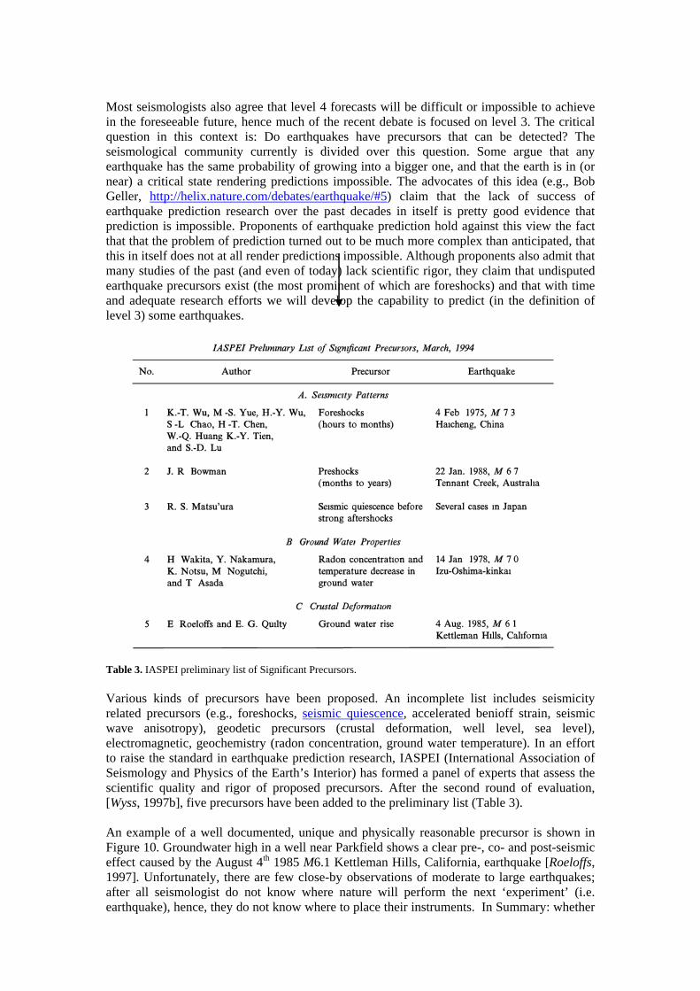
Table 3. IASPEI preliminary list of Significant Precursors. Various kinds of precursors have been proposed. An incomplete list includes seismicity related precursors (e.g., foreshocks, seismic quiescence, accelerated benioff strain, seismic wave anisotropy), geodetic precursors (crustal deformation, well level, sea level), electromagnetic, geochemistry (radon concentration, ground water temperature). In an effort to raise the standard in earthquake prediction research, IASPEI (International Association of Seismology and Physics of the Earth’s Interior) has formed a panel of experts that assess the scientific quality and rigor of proposed precursors. After the second round of evaluation, [Wyss, 1997b], five precursors have been added to the preliminary list (Table 3). An example of a well documented, unique and physically reasonable precursor is shown in Figure 10. Groundwater high in a well near Parkfield shows a clear pre-, co- and post-seismic effect caused by the August 4th 1985 M6.1 Kettleman Hills, California, earthquake [Roeloffs, 1997]. Unfortunately, there are few close-by observations of moderate to large earthquakes; after all seismologist do not know where nature will perform the next ‘experiment’ (i.e. earthquake), hence, they do not know where to place their instruments. In Summary: whether

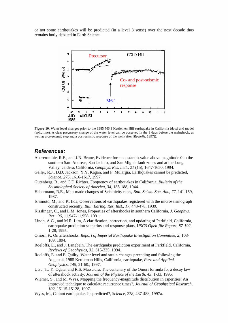
or not some earthquakes will be predicted (in a level 3 sense) over the next decade thus remains hotly debated in Earth Science.

Precursor

Co- and post-seismic response

M6.1

Figure 10. Water level changes prior to the 1985 M6.1 Kettlemen Hill earthquake in California (dots) and model (solid line). A clear precursory change of the water level can be observed in the 3 days before the mainshock, as well as a co-seismic step and a post-seismic response of the well (after [Roeloffs, 1997]).

References: Abercrombie, R.E., and J.N. Brune, Evidence for a constant b-value above magnitude 0 in the

southern San Andreas, San Jacinto, and San Miguel fault zones and at the Long Valley caldera, California, Geophys. Res. Lett., 21 (15), 1647-1650, 1994.

Geller, R.J., D.D. Jackson, Y.Y. Kagan, and F. Mulargia, Earthquakes cannot be predicted, Science, 275, 1616-1617, 1997.

Gutenberg, R., and C.F. Richter, Frequency of earthquakes in California, Bulletin of the Seismological Society of America, 34, 185-188, 1944.

Habermann, R.E., Man-made changes of Seismicity rates, Bull. Seism. Soc. Am., 77, 141-159, 1987.

Ishimoto, M., and K. Iida, Observations of earthquakes registered with the microseismograph constructed recently, Bull. Earthq. Res. Inst., 17, 443-478, 1939.

Kisslinger, C., and L.M. Jones, Properties of aftershocks in southern California, J. Geophys. Res., 96, 11,947-11,958, 1991.

Lindh, A.G., and M.R. Lim, A clarification, correction, and updating of Parkfield, California, earthquake prediction scenarios and response plans, USGS Open-file Report, 87-192, 1-28, 1995.

Omori, F., On aftershocks, Report of Imperial Earthquake Investigation Committee, 2, 103-109, 1894.

Roeloffs, E., and J. Langbein, The earthquake prediction experiment at Parkfield, California, Reviews of Geophysics, 32, 315-335, 1994.

Roeloffs, E. and E. Quilty, Water level and strain changes preceding and following the August 4, 1985 Kettleman Hills, California, earthquake, Pure and Applied Geophysics, 149, 21-60., 1997.

Utsu, T., Y. Ogata, and R.S. Matsu'ura, The centenary of the Omori formula for a decay law of aftershock activity, Journal of the Physics of the Earth, 43, 1-33, 1995.

Wiemer, S., and M. Wyss, Mapping the frequency-magnitude distribution in asperities: An improved technique to calculate recurrence times?, Journal of Geophysical Research, 102, 15115-15128, 1997.

Wyss, M., Cannot earthquakes be predicted?, Science, 278, 487-488, 1997a.

Wyss, M., Second round of evaluations of proposed earthquake precursors, Pure and Applied Geophysics, 149, 3-16, 1997b.

Zuniga, F.R., and S. Wiemer, Seismicity patterns: are they always related to natural causes?, Pure and Applied Geophysics, 155, 713-726, 1999.

Zuniga, R., and M. Wyss, Inadvertent changes in magnitude reported in earthquake catalogs: Influence on b-value estimates, Bulletin of the Seismological Society of America, 85, 1858-1866, 1995.

Appendix: Useful links for seismologists Glossary of seismological terms: http://wwwneic.cr.usgs.gov/neis/general/handouts/glossary.html Seismo-surfing the Internet (most comprehensive list of seismological institutes). http://www.geophys.washington.edu/seismosurfing.html Information about earthquakes in Switzerland: http://www.seismo.ethz.ch/ US. Geological Service; National Earthquake Information Center (includes near real-time list of recent worldwide earthquakes): http://wwwneic.cr.usgs.gov/ Southern California Earthquake Data Center: Education Modules http://www.scecdc.scec.org/Module/module.html Virtual Earthquake: Locate an event on the Internet http://vcourseware.sonoma.edu/VirtualEarthquake/VQuakeExecute.html Earthquake legends: http://www.fema.gov/kids/eqlegnd.htm Observatories and Research Facilities for European Seismology (includes seismological software archive): http://orfeus.knmi.nl/ How to prepare for the next big earthquake http://www.uaf.edu/seagrant/earthquake/