Wide/Narrow Band Spectrograms• Wide band (left)

– Combines harmonics– Voiced speech vocal fold

pulses (glottis air puffs) show as vertical lines

• Narrow band(right) – Individual harmonics– Narrow-band displays

formants horizontally– No vocal pulses shown

• Display parameters– Generally log power

(log(amplitude2)– Frame shift: 1 ms typical

Spectrogram for a vowel sound

Spectrograms: vowel with varying pitch

Frame Positioning • Pitch-synchronous

– Centered around a pitch period– Varied size frames– Unvoiced sections assume fixed pitch period– Challenge: Determine exact pitch period locations

• Pitch-asynchronous– Fixed frames and shifts

• typically 25-30 ms frame width with a 10 ms frame shift

• Tradeoffs– Too large: contains more than one phoneme– Too small: cannot determine F0 or the harmonics

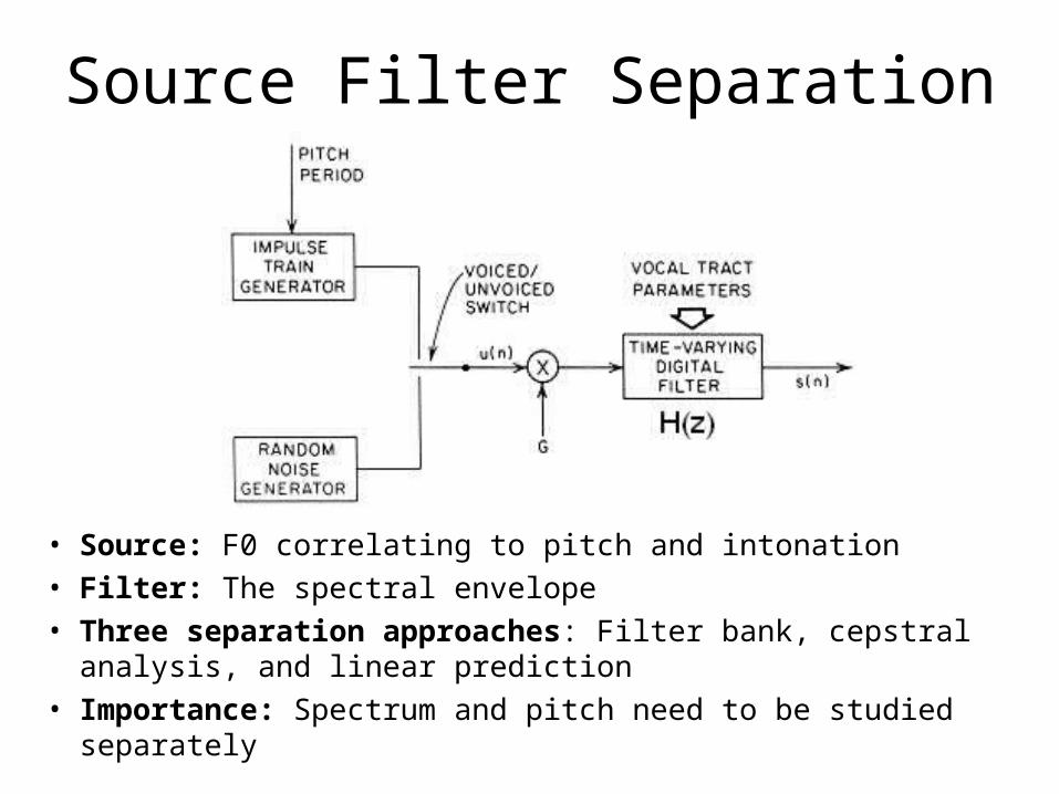
Source Filter Separation

• Source: F0 correlating to pitch and intonation• Filter: The spectral envelope• Three separation approaches: Filter bank, cepstral analysis,

and linear prediction• Importance: Spectrum and pitch need to be studied separately

Filter Bank• Time Domain

– Series of linear band pass filters

• Frequency Domain– Window a frame (Ex: Hamming)– Perform Fourier Transform– Warp frequencies (Ex: Mel scale)– Compute weighted sum of each bin

• Advantage– simple and robust for finding spectral envelope– Okay for ASR (unless language is tonal)

• Disadvantage– Lose too much detail to find pitch. – Peaks can fall between harmonics; not good for TTS

The Cepstrum• Definition: c[n] = F -1{log(|F(x[n]|}

• Note: Sometimes the Cepstrum is taken on the square of the spectrum rather than on the log of the spectrum

• Treat the spectrum as a wave– Formant frequency is slow– Glottal pulses are fast– Cepstrum separates the two

• Cepstral Terminology – Cepstrum is Spectrum in reverse– Quefrency instead of frequency– Lifter instead of filter

Separating Source from Vocal Filter• Source

– Excites particular fundamental frequencies– The glottis source sometimes is noisy

• Filter– The source is filtered resulting in vocal tract resonances

• Goal: Separate excitation frequencies from the filter• Process

1. Time domain convolves source with filter (u[n] * v[n])2. Convolution multiplies in the frequency domain (UV)3. Log converts multiplication to a sum (log(UV) = log(U) + log(V))4. The V (filter) varies slowly; the U (excitation) varies quickly.5. The inverse operation separates u[n] and v[n] into different

quefrencies• Observations

– There are no pitch excitations in unvoiced speech– Cepstral analysis works well for speech recognition applications

Cepstrum Process IllustrationTime

Speech Signal

Frequency

Log Frequency

Time

Cepstrums of Excitation

After FFT

After log(FFT)

After inverse FFT of log

Spectral envelope on the left, F0 is one of the excitations

Cepstrum Samples

Note: Band passing frequencies below 100 or greater than 900 can help

Cepstral Mean Normalization (CMN)

• For each window we perform a Cepstral analysis• Mel scaled Quefrencies summed into 13 to 39 bins

• Each bin represents a Cepstral vector X = {x0, x1, …, xT-1}

• Compute the mean of each vector coefficientµk = 1/T ∑t=0,T-1xt where k is a vector coefficient

• Subtract uk from coefficient k of each vector X

For Automatic Speech Recognition

Cepstral Evaluation

• The Cepstral process eliminates phase data. However, human perception largely, but not totally, ignores phase

• Use the lower quefrencies to study the vocal filter• Use the peak to study pitch and glottis behavior• Zeroing the pitch portion of the Cepstrum and

transforming back to the frequency domain is an approach for speech recognition

• Disadvantage of Cepstrals: They are difficult to interpret using a visual plot

Time Domain Pitch Detection• Recall the autocorrelation pitch

detection algorithm– Correlate a window of speech

with a previous window– Find the best match– Problem: too many false peaks

• Peak and center clipping– Algorithm to reduce false peaks– clip the top/bottom of a signal– Center the remainder around 0

• Other alternatives– Researchers propose many other

pitch detection algorithms – There are much debate as to

which is the best

Epoch Detection• Simply determining the pitch is not sufficient for

synthesis– Unit selection requires accurate anchors to be able to

merge segments of speech – Otherwise clicks and other artifacts will be heard

• Pitch-marking or epoch-detection attempt to accurately mark pitch points– Mark peaks or troughs– Mark Instant of glottal closure (large negative pulse)

• There are many algorithms proposed, but this remains an open research area

Linear Prediction Coding (LPC)

• Originally developed to compress (code) speech• Although coding pertains to compression, the term

LPC has much broader implications in NLP– LPC is equivalent to the vocal tract model (Week 6)– LPC is another computational method to

• Compute vocal tract reflection coefficients• Compute vocal tract filter coefficients

– LPC is useful to separating source (glottis) from filter (vocal tract)

Linear Predictive Encoding (LPC)

Concept

• Guess at the next value using a set of previous values

• Instead of outputting the actual data, output the error from the guess

• Less bits should be needed if the guess is good

Pseudo Code

WHILE not EOF READ sample n (s[n])

x = prediction() error = x – s[n] IF error too large to fit in compressed size WRITE special code WRITE s[n] ELSE WRITE error

One approach: There are many others with better compression

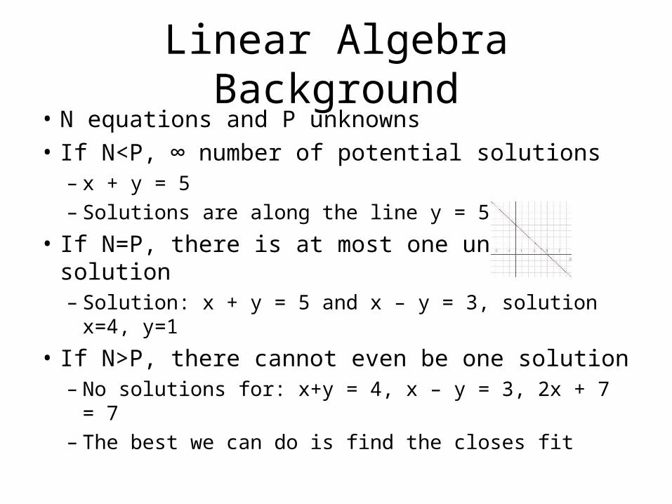
Linear Algebra Background• N equations and P unknowns• If N<P, ∞ number of potential solutions

– x + y = 5– Solutions are along the line y = 5-x

• If N=P, there is at most one unique solution– Solution: x + y = 5 and x – y = 3, solution x=4, y=1

• If N>P, there cannot even be one solution– No solutions for: x+y = 4, x – y = 3, 2x + 7 = 7– The best we can do is find the closes fit

Least Squares: minimize error

• First Approach: Linear algebra – find orthogonal projections of vectors onto the best fit

• Second Approach: Calculus – Use derivative with zero slope to find best fit

Solving n equations and n unknowns

• Gaussian Elimination – Complexity: O(n3)

• Successive Iteration– Complexity varies

• Cholskey Decomposition– More efficient, still O(n3)

• Levenson-Durbin– Complexity: O(n2)– Works for symmetric

Toplitz matrices

Definitions for any matrix, ATranspose (AT): Replace aij by aji for all i and jSymmetric: AT = APositive Definite: No complex solutions Toplitz: Diagonals to the right all have equal valuesLower/Upper triangular: No non zero values above/below diagonal

Symmetric Toeplitz Matrices

• Flipping rows and columns produces the same matrix• Every diagonal to the right contains the same value

Example

Levinson Durbin Algorithm

Verify results by plugging a41, a42, a43, a44 back into the equations

6/5(1) + 0(2) + (0)3 + 1/5(4) = 2, 6/5(2) + 0(1) + 0(2) + 1/5(3) = 36/5(3) + 0(2) + 0(1) + 1/5(2) = 4, 6/5(4) + 0(3) + 0(2) + 1/5(1) = 5

Step 0 E0 = 1 [r0 Initial Value]

Step 1 E1 = -3 [ (1-k12)E0] k1 = 2 [r1/E0]

Step 2 E2 = -8/3 [ (1-k22)E1] k2 = 1/3 [(r2 – a11r1)/E1]

Step 3 E3 = -5/2 [(1-k32)E2 k3 = 1/4 [(r3 – a21r2 – a22r1)/E2]

Step 4 E4 = -12/5 [(1-k42) E3] k4 = 1/5 [r4 – a31r3 – a32r2 – a33r1)/E3]

a11=2 [k1]

a21=4/3 [a11-k2a11] a22=1/3[k2]

a31=5/4 [a21-k3a22] a32=0 [a22-k3a21] a33=1/4 [k3]

a41=6/5 [a31-k4a33] a42=0 [a32-k4a32] a43=0[a33-k4a31] a44=1/5[k4]

or

Levinson-Durbin Pseudo Code

E0 = r0

FOR step = 1 TO Pkstep = ri

FOR i = 1 TO step-1 THEN kstep -= ai-1,i * rstep-i

kstep /= Estep-1

Estep = (1 – k2step)Estep-1

astep,step = kstep-1

For i = 1 TO step-1 THEN astep,i = astep-1,I – kstep*astep-1, step-i

Note: ri are the row 1 matrix coefficients

Cholesky Decomposition• Requirements:

– Symmetric (same matrix if flip rows and columns)– Positive definite matrix (no complex solutions)

• Solution– Factor matrix A into: A = LLT where L is lower triangular– Perform forward substitution to solve: L(LT[ak]) = [bk]

– Use the resulting vector, [xi], in the above step to perform a backward substitution to solve for LT[ak] = [xi]

• Complexity– Factoring step O(n3/3) – Forward substitution: n2

– Backward substitution: n2

Cholesky Factorization

Result:

Cholesky Factorization Pseudo Code

• Column index: k• Row index: j• Elements of matrix A: aij

• Elements of matrix L: l

FOR k=1 TO n-1 lkk = a½

kk

FOR j = k+1 TO n ljk = ajk/ lkk

FOR j = k+1 TO nFOR i = j TO n aij = aij – lik ljk

lnn = ann

{1, 2, 3, 4, 5, 6, 7, 8, 9, 10, 11, 12, 13, 14, 15, 16}

Illustration: Linear Prediction

Goal: Estimate yn using the three previous valuesyn ≈ a1 yn-1 + a2 yn-2 + a3 yn-3

Three ak coefficients, Frame size of 16Thirteen equations and three unknowns

Note: The equation is an IIR filter

LPC Basics• Predict x[n] from x[n-1], … , x[n-P]

– en = yn - ∑k=1,P ak yn-k

– en is the error between the projection and the actual value

– The goal is to find the coefficients that produce the smallest en value

• Concept– Square the error– take the partial derivative with respect to each ak

– Find the solution with zero derivative (the minimum).

• Result : P equations with P unknowns

Finding the Best LPC Estimate• One linear prediction equation: en = yn - ∑k=1,P ak yn-k

– Over a whole frame we have n equations and k unknowns• Sum en over the entire frame: E = ∑n=0,N-1(yn - ∑k=1,P ak yn-k)

• Square the total error: E2 = ∑n=0,N-1 (yn - ∑k=1,P ak yn-k)2

• Take partial derivative with respect to each a j; generates P equations (Ej)

– Like a regular derivative treating only a j as a variable2Ej = 2(∑n=0,N-1 (yn - ∑k=1,P akyn-k)yn-j)

– Calculus Chain Rule: if y = y(u(x)) then dy/dx = dy/du * du/dx• Set each Ej to zero (zero derivative) to find the minimum P errors

for j = 1 to P then 0 = ∑n=0,N-1 (yn - ∑k=1,P akyn-k)yn-j (j indicates the equation)

• Rearrange terms: for each j of the P equations, ∑n=0,N-1 ynyn-j=∑n=0,N-1∑k=1,Pakyn-kyn-j=∑k=1,P∑n=1,Nakyn-kyn-j =∑k=1,Pakφ(j,k)=φ(j,0)

• Result: P equations and P unknowns where φ(j,k) = ∑n=0,N-1 yn-kyn-j

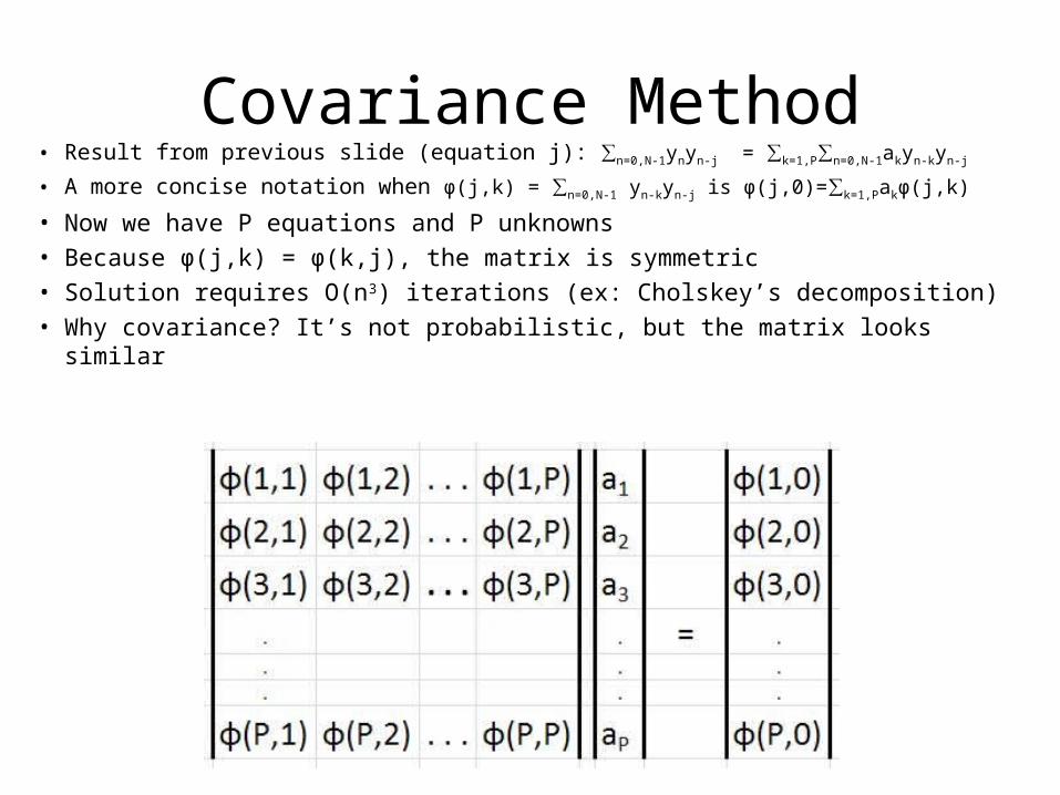
Covariance Method• Result from previous slide (equation j): ∑n=0,N-1ynyn-j = ∑k=1,P∑n=0,N-1akyn-kyn-j

• A more concise notation when φ(j,k) = ∑n=0,N-1 yn-kyn-j is φ(j,0)=∑k=1,Pakφ(j,k)

• Now we have P equations and P unknowns• Because φ(j,k) = φ(k,j), the matrix is symmetric• Solution requires O(n3) iterations (ex: Cholskey’s decomposition)• Why covariance? It’s not probabilistic, but the matrix looks similar

Covariance Example

• Signal: {…, 3, 2, -1, -3, -5, -2, 0, 1, 2, 4, 3, 1, 0, -1, -2, -4, -1, 0, 3, 1, 0, …}• Frame: {-5, -2, 0, 1, 2, 4, 3, 1}, Number of coefficients: 3• φ(1,1) = -3*-3 +-5*-5 + -2*-2 + 0*0 + 1*1 + 2*2 + 4*4 + 3*3 = 68 • φ(2,1) = -1*-3 +-3*-5 + -5*-2 + -2*0 + 0*1 + 1*2 + 2*4 + 4*3 = 50 • φ(3,1) = 2*-3 +-1*-5 + -3*-2 + -5*0 + -2*1 + 0*2 + 1*4 + 2*3 = 13 • φ(1,2) = -3*-1 +-5*-3 + -2*-5 + 0*-2 + 1*0 + 2*1 + 4*2 + 3*4 = 50 • φ(2,2) = -1*-1 +-3*-3 + -5*-5 + -2*-2 + 0*0 + 1*1 + 2*2 + 4*4 = 60 • φ(3,2) = 2*-1 +-1*-3 + -3*-5 + -5*-2 + -2*0 + 0*1 + 1*2 + 2*4 = 36 • φ(1,3) = -3*2 +-5*-1 + -2*-3 + 0*-5 + 1*-2 + 2*0 + 4*1 + 3*2 = 13 • φ(2,3) = -1*2 +-3*-1 + -5*-3 + -2*-5 + 0*-2 + 1*0 + 2*1 + 4*2 = 36 • φ(3,3) = 2*2 +-1*-1 + -3*-3 + -5*-5 + -2*-2 + 0*0 + 1*1 + 2*2 = 48 • φ(1,0) = -3*-5 +-5*-2 + -2*0 + 0*1 + 1*2 + 2*4 + 4*3 + 3*1 = 50 • φ(2,0) = -1*-5 +-3*-2 + -5*0 + -2*1 + 0*2 + 1*4 + 2*3 + 4*1 = 23 • φ(3,0) = 2*-5 +-1*-2 + -3*0 + -5*1 + -2*2 + 0*4 + 1*3 + 2*1 = -12

Recall: φ(j,k) = ∑n=start,start+N-1 yn-kyn-j Where equation j is: φ(j,0) = ∑k=1,Pakφ(j,k)

Auto-Correlation Method• Assume: all values of the signal outside of 0<j<N-1 is zero

• Correlate from -∞ to ∞ (most values are 0)• The LPC formula for φ becomes: φ(j,k)=∑n=0,N-1-(j-k) ynyn+(j-k)=R(j-k)

• The Matrix is now in the Toplitz format– The Levinson Durbin algorithm applies – Implementation complexity: O(n2)

Auto Correlation Example

• Signal: {…, 3, 2, -1, -3, -5, -2, 0, 1, 2, 4, 3, 1, 0, -1, -2, -4, -1, 0, 3, 1, 0, …}• Frame: {-5, -2, 0, 1, 2, 4, 3, 1}, Number of coefficients: 3

• R(0) = -5*-5 + -2*-2 + 0*0 + 1*1 + 2*2 + 4*4 + 3*3 + 1*1 = 60• R(1) = -5*-2 + -2*0 + 0*1 + 1*2 + 2*4 + 4*3 + 3*1 = 35• R(2) = -5*0 + -2*1 + 0*2 + 1*4 + 2*3 + 4*1 = 12• R(3) = -5*1 + -2*2 + 0*4 + 1*3 + 2*1 = -4

Recall: φ(j,k)=∑n=0,N-1-(j-k) ynyn+(j-k)=R(j-k)Where equation j is: R(j) = ∑k=1,P R(j-k)ak

Notation: j is the row, k is the column

LPC Transfer Function• Predict the values of the next sample

Ŝ[n] = ∑ k=1,p ak s[n−k]

• The error signal (e[n]), is the LPC residuale[n]=s[n]− ŝ[n] = s[n]− ∑ k=1,p ak s[n−k]

• Perform a Z-transform of both sidesE(z)=S(z)− ∑k=1,pak S(z)z−k

• Factor S(z)E(z) = S(z)[ 1−∑k=1,p ak z−k ]=S(z)A(z)

• Compute the transfer function: S(z) = E(z)/A(z)

• Conclusion: LPC provides us with an all pole filter

LPC Coding and Synthesis Models

Synthesis Model

Coding Model

ConclusionThe LPC all-pole model can code and synthesizes speech

The LPC Model• The LPC estimate

– An all-pole IR filter: yn = Gxn - ∑k=1,N ak yn – The Gxn residual attempts to model the glottal source– LPC estimates the separation of source from filter

• Challenges (Problems in synthesis)– The residual does not accurately model the source (glottis) – The filter does not model radiation from the lips– The model does not account for nasal resonances

• Possible solutions– Additional poles can increase the accuracy to a point

• 1 pole pair for each 1k of sampling rate• 2 more pairs can better estimate the source and lips

– Introduce zeroes into the model– More robust analysis of the glottal source and lip radiation

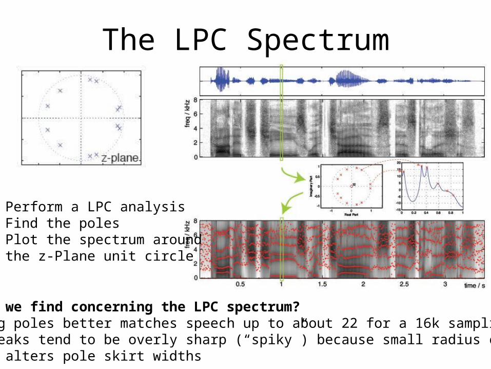
The LPC Spectrum

1. Perform a LPC analysis2. Find the poles3. Plot the spectrum around

the z-Plane unit circle

What do we find concerning the LPC spectrum?1.Adding poles better matches speech up to about 22 for a 16k sampling rate2.The peaks tend to be overly sharp (“spiky”) because small radius changesgreatly alters pole skirt widths

PARCOR• Definition: [PAR]tial auto [COR]relation coefficients

– LPC coefficients are: a1, a2, … aP

– PARCOR coefficients are: k1, k2, … kP

– It is easy to compute PARCOR from LPC and visa versa

• Review– Rectangular tubes have reflection coefficients

rk = (Ak+1 – Ak)/(Ak+1 + Ak)

– With algebra the ratio of areas between tubes are:Ak/Ak+1 = (1-rk)/(1+rk)

• Importance– LPC is equivalent to the tube model of the vocal tract– Log[Ak+1/Ak] = log[(1-ki)/(1+ki)]

– We can adjust the LPC parameters based on PARCOR

Relationship to Tube Model

Given PARCOR, compute LPC

FOR i = 1 TO Pxi,i = ki

if (i>1) then FOR j = 1 TO i-1xi,j = xi-1,j – kixi-1,i-j

FOR j=1 TO P THEN aj = xP,j

Given LPC, compute PARCORFOR j = 1 TO P THEN xP,j = aj

kp = xP,P

FOR i = P TO 2 STEP -1FOR j = 1 TO i-1

xi-1,j = (xi,j + kixi,i-j)/(1-ki2)

ki-1 = xi-1,i-1

Notes: ki are PARCOR coefficientsai are LPC coefficientsxi,j is a temporary work array

Line Spectrum Pairs• Overview

– Filter with an additional coefficient– Uses the equations on the right– The New filter models:

• A completely closed glottis• Completely open lips

• Characteristics– Spectrum shown as lines because of infinite amplitudes of formants– Forces zeros and poles to be interspersed on the unit circle

• Advantages – Easier to estimate formants– Less sensitive to quantization errors

LPC and the Source Signal• Experiments show

– Glottis requires both zeros and poles– It requires less poles than the vocal function– LPC combines the glottal and vocal tract poles

• If U(z) = I(z)G(z)– U(z) = source function– I(z) = Impulse sequence– G(z) Glottal filter

• Transfer function

• Goal: separate glottal poles from the LPC predictor

∏k=0,Mbkz-k

U(Z) = I (z)1 - ∏j=0,Lajz-j

Closed Phase Analysis

• Find Instant of glottal closure – Epoch detection algorithm

• Divide signal– closed phase (glottis does not affect LPC predictors)– open phases (glottis has significant impact)

• Strategy– Compute the G filter over a number of pitch periods– Perform an inverse filter to obtain the glottal signal

Open Phase Analysis • Problem: It is not easy to find the instance of glottal closure • Goal: add extra poles to the model• Advantages

– Human hearing is more sensitive to peaks than to valleys– The tube model and LPC are all-pole systems

• Disadvantages: – Relationships between the poles and the formants becomes obscure– Extra poles can approximate a zero, but not perfectly

• How can extra poles approximate zeros– For example if x,y ≠ -1, then consider the following derivation

1-x = 1/(1+y)1 = (1-x)(1+y) = 1 +y –x –xy = 1 + y(1-x) – xTherefore: y = x/(1-x)