Why retailers cluster: An agent model of location choice onsupply chains

A THESISSUBMITTED TO THE FACULTY OF THE GRADUATE SCHOOL

OF THE UNIVERSITY OF MINNESOTABY

Arthur Yan Huang

IN PARTIAL FULFILLMENT OF THE REQUIREMENTSFOR THE DEGREE OFMASTER OF SCIENCE

David M. Levinson, Adviser

March 2010

c© Arthur Yan Huang 2010ALL RIGHTS RESERVED

ABSTRACT

This research investigates the emergence of retail clusters on supply chains comprised of

suppliers, retailers, and consumers. An agent-based model is employed to study retail lo-

cation choice in a market of homogeneous goods and a market of complementary goods.

On a circle comprised of discrete locales, retailers play a non-cooperative game by choos-

ing locales to maximize profits which are impacted by their distance to consumers and to

suppliers. The findings disclose that in a market of homogeneous products symmetric distri-

butions of retail clusters rise out of competition between individual retailers; average cluster

density and cluster size change dynamically as retailers enter the market. In a market of

two complementary goods, multiple equilibria of retail distributions are found to be com-

mon; a single cluster of retailers has the highest probability to emerge. Overall, my results

demonstrate that retail clusters emerge from the balance between retailers’ proximity to

their customers, their competitors, their complements, and their suppliers.

i

Acknowledgement

My interest in complex systems emerged in 2006 when I attended the Santa Fe Institute

Complex Systems Summer School. Before I attended the summer school, I was puzzled

about what I should do in research. While having degrees in automatic and computer en-

gineering, I felt that I think more like a social scientist. The problems in the world are

complex, and maximizing or minimizing certain narrowly-defined objectives from the engi-

neering point of view—while may be beautiful in mathematical terms—does not often seem

to provide reasonable and acceptable solutions for the society. Yet in this summer school,

I was amazed by how people from a variety of academic backgrounds (such as sociology,

biology, and engineering) can work together to examine systems from a holistic perspective

that would not have been otherwise possible. Also during this period of time, I, along with

other graduate students worldwide, finished a project of analyzing the topology of Chinese

airline networks. I sensed that there was more work to do to better our transportation

systems and city life from a new perspective. After the summer school, I further read some

books on complex systems and network theory, including Roger Lewin’s Complexity: Life

at the Edge of Chaos, and Duncan Watts’s Small Worlds. I was completely drawn to the

world of complexity.

When I started to search for Ph.D. programs, I focused on interdisciplinary programs on

complex systems, transportation, urban policy, and urbanization. I found that Prof. David

Levinson has done lots of work in this field, and therefore I applied to his program. I was

lucky to be admitted, so here I am. One may wonder why a seemingly inconsequential event

(such as attending a summer school) can have such an important and irreversible influence

on one’s career. My past experience perfectly attests to the theory of path dependence.

The greatest impact on my research and my working style comes from my advisor

Prof. David Levinson, who gives me the freedom to work on the topics I am interested in.

Moreover, we’ve had lots of discussions on research not just in weekly meetings but also

in daily emails. I am very appreciative of his support. In particular, I am grateful for his

patience and open-mindedness for my sometimes unusual ideas and curiosity.

In the past two years I spent most of my time in Office 275 of the Nexus research group.

This is a fun group of people to work with. Many interesting discussions or debates are

ii

happening here every day, not just on research, but also on other parts of life. While we do

not always agree with each other, I have learned a lot from each of them.

Many thanks go to my friends at the University and at my church, whose love, encour-

agement, and care have enormously strengthened me in almost every aspect of my life. I

am blessed to have them around. Also, I want to thank my dear mom and dad who always

tell me to finish what I have started. This work is as much theirs as it is mine.

iii

Contents

List of Tables vi

List of Figures vii

1 Introduction 1

2 Problem statement and literature review 3

2.1 Motivation and Problem Statement . . . . . . . . . . . . . . . . . . . . . . . 3

2.2 Literature on business location choice . . . . . . . . . . . . . . . . . . . . . 4

2.3 Retail geography . . . . . . . . . . . . . . . . . . . . . . . . . . . . . . . . . 5

2.4 Previous urban simulation models . . . . . . . . . . . . . . . . . . . . . . . 6

2.5 Agent-based modeling in transportation and land use . . . . . . . . . . . . . 6

3 The agent-based model 8

3.1 Model structure . . . . . . . . . . . . . . . . . . . . . . . . . . . . . . . . . . 8

3.2 Assumptions and definition of cluster . . . . . . . . . . . . . . . . . . . . . . 9

3.3 Consumers . . . . . . . . . . . . . . . . . . . . . . . . . . . . . . . . . . . . 11

3.4 Retailers . . . . . . . . . . . . . . . . . . . . . . . . . . . . . . . . . . . . . . 13

3.5 Suppliers . . . . . . . . . . . . . . . . . . . . . . . . . . . . . . . . . . . . . 14

4 Results and analysis 15

4.1 The market of homogeneous goods . . . . . . . . . . . . . . . . . . . . . . . 15

4.1.1 Base case . . . . . . . . . . . . . . . . . . . . . . . . . . . . . . . . . 15

4.1.2 Heterogeneous population . . . . . . . . . . . . . . . . . . . . . . . . 18

4.1.3 Sensitivity tests . . . . . . . . . . . . . . . . . . . . . . . . . . . . . . 19

4.2 The market of complementary goods . . . . . . . . . . . . . . . . . . . . . . 23

iv

4.2.1 Base case . . . . . . . . . . . . . . . . . . . . . . . . . . . . . . . . . 23

4.2.2 Sensitivity tests . . . . . . . . . . . . . . . . . . . . . . . . . . . . . . 25

5 Discussion and conclusions 29

5.1 Discussion . . . . . . . . . . . . . . . . . . . . . . . . . . . . . . . . . . . . . 29

5.2 Conclusion . . . . . . . . . . . . . . . . . . . . . . . . . . . . . . . . . . . . 30

Bibliography 32

v

List of Tables

3.1 List of parameters used in the models . . . . . . . . . . . . . . . . . . . . . . . . . 10

4.1 Values of parameters (Model 1: homogeneous goods; Model 2: complementary goods) . . 16

vi

List of Figures

3.1 Model structure . . . . . . . . . . . . . . . . . . . . . . . . . . . . . . . . . . . 9

3.2 Exemplary retail distribution patterns on a circle of discrete locales. Fig. 3.2-1 has five

clusters, each of which has only one retailer; therefore average cluster density equals 1.

Fig. 3.2-2 has three clusters, one cluster has two adjacent retailers; one cluster has only

one retailer; the rest one has two co-locating retailers. The average cluster density equals

(2+1+1)/3 = 1.33. Fig. 3.2-3 has two clusters; one cluster has only one retailer, while

the other has four retailers covering three locales. The average cluster density equals

(1+4/3)/2=1.17. . . . . . . . . . . . . . . . . . . . . . . . . . . . . . . . . . . . 12

4.1 Number of clusters and average cluster density. Fig.4.1-1: Number of clusters emerged

as the number of retailers increases from 2 to 100; Fig.4.1-2: Average cluster density as

retailers rises from 2 to 100. . . . . . . . . . . . . . . . . . . . . . . . . . . . . . 16

4.2 Examples of retail distribution patterns for different numbers of retailers in a market of

homogeneous goods (plotted in Pajek (Batagelj and Mrvar, 2009)). (Red circles stand for

retailers, and gray diamonds represent suppliers. Objects sitting on top of each other mean

that they share the same locale; adjacent objects indicate that they are geographically

adjacent.). Fig.4.2-1 displays the distribution pattern of 5 retailers. Fig.4.2-2 shows the

pattern of 10 retailers. Fig.4.2-3, Fig.4.2-4, Fig.4.2-5, and Fig.4.2-6 respectively exhibit

retail spatial patterns for 20, 30, 60, and 100 retailers. . . . . . . . . . . . . . . . . . 17

4.3 Demand in different locations, with individuals’ demand following normal distribution

(mean value equals 20 and st. dev. equals 10). . . . . . . . . . . . . . . . . . . . . 18

4.4 Retail distribution pattern in equilibrium, with individuals’ demand following normal dis-

tribution. . . . . . . . . . . . . . . . . . . . . . . . . . . . . . . . . . . . . . . 19

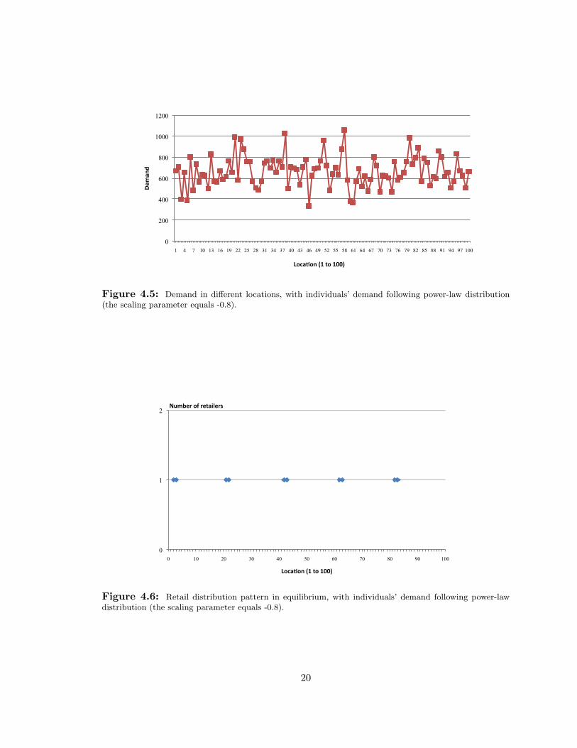
4.5 Demand in different locations, with individuals’ demand following power-law distribution

(the scaling parameter equals -0.8). . . . . . . . . . . . . . . . . . . . . . . . . . . 20

vii

4.6 Retail distribution pattern in equilibrium, with individuals’ demand following power-law

distribution (the scaling parameter equals -0.8). . . . . . . . . . . . . . . . . . . . . 20

4.7 Average cluster densities for the scenarios with retailers ranging from 2 to 30: results of

sensitivity tests on β (scaling parameter). . . . . . . . . . . . . . . . . . . . . . . 21

4.8 Average cluster densities for the scenarios with retailers ranging from 2 to 30: results of

sensitivity test on u (unit shipping cost). . . . . . . . . . . . . . . . . . . . . . . . 22

4.9 Individual consumer demand on product x increases with the rising of the number of re-

tailers, yet does not exceed 60. When the number of retailers exceeds 26, average consumer

demand reaches 60 (the upper limit of individual consumer demand) and stays constant

thereafter. . . . . . . . . . . . . . . . . . . . . . . . . . . . . . . . . . . . . . . 24

4.10 A comparison of retail average profit with and without consumer demand elasticity for the

number of retailers from 2 to 100. The curve of retail average profit without demand elas-

ticity (base case) goes under the curve with demand elasticity; the profit gap is particularly

salient when the number of retailers is between 5 and 40. . . . . . . . . . . . . . . . 24

4.11 Probability distribution of the numbers of clusters with retailers ranging from 4 to 40

(where the number of retailers of x equals the number of retailers of y), with total 20

suppliers (10 suppliers of x and 10 suppliers of y). The case of one cluster has the highest

probability to appear of all the cases. . . . . . . . . . . . . . . . . . . . . . . . . 26

4.12 Probability distribution of the numbers of clusters with 10 retailers of product x and the

number of retailers of product y ranging from 2 to 16 (shown in the horizontal axis). The

case of only one cluster has the highest likelihood to emerge. The greater gap between the

number of retailers of product x and the number of retailers of product y, the more likely

that the case of fewer clusters will emerge. . . . . . . . . . . . . . . . . . . . . . . 27

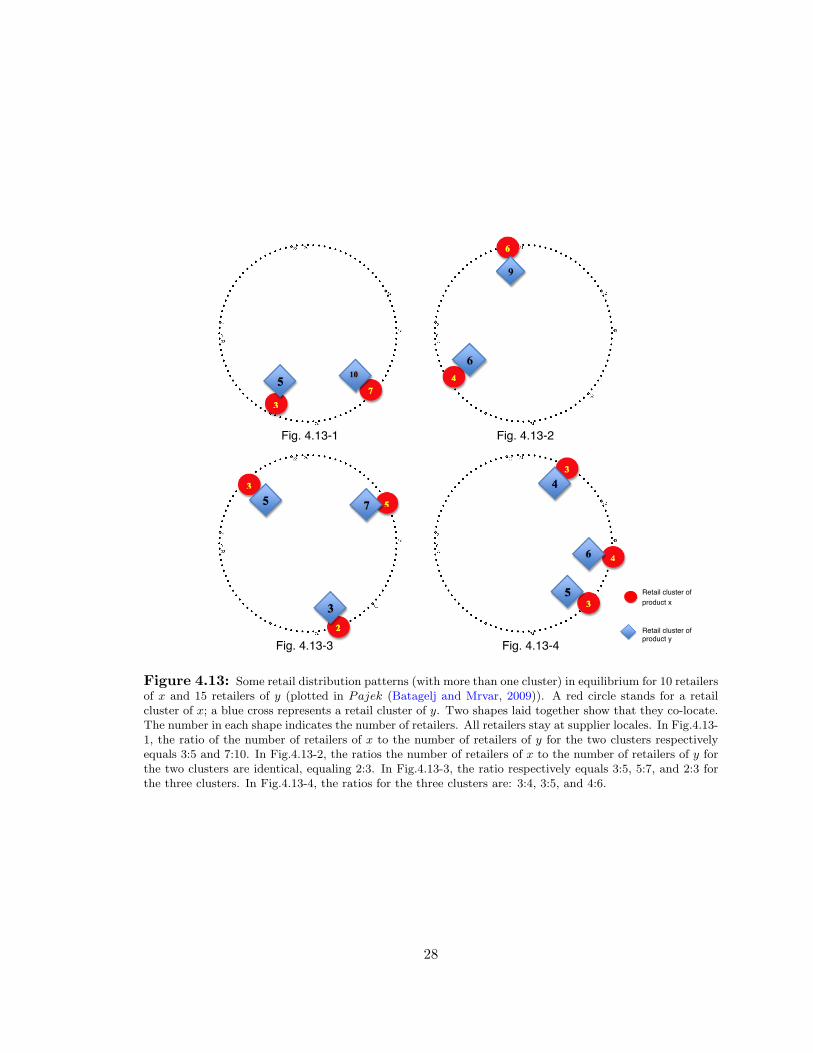
4.13 Some retail distribution patterns (with more than one cluster) in equilibrium for 10 retailers

of x and 15 retailers of y (plotted in Pajek (Batagelj and Mrvar, 2009)). A red circle stands

for a retail cluster of x; a blue cross represents a retail cluster of y. Two shapes laid together

show that they co-locate. The number in each shape indicates the number of retailers. All

retailers stay at supplier locales. In Fig.4.13-1, the ratio of the number of retailers of x

to the number of retailers of y for the two clusters respectively equals 3:5 and 7:10. In

Fig.4.13-2, the ratios the number of retailers of x to the number of retailers of y for the

two clusters are identical, equaling 2:3. In Fig.4.13-3, the ratio respectively equals 3:5, 5:7,

and 2:3 for the three clusters. In Fig.4.13-4, the ratios for the three clusters are: 3:4, 3:5,

and 4:6. . . . . . . . . . . . . . . . . . . . . . . . . . . . . . . . . . . . . . . 28

viii

Chapter 1

Introduction

The locations of human activities shape travel behavior and have consequent outcomes

on air pollution, noise, and safety, and overall social welfare. Hierarchical distributions of

economic activities and resources occur in almost every region and nation. Famous examples

are the US carpet production industry, disproportionately concentrated in Dalton, Georgia

(Krugman, 1991) and the Italian textile industry in Prato (Porter, 1990). Within cities,

there are different business clusters; to illustrate, Kappabashi, or Kitchen Town, in Tokyo

is a district of competing businesses supplying cookware. Friedmann (1986), in his seminal

work about the network of world cities, argued that inter-city relations lead to a complex

spatial hierarchy of world cities. Sassen (1991) identified New York, London and Tokyo as

leading examples of world cities and suggested that despite their different provenance, each

city had experienced the same economic processes and resultant social change.

Contemporary globalization, pushed by fast-developing communication technology and

decreasing transport cost, leads to two seemingly contradictory yet complementary spatial

phenomenon: agglomeration of economic activities and decentralization (Taylor, 2004). On

the one hand, we are impressed by the flourishing of the Silicon Valley as a major global

Information Technology R&D center. On the other hand, a large proportion of the large-

scale materials-intensive forms of manufacturing that formerly clustered near the core of

the metropolis has decentralized to suburban and peripheral areas (Scott, 1988). Two

questions naturally follow this: what can we learn from these phenomena? How should

planners and transportation engineers respond in such a context for the betterment of

1

social welfare? Policy makers are eager to know how to react in an economic system with

inherent clustering characteristics, how to respond to win “founder’s advantage” in global

competition, and how to behave if they are initially in a disadvantaged position. Properly

answering such questions is vital for policy makers to make the world a better place to live.

The world economy has become increasingly connected, and almost all business activities

worldwide can be seen as interlinked in terms of technology, capital, labor, demand, or

supply. When almost all business activities worldwide are interlinked in terms of technology,

capital, labor, demand, or supply, to disentangle the cause-and-effect relationship of daily

phenomenon poses a great challenge. It is even more so for economic geography studies

due to its complexity at both temporal and spatial dimensions. The lack of understanding

about the principles of the distribution of human economic activities often results in ill

policy-makings.

While acknowledging regional differences a priori, this research seeks to find an under-

lying mechanism that leads in some cases to spatial concentration of seemingly competitive

economic activities, and in others to their dispersal. By building simulation models, I hope

to better understand the “invisible hand” that directs the spatial distribution of business

activities.

The reminder of this thesis is organized as follows. Chapter 2 describes my motivation

for this research and the research questions. Also, I review the literature on business

location choice and the agent-based approach in examining transportation and land use

systems. Chapter 3 introduces the agent-based model of retail location choice on supply

chains. Chapter 4 displays and analyzes the simulation results. The last chapter discusses

the implications of the results and concludes the thesis.

2

Chapter 2

Problem statement and literature

review

2.1 Motivation and Problem Statement

Retail clusters are geographic concentrations of competing, complementary, and interde-

pendent stores. Rules governing the agglomeration and dispersion of retailers depend on

numerous factors that may impact retail distribution patterns and consumer preferences.

Traditional studies on retail geography and spatial clusters - while providing insights about

the factors influencing retail location choice - often neglect complex interactive behavior

among agents and heterogeneous population. From a systems perspective, urban areas are

not only concentrations of places and people, but also “systems of organized complexity”

where a large number of quantities vary simultaneously and “[interrelate] into an organic

whole” (Jacobs, 1961).

Adopting a similar view, this research attempts to understand what can promote the

concentration of human activities. This understanding suggests two insights I need to

consider in modeling this phenomenon: first, numerous supply chains are interwoven in

the urban milieu; second, structural and behavioral patterns of cities result from all kinds

of economic agents’ interactions. My interest in the micro-foundation of the clustering of

business activities leads me to study retailers’ relationships with suppliers and consumers,

and their impacts on large-scale clustering patterns.

3

The research questions are: how do retailers select locations on supply chains in a context

of consumers, retailers, and suppliers? What spatial distribution patterns we can obtain

given different economic and behavioral conditions? What are the policy implications?

2.2 Literature on business location choice

Business clustering patterns have been a topic of extensive study. Traditional economic

geography theories have explained production structures and spatial distributions mainly

through differences in underlying characteristics (geography, labor, products) (Ottaviano

and Puga, 1998). von Thunen (1826) studied the relationship between land rent, yield

of land, market price of product, and transport cost. Weber (1909) proposed a theory of

industrial locations where industrial organizations locate to minimize costs of transport and

labor. Central place theory (CPT) posited a hierarchy of communities in terms of a variety

of stores, where goods of higher order tend to stay farther away from each other than goods

of lower order in that they serve a larger threshold population (Christaller, 1933). CPT also

argued that higher-order places offer all the goods offered at the lower-order ones, but not

vice versa. Losch (1940) suggested that the distribution of manufacturing production could

self-organize into honeycombs of regular hexagons. Marshall (1890) proposed a threefold

classification of the reasons for industrial agglomeration: first, concentration can improve

specialization and service; second, it builds a market for skilled workers; third, it facilitates

cooperations with technological spillovers. However, such findings cannot explain how and

why such spatial patterns emerge.

When researchers began to search for the “invisible hand” that leads to agglomera-

tion, they resorted to the micro-explanations with different hypotheses about the causes.

Micro-explanations for spatial economic theories perhaps begin with Hotelling (1929), who

analyzed competitive firm location choice of duopoly in a linear market with homogeneous

products. In this model, the players are two firms who maximize individual profits by

changing location and price. His approach was to model firms’ decision-making sequen-

tially: choosing location first, then prices; the solution depended on the nature of transport

costs and pricing policy. d’Aspremont et al. (1979) further showed that with linear trans-

portation costs, no pure strategy equilibrium exist in a price stage game (assuming locations

4

are fixed). Eaton and Lipsey (1982) modeled spatial distribution of retail firms, assuming

that different goods are worth traveling different distances to acquire. Quinzii and Thisse

(1990) extended Eaton’s framework and found that the socially optimal configuration of

firms involves the agglomeration of firms selling products of order 1 and order 2. Fujita and

Ogawa (1982) considered wages, land prices, and equilibrium allocation of land in produc-

tion and housing, and found that cities could experience drastic structural changes when

transport costs and other key parameters change. By assuming some goods are comple-

ments in demand, Fujita et al. (1988) showed that a spatial hierarchy can emerge from

economies of scope.

2.3 Retail geography

Previous Retail geography studies have examined the geography of retail centers (Frankowiak,

1978), store locations (Davies and Rogers, 1984), trading area (Huff, 1964; Huff and Rust,

1984), and the retail environment (Halperin et al., 1983; Jones and Simmons, 1990). In the

subfield of supermarket business (food stores), some practical work has been done to mea-

sure and evaluate store trading area (Applebaum, 1940, 1960), consumer spatial behavior

(Bacon, 1984), and retail location strategies (Brown, 1989; Laulajainen, 1987). While such

work delved into different aspects of location strategies for retailers, there is still a lack of

understanding about the interplay between consumer behavior and retail location choice

from the microscopic perspective. Further, the implication of the geography of retailing

and consumer travel behavior on urban planning theory and practice has not been fully

investigated.

Retail change is an inherently spatial process, which is closely related with shopping trips

and consumer preferences. Yim (1993), studying food shopping trips in Seattle, Washington,

argued that transportation systems and food retail systems constantly adjusted to each

other. It was also found that retail development over long periods has affected consumer

choice and travel (Clarke et al., 2006); other studies reveal that transport access impacts firm

location choice (Leitham et al., 2000; Targa and Clifton, 2006). Therefore, to capture the

development path of retail clusters calls for a comprehensive understanding of consumers’

shopping preference, residential preference, and travel behavior. A plethora of studies have

5

found the relationship between non-work trips (such as grocery shopping) and urban forms

(Handy, 1996; Schwanen et al., 2004), the built environment (Handy et al., 2005), and

urban ecological and environmental issues (Dale and Sjoholt, 2007; Handy et al., 2004).

Nevertheless, they were mostly done at the regional level or based on control experiments of

stated preference. Jackson et al. (2006) argued that the consumer choice must be assessed

at the local level, where the effects of competition are experienced by consumers on the

ground. But such studies are limited by the lack of individuals’ daily travel path data.

2.4 Previous urban simulation models

Since 1960s, many computerized prototype models have been built to assist planning and

policy development in metropolitan areas. Most are mathematically or behaviorally based.

Examples include the highly disaggregated EMPIRIC model (Hill et al., 1966), the Detroit

prototype of the NBER Urban Simulation Model (Ingram et al., 1972), the TRANUS model

(de la Barra et al., 1984), the ITLUP model (Putman, 1991), the MEPLAN model (Hunt

and Simmonds, 1993), the California urban futures (CUF) models (Landis, 1994; Landis

and Zhang, 1998) (see Wegener (2004) for a historical review). Yet such models do not

adequately tackle the increasing complexities of the interactions between a variety of com-

ponents in urban systems. To meet this challenge, some new planning supporting systems

have been developed. Notable examples are the UrbanSim software which incorporated the

interactions between land use, transportation, environment, and urban policies by modeling

the behavior of urban agents at different levels (Waddell, 2002; Waddell et al., 2003) and

the SIGNAL (a Simulator of Integrated Growth of Networks And Land-use) software which

modeled the co-evolution of land use and transport networks (Levinson et al., 2007).

2.5 Agent-based modeling in transportation and land use

Traditional analytical models in economic geography, while characterizing the equilibrium

status of the system, cannot shed light on what happens outside equilibrium and how equi-

librium is reached. Arthur (1990) argued that economy should be portrayed as a complex,

path-dependent, organic, and evolving system with positive feedbacks. He performed a

6

theoretical analysis of the probability of location of business firms in urban development,

and indicated that the pattern of cities cannot be explained by economic determinism alone

(Arthur, 1989). Further, Martin and Sunley (2006) and Arthur (1989) identified path de-

pendency as an important feature of economic landscape. The evolutionary approach has

been adopted to examine the spatial evolution of sectors and networks as a dynamic co-

evolutionary process. One key feature of this approach is that firms’ decision-makings are

modeled both in spatial and temporal frameworks, considering an underlying stochastic pro-

cess to reflect innovation (Boschma and Frenken, 2006; Arthur, 1989; Gabaix and Ioannides,

2004; Andersson et al., 2006).

The agent-based modeling approach, focusing on the interactive behavior of the agents,

has been used to model strategic interactions among economic agents. In recent years, agent-

based models have gained popularity in revealing the complexity of spatial interactions,

dynamics, and self-organization (Portugali, 1999; Parker et al., 2003). It is found that

complex system properties can emerge out of simple interactive rules among the agents.

Some recent studies have applied the agent-based approach to land use/cover change and

the dynamic behavior. Examples include the agent models simulating the evolution of

environmentally based land-cover systems (Wu and Webster, 1998, 2000; Brown et al., 2005;

Webster, 2003; Evans and Kelley, 2004) and of humans’ settlement patterns (Sanders et al.,

1997). In addition, there are some models focusing on residential development modeled

in a grid-cell environment (Manson, 2000; Berger, 2001; Berger and Ringler, 2002; Parker

and Filatova, 2008).Other microscopic modeling approaches include fractal growing (Batty,

1991; Batty and Xie, 1999) and space syntax (Peponis et al., 1998; Batty and Rana, 2004).

Whereas such models have provided different insights on the self-organization of urban

clusters, they have not seriously addressed transport costs. Dealing with transport costs

in a more rigorous and mature way, while likely adding to the complexity of the model, is

necessary to gain a better understanding of the effects of networks on spatial locations.

7

Chapter 3

The agent-based model

By explicitly tackling business interactions on supply chains, I employ the agent-based ap-

proach to explain the emergence of retail clusters from a microscopic perspective. The

agents, connecting on supply chain networks, are consumers, retailers, and suppliers. This

research appropriates and applies the notions of centripetal and centrifugal forces in eco-

nomics (Krugman, 1991, 1996), implying that urban space can self-organize into order and

pattern even based on simple and decentralized decisions of individual firms and consumers.

3.1 Model structure

My model aims to understand and visualize how retailers choose locations on supply chain

networks. The general model structure, shown in Fig. 3.1, has three categories of agents:

suppliers, retailers, and consumers. Products flow from suppliers, via retailers, to con-

sumers, while cashes proceed in the opposite direction. The outputs include retail business

networks, retail firm profits, and retail spatial patterns.

Two kinds of markets are tested based on this framework: first, a market of homogeneous

goods; second, a market of two complementary goods where exists consumers’ trip chaining

behavior in shopping. The computational models are programmed in the Java language,

where each agent is modeled as an object. In the beginning of each round, consumers

patronize retailers based on their rules to meet their needs on the product; after consumers

finish shopping, retailers calculate their profits (revenue - cost) and assess the profitability

8

of other locales. At the end of each round, given others are fixed, each retailer moves to the

locale that can provide the highest profit. The parameters used in this research are listed

in Table 3.1.

Consumers

Retailers

Suppliers

Firm profitsBusiness geographical distribution pattern

MoneyGoods

Goods Money

Business networks

Regulation of competition

Road network

Space and settings

Figure 3.1: Model structure

3.2 Assumptions and definition of cluster

On a simplified three-layer supply chain, products flow from suppliers, via retailers, to

consumers; cashes proceed in the opposite direction. All agents are presumed to own perfect

information; they locate at a circular area of discrete locations. The idea of a circle, probably

first adopted in Hotelling (1929), has the following advantages: (1) one-dimension (which

simplifies the model and highlights the embedded economic mechanism); (2) providing an

enclosed area (which is similar to a de facto geographical region and limits location choices

for retailers).

9

Table 3.1: List of parameters used in the models

Variables Descriptionsαi # of retailers in cluster iβ exponent of distance decayM total # of clustersτi # of locales covers by cluster ik1 constantC # of locales on the circleN # of consumersK # of suppliers of xL # of suppliers of yWx number of retailers of xWy number of retailers of yu unit shipping cost per locale distance ($)θx retail unit sales price of x ($)θy retail unit sales price of y ($)δx supplier unit sales price of product x ($)δy supplier unit sales price of product y($)λx individual consumer demand on xλy individual consumer demand on yρpi probability for consumer p to patronize retailer iWx number of retailers of product xWy number of retailers of product yApi attractiveness index of retailer i for consumer pdpi shortest travel distance between consumer p and retailer iγmk dummy variable, equaling 1 if retailer in locale m patronizes supplier kΠxm expected profit for retailer Rxi at locale m

10

Two kinds of markets are tested based on this framework: first, a market of homogeneous

goods; second, a market of two complementary goods where exists consumers’ trip chaining

behavior in shopping. The computational models are programmed in java, where each agent

is modeled as an object. In the beginning of each round, consumers patronize retailers based

on their rules to meet their needs on the product; after consumers finish shopping, retailers

calculate their profits (revenue - cost) and assess the profitability of other locales. At the

end of each round, given others are fixed, each retailer moves to the locale that can provide

the highest profit. The locales and profits of retailers are updated for each round; retail

distribution patterns in equilibrium are visualized by the Pajek software (Batagelj and

Mrvar, 2009).

Before elaborating the agents’ rules, it is important to define a cluster for this research.

A cluster is defined as an agglomeration of retailers which are geographically adjacent or

co-located. The density of a cluster is calculated as the number of retailers in a cluster

divided by the number of locations in the cluster. The average cluster density of n retailers,

ϕn, is formulated as:

ϕn =1M

M∑i=1

αiτi

(3.1)

where αi is the number of retailers in cluster i; τi is the number of locales covered by cluster

i; M is total number of clusters. Some examples of calculating cluster density can be found

in Fig. 3.2.

3.3 Consumers

In a market of homogeneous goods (named x) with Wx total number of retailers, a consumer

selects a retailer to patronize based on its attractiveness, which depends on the observable

shortest distance between the consumer and the retailer and other unobservable factors.

For example, for consumer p, the attractiveness index Api of Retailer Rxi (the ith number

of retailers of product x) is represented as:

Api = k1 · d−βpi + εp (3.2)

Where dpi is the shortest distance between consumer p and retailer i; k1 and the scaling

11

Fig.3.2-1 Fig.3.2-2 Fig.3.2-3

Figure 3.2: Exemplary retail distribution patterns on a circle of discrete locales. Fig. 3.2-1 has fiveclusters, each of which has only one retailer; therefore average cluster density equals 1. Fig. 3.2-2 hasthree clusters, one cluster has two adjacent retailers; one cluster has only one retailer; the rest one has twoco-locating retailers. The average cluster density equals (2+1+1)/3 = 1.33. Fig. 3.2-3 has two clusters; onecluster has only one retailer, while the other has four retailers covering three locales. The average clusterdensity equals (1+4/3)/2=1.17.

parameter β are positive constants. The function indicates that longer travel distance would

generally diminish consumers’ willingness to patronize. White noise εp shows a certain

degree of randomness.

In a market of two complementary goods sold by two kinds of retailers, let Rxi indicate

retailer i of product x, and Ryj indicate retailer j of product y. A trip is defined as a

round-trip for a consumer from home to visit Rxi and Ryj . Given Wx number of Rxi and

Wy number of Ryj , there are in total Wx ·Wy trip candidates.

The utility for consumer p to patronize retailer Rxi and Ryj (indicated by Pair t) equals:

Apt =Wx·Wy∑t=1

k1 · d−βt + εp (3.3)

After calculating all retailers’ attractiveness indexes, a consumer probabilistically selects

a retailer to patronize. In a market of homogeneous goods, the probability for consumer p

to patronize retailer Rxi (indicated by ρpi), is calculated based on a simplified version of

Huff’s model (Huff, 1964):

ρpi =eApi∑

i∈WxeApi

(3.4)

12

In the market of two complementary goods, the probability for consumer p to visit Ryj

can be similarly calculated.

The Roulette Wheel selection method is adopted for a consumer to select a retailer in

each round. This approach indicates that retailer i with higher ρpi for consumer p has a

greater chance to be selected by this consumer. A consumer’s probabilities of patronizing

all retailers comprise a wheel of selection, which is updated for every round. A spin of the

wheel selects a retailer; once a retailer is selected, a consumer buys all needed products

from this retailer. The sequence for consumers to patronize retailers is randomly decided

for each round.

3.4 Retailers

Retailers connect suppliers and consumers on supply chains. In each round, a retailer

evaluates expected profits of all locales and moves to the locale of the highest profit. For

example, retailer Rxi’s expected profit in locale m, Πxm, is calculated as:

Πxm = (N∑p=1

λx · ρpm) · [θx −K∑k=1

(δx + u · σmk)γmk] (3.5)

Where λx indicates individual customer’s demand on product x (with total N cus-

tomers); ρpm stands for the probability for consumer p to patronize the retailer in locale m;

θx means retail unit sales price of product x (a constant in the model); δx means suppliers’

unit sales price of x (a constant); u is the transport cost per unit distance per product;

σmk indicates the shortest distance between supplier k of product x and locale m; γmk is a

binary variable, which equals 1 if a retailer in locale m patronizes supplier k.∑N

p=1 λx ·ρpm

represents total expected sales of products in locale m. The part in brackets refers to ex-

pected profit per product, equaling sales price minus cost. A retailer’s cost includes the

purchasing cost of products from a supplier and the shipping cost which is proportional to

shipping distance and quantity of products. Here we assume a retailer patronizes its closest

supplier. After evaluating profits of all C locales on the circle, retailer Rxi moves to the

locale that provides the highest expected profit Πxi, given others are geographically fixed

at that time.

13

Each retailer can only move once per round; the sequence of moving is randomly decided.

3.5 Suppliers

We assume that all suppliers keep the same unit sales price. Moreover, they are evenly

distributed on the circle and are fixed in all rounds. Further, in the market of two comple-

mentary goods, suppliers of the two products co-locate. It is presumed that suppliers can

always produce enough goods to meet market demand.

14

Chapter 4

Results and analysis

4.1 The market of homogeneous goods

4.1.1 Base case

The basic setting is a circle of 100 discrete locales, where 5000 consumers and 5 suppliers

are evenly distributed at their locales. Different scenarios are tested with different numbers

of retailers ranging from 2 to 100. The parameter values in this model (Model 1) are shown

in Table 4.1. We examine retail geographical distribution patterns when stable patterns

emerge (i.e. no retailers change their locales). Typically, after 2 or 3 rounds a stable

pattern emerges, which is an equilibrium where an individual retailer cannot improve its

profit by unilaterally changing its locale, given the same is true of other retailers.

Fig. 4.1 shows the numbers of clusters and cluster densities given different number of

retailers. As can be seen, as the number of retailers increases from 2 to 10, the number

of clusters rises to 5 (the same number as suppliers). In particular, when 10 retailers

partake in the game, retailers double up at supplier locales; the average cluster density

therefore becomes two. As more retailers enter the market, the number of clusters remains

flat; retailers in the clusters stay adjacent to each other while centering around suppliers.

The average cluster density declines to one, while the distribution pattern remains almost

symmetric. As the number of retailers approximates 100, which equals the total number of

locales on the circle, all clusters connect with each other and each cell is occupied by one

retailer. Some examples of retail distribution patterns are illustrated in Fig. 4.2.

15

Table 4.1: Values of parameters (Model 1: homogeneous goods; Model 2: complementary goods)

Variables Descriptions Model 1 Model 2β exponent of distance decay 1.0 1.0k1 constant 1 1C # of locales on the circle 100 100N # of consumers 5000 5000K # of suppliers of x 5 10L # of suppliers of y 10u unit shipping cost per locale distance ($) 0.02 0.02θx retail unit sales price of x ($) 2.5 2.5θy retail unit sales price of y ($) 1.5δx supplier unit sales price ($) 1.5 1.5δy supplier unit sales price ($) 1.0λx individual consumer demand on x 20 20λy individual consumer demand on y 10

0

0.5

1

1.5

2

2.5

0 10 20 30 40 50 60 70 80 90 100

Average cluster

density

Number of retailers

Fig. 4.1-1 Fig. 4.1-2

0

1

2

3

4

5

6

0 10 20 30 40 50 60 70 80 90 100

Number of

clusters

Number of retailers

Figure 4.1: Number of clusters and average cluster density. Fig.4.1-1: Number of clusters emerged asthe number of retailers increases from 2 to 100; Fig.4.1-2: Average cluster density as retailers rises from 2to 100.

16

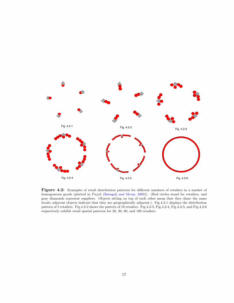
Fig. 4.2-1 Fig. 4.2-2 Fig. 4.2-3

Fig. 4.2-4 Fig. 4.2-5 Fig. 4.2-6

Figure 4.2: Examples of retail distribution patterns for different numbers of retailers in a market ofhomogeneous goods (plotted in Pajek (Batagelj and Mrvar, 2009)). (Red circles stand for retailers, andgray diamonds represent suppliers. Objects sitting on top of each other mean that they share the samelocale; adjacent objects indicate that they are geographically adjacent.). Fig.4.2-1 displays the distributionpattern of 5 retailers. Fig.4.2-2 shows the pattern of 10 retailers. Fig.4.2-3, Fig.4.2-4, Fig.4.2-5, and Fig.4.2-6respectively exhibit retail spatial patterns for 20, 30, 60, and 100 retailers.

17

0

200

400

600

800

1000

1200

1400

1 4 7 10 13 16 19 22 25 28 31 34 37 40 43 46 49 52 55 58 61 64 67 70 73 76 79 82 85 88 91 94 97 100

Dem

and 

Loca+on (1 to 100) 

Figure 4.3: Demand in different locations, with individuals’ demand following normal distribution (meanvalue equals 20 and st. dev. equals 10).

The above analysis indicates that when the number of retailers is no more than 10, the

centripetal force (proximity to suppliers) induces them to double up at supplier locales, while

the centrifugal force (proximity to customers) keeps the distribution pattern symmetric. As

the number of retailers continues to grow, retailers tend to disperse themselves along the

circle; the existence of centripetal force, however, keeps them near suppliers. Different

numbers of retailers in the competition beget different distribution patterns.

4.1.2 Heterogeneous population

What if individuals demands on product x are different? How would the final retail dis-

tribution patterns change? Here I test the scenario where individuals’ demand on product

x follows normal distribution, with average 20 and standard deviation 10; the number for

each consumer’s demand is randomly generated based on this distribution. There are 50

customers in each locale; the total demand in each location can be found in Fig. 4.3. The

high demand is equals 1171 at locale 78, and the lowest demand equals 830.

The find retail distribution pattern is shown in Fig. 4.4. Five symmetric retail clusters

show up around supplier locales; yet different from the previous result, the case where every

two retailers double up does not show up. The cluster density equals 1.

I further examine the case where the demand follows power-law distribution, assuming

that individual’s demand on product x ranges from 0 to 60 and that the scaling parameter

18

0

1

2

0 10 20 30 40 50 60 70 80 90 100

Number of retailers 

Loca1on (1 to 100) 

Figure 4.4: Retail distribution pattern in equilibrium, with individuals’ demand following normal dis-tribution.

equals -0.8. The demand distribution is shown in Fig. 4.5. The retail distribution pattern

in equilibrium, shown in Fig. 4.6, is the same as in Fig. 4.4. While each cluster’s locale is

slightly different, it covers a supplier locale. Retailers stay close to suppliers to minimize

costs and keep the density low to reach out to population with heterogeneous demand. It

further shows that heterogeneous population can impact retail location distribution.

4.1.3 Sensitivity tests

To further explore the effects of the centripetal and centrifugal forces on retail distribution

patterns, sensitivity tests are performed on β and u. When examining different values of β

or u, we set other parameters to be the same as in Table 4.1.

First, we test the value of β from 0 to 2.0 (with step size 0.25) and for each case run

the number of retailers from 2 to 30. Fig. 4.7 presents cluster densities for different values

of β. We observe that when β is larger than 0.5, retail distribution patterns are similar

to the base case (β = 1.0) described above. When β equals 0 or 0.25, retail geographical

distribution patterns considerably differ from other cases. When β equals 0, retailers are

evenly distributed and only locate in supplier locales for all scenarios of different numbers

of retailers. This is because as β equals 0, consumers are indifferent to travel and retailers

therefore stay at supplier locales to minimize cost. It is interesting to see that all retailers

19

0

200

400

600

800

1000

1200

1 4 7 10 13 16 19 22 25 28 31 34 37 40 43 46 49 52 55 58 61 64 67 70 73 76 79 82 85 88 91 94 97 100

Dem

and 

Loca+on (1 to 100) 

Figure 4.5: Demand in different locations, with individuals’ demand following power-law distribution(the scaling parameter equals -0.8).

0

1

2

0 10 20 30 40 50 60 70 80 90 100

Number of retailers 

Loca1on (1 to 100) 

Figure 4.6: Retail distribution pattern in equilibrium, with individuals’ demand following power-lawdistribution (the scaling parameter equals -0.8).

20

0

5

10

15

20

25

30

0 5 10 15 20 25 30

Cluster density

Number of retailers

beta = 0 beta = 0.25 beta = 0.5 beta = 0.75 beta = 1.0 beta = 1.25 beta = 1.5 beta = 2.0

Figure 4.7: Average cluster densities for the scenarios with retailers ranging from 2 to 30: results ofsensitivity tests on β (scaling parameter).

amass at only one supplier locale; cluster density therefore equals the number of retailers.

This is an artifact of the simulation model that retailers choose the first most profitable

locations and don’t consider alternative locations of exactly equal profits. They might just

as easily cluster uniformly or non-uniformly on any supplier locale.

I change the value of u from 0 to 0.16, with step size 0.02. Fig. 4.8 shows cluster densities

for different values of u. When u is larger than 0.08, retailers tend to double up on suppliers,

as their number booms from 2 to 10. However, as the number of retailers rises to 15, only

the case of u equaling 0.16 shows continuing accumulation of retailers at supplier locales,

which is different from the result of our base case (where u equals 0.02). In particular, in

the case of 15 retailers, every three retailers stay at a supplier locale. When u equals 0.16,

although the cluster density curve gradually falls as the number of retailers continues to

increase, a rising trend of cluster density can still be noticed when the number of retailers

ascends from 20 to 25.

I also examine the case where consumer demand can fluctuate. Since retailers’ sales price

is fixed, we relate consumer demand with retailers’ attractiveness. Consumer p’s demand

21

0 

0.5 

1 

1.5 

2 

2.5 

3 

3.5 

0  5  10  15  20  25  30  35 

Cluster density 

Number of retailers 

u = 0 

u = 0.02 

u = 0.04 

u = 0.06 

u = 0.08 

u = 0.10 

u = 0.12 

u = 0.16 

Figure 4.8: Average cluster densities for the scenarios with retailers ranging from 2 to 30: results ofsensitivity test on u (unit shipping cost).

on product x, λxp, is measured as:

λxp = α0 + α1 ·∑i∈Wx

eApi + εp (4.1)

Where∑

i∈WxeApi is a function of accessibility to retailers, as introduced in Eq.(2); the

error εp term is an i.i.d. with zero mean value. This expression originated from studies

on evaluating accessibility of location in transportation research (Ben-Akiva and Lerman,

1985). It indicates that the maximum utility of all alternatives in a choice set is a measure of

a consumer’s expected demand associated with this situation. While α0 and α1 are assumed

to be the same for all consumers, this function reflects the variation of the demands of

consumers in different locales and different rounds and for different scenarios.

In this simulation, α0 is set to be 10, representing a consumer’s basic demand on product

x; α1 equals 1.75, indicating a consumer’s demand elasticity with respect to accessibility

to retailers. Other parameters are the same as in Table 4.1. An increase of the number of

retailers generally induces the growing of consumers’ demand. Yet, here we set an upper

22

limit of 60 on an individual consumer’s demand on product x. We compare the results

of different numbers of retailers ranging from 2 to 100. The resultant retail distribution

pattern with elastic consumer demand is basically the same as the base case wherein demand

is inelastic.

Fig. 4.9 further shows the curve of individual consumer demand for different numbers of

retailers in the market. In the very beginning, consumers’ average demand gradually rises

with the increase of retailers; it stops growing when more than 26 retailers are in the game,

after it reaches the upper limit of individual consumer demand. It implies that as more

retailers partake in the competition, the implicit product and price differentiation as well as

the explicit lowered transportation costs increase demand in the first stage of the survival

curve of the product. Fig. 4.10 compares retail average profits with and without consumer

demand elasticity. We can see a steeper declining curve of average profits for the case with

consumer demand elasticity, which is a direct consequence of competition. The profit gap

is particularly salient when the number of retailers is between 5 and 40. As the number

of retailers continues to increase, the two curves get increasingly closer. The implication

is that as a new product is in its full swing of development in the market, a market with

consumer demand elasticity offers greater financial returns than one without. Yet, as the

product reaches its mature stage, retail profit decreases over time, and there is probably no

big difference between the market with demand elasticity and without demand elasticity.

4.2 The market of complementary goods

4.2.1 Base case

In the market of two complementary goods, we first examine the scenario of 10 suppliers

of x and 10 suppliers of y, every two of which co-locate and are evenly distributed around

the circle. Table 4.1 shows the values of the parameters used in this experiment (Model 2).

We first set 20 retailers (10 retailers of product x, 10 retailers of product y). Since multiple

equilibria are possible, 200 different retail initial location patterns (seeds) are examined.

Given different seeds, our model produces multiple stable patterns, which can be grouped

into three categories by the number of clusters (although each individual retailer’s final

23

0

10

20

30

40

50

60

70

0 10 20 30 40 50 60 70 80 90 100

Invidual consumer demand

Number of retailers

Figure 4.9: Individual consumer demand on product x increases with the rising of the number of retailers,yet does not exceed 60. When the number of retailers exceeds 26, average consumer demand reaches 60 (theupper limit of individual consumer demand) and stays constant thereafter.

0

20

40

60

80

100

120

0 10 20 30 40 50 60 70 80 90 100

Average retail profit ($1000)

Number of retailers

Market with demand elasticity

Market without demand elasticity

Figure 4.10: A comparison of retail average profit with and without consumer demand elasticity forthe number of retailers from 2 to 100. The curve of retail average profit without demand elasticity (basecase) goes under the curve with demand elasticity; the profit gap is particularly salient when the number ofretailers is between 5 and 40.

24

locale may vary in different outcomes). The most common pattern is only one cluster (with

probability 0.725), where all retailers accumulate at a supplier locale; the patterns of two

clusters and three clusters emerge with probability 0.24 and 0.036. All the retail distribution

patterns share two features: (1) retailers only stay at supplier locales; (2) the same number

of retailers of x and retailers of y co-locate, indicating that they constitute pairs. It is

interesting to notice that the evenly distributed pattern of retailers—every one retailer of x

and every one retailer of y double at a supplier locale—does not appear in this experiment.

To further explore this possibility, we intentionally set the initial distribution pattern to be

very similar to the evenly distributed one, which ultimately results in the evenly distributed

pattern of retailers.

4.2.2 Sensitivity tests

To understand the impact of the number of retailers on retail distribution patterns, we

further vary the total number of retailers from 4 to 40 while keeping the same number of

retailers of x and the number of retailers of y; other parameters are set to be the same as

the base case. After testing 200 seeds for each scenario, except for the case of 4 retailers,

our simulation results reveal multiple hierarchical retail distribution patterns for all cases.

Fig. 4.11 shows the probabilities for different retail clusters. It is interesting to notice that

the result of only one cluster has the highest probability to appear for all cases. Moreover,

by observing the trend of the histograms of one cluster for different numbers of retailers,

we can notice that the greater gap between the number of retailers and the number of

suppliers (which is 10 for each category of products), the more likely that all retailers tend

to accumulate in one cluster. The largest number of resultant clusters is 4; the probability

of its happenstance nonetheless never exceeds 0.05.

But what if we have different numbers of retailers of complementary goods? We vary

the number of retailers of product y from 2 to 16 while fixing the number of retailers of

x to be 10. 200 seeds are also tested for each scenario. The probability distribution for

different numbers of cluster is shown in Fig. 4.12. Overall, I find that the greater gap

between the number of retailers of product x and the number of retailers of y, the more

likely fewer clusters will emerge. Like the previous results, the case of one cluster has the

25

0

0.1

0.2

0.3

0.4

0.5

0.6

0.7

0.8

0.9

1

4 6 8 10 12 14 16 18 20 22 24 26 28 30 32 34 36 38 40

Probability

Number of retailers

1 cluster 2 clusters 3 clusters 4 clusters

Figure 4.11: Probability distribution of the numbers of clusters with retailers ranging from 4 to 40(where the number of retailers of x equals the number of retailers of y), with total 20 suppliers (10 suppliersof x and 10 suppliers of y). The case of one cluster has the highest probability to appear of all the cases.

highest probability to emerge and retailers only locate at supplier locales. Moreover, when

there are more than one cluster in a retail distribution pattern, the ratio of the number of

retailers of x to retailers of y in each cluster is very close. To illustrate, Fig. 4.13 shows

some retail distribution patterns for the case of 10 retailers of x and 15 retailers of y. Such

interesting phenomena may indicate that retailers of complementary goods can self-organize

themselves into clusters of similar structures.

26

0

0.1

0.2

0.3

0.4

0.5

0.6

0.7

0.8

0.9

1

2 3 4 5 6 7 8 9 10 11 12 13 14 15 16

Probability

Number of retailers of y

1 cluster 2 clusters 3 clusters 4 clusters 5 clusters

Figure 4.12: Probability distribution of the numbers of clusters with 10 retailers of product x and thenumber of retailers of product y ranging from 2 to 16 (shown in the horizontal axis). The case of only onecluster has the highest likelihood to emerge. The greater gap between the number of retailers of product xand the number of retailers of product y, the more likely that the case of fewer clusters will emerge.

27

!

9

!

6

!

!

Retail cluster of product x

Retail cluster of product y

Fig. 4.13-1 Fig. 4.13-2

Fig. 4.13-3 Fig. 4.13-4

Figure 4.13: Some retail distribution patterns (with more than one cluster) in equilibrium for 10 retailersof x and 15 retailers of y (plotted in Pajek (Batagelj and Mrvar, 2009)). A red circle stands for a retailcluster of x; a blue cross represents a retail cluster of y. Two shapes laid together show that they co-locate.The number in each shape indicates the number of retailers. All retailers stay at supplier locales. In Fig.4.13-1, the ratio of the number of retailers of x to the number of retailers of y for the two clusters respectivelyequals 3:5 and 7:10. In Fig.4.13-2, the ratios the number of retailers of x to the number of retailers of y forthe two clusters are identical, equaling 2:3. In Fig.4.13-3, the ratio respectively equals 3:5, 5:7, and 2:3 forthe three clusters. In Fig.4.13-4, the ratios for the three clusters are: 3:4, 3:5, and 4:6.

28

Chapter 5

Discussion and conclusions

5.1 Discussion

Our agent model in the market of homogeneous goods and the market of complementary

goods produces the emergence of retail clusters. In a market of homogeneous goods, clusters

tend to be symmetric. When retailers are few, they accumulate in suppliers’ locales; as the

number of retailers increases, they spread out around suppliers and incrementally occupy

the whole circle. Moreover, a larger scaling parameter (absolute) value for consumers tends

to make the retail pattern more spread out, and higher unit shipping cost makes retailers

more concentrated around suppliers. Such results exhibit the balance between proximity to

the market and proximity to suppliers which impacts the retail distribution pattern.

In the market of two complementary goods, multiple equilibria of retail distribution

patterns are found to be common; nevertheless, the case of only one cluster—where all

retailers accumulate in a supplier locale—is most likely to emerge. Moreover, the greater gap

between the number of retailers of x and the number of retailers of y, the more likely dense

clusters are to emerge. A further extrapolation suggests that in the market of homogeneous

goods, the case of one cluster cannot be stable in that some retailers in the big cluster can

easily move to an open space on the circle to occupy a larger market. In the model of

complementary goods, however, since consumers consider total travel distance for buying

both goods, retail location choice depends not only on their distance to suppliers and

consumers, but also on their distance to retailers of complementary goods. Additionally, for

29

the patterns with more than one cluster, our results imply that emergent clusters, however

different in size, tend to have a similar composition in terms of the ratio of retailers of

complementary goods.

In central place theory, Christaller (1933) claimed that in the areas with population and

resources which are evenly distributed, settlements have equidistant spacing between centers

of the same order; high-order services are farther away from low-order services. Yet, this

research demonstrates that even in a market of two equally important products, hierarchical

distribution patterns can also autonomously emerge. This comports with the notion of retail

districts found in many cities, such as the Kappabashi district of Tokyo specializing in

kitchen equipment (and plastic sushi) along with similar examples of clustered competitors

(Levinson and Krizek, 2008). In our model of complementary goods, although the evenly-

distributed pattern of retailers can occur under certain circumstances, to achieve this each

cluster requires a very specific timing, which has a high requirement for initial seeds and

the sequence of location choice. Therefore it is much less likely to naturally emerge than

the hierarchical patterns. Overall, our results find autonomous emergence of retail clusters;

the hierarchical distribution patterns (in particular, the pattern of only one cluster) appear

with a high probability.

5.2 Conclusion

This thesis builds an agent-based model to examine retail location choice on a supply chain

network of consumers, retailers, and suppliers. In a market of homogeneous goods, we find

symmetric retail distribution patterns, and average cluster density changes dynamically as

retailers join the market. These patterns are affected by shipping cost and consumers’

willingness to travel. Our findings demonstrate that the development of a market does

not always lead to condensed agglomeration of business locations. Moreover, the balance

between transportation cost and market size considerably impacts the size and density of

clusters.

In a market of two complementary goods, assuming suppliers of the two products co-

locate and evenly distribute themselves, we find self-organizing retail clusters with features

different from the results of the first model. First, multiple equilibria of retail distributions

30

are common. Second, co-locating of retailers of complementary goods appears with a high

probability. Moreover, the likelihood of clustering increases with the gap between the

number of retailers of complementary goods and the gap between the number of retailers

and the number of suppliers. Third, when more than one cluster occurs, however different

in size, the ratio of the number of retailers of one product to the number of retailers of

the other product tends to be close for the emergent clusters. Our results illustrate that

competition among retailers on supply chains (especially when considering trip chaining for

complementary goods on the part of the customer) is sufficient to produce clustering, and

other mechanisms (such as the desire of customers to comparison shop) are not required,

but may also be additional source of clustering behavior. We have not identified whether

there is a necessary assumption to produce clustering.

Future research should address the efficiency of such self-organized retail patterns in

terms of social welfare, as opposed to a more evenly distributed one (such as posited in

central place theory). Empirical studies should also test the hypotheses presented in this

research.

31

Bibliography

Andersson, C., Frenken, K. and Hellervik, A. (2006), “A complex network approach tourban growth”, Environment and Planning A , Vol. 38, p. 1941.

Applebaum, W. (1940), “How to Measure the Value of a Trading Area”, Chain Store Age ,Vol. Nov., pp. 111–114.

Applebaum, W. (1960), “Methods for determining store trading areas, market penetrationand potential sales”, Journal of Marketing Research , Vol. 3, pp. 127–41.

Arthur, W. B. (1989), Urban systems and historical path dependence, in R. Herman andJ. Ausubel, eds, ‘Urban Systems and Infrastructure’, National Academy of Sciences.

Arthur, W. B. (1990), “Positive feedbacks in the economy”, Scientific American , Vol. 262,pp. 92–99.

Bacon, R. (1984), Consumer Spatial Behavior: A Model of Purchasing Decisions over Spaceand Time, Oxford: Claredon.

Batagelj, V. and Mrvar, A. (2009), ‘Networks/Pajek Program for Large Network Analysis’,http://vlado.fmf.uni-lj.si/pub/networks/pajek.

Batty, M. (1991), Cities as fractals: simulating growth and form, in R. E. T. Crilly andH. Jones, eds, ‘Fractals and Chaos’, New York: Springer-Verlag.

Batty, M. and Rana, S. (2004), “The automatic definition and generation of axial lines andaxial maps”, Environment and Planning B , Vol. 31, pp. 615–640.

Batty, M. and Xie, Y. (1999), “Self-organized criticality and urban development”, DiscreteDynamics in Nature and Society , Vol. 3, pp. 109–124.

Ben-Akiva, M. E. and Lerman, S. R. (1985), Discrete Choice Analysis: Theory and Appli-cation to Travel Demand, MIT Press.

Berger, T. (2001), “Agent-based spatial models applied to agriculture: a simulation tool fortechnology diffusion, resource use changes and policy analysis”, Agricultural Economics ,Vol. 25, pp. 245–260.

Berger, T. and Ringler, C. (2002), “Tradeoffs, efficiency gains and technical change- Mod-eling water management and land use within a multiple-agent framework”, QuarterlyJournal of International Agriculture , Vol. 41, pp. 119–144.

32

Boschma, R. and Frenken, K. (2006), “Why is economic geography not an evolutionaryscience? Towards an evolutionary economic geography”, Journal of Economic Geography, Vol. 6, pp. 273–302.

Brown, D., Page, S., Riolo, R., Zellner, M. and Rand, W. (2005), “Path dependence andthe validation of agent-based spatial models of land use”, International Journal of Geo-graphical Information Science , Vol. 19, pp. 153–174.

Brown, S. (1989), “Retail Location Theory: The Legacy of Harold Hotelling”, Journal ofRetailing , Vol. 65, pp. 450–70.

Christaller, W. (1933), Die zentralen Orte in Suddeutschland, Gustav Fischer Varlag, Jena.English translation: The Central Places of Southern Germany. (1966) Prentice-Hall, En-glewood Cliffs, NJ.

Clarke, I., Hallsworth, A., Jackson, P., De Kervenoael, R., Del Aguila, R. and Kirkup, M.(2006), “Retail restructuring and consumer choice 1. Long-term local changes in consumerbehaviour: Portsmouth, 1980-2002”, Environment and Planning A , Vol. 38, pp. 25–46.

Dale, B. and Sjoholt, P. (2007), “The changing structure of the central place system inTrondelag, Norway, over the past 40 years-viewed in the light of old and recent theoriesand trends”, Geography Annuals B , Vol. 89, BLACKWELL PUBLISHERS, p. 13.

d’Aspremont, C., Gabszewicz, J. and Thisse, J. (1979), “On Hotelling’s stability in compe-tition”, Econometrica , Vol. 47, pp. 1145–1150.

Davies, R. and Rogers, D. (1984), Store Location and Store Assessment Research, N.Y.:Wiley.

de la Barra, T., Perez, B. and Vera, N. (1984), “TRANUS-J: putting large models into smallcomputers”, Environment and Planning B: Planning and Design , Vol. 11, pp. 87–101.

Eaton, B. and Lipsey, R. (1982), “An economic theory of central places”, Economic Journal, Vol. 92, pp. 56–72.

Evans, T. and Kelley, H. (2004), “Multi-scale analysis of a household level agent-basedmodel of landcover change”, Journal of Environmental Management , Vol. 72, pp. 57–72.

Frankowiak, E. (1978), “Location Perception and the Hierarchical Structure of Retail Cen-ters”, University of Michigan Geographical Publication , Vol. 22.

Friedmann, J. (1986), “World city hypothesis”, Development and Change , Vol. 17, pp. 69–83.

Fujita, M. and Ogawa, H. (1982), “Multiple equilibria and structural transition of non-monocentric urban configurations”, Regional Science and Urban Economics , Vol. 12,pp. 161–196.

Fujita, M., Ogawa, H. and Thisse, J. (1988), “A spatial competition approach to centralplace theory: some basic principles”, Journal of Regional Science , Vol. 28, pp. 477–494.

33

Gabaix, X. and Ioannides, Y. (2004), “The Evolution of City Size Distributions”, Handbookof Regional and Urban Economics , Vol. 4, pp. 2341–2378.

Halperin, W. C., Gale, N., Golledge, R. and Hubert, L. (1983), “Exploring EntrepreneurialCognitions of Retail Environments”, Economic Geography , Vol. 59, Clark University,pp. 3–15.

Handy, S. (1996), “Understanding the link between urban form and nonwork travel behav-ior”, Journal of Planning Education and Research , Vol. 15, ACSP, p. 183.

Handy, S., Cao, X. and Mokhtarian, P. (2005), “Correlation or causality between the builtenvironment and travel behavior? Evidence from Northern California”, TransportationResearch Part D , Vol. 10, Elsevier, pp. 427–444.

Handy, S., Mokhtarian, P., Buehler, T. and Cao, X. (2004), “Residential location choiceand travel behavior: Implications for air quality”, Report for the California Departmentof Transportation, Davis, CA .

Hill, D. M., Brand, D. and Hansen, W. B. (1966), “Prototype development of a statisticalland use prediction model for the Greater Boston Region”, Highway Research Board ,Vol. 114, pp. 51–70.

Hotelling, H. (1929), “Stability in competition”, Economic Journal , Vol. 39, pp. 41–57.

Huff, D. (1964), “Defining and estimating a trading area”, The Journal of Marketing ,Vol. 39, pp. 41–57.

Huff, D. L. and Rust, R. T. (1984), “Measuring the congruence of market areas”, TheJournal of Marketing , Vol. 48, American Marketing Association, pp. 68–74.

Hunt, J. D. and Simmonds, D. C. (1993), “Theory and application of an integrated land useand transport modelling framework”, Environment and Planning B , Vol. 20, pp. 221–221.

Ingram, G., Kain, J. F. and Ginn, J. R. (1972), The Detroit prototype of the NBER urbansimulation model, New York: Columbia University Press.

Jackson, P., Del Aguila, R., Clarke, I., Hallsworth, A., De Kervenoael, R. and Kirkup, M.(2006), “Retail restructuring and consumer choice 2. Understanding consumer choice atthe household level”, Environment and Planning A , Vol. 38, pp. 47–67.

Jacobs, J. (1961), The Death and Life of Great American Cities, New York: Vintage Books,Random House.

Jones, K. G. and Simmons, J. W. (1990), The Retail Environment, Van Nostrand Reinhold.

Krugman, P. R. (1991), Geography and Trade, Cambridge: MIT Press.

Krugman, P. R. (1996), “Urban concentration: the role of increasing returns and transportcosts”, International Regional Science Review , Vol. 19, pp. 5–30.

Landis, J. D. (1994), “The California urban futures model: a new generation of metropolitansimulation models”, Environment and Planning B , Vol. 21, pp. 399–399.

34

Landis, J. D. and Zhang, M. (1998), “The second generation of the California urban futuresmodel. Part 1: Model logic and theory”, Environment and Planning B , Vol. 25, pp. 657–666.

Laulajainen, R. (1987), Spatial strategies in retailing, D Reidel Pub Co.

Leitham, S., McQuaid, R. and Nelson, J. (2000), “The influence of transport on indus-trial location choice: a stated preference experiment”, Transportation Research Part A ,Vol. 34, Elsevier, pp. 515–535.

Levinson, D. and Krizek, K. (2008), Planning for Place and Plexus : Metropolitan LandUse and Transport, New York, NY: Routledge.

Levinson, D., Xie, F. and Zhu, S. (2007), “The co-evolution of land use and road networks”,Proceedings of the 17th International Symposium on Transportation and Traffic Theory(ISTTT) .

Losch, A. (1940), Die raumliche Ordnung der Wirtschaft, Fischer, Jena. English translation:The Economies of Location (1954) New Haven, CT: Yale University Press.

Manson, S. M. (2000), Agent-based dynamic spatial simulation of land-use/cover change inthe Yucatan peninsula, Mexico, in ‘Fourth International Conference on Integrating GISand Environmental Modeling (GIS/EM4), Banff, Canada’, pp. 2–8.

Marshall, A. (1890), Principles of Economics, London Macmillan (8th ed. in 1920).

Martin, R. and Sunley, P. (2006), “Path dependence and regional economic evolution”,Journal of Economic Geography , Vol. 6, pp. 395–437.

Ottaviano, G. I. P. and Puga, D. (1998), “Agglomeration in the global economy: a surveyof the new economic geography”, The World Economy , Vol. 21, pp. 707–731.

Parker, D. and Filatova, T. (2008), “A conceptual design for a bilateral agent-based landmarket with heterogeneous economic agents”, Computers, Environment and Urban Sys-tems , Vol. 32, pp. 454–463.

Parker, D., Manson, S., Janssen, M., Hoffmann, M. and Deadman, P. (2003), “Multi-agentsystems for the simulation of land-use and land-cover change: a review”, Annals of theAssociation of American Geographers , Vol. 93, pp. 314–337.

Peponis, J., Wineman, J., Bafna, S., Rashid, M. and Kim, S. (1998), “On the generation oflinear representations of spatial configuration”, Environment and Planning B , Vol. 25,pp. 559–576.

Porter, M. (1990), “The competitve advantage of nations”, Harvard Business Review ,pp. 73–93.

Portugali, J. (1999), Self-Organization and the City, Berlin: Springer.

Putman, S. H. (1991), Integrated urban models 2: new research and applications of opti-mization and dynamics, London: Pion.

35

Quinzii, M. and Thisse, J. (1990), “On the optimality of central places”, Econometrica ,Vol. 58, pp. 1101–1119.

Sanders, L., Pumain, D., Mathian, H., Guerin-Pace, F. and Bura, S. (1997), “SIMPOP: amultiagent system for the study of urbanism”, Environment and Planning B , Vol. 24,pp. 287–306.

Sassen, S. (1991), The Global City, Princeton, NJ: Princeton University Press.

Schwanen, T., Dijst, M. and Dieleman, F. (2004), “Policies for urban form and their impacton travel: the Netherlands experience”, Urban Studies , Vol. 41, p. 579.

Scott, A. (1988), Metropolis: From the Division of Labor to Urban Form, University ofCalifornia Press.

Targa, F. and Clifton, K.and Mahmassani, H. (2006), “Influence of Transportation Accesson Individual Firm Location Decisions”, Transportation Research Record , Vol. 1977,Transportation Research Board, pp. 179–189.

Taylor, P. (2004), World City Network: A Global Urban Analysis, London; New York:Routledge.

von Thunen, J. H. (1826), Der isolierte Staat in Beziehung auf Landwirtschaft und Na-tionalokonomie, 1, Hamburg: Perthes. English Translation: Wartenberg, CM (1966) vonThunen’s Isolated State. Oxford: Pergamon Press.

Waddell, P. (2002), “Modeling urban development for land use, transportation, and envi-ronmental planning”, Journal of the American Planning Association , Vol. 68.

Waddell, P., Borning, A., Noth, M., Freier, N., Becke, M. and Ulfarsson, G. (2003), “Mi-crosimulation of urban development and location choices: design and implementation ofurbanSim”, Networks and Spatial Economics , Vol. 3, Springer, pp. 43–67.

Weber, A. (1909), uber den Standort der Industrien., Mohr, Tubingen. English translation:Theory of the Location of Industries (1929) Chicago: University of Chicago Press.

Webster, C. (2003), “The nature of the neighborhood”, Urban Studies , Vol. 40, pp. 2591–2612.

Wegener, M. (2004), Overview of land use transport models, in D. A. Hensher, K. J.Button, K. E. Haynes and P. Stopher, eds, ‘Handbook of Transport Geography andSpatial Systems’, Vol. 5, Elsevier.

Wu, F. and Webster, C. (1998), “Simulation of natural land use zoning under free-marketand incremental development control regimes”, Computers, Environment and Urban Sys-tems , Vol. 22, pp. 241–256.

Wu, F. and Webster, C. (2000), “Simulating artificial cities in a GIS environment: ur-ban growth under alternative regulation regimes”, International Journal of GeographicalInformation Science , Vol. 14, pp. 625–648.

Yim, Y. (1993), Shopping trips and spatial distribution of food stores. University of Cali-fornia Transportation Center Working Paper: UCTC No. 125.

36