Why is Spatial Stereoacuity so Poor? Martin S. Banks School of Optometry, Dept. of Psychology UC...
64
hy is Spatial Stereoacuity so Poor Martin S. Banks School of Optometry, Dept. of Psychology UC Berkeley Sergei Gepshtein Vision Science Program UC Berkeley Michael S. Landy Dept. of Psychology, Center for Neural Science NYU Supported by NIH
-
date post
21-Dec-2015 -
Category
Documents
-
view
214 -
download
0
Transcript of Why is Spatial Stereoacuity so Poor? Martin S. Banks School of Optometry, Dept. of Psychology UC...

Why is Spatial Stereoacuity so Poor?Why is Spatial Stereoacuity so Poor?
Martin S. BanksSchool of Optometry, Dept. of Psychology
UC Berkeley
Sergei GepshteinVision Science Program
UC Berkeley
Michael S. LandyDept. of Psychology, Center for Neural Science
NYU
Supported by NIH

Depth Perception

Depth Perception
How precise is the depth map generated from disparity?

Precision of Stereopsis
Stereo precision measured in various waysA: Precision of detecting depth change on line of sightD: Precision of detecting spatial variation in depth
from Tyler (1977)

Precision of Stereopsis
Stereo precision measured in various waysA: Detect depth change on line of sightD: Precision of detecting spatial variation in depth
from Tyler (1977)

Precision of Stereopsis
Stereo precision measured in various waysA: Detect depth change on line of sightD: Detect spatial variation in depth
from Tyler (1977)

Spatial Stereoacuity
• Modulate disparity sinusoidally creating corrugations in depth.
• Least disparity required for detection as a function of spatial frequency of corrugations: “Disparity MTF”.
• Index of precision of depth map.

Disparity MTF
•Disparity modulation threshold as a function of spatial frequency of corrugations.
•Bradshaw & Rogers (1999).
•Horizontal & vertical corrugations.
•Disparity MTF: acuity = 2-3 cpd; peak at 0.3 cpd.

Luminance Contrast Sensitivity & Acuity
• Luminance contrast sensitivity function (CSF): contrast for detection as function of spatial frequency.
• Proven useful for characterizing limits of visual performance and for understanding optical, retinal, & post-retinal processing.
• Highest detectable spatial frequency (grating acuity): 40-50 c/deg.
Disparity MTF
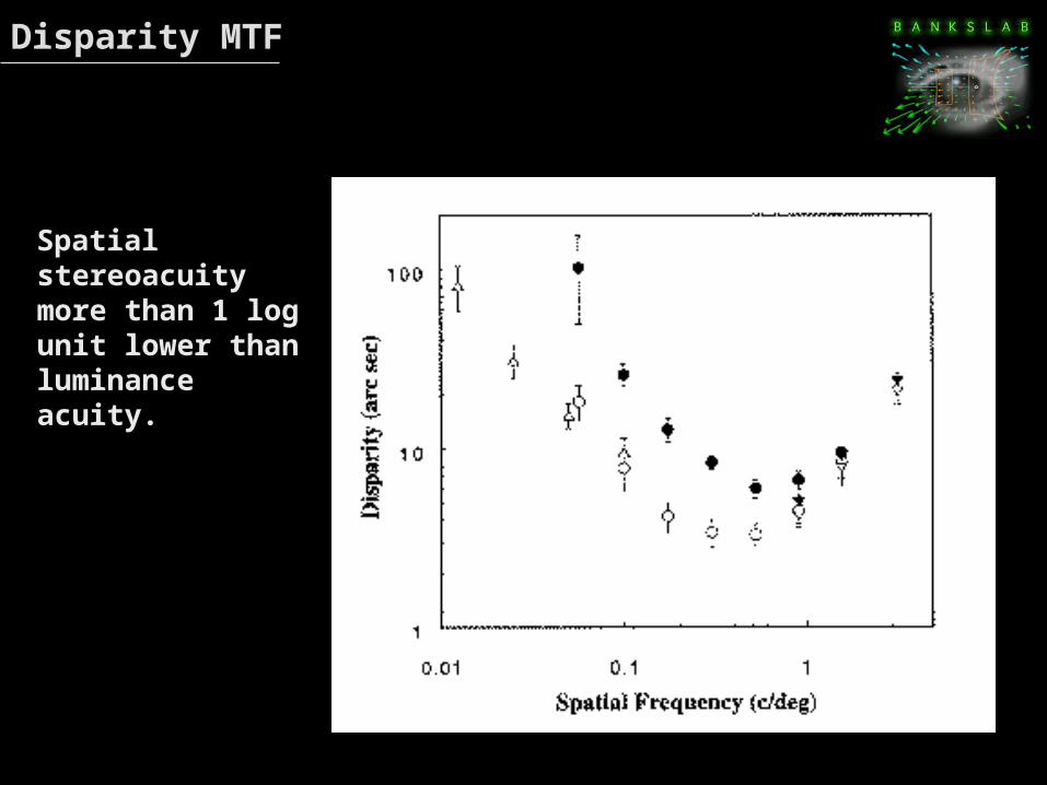
Spatial stereoacuity more than 1 log unit lower than luminance acuity.

Disparity MTF
Why is spatial stereoacuity so low?
Spatial stereoacuity more than 1 log unit lower than luminance acuity.
Likely Constraints to Spatial Stereoacuity
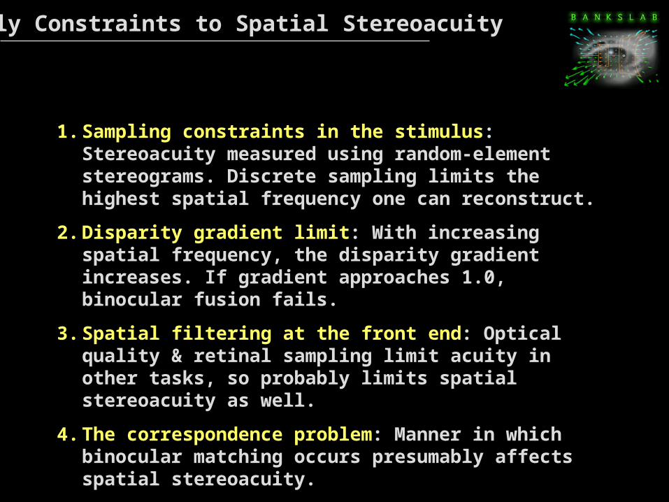
1. Sampling constraints in the stimulus: Stereoacuity measured using random-element stereograms. Discrete sampling limits the highest spatial frequency one can reconstruct.
2. Disparity gradient limit: With increasing spatial frequency, the disparity gradient increases. If gradient approaches 1.0, binocular fusion fails.
3. Spatial filtering at the front end: Optical quality & retinal sampling limit acuity in other tasks, so probably limits spatial stereoacuity as well.
4. The correspondence problem: Manner in which binocular matching occurs presumably affects spatial stereoacuity.

Likely Constraints to Spatial Stereoacuity
1. Sampling constraints in the stimulus: Stereoacuity measured using random-element stereograms. Discrete sampling limits the highest spatial frequency one can reconstruct.
2. Disparity gradient limit: With increasing spatial frequency, the disparity gradient increases. If gradient approaches 1.0, binocular fusion fails.
3. Spatial filtering at the front end: Optical quality & retinal sampling limit acuity in other tasks, so probably limits spatial stereoacuity as well.
4. The correspondence problem: Manner in which binocular matching occurs presumably affects spatial stereoacuity.

Spatial Sampling Limit: Nyquist Frequency
• Signal reconstruction from discrete samples.
• At least 2 samples required per cycle.
• In 1d, highest recoverable spatial frequency is Nyquist frequency:
where N is number of samples per unit distance.
1
2Nf N

Spatial Sampling Limit: Nyquist Frequency
• Signal reconstruction from 2d discrete samples.
• In 2d, Nyquist frequency is:
where N is number of samples in area A.
1
2N
Nf
A

Methodology
• Random-dot stereograms with sinusoidal disparity corrugations.
• Corrugation orientations: +/-20 deg (near horizontal).
• Observers identified orientation in 2-IFC psychophysical procedure; phase randomized.
• Spatial frequency of corrugations varied according to adaptive staircase procedure.
• Spatial stereoacuity threshold obtained for wide range of dot densities.
• Duration = 600 msec; disparity amplitude = 16 minarc.

Stimuli

Spatial Stereoacuity as a function of Dot Density
Dot Density (dots/deg2)
Sp
atia
l S
tere
oac
uit
y (c
/deg
)
•Acuity proportional to dot density squared.
•Scale invariance!
•Asymptote at high density.
0.1
1.0
ModulationAmplitude
ViewingDistance
16 min 39 cm
JMA MSB
DMV TMG
0.1 1.0 10 100 0.1 1.0 10 1000.1
1.0
a d
1
0.1
1
0.110.1 10 100 10.1 10 100

• Calculated Nyquist frequency for our displays.
Dot Density (dots/deg2)
Sp
atia
l S
tere
oac
uit
y (c
/deg
)
0.1
1.0
ModulationAmplitude
ViewingDistance
16 min 39 cm
JMA MSB
DMV TMG
0.1 1.0 10 100 0.1 1.0 10 1000.1
1.0
1
0.1
1
0.110.1 10 100 10.1 10 100
Spatial Stereoacuity & Nyquist Limit
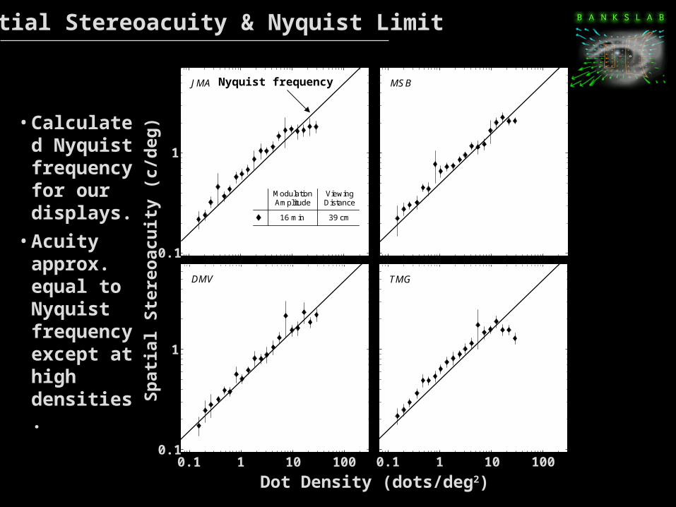
• Calculated Nyquist frequency for our displays.
• Acuity approx. equal to Nyquist frequency except at high densities.
Dot Density (dots/deg2)
Sp
atia
l S
tere
oac
uit
y (c
/deg
)
0.1
1.0
ModulationAmplitude
ViewingDistance
16 min 39 cm
JMA MSB
DMV TMG
0.1 1.0 10 100 0.1 1.0 10 1000.1
1.0
1
0.1
1
0.110.1 10 100 10.1 10 100
Spatial Stereoacuity & Nyquist Limit
Nyquist frequency

Types of Random-element Stereograms
Jittered-lattice: dots displaced randomly from regular lattice
Sparse random: dots positioned randomly

Spatial Sampling Limit: Nyquist Frequency
Same acuities with jittered-lattice and sparse random stereograms.
Both follow Nyquist limit at low densities.

Likely Constraints to Spatial Stereoacuity
1. Sampling constraints in the stimulus: Stereoacuity measured using random-element stereograms. Discrete sampling limits the highest spatial frequency one can reconstruct.
2. Disparity gradient limit: With increasing spatial frequency, the disparity gradient increases. If gradient approaches 1.0, binocular fusion fails.
3. Spatial filtering at the front end: Optical quality & retinal sampling limit acuity in other tasks, so probably limits spatial stereoacuity as well.
4. The correspondence problem: Manner in which binocular matching occurs presumably affects spatial stereoacuity.

Disparity Gradient
P1
P2
L R
Disparity gradient = disparity / separation
= (R – L) / [(L + R)/2]
Disparity Gradient
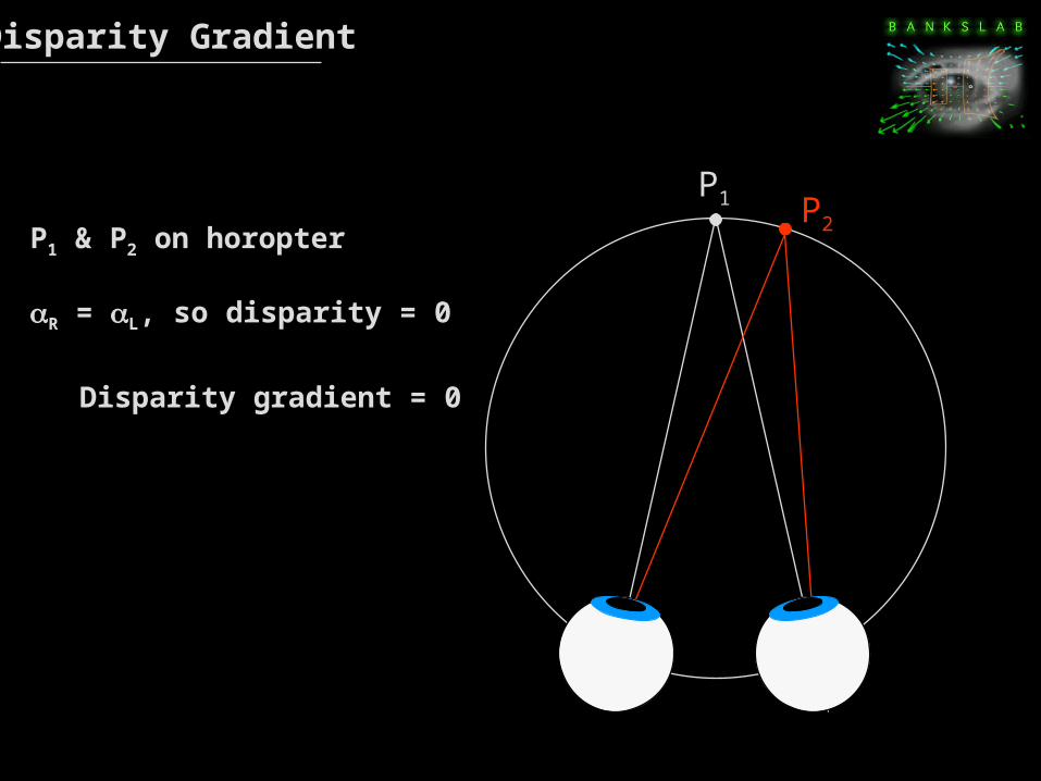
Disparity gradient = 0
P1 & P2 on horopter
R = L, so disparity = 0
P1 P2

Disparity Gradient
Disparity gradient =
P1 & P2 on cyclopean line of sight
R = -L, so separation = 0
P1
P2

Disparity Gradient
Disparity gradient for different directions.
horizontaldisparity
sepa
ratio
n
P1
P2 (left & right
eyes)

Disparity Gradient Limit
• Burt & Julesz (1980): fusion as function of disparity, separation, & direction (tilt).
• Set direction & horizontal disparity and found smallest fusable separation.
disparity
sepa
ratio
n
P1
P2 (left & right eyes)
direction

Disparity Gradient Limit
• Fusion breaks when disparity gradient reaches constant value.
• Critical gradient = ~1.
• “Disparity gradient limit”.
• Limit same for all directions.

Disparity Gradient Limit

Disparity Gradient Limit
• Panum’s fusion area (hatched).
• Disparity gradient limit means that fusion area affected by nearby objects (A).
• Forbidden zone is conical (isotropic).
Horizontal Position (deg)
Dis
par
ity
(deg
)
highest gradient
peak-trough gradient
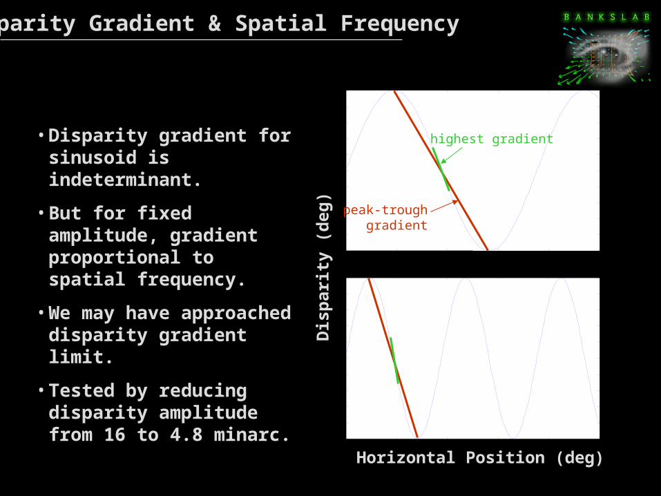
Disparity Gradient & Spatial Frequency
• Disparity gradient for sinusoid is indeterminant.
• But for fixed amplitude, gradient proportional to spatial frequency.
• We may have approached disparity gradient limit.
• Tested by reducing disparity amplitude from 16 to 4.8 minarc.

Spatial Stereoacuity & Disparity Gradient Limit
• Reducing disparity amplitude increases acuity at high dot densities (where DG is high).
• Lowers acuity slightly at low densities (where DG is low).
0.1
1.0
ModulationAmplitude
ViewingDistance
39 cm4.8 min
16 min 39 cm
JMA MSB
DMV TMG
0.1 1.0 10 100 0.1 1.0 10 1000.1
1.0
Nyquist frequency
Dot Density (dots/deg2)
Sp
atia
l S
tere
oac
uit
y (c
/deg
)
1
0.1
1
0.110.1 10 100 10.1 10 100

Likely Constraints to Spatial Stereoacuity
1. Sampling constraints in the stimulus: Stereoacuity measured using random-element stereograms. Discrete sampling limits the highest spatial frequency one can reconstruct.
2. Disparity gradient limit: With increasing spatial frequency, the disparity gradient increases. If gradient approaches 1.0, binocular fusion fails.
3. Spatial filtering at the front end: Optical quality & retinal sampling limit acuity in other tasks, so probably limits spatial stereoacuity as well.
4. The correspondence problem: Manner in which binocular matching occurs presumably affects spatial stereoacuity.

Stereoacuity & Front-end Spatial Filtering
• Low-pass spatial filtering at front-end of visual system determines high-frequency roll-off of luminance CSF.
• Tested similar effects on spatial stereoacuity by:
1. Decreasing retinal image size of dots by increasing viewing distance.
2. Measuring stereoacuity as a function of retinal eccentricity.
3. Measuring stereoacuity as a function of blur.

Spatial Stereoacuity at Higher Densities
• Monocular artifacts at high dot densities.
• Reduce dot size to test upper limit.
• Increase viewing distance from 39-154 cm.
• Acuity still levels off, but at higher value.
0.1
1.0
JMA MSB
Spa
tialS
tere
oa
cuity
(c/d
eg)
DMV TMG
Dot Density (dot/deg2)
0.1 1.0 10 100 0.1 1.0 10 1000.1
1.0
ModulationAmplitude
ViewingDistance
39 cm4.8 min
154 cm4.8 min
Nyquist frequency
Dot Density (dots/deg2)
Sp
atia
l S
tere
oac
uit
y (c
/deg
) 1
0.1
1
0.110.1 10 100 10.1 10 100

Stereoacuity & Front-end Spatial Filtering
• Low-pass spatial filtering at front-end of visual system determines high-frequency roll-off of luminance CSF.
• Tested similar effects on spatial stereoacuity by:
1. Decreasing retinal image size of dots by increasing viewing distance.
2. Measuring stereoacuity as a function of retinal eccentricity.
3. Measuring stereoacuity as a function of blur.
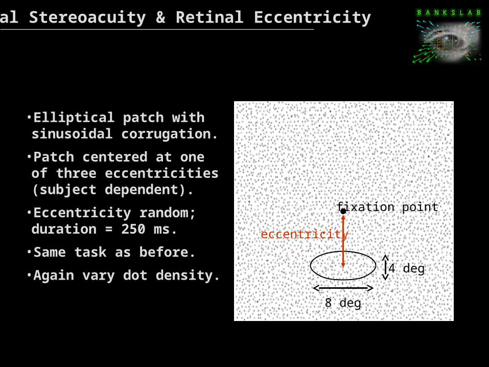
Spatial Stereoacuity & Retinal Eccentricity
8 deg
4 deg
fixation point
eccentricity
•Elliptical patch with sinusoidal corrugation.
•Patch centered at one of three eccentricities (subject dependent).
•Eccentricity random; duration = 250 ms.
•Same task as before.
•Again vary dot density.

Spatial Stereoacuity & Retinal Eccentricity

Spatial Stereoacuity & Retinal Eccentricity
0.1
1.0
TMG
0.1 1.0 10 100
YHH
1.0 10 100 1.0 10 100
SSG
Dot Density (dots/deg2)
Sp
atia
l S
tere
oac
uit
y (c
/deg
)
0 deg
5.2
10.4
0 deg
6.2
12.4
0 deg
6.8
13.6
Retinal eccentricity
•Same acuities at low dot densities; Nyquist.
•Asymptote varies significantly with retinal eccentricity.
1
0.1
10.1 10 100 1 10 100 1 10 100

Stereoacuity & Front-end Spatial Filtering
• Low-pass spatial filtering at front-end of visual system determines high-frequency roll-off of luminance CSF.
• Tested similar effects on spatial stereoacuity by:
1. Decreasing retinal image size of dots by increasing viewing distance.
2. Measuring stereoacuity as a function of retinal eccentricity.
3. Measuring stereoacuity as a function of blur.

Spatial Stereoacuity & Blur
• We examined effect of blur on foveal spatial stereoacuity.
• Three levels of blur introduced with diffusion plate:
no blur ( = 0 deg)low blur ( = 0.12)high blur ( = 0.25)

Spatial Stereoacuity & Blur
• We examined effect of blur on foveal spatial stereoacuity.
• Three levels of blur introduced with diffusion plate:
no blur ( = 0 deg)low blur ( = 0.12)high blur ( = 0.25)

Spatial Stereoacuity & Blur
•Same acuities at low dot densities; Nyquist.
•Asymptote varies significantly with spatial lowpass filtering.

Likely Constraints to Spatial Stereoacuity
1. Sampling constraints in the stimulus: Stereoacuity measured using random-element stereograms. Discrete sampling limits the highest spatial frequency one can reconstruct.
2. Disparity gradient limit: With increasing spatial frequency, the disparity gradient increases. If gradient approaches 1.0, binocular fusion fails.
3. Spatial filtering at the front end: Optical quality & retinal sampling limit acuity in other tasks, so probably limits spatial stereoacuity as well.
4. The correspondence problem: Manner in which binocular matching occurs presumably affects spatial stereoacuity.

Binocular Matching by Correlation
1. Binocular matching by correlation: basic and well-studied technique for obtaining depth map from binocular images.
Computer vision: Kanade & Okutomi (1994); Panton (1978)
Physiology: Ohzawa, DeAngelis, & Freeman (1990); Cumming & Parker (1997)
2. We developed a cross-correlation algorithm for binocular matching & compared its properties to the psychophysics.

Left eye’s image Right eye’s image
• Compute cross-correlation between eyes’ images.
• Window in left eye’s image moved orthogonal to signal.
• For each position in left eye, window in right eye’s image moved horizontally & cross-correlation computed.
Binocular Matching by Correlation

Left eye’s image Right eye’s image
• Compute cross-correlation between eyes’ images.
• Window in left eye’s image moved orthogonal to signal.
• For each position in left eye, window in right eye’s image moved horizontally & cross-correlation computed.
Binocular Matching by Correlation

Left eye’s image Right eye’s image
• Compute cross-correlation between eyes’ images.
• Window in left eye’s image moved orthogonal to signal.
• For each position in left eye, window in right eye’s image moved horizontally & cross-correlation computed.
Binocular Matching by Correlation

Binocular Matching by Correlation
Plot correlation as a function of position in left eye (red arrow) & relative position in right eye (blue arrow); disparity.
Correlation (gray value) high where images similar & low where dissimilar.
X axis
Y axis
Position in left eye’s image
Po
siti
on
in r
igh
t ey
e’s
imag
e

0.1 1 10 100
Dot Density
Sp
atia
l F
req
uen
cy
1
0.1
Examples of Output
Dot density: 16 dots/deg2
Spatial frequency: 1 c/degWindow size: 0.2 deg
Disparity waveform evident in output
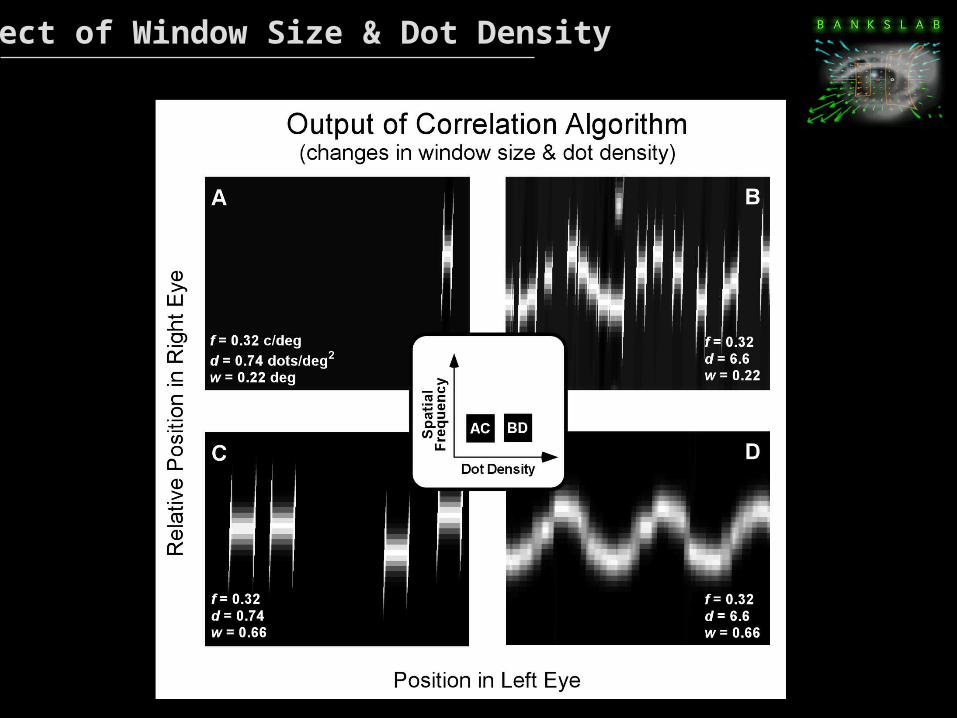
Effect of Window Size & Dot Density

Effect of Window Size & Dot Density
2 0 7.w d
Correlation window must be large enough to contain sufficient luminance variation to find correct matches

Effect of Window Size & Spatial Frequency

Effect of Window Size & Spatial Frequency
0 5.w f
When significant depth variation is present in a region, window must be small enough to respond differentially

Window Size, # Samples, & Spatial Frequency
0 5.w f
2 0 7.w d From two constraints:
then substitute for w, take log:
10 22
2log log .f d
Effect of Disparity Gradient
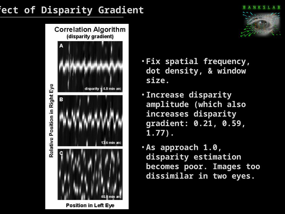
• Fix spatial frequency, dot density, & window size.
• Increase disparity amplitude (which also increases disparity gradient: 0.21, 0.59, 1.77).
• As approach 1.0, disparity estimation becomes poor. Images too dissimilar in two eyes.
• Matching by correlation yields piecewise frontal estimates.

Effect of Disparity Gradient
• Fix spatial frequency, dot density, & window size.
• Increase disparity amplitude (which also increases disparity gradient: 0.21, 0.59, 1.77).
• As approach 1.0, disparity estimation becomes poor. Images too dissimilar in two eyes.
• Matching by correlation yields piecewise frontal estimates.

Effect of Low-pass Spatial Filtering
• Amount of variation in image dependent on spatial-frequency content.
• If proportional to w and inversely proportional to , variation constant in cycles/window.
• Algorithm yields similar outputs for these images.
• For each , there’s a window just large enough to yield good disparity estimates.
• Highest detectable spatial frequency inversely proportional to .
d

Effect of Low-pass Spatial Filtering
• Spatial stereoacuity for different amounts of blur.
• : all filtering elements: dots, optics, diffusion screen.
• Horizontal lines: predictions for asymptotic acuities.
• Asymptotic acuity limited by filtering before binocular combination.

Correlation algorithm reveals two effects.
1. Disparity estimation is poor when there’s insufficient intensity variation within correlation window. a. when window too small for presented dot density b. when spatial-frequency content is too low.c. employ a larger window (or receptive field).
2. Disparity estimation is poor when correlation window is too large in direction of maximum disparity gradient.
a. when window width greater than half cycle of stimulus. b. employ a smaller window (or receptive field).
2 0.7w d
0.5w f
Summary of Matching Effects

Summary
1. Sampling constraints in the stimulus: Stereoacuity follows Nyquist limit for all but highest densities. Occurs in peripheral visual field and in fovea with blur.
2. Disparity gradient limit: Stereoacuity reduced at high gradients.
3. Spatial filtering at the front end: Low-pass filtering before binocular combination determines asymptotic acuity.
4. The correspondence problem: Binocular matching by correlation requires sufficient information in correlation window & thereby reduces highest attainable acuity. Visual system measures disparity in piecewise frontal fashion.

Depth Map from Disparity
depth-varying scene
Disparity estimates are piecewise frontal.Only one perceived depth per direction.