Discussion Paper

No.1743 January 2021

Why have house prices risen so much more than rents in superstar cities?

Christian A. L. Hilber Andreas Mense

ISSN 2042-2695

Abstract In most countries – particularly in supply constrained superstar cities – house prices have risen much more strongly than rents over the last two decades. We provide an explanation that does not rely on falling interest rates, changing credit conditions, unrealistic expectations, rising inequality, or global investor demand. Our model distinguishes between short- and long-run supply constraints and assumes housing demand shocks exhibit serial correlation. Employing panel data for England, our instrumental variable-fixed effect estimates suggest that in Greater London labor demand shocks in conjunction with supply constraints explain two-thirds of the 153% increase in the price-to-rent ratio between 1997 and 2018. Key words: house prices, housing rents, price-to-rent ratio, price and rent dynamics, housing supply, land use regulation JEL codes: G12; R11; R21; R31; R52 This paper was produced as part of the Centre’s Urban Programme. The Centre for Economic Performance is financed by the Economic and Social Research Council. We thank Gabriel Ahlfeldt, André Anundsen, Mathias Hofmann, Richard Layard, Chihiro Shimizu, Moritz Schularick, Niko Szumilo, Matthias Wrede, and participants at the Virtual UEA 2020, the Autumn Forum Zürich 2019, the Housing in the 21st Century Workshop in Bonn, the CEP Urban Seminar at the LSE, and the research seminars at RWI Essen and VU Amsterdam (Eureka Webinar) for helpful comments and suggestions. Part of this research was conducted while Andreas Mense was a visiting fellow at London School of Economics, the hospitality of which is greatly appreciated. Mense thanks the German Academic Exchange Service, which enabled the LSE visit. All errors are the sole responsibility of the authors.

Christian A.L. Hilber, London School of Economics and Centre for Economic Performance, London School of Economics. Andreas Mense, Friedrich-Alexander University Erlangen-Nuremberg. Published by Centre for Economic Performance London School of Economics and Political Science Houghton Street London WC2A 2AE All rights reserved. No part of this publication may be reproduced, stored in a retrieval system or transmitted in any form or by any means without the prior permission in writing of the publisher nor be issued to the public or circulated in any form other than that in which it is published. Requests for permission to reproduce any article or part of the Working Paper should be sent to the editor at the above address. C.A.L. Hilber and A. Mense, submitted 2021.

1

1 Introduction

The new Millennium has brought with it a new crisis: the lack of affordable housing in many

urban areas in the developed world, and, particularly in highly productive large cities such as

London, New York, Paris, Tokyo, or Hong Kong. The crisis has been profoundly adversely

affecting the well-being of residents living in these areas, increasingly causing political unrest

locally.

While rising house prices and rents both contribute to the growing affordability crisis, one

intriguing stylized fact is that in many – but not in all – countries, house prices have risen much

more rapidly over the past two decades than rents. Figure 1 illustrates this for England, France,

and the United States. While in England the house price-to-rent ratio has almost doubled

between 1997 and 2018, in France and the United States it has risen by 84% and 21%,

respectively. This stylized fact is even more pronounced for so called ‘superstar cities’. In

Greater London and Paris, the price-to-rent ratios have risen by a staggering 153% and 133%,

respectively, between 1997 and 2018, while in New York City house prices have still grown

more than twice as strongly as free-market rents (see the dashed lines in Figure 1). The

dynamics in the price-to-rent ratio is quite different in Japan (Panel D of Figure 1), a country

that has been facing an ongoing decline of its population. Here the price-to-rent ratio has been

falling over the last 20 years, despite a decrease in the real rate of interest.1 However, in Tokyo,

where population has been growing, the price-to-rent ratio increased by 60%.

More generally, as Figure 2 portrays for England, the increase of the price-to-rent ratio varies

enormously across regions within countries. Whereas in the South East of England, the increase

in the price-to-rent ratio was slightly above the national average, the North East experienced a

much more modest increase with 52%.

While the unique macroeconomic environment, with a decades long decline in the real rate of

interest or with unprecedented availability of housing credit, likely explains much of the price-

to-rent dynamics at the national level, macroeconomic conditions cannot account for the

systematic differences at sub-national level.

In this paper we propose a novel theoretical mechanism to explain why house prices can grow

more strongly than rents over time and why this increase can be expected to be much more

pronounced in economically thriving and typically tightly supply constrained superstar cities,

even when holding macroeconomic conditions constant. We show that the stylized facts are

consistent with a simple model that distinguishes between local short- and long-run supply

constraints and assumes that local housing demand shocks exhibit serial correlation.

Agents in our simple two-period model understand that housing demand shocks are serially

correlated, but they do not have perfect foresight. A given housing demand shock triggers an

immediate – short run – reaction of supply. Agents then adjust their price and rent expectations,

which in turn depend on expected future housing demand shocks and the expected response of

housing supply in the long-run. In this setup, (i) the price-to-rent ratio increases in response to

a positive shock only if housing supply is sufficiently constrained. Moreover, provided the

1 According to the World Bank, Japan’s real interest rate declined from 3.5% in 2000 to 1.2% in 2017.

2

housing supply curve is inelastic (kinked) downwards, (ii) the price-to-rent ratio decreases in

response to a negative housing demand shock, irrespectively of the upward supply price

elasticity.

In our empirical analysis, we work out the impact of the interaction between local housing

demand and local housing supply constraints. To do so, we draw on rich panel data for England

over two decades that allow us to study repeated housing booms and busts as well as yearly

changes in local housing demand. The latter is an important aspect, as housing demand shocks

play a key role in the underlying theoretical mechanism. Moreover, we employ an instrumental

variables strategy – building on Hilber and Vermeulen (2016) – to deal with the potential

endogeneity of housing supply constraints.

Our empirical focus is on England for three reasons. First, we have extremely detailed data—

a unique panel dataset consisting of 353 Local Planning Authorities (LPAs)2 and annual data

from 1974 to 2018 (for house prices) and 1997 to 2018 (for rents). Second, England provides

a particularly relevant laboratory to study the determinants of real house price and rent growth.

Since 1970, real house prices have grown more strongly in the UK, and particularly in England,

than in any other OECD country.3 Third, partly driven by the severity of the affordability crisis

in the most productive and supply constrained part of the country—Greater London—the

political debate of what drives the rising real house prices has been exceptionally fierce.

Our empirical analysis reveals that in Greater London, where supply is seriously constrained,

local labor demand shocks in conjunction with supply constraints explain 63% of the increase

in the price-to-rent ratio since 1997, thus lending support to our novel proposed mechanism.

Macroeconomic factors—captured by the year fixed effects in our panel fixed effects

analysis—explain the remaining 37%. We also provide evidence suggesting that the increase

in the price-to-rent ratio in Greater London is unlikely materially affected by global investor

demand for second homes. Consistent with our theoretical propositions, the picture is reversed

outside of Greater London, where supply is less tightly constrained. Our simulations suggest

that macroeconomic factors can explain the bulk (84%) of the, albeit much smaller, increase in

the price-to-rent ratio in the rest of the country.

Our paper ties into—and helps reconcile disagreement between— different strands of a

growing literature on the root causes of the housing affordability crisis that has emerged since

the late 1990s, especially in superstar cities. Broadly speaking there are two main propositions.

The first strand, largely an urban economics literature, highlights the supply side and the micro-

location; in particular, the role of binding local land use restrictions. It suggests that the rise in

real house prices, especially in desirable cities, is largely the result of tighter local planning

2 LPAs are the local authorities (or councils) that are responsible for the execution of planning policy. In this

sense, they are the logical geographical unit for our analysis. LPAs contain on average 53,158 households,

according to the 1991 Census. 3 Own calculations based on data from the Bank for International Settlement, World Bank and Bank of England.

Our analysis focuses on England rather than the entire United Kingdom because consistent planning data over the

45-year horizon is only available for England. Within England, real price growth has been most staggering in

London and the South East. London has currently the second dearest buying price of housing per square meter

(expressed in US dollars) amongst all prime cities in the world. Only Hong Kong is currently more expensive.

See https://www.globalpropertyguide.com/most-expensive-cities, last accessed January 9, 2020.

3

constraints in conjunction with strong positive demand shocks in these locations. Most studies

focus on the United States and find a causal effect of land use regulation on house prices (e.g.,

Glaeser and Gyourko 2003, Glaeser et al. 2005a and 2005b, Quigley and Raphael 2005,

Glaeser et al. 2008, Saks 2008), in particular, in desirable larger cities, so called ‘superstar

cities’ (Gyourko et al. 2013).

In the UK, the early focus of the debate has been on the particular features of the British

‘development control’ planning system—which differs starkly from other planning systems

(zoning, master plan)—as a possible culprit of the affordability crisis. Various reviews and

studies (OECD 2004, Barker 2004 and 2006; Cheshire and Sheppard 2002, Evans and Hartwich

2005) suggested that the decades-long undersupply of housing and the extraordinary growth in

real house prices is linked to a dysfunctional planning system. Hilber and Vermeulen (2016)

provide rigorous empirical evidence for England suggesting a causal effect of local regulatory

constraints on the real house price-earnings elasticity. Other related work (Cheshire and Hilber

2008) points to the tax system and the lack of tax induced incentives at the local level to permit

development.

The second strand of the literature points to the demand side, the financing of housing, and

macroeconomics. It argues that a unique macroeconomic environment with a decline in the real

rate of interest, unprecedented availability of housing credit, and/or global investor demand for

superstar locations may jointly explain much if not all of the increase in real prices.

Much of the literature again focuses on the United States. Himmelberg et al. (2005) suggest

that it was easily available credit in the years preceding the Great Financial Crisis, that led to

low interest rates, which in turn boosted housing demand and house prices.4 Favara and Imbs

(2015) demonstrate that branching deregulations in the US between 1994 and 2005 led to

positive credit supply shocks driving up house prices, and more so in areas with inelastic

housing supply. In a similar vein, Justiniano et al. (2019) provide stylized facts of boom years

and demonstrate that these can easily be reconciled with looser lending constraints (shifts in

credit supply), but not with looser borrowing constraints (shifts in credit demand). Overall, this

literature provides persuasive evidence that credit supply plays an important role in explaining

the house price boom in the US prior to the Great Financial Crisis.

In the UK, deregulation of credit markets occurred much earlier than in the US. In fact, the

most significant changes relating to housing credit occurred before the start of our sample

period, between 1983 and 1997. Arguably, the most important reform step was the Finance Act

in 1983, which abolished the interest rate cartel of so called ‘building societies’. Deregulation

therefore does not appear to be the driver of the growth in real house prices and of the price-

to-rent ratio in England since 1997.

Recent work in the UK has instead focused on the sustained decline in real interest rates over

the last two decades and the tightening of credit conditions in 2008. Miles and Monro (2019)

4 Other studies however question the importance of falling real interest rates in explaining the house price boom

preceding the Great Financial Crisis. Favilukis et al. (2017) suggest it was the relaxation of financing constraints

(generated entirely through a decline in the housing risk premium) rather than lower interest rates that led to the

boom. Glaeser et al. (2012) document that lower real interest rates can explain only one-fifth of the rise in US

house prices between 1996 and 2006.

4

rely on a user cost model to rationalize the increase in real house prices in the UK at macro-

level. Their model-based predicted increase in real prices is driven almost exclusively by the

unexpected fall in real interest rates and increases in real incomes between 1985 and 2018, with

both components being equally important. Their model matches the observed increase in real

prices between 1985 and 2018, but does not work as well for sub-periods. Moreover, for

conceptual reasons, their analysis cannot inform about the relative importance of supply price

elasticities for these relationships.

While the two strands of the literature have had little overlap, more recently, proponents in

England (most prominently, Mulheirn 2019) and elsewhere have pointed to the rising price-to-

rent ratio as ‘direct evidence’ that “the housing shortage hypothesis [driven by a dysfunctional

planning system] is misplaced”. Moreover, rising global investor demand for parts of London

(Badarinza and Ramadorai 2018) is invoked to justify the stronger increase in house prices and

the price-to-rent ratio in the capital.

Our study reconciles the two strands of the literature by proposing and testing a novel

theoretical mechanism that is consistent with both growing real house prices and rents, and

growing price-to-rent ratios during the past two decades, especially in supply constrained

locations like London. Our study stresses the importance of local demand and supply side

determinants especially in tightly constrained locations, alongside macroeconomic factors.

The literature on the causes of the growing price-to-rent ratio during the last two decades is

scant. The most closely related papers to ours are Molloy et al. (2020) and Buechler et al.

(2019). Molloy et al. (2020) study the relationship between long-differences in prices and rents,

and time-constant constraints to the supply of housing, finding a relatively stronger association

between price changes and supply constraints.5 Their theoretical explanation assumes a

positive, constant growth rate of aggregate housing demand in a two-region dynamic setting.

In such a setting, as long as the rate of new housing supply is sufficiently constrained in one

region (relative to the other), housing supply in that region can never catch up with the change

in demand, resulting in the expectation that future housing rents always exceed today’s rents.

Buechler et al. (2019) also study long-differences in prices and rents, during a period of rising

housing demand. They focus on differences in local housing supply elasticities between

locations, finding relatively larger elasticities for prices than for rents, as well as strong spatial

differences related to supply constraints. The authors argue that prices react more strongly to

demand shocks than rents because shocks lead investors to update their expectations of local

risk premiums and rent growth rates, with the degree of updating depending on the share of

sophisticated investors at a location.6

5 Molloy et al. (2020) regress price changes on local housing supply constraints and covariates. This contrasts our

approach of regressing price changes on the interaction of local supply constraints and changes in housing demand

plus covariates. The latter allows us to take into account the fact that local supply constraints may have a

differential effect on house prices depending on the extent of local demand shocks. 6 Our theoretical and empirical setups differ from Molloy et al. (2020) and Buechler et al. (2019) in important

ways, leading to significant differences in the interpretation of the observed stylized facts. In particular, in contrast

to the two other papers, our theoretical and empirical setups consider both positive and negative housing demand

shocks, allowing us to investigate whether these shocks have symmetric effects. We find asymmetric effects that

depend on local supply constraints. Consistent with our model, we find that the price-to-rent ratio increases in

response to a positive shock only in locations with sufficiently constrained housing supply. Moreover, the price-

5

Our paper is structured as follows. In Section 2, we present our theoretical model and formulate

propositions. Section 3 discusses the underlying data and our identification strategy. We then

present results of our baseline specifications and robustness checks. In Section 4, we investigate

the quantitative importance of the mechanism and explore alternative explanations. The final

section concludes.

2 Theory

In this section, we offer an explanation for why not only house prices and rents but also the

price-to-rent ratio respond more strongly to labor demand shocks when housing supply is

tightly constrained. To do so, we develop a simple model of local housing markets that differ

in their short- and long-run housing supply elasticities. The mechanism we propose builds on

two crucial assumptions: (1) short-run housing supply is less price elastic than long-run supply

because of binding short-run planning and construction lags, and (2) local housing demand

shocks exhibit serial correlation, which is a feature of our data.

Moreover, we assume that locations with tight long-run housing supply constraints also face

more severe short-run planning and construction lags. There are several reasons for this: First,

the delay rate of planning applications increases with regulatory restrictiveness. Second, it is

harder for developers to find adequate open land for development if a location is already more

built-up, and construction takes longer if the developer has to tear down an old building before

being able to start the development. Third, it is more difficult to build in locations that are more

rugged, which arguably increases construction time. For all these reasons, short- and long-run

elasticities are highly likely positively correlated.

Since market rents only depend on short-term demand and supply, the slope of the short-run

supply curve will determine the effect of a housing demand shock on rents.7 As long as supply

is not perfectly inelastic in the short-run, markets with less elastic short-run housing supply

will experience a stronger rent increase in reaction to a positive demand shock than markets

where housing supply is more elastic in the short-run. Absent of demand shocks being serially

correlated, the rent level will be higher in the short- than the long-run. This is because the new

housing supply triggered by the demand shock shifts the new market equilibrium to the right

eventually. However, with positive serial correlation (assumption 2), future expected rents may

be higher despite the larger long-run supply elasticity. In that case, prices react more strongly

to an initial demand shock than rents. This implies that price-to-rent ratios increase in reaction

to (strongly) serially correlated positive housing demand shocks, and this increase can be

to-rent ratio decreases in response to a negative housing demand shock, irrespective of the upward supply price

elasticity. In contrast to Molloy et al. (2020), we consider agents who do not have perfect foresight and we allow

housing supply to eventually catch up to local demand. In contrast to Buechler et al. (2019), we do not rely on

exogenous differences in investor beliefs across locations. In our case, our findings are consistent with agents

following the same rule about updating expectations in all locations. 7 We abstract here from the possibility of rent control and sticky rents. Private rents in England are not subject to

rent control, and landlords can adjust rents freely during a tenancy.

6

expected to be stronger in locations with more inelastic long-run supply constraints, as the latter

attenuate the long-run supply response.

Figure 3 provides the intuition for these predictions. In location A (in blue), the upper parts of

the housing supply schedules for short- and long-run housing supply are less steep than in

location B (in red). The lower parts are vertical in both locations, representing the durability of

housing (Glaeser and Gyourko 2005). A positive demand shock in period 1 (the short run),

which shifts the demand schedule from 𝐷0 to 𝐷1, increases rents (and prices) up to the

intersections with the short-run supply curves. Since supply is more elastic in location A, rents

increase less sharply there. Due to the serial correlation of the demand shock, the expected

long-run demand, 𝐸[𝐷2], is to the right of the short-run demand curve. The intersections of

𝐸[𝐷2] and the long-run supply curves, 𝐿𝑅𝐴 and 𝐿𝑅𝐵, determine the expected long-run rent

level. As long as the autocorrelation of the demand shock is sufficiently strong to outweigh the

attenuating effect of the long-run supply expansion, rents are expected to increase further. In

the example depicted in Figure 3, this is the case in location B, but not in A. Consequently, the

price-to-rent ratio increases in location B, but falls in A. The underlying reason is the difference

in the supply price elasticity. In contrast to a positive initial demand shock, a negative demand

shock, 𝐷′1, has the same quantitative impact in both locations because of the kink in the housing

supply schedule, implying an equal decrease in the price-to-rent ratio in both locations (see

Figure 3).

We now turn to the model. We start with a setting where the housing supply schedule does not

exhibit a kink. In this case, the reaction to a negative shock can be expected to be a mirror

image of the reaction to a positive shock. We then discuss the case of a kinked supply curve

(as depicted in Figure 3), where the housing supply elasticity is zero below the equilibrium

point. This alters fundamentally the prediction for negative shocks.

2.1 Model Economy

The model has three periods. In the initial period 0, the location’s wage rate is hit by a shock.

We then consider the short-run reaction of housing demand and supply to the shock (period 1),

before discussing the (expected) long-run equilibrium outcome (period 2).8

Assume that locations differ by their short- and long-run housing supply elasticities, which we

take to be exogenous9, and location fundamentals 𝑎 (amenities) and 𝜔 (wages). We define 𝑤 =

𝑎 + 𝜔 as the amenity-adjusted wage rate. The location’s initial housing stock is 𝑆0. We assume

the location is in an equilibrium, that is, the expected demand shock in period 0 is zero.

Households have an outside option that yields utility �̅�, which we normalize to �̅� = 0. Their

utility from living in the location in a given period is 𝑤𝑡 − 𝑅𝑡 − 𝜂, whereby 𝑅𝑡 is the rent in

period t and households have an idiosyncratic (dis-)taste for the representative location. The

8 The 3-period setting has the advantage of being simple while still maintaining the key mechanism. One could

extend the model to N or an infinite number of periods. The key assumptions made in our 3-period setting could

be maintained if one were to impose a construction capacity limit (per period), and if construction costs increased

more quickly in locations with tight capacity limits. We do not expect important additional insights from a more

involved N-period setting, and therefore prefer the simpler setting described here. 9 The short- and long-run supply price elasticities are determined by geographical, topographical and regulatory

constraints. In our empirical work we deal with the endogeneity of these determinants by employing an IV-

strategy.

7

distaste is summarized by a parameter 𝜂 ∼ 𝒰[0,𝜙]. Here, 𝜙 is a taste dispersion parameter. If

𝜙 is small, households have a relatively stronger taste for the location, on average. Households

with draws 𝜂 ≤ �̅� choose to live in the representative location, so that housing demand is given

by

𝐷𝑡 = ∫1

𝜙𝑑𝜂

�̅�

0=

�̅�

𝜙=

1

𝜙(𝑤𝑡 − 𝑅𝑡). (1)

The resulting initial equilibrium rent level in period 0 is 𝑅0 = 𝑤 − 𝜙𝑆0. We assume that a

shock 휀 to local wages in period 1 entails information about the evolution of wages in period

2. The expected change in the wage rate in period 2 is given by 𝛾휀, where 𝛾 ∈ (−1,1) captures

the degree of autocorrelation of the demand shock. The two periods represent the short- and

long-run developments on the local housing market.

Housing developers can react to the shock in period 1 by an expansion of housing supply. The

short-run housing supply function is given by

𝑆1 = 𝑆0 + 𝛿𝛽(𝑅1 − 𝑅0). (2)

Following Mayer and Somerville (2000), this supply function captures the idea that housing

developers react to price changes, rather than the level of prices. The parameter 𝛿 ∈ (0,1)

governs the difference between short- and long-run housing supply. A smaller 𝛿 means that

short-run supply is less elastic relative to long-run supply of the location. 𝛽 captures the

location’s long-run supply elasticity. Hence, a smaller 𝛽 reduces both the short- and the long-

run supply elasticity. This merely implies that, if the short-run supply curve is more elastic in

one location than the other, the same is true for the long-run supply curve. This connection of

the short- and long-run supply price elasticities is supposed to capture the idea that short-run

planning and construction lags are related through several features of the regulatory

environment, as well as through the geographical and topographical constraints to housing

supply.

Equating short-run supply and demand 𝐷1(휀), and solving for the equilibrium rent yields

𝑅1 = 𝑅0 +1

1+𝜙𝛿𝛽휀. (3)

This expression shows that rents increase in response to a positive demand shock (휀 > 0), and

this increase is more pronounced if local short-run housing supply is less elastic (i.e., when 𝛿𝛽

is small), and if demand is more elastic (i.e., when 𝜙 is small).

After having observed the demand shock 휀, the long-run expected demand is 𝐸[𝐷2] =

(𝑤 + 휀(1 + 𝛾) − 𝑅2)𝜙−1, where 𝑅2 is the expected long-run rent level. The long-run supply

curve is 𝑆2 = 𝑆0 + 𝛽(𝑅2 − 𝑅0), which yields an expected long-run rent level

𝑅2 = 𝑅0 +1 + 𝛾

1 + 𝜙𝛽휀. (4)

The long-run expected rent also increases in response to a demand shock (휀 > 0), and more so

if local housing supply is less elastic and local housing demand is more elastic relative to other

locations (i.e., when 𝛽 or 𝜙 are small). As a consequence, similar relationships hold for the

8

house price in period 1, which we define as 𝑃1 = 𝑅1 + (1 + 𝑟)−1𝑅2. Here, 𝑟 is the discount

rate that is exogenous to the model. We summarize these predictions in propositions.

PROPOSITION 1. Suppose that the housing supply schedule is symmetric around the

equilibrium point. Consider a situation of a positive (negative) housing demand shock, ε>0

(ε<0). House prices increase (decrease), and the increase (decrease) is more pronounced if

housing supply in the location is relatively inelastic compared to other locations.

PROPOSITION 2. Consider a situation of a positive (negative) housing demand shock, ε>0

(ε<0). Then, housing rents increase (decrease), and the increase (decrease) is more

pronounced if housing supply in the location is relatively inelastic as compared to other

locations.

2.2 Price-to-Rent Ratio: Case of Symmetric Housing Supply Schedule

In the initial situation, the price-to-rent ratio is simply 1 + (1 + 𝑟)−1. The price-to-rent ratio

increases in response to a positive local housing demand shock if 𝑅2 > 𝑅1, which is the case

for

𝛾 >𝜙𝛽(1− 𝛿)

1+𝜙𝛽𝛿∈ (0,1). (5)

That is, if the housing demand shock is sufficiently strongly auto-correlated, the expected

increase in future demand outweighs the long-run supply response. This is more likely if 𝛽 is

small, which reduces the long-run supply response, or if local housing demand is relatively

elastic (i.e., when 𝜙 is small).10 In that case, the earnings shock will have a relatively stronger

impact on future housing demand.

Finally, the impact of the housing demand shock on the price-to-rent ratio becomes more

positive when the housing supply elasticity is smaller, as long as the short-run supply curve is

not too elastic. We can summarize these results as follows:

PROPOSITION 3. Suppose that the housing supply schedule is symmetric around the

equilibrium point. Consider a situation of a positive (negative) housing demand shock, ε>0

(ε<0).

(i) The price-to-rent ratio increases in response to a demand shock if demand shocks are

sufficiently strongly auto-correlated.

(ii) The impact of the housing demand shock on the price-to-rent ratio becomes more

positive when the housing supply elasticity is smaller, as long as the short-run supply curve

is not too elastic (i.e., as long as 𝛿 is close enough to zero).

Proof: See Appendix A.

2.3 Price-to-Rent Ratio: Case of Kinked Housing Supply Curve

For ease of exposition, the above discussion focused on positive labor demand shocks. This

would be sufficient if the housing supply schedule were symmetric around the equilibrium

10 The housing demand price elasticity across English regions has been shown to be rather uniform around −0.4

to −0.5 (see Ermisch et al. 1996).

9

point. However, there is good reason to believe that, because of the durability of the housing

stock, supply is much less elastic when housing demand shocks are negative (Glaeser and

Gyourko 2005). We refer to this setting as a ‘kinked supply curve’.

Consider a negative shock to housing demand, 휀 < 0. If the supply cure is vertical below the

equilibrium point in all locations, we have 𝑆1 = 𝐸[𝑆2] = 𝑆0, so that (𝑤𝑡 − 𝑅𝑡)/𝜙 = 𝑆0 for

𝑡 = 1, 2. Hence, 𝑅1 = 𝑤 + 휀 − 𝜙𝑆0 and 𝑅2 = 𝑤 + 휀(1 + 𝛾) − 𝜙𝑆0, which shows that prices

and rents decrease in response to the negative housing demand shock. The price-to-rent ratio

decreases if 𝑅2 < 𝑅1 ⇔ 휀𝛾 < 0. This is true as long as the labor demand shocks exhibit

positive serial correlation, i.e. 𝛾 > 0.

PROPOSITION 4. Suppose that the housing supply schedule has a kink at the equilibrium

point. Consider a situation with a negative initial housing demand shock, ε<0.

(i) House prices decrease. The decrease is independent of the upward supply price elasticity

of the location.

(ii) Rents decrease. The decrease is independent of the upward supply price elasticity of the

location.

(iii) The price-to-rent ratio decreases (as long as the housing demand shock exhibits positive

serial correlation). The decrease is independent of the upward supply price elasticity of the

location.

3 Empirical Analysis

3.1 Data and Descriptive Statistics

We compile a panel data set at LPA-level covering the years 1974-2018 for house prices and

1997-2018 for rents. Summary statistics of the key variables are reported in Table 1.11

The main outcome variable in our analysis is the price-to-rent ratio at LPA-level. We construct

this variable from housing transaction prices and rents. For the house price series, we build on

Hilber and Vermeulen (2016) and use transaction data from the Council of Mortgage Lenders

(1974-1995) and the Land Registry (1995-2018) to calculate mix-adjusted real house price

indices at LPA-level. We refine the index by dropping Right to Buy transactions12 from the

Council of Mortgage Lenders data, and deflate the nominal indices by the national-level retail

price index net of mortgage payments (RPIX). The full house price series covers the period

from 1974 to 2018.

We employ two measures for local rents. The first is based on Private Registered Provider

(PRP) rents provided by the Ministry of Housing, Communities and Local Government

(MHCLG), which are available from 1997 to 2018.13 PRPs are profit-maximizing

organizations, but they face a rent ceiling. This ceiling is typically defined as a fraction of the

market rent that a particular unit would obtain on the free market. The second measure uses

11 We provide more detail and background information in Online Appendix O-A. 12 These transactions occurred under the ‘Right to Buy’ scheme, implemented in 1980. Tenants in council housing

could buy their housing units at a discount that could be as high as 40% of the market value of the unit. 13 1997 is the first year with any available rental data for England at local level, see the gov.uk Live Table 704.

10

mean private market rents, provided by the Valuation Office Agency. Private market rents are

available from 2010 to 2018 and we construct a mix-adjusted index that holds constant the

average dwelling size (number of rooms). We again deflate the rent measures by using the

RPIX.

Figure 4 depicts the correlation between the two measures, suggesting a strong positive

relationship, except for LPAs with a very high private market rent (to the right of the vertical

line). This suggests that PRP rents adequately capture the private market rent dynamics for

most of the LPAs in our sample. Our main analysis uses PRP rents because this allows us to

cover a period of 22 years, with several (local) booms and busts. We use a simple rule based

on a visual inspection of Figure 4 to deal with the potential discrepancies between PRP and

market rents. That is, we exclude all LPAs with a mean log market rent exceeding 7.5.14

We use three measures as proxies for the long-run supply price elasticity. Building on the

literature (Burchfield et al. 2006, Saiz 2010, Hilber and Vermeulen 2016) we employ measures

that capture regulatory, physical/geographical and topographical long-run supply constraints,

respectively. Our measure of regulatory restrictiveness is the average refusal rate of major

residential planning applications from 1979 to 2018 derived from the MHCLG. The ‘refusal

rate’ is simply the number of refusals divided by the total number of applications in a given

year. The refusal rate of ‘major applications’ (i.e., applications of projects consisting of ten or

more dwellings) is the standard measure used in the literature to capture regulatory

restrictiveness in Britain – see Cheshire and Sheppard (1989), Bramley (1998), or Hilber and

Vermeulen (2016). Our two other supply constraint-measures are taken from Hilber and

Vermeulen (2016): the share of developable land already developed in 1990 and the range in

elevation in the LPA, as a proxy for terrain ruggedness. Steep terrain and ruggedness make

building costlier, and thus represent a physical constraint to housing supply. The refusal rate

and share developed measures are arguably endogenous. We discuss our instrumental variable

strategy to identify the causal effects of these two measures below.

Our local housing demand shifter is a shift-share measure – described in more detail below –

that captures shocks to local labor demand. The Census 1971 provides employment by industry

for seven industries at LPA-level. National level employment growth by industry is derived

from the Census of Employment (1971-1978) and the Office of National Statistics (1979-

2018).15

3.2 Endogeneity Concerns and Identification Strategy

To capture the mechanism proposed by the theoretical model, we need to isolate exogenous

variation in local housing supply constraints from local housing demand and other confounders.

Our strategy to identify the causal effects of local supply constraints is three-pronged.

14 Our empirical findings are not sensitive to using alternative and more sophisticated rules. That is, in a number

of robustness checks, we base our sample selection on the correlation between yearly changes in log PRP and log

market rents and select LPAs where this correlation exceeds different thresholds. We also run regressions based

on the full sample and with the private market rents as dependent variable and our main findings remain

qualitatively unaltered. 15 We rely on weights proposed by Hilber and Vermeulen (2016) in order to deal with the various changes in the

UK’s industrial classification system. We use these weights to distribute industries from the more recent, finer

classification systems to the classification system used in 1971.

11

First, we exploit the panel structure of our data: We control for time-invariant confounders

through location (LPA) fixed effects and we capture the impact of common macroeconomic

shocks through year fixed effects.

Second, as shifter of local housing demand, we use a measure that captures local labor demand

shocks. We follow Hilber and Vermeulen (2016) and employ a Bartik-style (Bartik 1991) shift-

share measure of local employment growth. The shift-share approach transforms time-series

variation at the national level into local shocks that are arguably orthogonal to the state of the

local housing market. As noted above, our baseline period is 1971, pre-dating our sample

period by several years. One advantage of our shift-share measure compared to using local

earnings as demand shifter is that it cannot be influenced by house prices (through income

sorting) and therefore it may only reflect housing demand and not housing supply. One concern

with it is that the initial industry composition in a location may correlate with unobserved

shocks to the relative attractiveness of renting versus owning or that the financial sector is an

important driver of local labor demand shocks in some LPAs and that the shift-share measure

thus may capture local credit availability as well. We deal with these threats to identification

in the robustness check section.

Third, we use an instrumental variable strategy to identify the causal effects of local housing

supply constraints. One general threat to the identification of supply constraints is that they

tend to be correlated with housing demand conditions (Davidoff 2016). Other endogeneity

concerns relate more specifically to our measures of regulatory restrictiveness and scarcity of

developable land. We discuss how we deal with these endogeneity concerns below.

Identifying Regulatory Supply Constraints

Our measure of local regulatory restrictiveness is the average share of planning applications

for major residential projects that are refused by the elected councilors in an LPA over the

period from 1979 (the first year with available data) to 2018. Our implicit assumption is that

LPAs that tend to refuse a higher share of projects are more restrictive in nature (rather than

that they are faced with consistently poorer planning applications). We follow Hilber and

Vermeulen (2016) and use the average local refusal rate from 1979 to 2018, instead of annual

data. We do so for two reasons. First, refusal rates are highly pro-cyclical. All else equal, higher

demand for housing should lead to a higher number of planning applications. However, the

capacity of LPAs to process applications is likely limited. From the perspective of the LPA,

one strategy to deal with the excess workload could be to reject some applications quickly. We

would thus expect to see a greater share of rejections during boom periods and indeed this is

what the data conveys. Second, a developer wishing to build in a very restrictive LPA likely

faces higher (expected) administrative costs of submitting an application and lower chance of

approval. If a developer feels that the chances of a rejection are high, she might spend more

time working out applications for projects that have a fair chance of acceptance and submit a

smaller total number of applications in the first place. In this case, the refusal rate

underestimates the true regulatory restrictiveness.

We may still be concerned however that even the average refusal rate is endogenous, after all

planning decisions are the outcome of a political economical process (Hilber and Robert-

12

Nicoud 2013). We thus employ three quite different instruments and demonstrate that our

results are robust to changing the combination of instruments used.

Our first instrument is the LPA share of greenbelt land in 1973, 24 years prior to the start of

our sample period for the price-to-rent ratio analysis.16 Greenbelt land is de facto protected

from development, but it constitutes a large share of the land around many English cities. For

instance, Greater London covers 157k hectares in total, of which around 35k hectares are

greenbelt land. While this is already a substantial share, the whole London Metropolitan

Greenbelt covers 514k hectares of land in total, more than four times the non-greenbelt area of

Greater London. The situation is similar in other English cities, such as Liverpool and

Manchester. Clearly, this represents a major obstacle to new development. We would thus

expect that LPAs with a high share of historic greenbelt land in 1973 were also more restrictive

in permitting new development later on. The fact that this instrument predates the sample

period makes it unlikely that contemporaneous changes in demand conditions that correlate

with the refusal rate also correlate with the instrument.

Our instruments two and three were initially proposed by Hilber and Vermeulen (2016). The

second instrument stems from a reform of the English planning system in 2002. The reform

imposed a speed-of-decision target for major developments onto local planning authorities.

Prior to the reform, a more restrictive LPA could simply delay the decision instead of rejecting

an application. The reform sanctioned this form of restrictiveness, but planning authorities

could still reject these applications.17 Hilber and Vermeulen (2016) show that the reform indeed

led to a contemporaneous negative correlation between the change in the delay rate (i.e., the

share of late decisions) and the change in the refusal rate.18 We use the change in the delay rate

from 1994-1996 to 2004-2006 as instrument for the average refusal rate between 1997 and

2018.

Our third instrument is the vote share of the Labour party in the 1983 General Election (derived

from the British Election Studies Information System). This and similar instruments have been

used previously to identify planning restrictiveness (Bertrand and Kramarz 2002, Hilber and

Vermeulen 2016, Sadun 2015). On average, voters of the Labour party have below-average

incomes and housing wealth. We would thus expect this group to care less about the protection

of housing wealth, and more about the affordability of housing. This suggests a negative

correlation between the Labour vote share and local planning restrictiveness. Our identifying

assumption is that the share of Labour votes affects house price and rent changes only through

its impact on local restrictiveness, after controlling for LPA and time fixed effects. By using

general election results from a comparably early year that pre-dates the sample period of our

main analysis by 14 years, we minimize the threat that local demand conditions or particular

development projects at the local level influence the election results. Hence, outcomes of the

planning process most likely did not determine the election outcomes that we use as instrument.

16 We calculate the share of greenbelt land in 1973 from a digitized map of recreational land in Great Britain

(Lawrence 1973) and a shapefile of the 2001 LPA boundaries. See Online Appendix O-A for more information. 17 The sanctions were implicit rather than explicit, see Hilber and Vermeulen (2016). 18 LPA-level delay rates are published by the MHCLG.

13

Identifying the Share of Developed Land

The share of developable land developed in 1990 is potentially endogenous to local demand

conditions. Some places may have become more attractive over time because of better

amenities or economic opportunities, leading to immigration from less desirable locations. This

would result in a higher share of developed land in 1990. Likewise, the planning decisions of

an LPA prior to 1990 may influence the amount of open land in 1990. In order to deal with

these potential sources of endogeneity, we adopt the strategy proposed by Hilber and

Vermeulen (2016) and instrument the share of developed land in 1990 with population density

in 1911. The rationale is that population density in 1911 is indicative of (time-constant) local

amenities and the productivity of a place (which predicts the share of developed land almost

80 years later), but the effect of this on average house prices and rents in an LPA will be

captured by the LPA-fixed effects. On the other hand, we do not expect historic population

density to be correlated with changes in contemporaneous demand conditions or the regulatory

restrictiveness of the location. It is thus unlikely that historic density influences changes in

house prices and rents during our sample period through other channels than scarcity of land.

3.3 Empirical Baseline IV-Specification

The theoretical model developed in Section 2 suggests that the impact of local housing demand

shocks on local house prices, rents, and the price-to-rent ratio depends on local housing supply

constraints. Our estimating equation can be expressed as

𝑦𝑖𝑡 = 𝜃0 log 𝐿𝐷𝑆𝑖𝑡 + 𝜃1 log 𝐿𝐷𝑆𝑖𝑡 × 𝑟𝑒𝑓𝑢𝑠𝑎𝑙 𝑟𝑎𝑡𝑒𝑖 + 𝜃2 log 𝐿𝐷𝑆𝑖𝑡 × %𝑑𝑒𝑣𝑒𝑙𝑜𝑝𝑒𝑑𝑖

+ 𝜃3 log 𝐿𝐷𝑆𝑖𝑡 × 𝑒𝑙𝑒𝑣𝑎𝑡𝑖𝑜𝑛𝑖 + 𝐻𝑇𝐵[𝑖 ∈ 𝐿𝑜𝑛𝑑𝑜𝑛] × 𝐼(𝑡 > 2015) + 𝐿𝑃𝐴𝑖 + 𝑦𝑒𝑎𝑟𝑡 + 𝜂𝑖𝑡. (1)

As outcomes 𝑦𝑖𝑡, we consider a log mix-adjusted real house price index, log real rents, and the

price-to-rent ratio (in levels and in logs) for LPA i and year t. The main source of variation

comes from our measure of local housing demand shocks, the natural logarithm of our shift-

share local labor demand shocks, 𝐿𝐷𝑆𝑖𝑡. To capture the differential impact of local demand

shocks on the outcomes, we interact log 𝐿𝐷𝑆𝑖𝑡 with the average refusal rate of major residential

projects in LPA 𝑖, 𝑟𝑒𝑓𝑢𝑠𝑎𝑙 𝑟𝑎𝑡𝑒𝑖, the share of developable land already developed in 1990,

%𝑑𝑒𝑣𝑒𝑙𝑜𝑝𝑒𝑑𝑖, and the elevation range, 𝑒𝑙𝑒𝑣𝑎𝑡𝑖𝑜𝑛𝑖. All three measures enter in standardized

form (i.e., normalized to the mean being equal to zero and the standard deviation being equal

to one), so that the interpretation of the coefficients 𝜃0, … , 𝜃3 is straightforward: 𝜃0 captures

the impact of a labor demand shock on the outcome in a LPA with average supply constraints

in all three dimensions. The coefficients 𝜃1, 𝜃2, and 𝜃3 capture the change in the impact of the

labor demand shock when the respective supply constraint increases by one standard deviation.

We instrument for the interaction of the refusal rate by the interactions of the labor demand

shock with the three instrumental variables for the refusal rate (the share of historic greenbelt

land, the reform-based change in the delay rate, and the share of Labour votes in the 1983

General Election). The instrument for the share developed land is the historic population

density in 1911.

The regressions also control for a dummy 𝐻𝑇𝐵[𝑖 ∈ 𝐿𝑜𝑛𝑑𝑜𝑛] × 𝐼(𝑡 > 2015) that is equal to one

for LPAs in London observed after 2015. The dummy captures the differential impact of a recent

housing market policy in England: Help to Buy. Introduced in England in 2013, the policy aims

14

to help households to purchase a home, with the main instrument being a mortgage guarantee

scheme. From 2016 onwards, the policy was more generous in London, relative to the rest of

the country.

Finally, we include LPA and year fixed effects in all regressions, to control for time-constant

local differences in housing-related variables as well as macroeconomic factors that vary over

time, but not locally.

3.4 Main Results

Before turning to the price-to-rent ratio as outcome variable, we consider the impact of local

supply constraints and labor demand shocks on real house prices and rents separately. Table 2

displays our baseline results. The dependent variable in column (1) is the log mix-adjusted real

house price index and estimation is by OLS. This ignores endogeneity concerns related to the

local regulatory restrictiveness and the share developed land measures. The period covered is

the full sample period for the house price data, 1974-2018. The log LDS as well as the

interaction terms with the refusal rate and the share developed land are highly significant and

positive, and so is the Help to Buy dummy. The altitude range interaction is insignificant and

close to zero.

In column (2), we estimate the same regression by Two-Stage Least Squares (2SLS),

instrumenting the refusal rate- and share developed-log LDS interactions. In this regression, all

coefficients relating to the labor demand shock are positive and highly significant. Moreover,

the supply constraint interactions are quantitatively more important, as compared to the OLS

estimates. As noted above, if a developer expects LPAs to reject a project, the developer might

consider not applying for planning approval in the first place. This would lead to an

underestimation of the true refusal rate and could be one of the reasons why the coefficient on

the interaction term in the OLS specification is lower. The Kleibergen-Paap F statistic does not

show signs of weak instruments, and the coefficients are very similar to those obtained by

Hilber & Vermeulen (2016). This is despite extending the sample by ten years, using a refined

house price series that accounts for discounted transactions under the Right-to-Buy scheme,

and adding the share greenbelt instrument for improved identification of regulatory

restrictiveness.

We report the corresponding first-stage regression results in columns (1) and (2) of Table 3.

(All subsequent first-stage results corresponding to Table 2 are also reported in Table 3.) In all

first-stage regressions, the share of greenbelt land in 1973, the reform-based change in the delay

rate, and the Labour party vote share correlate strongly and in expected ways with the refusal

rate of major residential projects. Similarly, the historic population density in 1911 is a strong

predictor of the share of developable land already developed in 1990.

In column (3) of Table 2, we repeat the regression in column (2) for the sub-period and LPAs

covered by the rental data. The interaction terms do not change much, but the main effect of

the labor demand shock turns slightly negative and becomes insignificant.

In column (4), the outcome variable is the log real PRP rents. Here, we restrict the sample to

LPAs where the average log market rent 2010-2018 does not exceed 7.5 (see the color-coding

15

in Figure 4).19 Qualitatively, the results look very similar to the price regression results, but all

interaction terms are smaller in magnitude. This suggests that local housing supply constraints

play a larger role in shaping the impact of local labor demand shocks on house prices, as

suggested by the theoretical model (presuming that the local labor demand shocks are

sufficiently strongly auto-correlated).

To asses this question directly, in column (5), we regress the price-to-rent ratio (the ratio of

average house prices to average rents at LPA-level) on the same set of explanatory variables.

The results show that the price-to-rent ratio increased in an average LPA, in response to an

average local housing demand shock, and the impact of the labor demand shock is stronger

when regulatory (refusal rate) and physical (share developed land, altitude range) constraints

to housing supply are tighter.

Recall from Section 2.3 that, because of the kinked nature of the supply curve, the theoretical

predictions differ markedly, depending on whether the local housing demand shock is positive

or negative. The results presented in Table 2 do not account for this distinction. To test this

theoretical prediction, we therefore split the sample into LPA-years with positive and with

negative local housing demand shocks, as indicated by the year-to-year difference in the local

labor demand shock. In the baseline sample from 1997 to 2018, there are 6,304 location-years

with a positive labor demand shock, and 1,248 location-years with a negative shock.20

The results for the two sub-samples are reported in Tables 4 (second-stage) and 5 (first-stage).

Column (1) of Table 4 reveals that periods of positive local labor demand shocks are the main

drivers behind the baseline results. All labor demand shock-interaction terms, as well as the

independent effect of the labor demand shock, are highly significant and (slightly) stronger

than in the full sample. In contrast, when considering periods with declining local labor

demand, the independent effect remains significant and gets larger in magnitude, while all three

interaction terms are much closer to zero and no longer statistically significant. This matches

closely the theoretical predictions derived in Section 2.3 for a kinked housing supply

schedule.21 Table 5 reveals that the excluded instruments again correlate strongly and in

expected ways with the endogenous supply constraint-measures.

3.5 Robustness Checks

In this section, we explore a number of empirical concerns and test the robustness of our

baseline results along several dimensions. We report results as Appendix Tables in Appendix

B and as Appendix Figures in Appendix C.

Selection of Instrumental Variables

A first concern is that our estimated coefficients of interest may be sensitive to the choice of

instrumental variables used to identify the refusal rate of major residential planning

applications. In our baseline specification, we employ three separate instrumental variables

19 As discussed below, we conduct several robustness checks that use a more refined approach. We use the 7.5

log points threshold in our baseline analysis because it is simpler, but the results do not hinge on this choice. 20 There are no locations that experienced negative labor demand shocks after 2015, which is why the Help to Buy

dummy is not identified in column (2) of Table 4. 21 We present corresponding results for house prices and rents in Table O-B1 of Online Appendix O-B. The results

are qualitatively similar.

16

jointly: the share of greenbelt land in 1973, the change in the delay rate that captures the

response of LPAs with varying degrees of restrictiveness to a reform of the planning system,

and the vote share of the Labour party in the 1983 General Election. Table B1 reports results

for six different alterations of the baseline specification (reported in column (5) of Table 2).

The first three models drop one instrument at a time. Specifications (4) to (6) then report

estimates keeping only one of the three instruments at a time. The coefficients of interest remain

fairly stable across all six specifications, with the Kleibergen-Paap F-statistic varying more

markedly but generally indicating that weakness of identification is not a concern.

Choice of Rent Measure

A second concern is that the PRP rental data used to calculate the price-to-rent ratio may not

adequately reflect the behavior of market rents. We use PRP rents in the first place because it

enables us to extend the study period to 22 years, covering nearly two full local housing market

cycles. While the correlation between log PRP rents and log market rents is very strong (0.86),

as Figure 4 illustrates, our full sample of LPAs contains a number of (high end market-)outliers

with a somewhat weak relationship between PRP rents and market rents. Here, we test whether

our results are robust to (i) using a different approach to selecting LPAs and (ii) using market

rents instead of PRP rents. At a basic level, PRP rents are a good proxy for market rents in our

empirical setting if their year-to-year correlation within an LPA is sufficiently strong. Figure

C1 depicts a kernel density plot of the correlation between the change in PRP rents and the

change in market rents at the LPA-level. In most LPAs, the correlation is positive, or even

strongly positive. However, there are also some LPAs where the correlation is weak or even

negative.

In Table B2, we restrict the sample based on Appendix Figure C1. A natural threshold is at

zero, and we test two further thresholds based on the two local minima of the density graph at

0.1 and 0.45. In each case, we restrict the sample to LPAs that lie to the right of the threshold.

Columns (1) to (3) consider the price-to-rent ratio as the outcome variable. The interaction

coefficients are somewhat larger than in the baseline specification, and the independent effect

of the labor demand shock is smaller and insignificant. One potential reason could be that some

LPAs with very high price-to-PRP rent ratios are now included in the sample. Since these LPAs

(mostly located in central London) are characterized by above-average supply constraints, and

since they also experienced strong labor demand shocks, this pushes up the regression

coefficients. Columns (4) to (6) show that the results are also robust to using the log price-to-

rent ratio as outcome variable. Finally, in columns (7) to (9), we test whether the results depend

on using market rents for the calculation of the price-to-rent ratio. Since market rents are only

available from 2010 onwards, we first re-estimate column (4) for the sub-sample starting in

2010. Here, the refusal rate and share developed interactions double in size, but the independent

effect is negative (albeit insignificant). The same pattern results when using private market

rents in the calculation of the price-to-rent ratio, in columns (8) (in levels) and (9) (in logs).

Overall, these results strongly suggest that PRP rent dynamics are very similar to the dynamics

of market rents, at least along the dimensions we consider in this analysis.

17

Controls for Local Income Inequality

A third concern is that changes in the dispersion of incomes (income inequality) at the local

level could also explain differences between rent and price dynamics. Drawing on detailed

income data at LPA-level that is available from 1997 onwards, we calculate the income

dispersion as the log difference between the 80% and the 20% quantile of the local income

distribution (male full time earnings at workplace). As an alternative measure, we calculate an

approximated Gini coefficient that is based on the first to the eighth decile, the first and third

quartile, and the mean of the local income distribution. We add these variables as controls to

the baseline specification. The results, reported in Table B3, show that both measures are

insignificant. More importantly, adding the controls hardly affects the coefficients of the log

labor demand shock and its interactions.

Rent Stickiness in Existing Contracts

A fourth concern relates to the use of surveyed rents (which capture rents of stayers and

movers). These could be stickier than rents measured through online offers of vacant rental

units, or from mover households alone. In institutional settings characterized by tenancy rent

control, such measures can severely underestimate rent increases during housing booms.

Comparable rules do not exist on the English rental housing market, however, so that a landlord

– in principle – can offer a new contract to her tenant each year in order to adjust the rent. It

could still be that landlords refrain from adjusting upwards the rents of their tenants, even in

situations where local housing demand increases.22 However, such behavior should become

much less important over a longer horizon, when more tenants have moved, and when the ‘rent

gap’ to the current rent level on the market has widened, making a rent adjustment more

attractive for the landlord. We therefore consider regressions in one-, three-, and five-year

differences as an alternative to the fixed effects approach. In order to account for differences

in local average growth rates and average yearly changes, we also add LPA and year fixed

effects to the regressions. The first column of Table B4 shows that the results for one-year

differences are very similar to the baseline results. When using three-year differences in

column (2), the independent effect of the labor demand shock becomes weaker and turns

insignificant. The interaction effect of the labor demand shock and the share developed also

gets somewhat weaker, but remains highly significant, while the interaction effect with the

refusal rate gets larger. This pattern does not change much when using five-year differences

instead, see column (3). Overall, these results support the view that rent stickiness in existing

rental contracts is not an important phenomenon in England, most likely because of the

institutional setting.

Local Labor Demand Shock: A Placebo Test

A fifth concern is that the initial industry composition used for the construction of the shift-

share measure could correlate with unobserved shocks to the relative attractiveness of renting

22 In this setting, relative bargaining power depends on the landlord’s costs to fill a vacancy and on the tenant’s

moving costs (including the costs of renting another housing unit). In markets with increasing housing demand, it

seems likely that vacancy risk is relatively low, whereas moving and search costs for the tenant may be substantial

due to competition from other renters. This suggests that rent adjustments during a tenancy are common in

booming local housing markets.

18

versus owning. In that case, the regression coefficients could be positive and significant even

when creating the shift-share instrument from any other set of serially correlated time series.

In order to test this, we re-create the shift-share measure based on simulated employment series

for the seven industries. We assume that the national-level time series are auto-correlated

processes of order 𝑝 and select 𝑝 by the Akaike information criterion.23 We then simulate the

seven industry time series and create the shift-share measure based on the actual industry

composition and the simulated time series to get a placebo-labor demand shock. With this

simulated labor demand shock, we then estimate the baseline model. We repeat the whole

exercise 2000 times to get a parameter distribution for each regression parameter of the baseline

model. If the initial industry composition were exogenous to the model, we would expect that

these distributions center on zero, and that our baseline estimates are located towards the right

tails of the distributions. Figure C2 displays the coefficient distributions for the independent

effect of the labor demand shock and its three interaction terms. Clearly, all estimated baseline

coefficients are near or beyond the right tail of the respective simulated coefficient distribution.

Unobserved Shocks to Relative Cost of Homeownership

A sixth and related concern is that unobserved shocks to the relative cost of homeownership

could be correlated with changes in our measure of local housing demand. For instance, lower

costs or higher availability of mortgage credit could induce higher demand for owner-occupied

housing relative to renting. To the extent housing supply is relatively price inelastic, we may

then expect prices to increase relative to rents.

We explore this concern in three distinct ways. First, changes on the mortgage market could

lead to changes in labor demand from the banking and real estate services industries, which

would then influence the local labor demand shock measure and the availability or costs of

mortgage credit jointly. For example, if a reform in the banking sector improves the efficiency

of local bank branches in issuing mortgage loans, local labor demand from these banks could

increase. At the same time, the increase in efficiency should lead to an expansion of credit

supply in the location, thereby increasing the relative attractiveness of owning one’s home. In

that case, local labor demand shocks could also affect local credit availability. This would

obfuscate the impact of shocks to overall housing demand on the price-to-rent ratio, due to the

direct and distinct impact of credit supply on the relative attractiveness of owning versus

renting. In column (1) of Table B5, we therefore replace the original labor demand shock by

an adjusted version. The labor demand shock relies on time-series variation of employment in

seven industries, one of them being the services and distribution sector. Two sub-sectors are

banking and real estate services. We replace the employment series for the services and

distribution sector by an adjusted series that excludes these two sub-sectors and recreate the

shift-share labor demand shocks. Our results of interest hardly change, suggesting that shocks

to employment in the banking and real estate services sectors do not influence our findings.

Second, a fall in the real rate of mortgage interest or in the mortgage interest rate spread (i.e.,

the difference between the mortgage interest rate and the sight deposit rate) may make

23 The Akaike information criterion selects a lag order of 2 for the construction industry, and a lag order of 1 for

all other industries.

19

homeownership more desirable relative to (i) renting and (ii) other investment options. 24 This

is a concern in our empirical setting to the extent that changes in the interest rate or the spread

are correlated with changes in our labor demand shock measure. To address this concern, in

column (2) of Table B5 we add the real rate of mortgage interest interacted with the

instrumented supply constraint measures as additional controls. In column (3), we repeat this

exercise but use the spread measure interacted with the instrumented supply constraints instead.

The results in columns (2) and (3) of Table B5 show that our main results are only marginally

affected when we add these controls. We caveat that identification is weaker in these two

regressions, as indicated by a comparably low Kleibergen-Paap F-statistic. Nonetheless, the

estimates indicate that the real rate of mortgage interest and the mortgage interest rate spread

interactions are quantitatively very substantially less important than the local labor demand

shock interactions, suggesting that changes to the cost of mortgage financing cannot explain

much of the large spatial variation in the price-to-rent ratio observed during our sample period.

For instance, when we compare two locations that differ in their regulatory restrictiveness by

one standard deviation, lowering the mortgage interest rate by one standard deviation (1.48)

increases the difference in the price-to-rent ratio by only 1.48 × 0.53 = 0.78. In contrast,

increasing the log labor demand by one within-standard deviation (0.05) has a much larger

effect of 0.05 × 51.7 = 2.59. In a similar vein, decreasing the spread by one standard deviation

(0.50 percentage points) would increase the difference in the price-to-rent ratio by only 0.50 ×

0.60 = 0.30, compared to 3.01 for a one-within-standard deviation increase of the log labor

demand.

Third, in column (4) of Table B5, we test the robustness of our results to controlling more

rigorously for the effects of the Help to Buy policy, which was introduced in England in 2013.

As noted above, the policy provides a subsidy to homeownership. Although, in principle, the

subsidy was not location-specific (except being more generous from 2016 onwards in the

Greater London Authority), and the year fixed effects already control for its average impact on

the price-to-rent ratio, differences in supply constraints could have led to differential impacts

on house prices over space. We therefore define a second Help to Buy-dummy that is equal to

one after 2012 and add the interactions of this dummy with the supply constraints measures to

the regression.25 The coefficients of the labor demand shock and its interactions remain

qualitatively and quantitatively stable.

4 Quantitative Analysis

To assess the quantitative importance of the mechanism we uncover, we use the baseline

regression from the preceding section (column (5) of Table 2) to decompose the predicted

development of the price-to-rent ratio into its aggregate (macro) component and the impact of

the local labor demand shock-housing supply constraints interactions. Second, we conduct a

counterfactual analysis where we compare the predicted price-to-rent ratio in selected regions,

24 We use the Bank of England’s quoted mortgage interest rate (deflated by the RPIX inflation) and mortgage

interest rate spread. Over our sample period, the real rate ranges between 3.91 and 8.59, and the spread ranges

between 3.13 and 4.85, with standard deviations of 1.48 and 0.50, respectively. 25 The additional endogenous variables are instrumented by the interactions of the instrumental variables for the

supply constraints with the Help to Buy dummy.

20

to the price-to-rent ratio of a hypothetical location with relatively lax housing supply

constraints. Third, we examine the hypothesis that global investor demand and other London-

specific shocks can explain the relative increase of the price-to-rent ratio in London.

4.1 Decomposition

In Figure 5, we use the baseline regression to decompose the overall development of the price-

to-rent ratio in selected locations – London, the South East, and the North East of England –

into the impact of the aggregate component (the year fixed effects) and the effects of the local

labor demand shock × housing supply constraints interactions.26 We select London because it

experienced strong labor market shocks and has severely constrained housing supply (mainly

due to a high share of developed land). The neighboring South East region is characterized by

very tight regulatory constraints. Both regions are good examples of “location B” in the simple

diagram in Figure 3. The third region, the North East, has rather lax supply constraints, thus

representing an example of “location A”.

Panel A of Figure 5 displays the predicted price-to-rent ratios for England on average (black

solid line) and for the three selected regions. The price-to-rent ratios differ markedly between

the regions and over time. The variation between locations is substantial, suggesting that the

mechanism proposed in this paper is quantitatively important also relative to variation in price-

to-rent ratios induced by macroeconomic variables. In Panel B, we decompose the prediction

for London (solid black line) into the aggregate component (year fixed effects, dark red dashed

line), the independent effect of the labor demand shock (blue dotted line), the impact of the

labor demand shock × refusal rate interaction (red dashed-dotted line), and the impact of the

labor demand shock × share developed interaction (grey long-dashed line). The labor demand

shock × share developed interaction has the largest quantitative impact, exceeding clearly the

aggregate component. The total effect of the labor demand shock and its interactions represent

63% of the overall increase between 1997 and 2018, whereas the aggregate component explains

37% of the increase.

Panels C and D repeat this exercise for the South East (Panel C) and the North East of England

(Panel D). In the South East, the overall impact of the aggregate component is larger than the

effect of local housing demand shocks in conjunction with local housing supply constraints,

but the latter still account for a sizeable share of the overall increase (38%). Here, the main

drivers are the refusal rate interaction and the independent impact of the labor demand shocks.

Panel D shows that local labor demand shocks are not important for explaining changes in the

price-to-rent ratio in the North East. This fits nicely with the theoretical prediction for a location

with comparably relaxed supply constraints. Our empirical model suggests that the labor

demand shock and its interactions led to a slight decrease of the price-to-rent ratio between

1997 and 2018, thereby cushioning the overall increase due to macroeconomic factors (as

captured by the year fixed effects).

26 The predictions are based on the LPAs included in the baseline sample. Moreover, we weight each LPA in the

prediction by its share of households in the 2011 Census. The results are not sensitive to either of these two

choices. We report unweighted results for sections 4.1 and 4.2 in Figures O-C1 and O-C2 of Online Appendix O-

C.

21

4.2 Counterfactual Exercise

The independent effect of the labor demand shock measures the impact of a labor demand

shock in an average location in England. This complicates the interpretation of the

decomposition exercise: Arguably, the English planning system is one of the strictest planning

systems – perhaps the strictest – in the world. Consequently, the average location in our sample

is likely a tightly regulated place by international standards. Moreover, in comparison to the

United States and other countries with vast amounts of open land, England’s population density

is high. Both factors suggest that the decomposition exercise in Section 4.1 underestimates the

importance of local housing supply constraints relative to countries with a higher average

housing supply elasticity.

In this subsection, we conduct an additional decomposition exercise that compares the three

selected regions with a hypothetical region that exhibits rather lax supply constraints. We

define this region by taking the first decile of each supply constraint variable (refusal rate, share

developed, and elevation range). To rule out that differences in local labor demand shocks

influence the results, we use the same labor demand shock for each location (including the

hypothetical region) when calculating the predicted price-to-rent ratio. All differences between

the hypothetical region and the selected location are then due to differences in housing supply

constraints interacted with the (common) labor demand shock.

Figure 6 shows the four hypothetical comparisons, separately for England (Panel A), London

(Panel B), the South East (Panel C), and the North East of England (Panel D). We decompose

the difference between the hypothetical place (dark-red dashed line) and the comparison region

(black solid line) further into the impacts of the refusal rate interaction (red dashed-dotted line)

and the share developed interaction (grey long-dashed line). The difference between the grey

long-dashed and the black solid line represents the impact of the elevation range interaction.

The four graphs suggest that the price-to-rent ratio would have decreased slightly on average

if housing supply constraints in England were as lax as in the hypothetical location. Relative

to this place, the impact of local labor demand shocks in conjunction with supply constraints

is very substantial in London and the South East, but also in England as a whole.

4.3 Can Global Investor Demand Explain the Increase in London’s Price-to-Rent Ratio?

Although local housing supply constraints in conjunction with a boom on the local labor market

can explain a large part of the overall increase in London’s price-to-rent ratio, it could still be

that alternative channels also contributed in quantitatively important ways to this development.

In order to put an upper bound to the quantitative importance of these channels, we analyze the

residuals of the baseline regression for the Greater London Authority. The residuals should

capture the overall impact of all other relevant factors orthogonal to the local labor demand

shocks, such as demand for real estate in London from global investors. Figure 7 plots the

prediction for London (black solid line) together with the year fixed effects (dashed grey line)

and the average regression residual for LPAs located in Greater London (blue solid line). The

dark red solid line represents the sum of the year fixed effects and the average residual,

capturing the total impact of aggregate variables and London-specific shocks uncorrelated with

the local labor demand shocks.

22

The blue solid line clearly shows that there is little room for global investor demand as an

explanation for the substantial increase of London’s price-to-rent ratio. The line hovers around

the zero line since 2010. During the boom years before the Great Financial Crisis, the average

residual in London was positive, but this reversed already before the peak in 2007. Overall, the

net impact of other London-specific factors seems to be rather small.27

5 Conclusions

The importance of housing market dynamics for macroeconomics has become clear in the wake

of the Great Financial Crisis. While the Great Financial Crisis can be associated with one boom-

bust cycle, another global and housing-related crisis has been slowly brewing over decades:

Rising house prices and rents have triggered a crisis of housing affordability. This crisis, while

also global in nature, is particularly acute in large and highly productive – so called ‘superstar’

– cities. This is perhaps why it has particularly raised the interest of urban economists.

The housing affordability crisis is (again) hitting younger and lower income households the

hardest, especially those who are aspiring to become homeowners, and is arguably contributing

to political unrest, with the 2019-20 Hong Kong protests being just the latest and most

prominent example.

The underlying causes of the affordability crisis have been one of the most hotly contested

debates in urban economics, but the topic has also raised interest among macroeconomists. One

question in particular is highly policy relevant: To what extent are the rising house prices driven

by land use planning-induced housing supply shortages?

One of the most striking stylized facts in this context is that in many places, particularly in

superstar cities, over the last two decades, house prices have risen much more strongly than

rents. This fact has been invoked by many as evidence that the ‘housing supply shortage

hypothesis’ is misplaced, with the argument being that supply constraints should drive up

prices and rents equally. Falling real interest rates, changing credit conditions, unrealistic

expectations, rising inequality in conjunction with segmented housing markets, or global

investor demand for superstar cities are offered by these proponents as alternative explanations.

In this study we provide a simple theory – tight local supply constraints in conjunction with

serially correlated labor demand shocks – that does not rely on any of these alternative

explanations and can not only partially explain the rising price-to-rent ratio over the last two

decades, but also a number of other regularities in housing market dynamics across the globe.

These include the observations that (i) the increase in the price-to-rent ratio tends to be most

pronounced in the most productive cities of a country, (ii) the evolution of the price-to-rent

ratio over time varies dramatically across locations within country, (iii) the price-to-rent ratio

is cyclical in nature, and (iv) the price-to-rent ratio falls in markets (such as Japan) hit by

prolonged negative demand growth.

The theoretical model has another intriguing implication for the long-run dynamics of the price-

to-rent ratio. In a location where housing supply is relatively price-inelastic, the price-to-rent

ratio can be expected to increase more strongly during booms, but to decrease similarly strongly

27 This does not preclude that global investor demand is an important driver of local house prices in specific market

segments, such as the prime market in central London, see Carozzi (2020). However, relative to the overall

housing market of London, these markets are too small to influence much the development in the Greater London

area.

23

during busts, compared to a location with more price-elastic supply (assuming similar housing

demand shocks in the two locations). This suggests that, all else equal, the price-to-rent ratio

can be expected to grow more strongly over time in comparably supply-constrained locations.

Although demand shocks differ between locations, this prediction appears to be consistent with

the stylized facts summarized in Figure 1 for London, New York City, Tokyo, and Paris – four

cities with inelastic housing supply compared to the rest of the country.

Our empirical findings help to reconcile the mainstream urban economic and macroeconomic

views: In line with the former view, our analysis highlights the importance of local long-run

supply constraints (including regulatory constraints) in explaining why housing affordability

has declined dramatically in thriving places and superstar cities like London over the last two

decades and why house prices in these places have risen even more strongly than rents. In line

with the latter view, our analysis suggests that, at the aggregate level, when excluding a

country’s most thriving locations, macroeconomic factors, as summed up by the year fixed

effects, are the crucial drivers explaining the price-to-rent-ratio dynamics. The year fixed

effects are a ‘black box’ that are likely to capture real interest rates, but also plausibly the

country’s credit conditions, and aggregate supply constraints in conjunction with serially

correlated aggregate housing demand shocks. Unpacking this black box is an intriguing and

important question for future research.

24

References

Badarinza, C. and Ramadorai, T. (2018). ‘Home Away from Home? Foreign Demand and

London House Prices’, Journal of Financial Economics, vol. 130, pp. 532–555.

Barker, K. (2004). Review of Housing Supply: Final Report - Recommendations, London:

HMSO.

Barker, K. (2006). Barker Review of Land Use Planning: Final Report - Recommendations,

London: HMSO.

Bartik, T. (1991). ‘Who Benefits from State and Local Economic Development Policies?

Kalamazoo’, W.E. Upjohn Institute for Employment Research.

Bertrand, M. and Kramarz, F. (2002). ‘Does entry regulation hinder job creation? Evidence

from the French retail industry’, Quarterly Journal of Economics, vol. 117(4), pp. 1369–

413.

Bramley, G. (1998). ‘Measuring Planning: Indicators of Planning Restraint and its Impact on

Housing Land Supply’, Environment and Planning B, vol. 25(1), pp. 31–57.

Buechler, S., v. Ehrlich, M., and Schoeni, O. (2019), ‘The Amplifying Effect of Capitalization

Rates on Housing Supply’, CRED Research Paper No. 24, University of Bern.

Burchfield, M., Overman, H.G., Puga, D. and Turner, M.A. (2006). ‘Causes of Sprawl: A

Portrait from Space’, Quarterly Journal of Economics, vol. 121(2), pp. 587–633.

Carozzi, F. (2020). ‘Credit Constraints and the Composition of Housing Sales. Farewell to

First-Time Buyers?’, Journal of the European Economic Association, vol. 18(3), pp. 1196–

1237.

Cheshire, P.C. and Hilber, C.A.L. (2008). ‘Office space supply restrictions in Britain: The

political economy of market revenge’, Economic Journal, vol. 118(529), pp. F185–221.

Cheshire, P.C. and Sheppard, S. (1989). ‘British Planning Policy and Access to Housing: Some

Empirical Estimates’, Urban Studies, vol. 26(5), pp. 469–85.

Cheshire, P.C. and Sheppard, S. (2002). ‘Welfare economics of land use regulation’, Journal

of Urban Economics, vol. 52(2), pp. 242–96.

Davidoff, T. (2016). ‘Supply Constraints Are Not Valid Instrumental Variables for Home

Prices Because They Are Correlated With Many Demand Factors’, Critical Finance

Review, vol. 5(2), pp. 177–206.

Diewert, W.E. and Shimizu, C. (2016). ‘Hedonic regression models for Tokyo condominium

sales’, Regional Science and Urban Economics, vol. 60, pp. 300–315.

Ermisch, J., Findlay, J. and Gibb, K. (1996). ‘The Price Elasticity of Housing Demand in

Britain: Issues of Sample Selection’, Journal of Housing Economics, vol. 5(1), pp. 64–86.

Evans, A.W. and Hartwich, O.M. (2005). Unaffordable Housing: Fables and Myths, London:

Policy Exchange.

Favara, G. and Imbs, J. (2015). ‘Credit Supply and the Price of Housing’, American Economic

Review, vol. 105(3), pp. 958–92.

Favilukis, J., Ludvigson, S.C. and Van Nieuwerburgh, S. (2017). ‘The Macroeconomic Effects

of Housing Wealth, Housing Finance, and Limited Risk Sharing in General Equilibrium’,

Journal of Political Economy, vol. 125(1), pp. 140–223.

25

Glaeser, E.L., Gottlieb, J.D. and Gyourko, J. (2012). ‘Can Cheap Credit Explain the Housing

Boom?’, in: E.L. Glaeser and T. Sinai (Eds.). Housing and the Financial Crisis, pp. 301–

359. University of Chicago Press.

Glaeser, E.L. and Gyourko, J. (2003). ‘The impact of building restrictions on housing

affordability’, Economic Policy Review (Federal Reserve Bank of New York), vol. 9(2),

pp. 21–39.

Glaeser, E. L. and Gyourko, J. (2005). ‘Urban Decline and Durable Housing’, Journal of

Political Economy, vol. 113(2), pp. 345–375.

Glaeser, E.L., Gyourko, J. and Saiz, A. (2008). ‘Housing supply and housing bubbles’, Journal

of Urban Economics, vol. 64(2), pp. 198–217.

Glaeser, E.L., Gyourko, J. and Saks, R. (2005a). ‘Why Have Housing Prices Gone Up?’,

American Economic Review Papers and Proceedings, vol. 95(2), pp. 329–333.

Glaeser, E.L., Gyourko, J. and Saks, R. (2005b). ‘Why is Manhattan so Expensive? Regulation

and the Rise in Housing Prices’, Journal of Law and Economics, vol. 48(2), pp. 331–369.

Gyourko, J., Mayer, C.J. and Sinai, T. (2013). ‘Superstar cities’, American Economic Journal:

Economic Policy, vol. 5(4), pp. 167–99.

Hilber, C.A.L. and Robert-Nicoud, F. (2013). ‘On the origins of land use regulations: Theory

and evidence from US metro areas’, Journal of Urban Economics, vol. 75, pp. 29–43.

Hilber, C.A.L. and Vermeulen, W. (2016). ‘The Impact of Supply Constraints on House Prices

in England’, Economic Journal, vol. 126(591), pp. 358–405.

Himmelberg, C., Mayer, C. and Sinai, T. (2005). ‘Assessing High House Prices: Bubbles,

Fundamentals and Misperceptions’, Journal of Economic Perspectives, vol. 19(4), pp. 67–

92.

Justiniano, A., Primiceri, G.E. and Tambalotti, A. (2019). ‘Credit Supply and the Housing

Boom’, Journal of Political Economy, vol. 127(3), pp. 1317–50.

Lawrence, C. (1973). ‘Map of Cherished Land’, Geographical Magazine, October 1973.

Mayer, C.J, and Somerville, C.T. (2000). ‘Residential Construction: Using the Urban Growth

Model to Estimate Housing Supply’, Journal of Urban Economics, vol. 48(1), pp. 85–109.

Miles, D. and Monro, V. (2019). ‘UK house prices and three decades of decline in the risk-free

real interest rate’, Bank of England Working Paper, No. 837, December.

Molloy, R., Nathanson, C.G. and Paciorek, A. (2020). ‘Housing Supply and Affordability:

Evidence from Rents, Housing Consumption and Household Location’, Finance and

Economics Discussion Series (FEDS) Working Paper.

Mulheirn, I. (2019). ‘Tackling the UK Housing Crisis: Is Supply the Answer?’, UK

Collaborative Centre for Housing Evidence Discussion Paper.

OECD (2004). ‘The contribution of housing markets to cyclical resilience’, OECD Economic

Studies, vol. 38(1), pp. 125–56.

Quigley, J.M. and Raphael, S. (2005). ‘Regulation and the high cost of housing in California’,

American Economic Review: Papers and Proceedings, vol. 95(2), pp. 323–328.

Sadun, R. (2015). ‘Does planning regulation protect independent retailers?’, Review of

Economics and Statistics, 97(5), pp. 983–1001.

26

Saiz, A. (2010). ‘The geographic determinants of housing supply’, Quarterly Journal of

Economics, vol. 125(3), pp. 1253–96.

Saks, R.E. (2008). ‘Job creation and housing construction: constraints on metropolitan area

employment growth’, Journal of Urban Economics, vol. 64(1), pp. 178–95.

27

Tables

Table 1

Summary Statistics

Mean Standard Deviation

Min. Max. Overall Between Within

A. Panel, 1974-2018 (N = 353, T=45)

Mix-adj. real house price index (1974 = 100) a) 194.2 97.3 29.1 92.8 23.7 1015.7

Log(labor demand shock) b) 10.76 0.65 0.64 0.07 8.15 13.16

Help to Buy (post-2015) x London dummy 0.006 0.079 0.019 0.076 0 1

B. Panel, 1997-2018 (N = 353, T=22)

Mix-adj. real house price index (1974 = 100) a) 268.6 85.8 53.3 67.2 99.2 1015.7

Real weekly rents (PRP rents) 96.1 14.7 12.8 7.2 58.9 151.4

Ratio of house prices to yearly PRP rents 50.7 22.5 19.3 11.5 15.2 327.5

Log(labor demand shock) b) 10.8 0.64 0.64 0.05 8.35 13.16

C. Panel, 1997-2018, harmonized/outliers removed (N = 344, T=22)

Mix-adj. real house price index (1974 = 100) a) 246.3 76.3 41.9 63.7 99.2 1015.7

Real weekly rents (PRP rents) 95.6 14.3 12.5 6.9 58.9 151.2

Ratio of house prices to yearly PRP rents 48.6 16.6 13.0 10.4 15.2 126.5

Log(labor demand shock) b) 10.8 0.62 0.62 0.05 9.26 13.16

D. Cross-section (N = 353)

Avg. refusal rate of major residential projects, 1979-2018 0.242 0.083 0 0.473

Share of greenbelt land in 1973 0.088 0.215 0 1

Change in delay rate b/w 1994–96 & 2004–06 -0.031 0.220 -0.635 0.531

Share of votes for Labour, 1983 General Election 0.163 0.091 0.001 0.410

Share of developable land developed in 1990 0.257 0.233 0.009 0.976

Population density in 1911 (persons per km²) 733.3 2562 3.250 2.2e5

Range between highest and lowest altitude (m) 208.8 171.2 5.000 975.0

Notes: a) Based on house price transaction data. b) Log predicted employment, based on 1971 local industry

composition and national employment growth.

28

Table 2

Baseline Specifications

(1) (2) (3) (4) (5)

Prices

OLS

1974-2018

Prices

2SLS a)

1974-2018

Prices

2SLS a)

1997-2018 b), c)

Rents

2SLS a)

1997-2018 c)

P-R ratio

2SLS a)

1997-2018 c)

Log(labor demand shock, LDS) 0.556*** 0.317** -0.067 0.022 39.441***

(0.092) (0.132) (0.155) (0.129) (10.617)

Av. refusal rate of major residential

projects × log(LDS)

0.188*** 0.652*** 0.863*** 0.283*** 60.149***

(0.069) (0.118) (0.123) (0.071) (8.805)

Share of developable land developed

in 1990 × log(LDS)

0.438*** 1.099*** 1.110*** 0.504*** 79.275***

(0.148) (0.117) (0.253) (0.083) (17.921)

Range between highest and lowest

altitude × log(labor demand shock)

-0.044 0.326*** 0.203* 0.124** 22.755***

(0.041) (0.108) (0.122) (0.056) (8.529)

Help to Buy (post-2015) x London

dummy

0.242*** 0.047* 0.035 -0.049*** -0.747

(0.065) (0.027) (0.046) (0.015) (3.119)

LPA FEs Yes Yes Yes Yes Yes

Year FEs Yes Yes Yes Yes Yes

Obs. 15,885 15,885 7,555 7,555 7,555

Number of LPAs 353 353 344 344 344

R-sq. overall 0.0269

R-sq. within 0.960

R-sq. between 0.138

Kleibergen-Paap F 17.89 9.747 9.747 9.747

Notes: Cluster-robust standard errors in parentheses. *** p<0.01, ** p<0.05, * p<0.1. a) First stage results are reported in Table 3.

Instruments include: Share of greenbelt land in 1973, change in delay rate b/w 1994–96 & 2004–06, share of votes for Labour in 1983

General Election, and population density in 1911 (persons per km²). b) Observations with missing rental data removed to make price

and rent specifications comparable. c) PRP vs. market rent outliers (mean log market rent > 7.5, based on Figure 4) removed.

29

Table 3

First Stage Regressions relating to Table 2

(1) (2) (3) (4)

Model (2)

Refusal rate

Model (2)

%Developed

Models (3) to (5)

Refusal rate

Models (3) to (5)

%Developed

Log(labor demand shock) -0.080* 0.017 -0.082* -0.014

(0.043) (0.046) (0.042) (0.039)

Altitude range ×

log(labor demand shock)

-0.512*** 0.245*** -0.588*** 0.277***

(0.070) (0.050) (0.041) (0.041)

Change in delay rate ×

log(labor demand shock)

0.289*** 0.008 0.270*** 0.016

(0.039) (0.032) (0.039) (0.028)

Share Labour vote in 1983 × log(labor demand shock)

-0.155* 0.432*** -0.010 0.537***

(0.085) (0.044) (0.046) (0.124)

Share greenbelt in 1973 × log(labor demand shock)

0.077 0.138** 0.098 0.198**

(0.060) (0.062) (0.075) (0.080)

Population density in 1911 × log(labor demand shock)

-0.067 -0.392*** -0.066 -0.336***

(0.052) (0.041) (0.046) (0.034)

Help to Buy (post-2015) x

London dummy

0.058*** 0.140*** 0.032** 0.102***

(0.017) (0.017) (0.013) (0.012)

Obs. 15,885 15,885 7,555 7,555

Number of LPAs 353 353 344 344

R-sq. overall 0.437 0.561 0.466 0.515

R-sq. within 0.434 0.655 0.465 0.555

R-sq. between 0.437 0.561 0.463 0.514

Notes: Cluster-robust standard errors in parentheses. *** p<0.01, ** p<0.05, * p<0.1. Models (3), (4) and (5) of Table 2

all have the same first stage. The excluded instruments are the change in delay rate, the share Labour vote in 1983, the

share greenbelt in 1973, and population density in 1911 all interacted with the log(labor demand shock).

30

Table 4

Baseline Specifications separate for Periods with

Positive and Negative Labor Demand Shocks

(1) (2)

Price-to-rent ratio 2SLS a)

1997-2018b)

Price-to-rent ratio 2SLS a)

1997-2018b)

LDS>0 LDS≤0

Log(labor demand shock) 35.498*** 46.495***

(13.057) (13.665)

Av. refusal rate × log (labor demand shock)

63.702*** 23.993

(9.765) (15.169)

Share developed × log (labor demand shock)

84.376*** 7.529

(19.387) (10.140)

Altitude range × log(labor demand shock)

25.401*** -1.405

(9.530) (3.704)

Help to Buy (post-2015) x

London dummy

-1.484

(3.332)

LPA FEs Yes Yes

Year FEs Yes Yes

Obs. 6,304 1,248

Number of LPAs 344 341

Kleibergen-Paap F 9.188 6.985

Notes: Cluster-robust standard errors in parentheses. *** p<0.01, ** p<0.05, * p<0.1. a) First stage

results are reported in Table 3. Instruments include: Share of greenbelt land in 1973, change in delay

rate b/w 1994–96 & 2004–06, share of votes for Labour in 1983 General Election, and population

density in 1911 (persons per km²). b) PRP vs. market rent outliers (mean log market rent > 7.5, based on

Figure 4) removed.

31

Table 5

First Stage Regressions relating to Table 4

(1) (2) (3) (4)

Model (1)

Refusal rate

Model (1)

%Developed

Model (2)

Refusal rate

Model (2)

%Developed

Log(labor demand shock) 0.134 0.263*** -0.255*** -0.070

(0.088) (0.093) (0.092) (0.105)

Altitude range ×

log(labor demand shock)

-0.066 -0.351*** -0.044 -0.118***

(0.047) (0.036) (0.056) (0.018)

Change in delay rate ×

log(labor demand shock)

-0.076* -0.009 -0.082 0.014

(0.043) (0.041) (0.082) (0.027)

Share Labour vote in 1983 × log(labor demand shock)

-0.600*** 0.283*** -0.444*** 0.169***

(0.044) (0.044) (0.111) (0.053)

Share greenbelt in 1973 × log(labor demand shock)

0.269*** 0.006 0.112 0.130**

(0.039) (0.028) (0.071) (0.056)

Population density in 1911 × log(labor demand shock)

-0.009 0.528*** -0.084 0.728***

(0.047) (0.121) (0.087) (0.262)

Help to Buy (post-2015) ×

London dummy

0.031** 0.101***

(0.013) (0.011)

Obs. 6,304 6,304 1,251 1,251

Number of LPAs 344 344 344 344

R-sq. overall 0.464 0.516 0.452 0.422

R-sq. within 0.474 0.553 0.358 0.827

R-sq. between 0.463 0.515 0.448 0.426

Notes: Cluster-robust standard errors in parentheses. *** p<0.01, ** p<0.05, * p<0.1. The excluded

instruments are the change in delay rate, the share Labour vote in 1983, the share greenbelt in 1973, and

population density in 1911 all interacted with the log(labor demand shock).

32

Figures

Figure 1

Price-to-Rent Ratio Indices for Selected Countries and Superstar Cities (1997-2018)

Panel A. England and London Panel B. United States and New York City

Panel C. France and Paris Panel D. Japan and Tokyo

Notes: The series for England and London are based on transaction prices (Land Registry) and Private Registered

Provider rents (MHCLG Table 704). The series for the US, France, and Japan are provided by the OECD (data

series IDX2015 PRICERENT). The index for New York City is based on the NYU Furman Institute House Price

Index for New York City and on a hedonic rent index compiled by the authors, based on mover households in the

New York City House Condition and Vacancy Survey (rent controlled units excluded - details are provided on

request). For Paris, the rent index is provided by OLAP (free market rents) and the price index is provided by

INSEE (transactions of second-hand dwellings, ID 10567012). The city-level index for Tokyo is constructed from

hedonic house price and rent indices for the 23 districts of Tokyo (based on Recruit Co. Ltd. listings data; indices

provided to the authors by Chihiro Shimizu; see Diewert and Shimizu (2016) for details on the data).

Figure 2

Price-to-Rent Ratio Indices in England

Notes: The graph displays the ratio of local house prices to rents, averaged over England (black solid line), and

the Government Office Regions London, South East, and North East. House prices are based on transactions (Land

Registry). Rents are Private Registered Provider rents taken from MHCLG Live Table 704. We discuss the

relationship between market rents and Private Registered Provider rents at length below.

33

Figure 3

Theoretical Mechanism

Figure 4

Private Registered Provider and Market Rents Scatterplot and Correlation

Notes: The graph plots the log of the real market monthly rent against the log of the real Private Rental Provider

monthly rent, by LPA and year. The red dots indicate LPAs excluded from the regression sample because the

relationship between the two types of rents seems to differ from the relationship in other LPAs. Average log market

rents in these LPAs exceeded 7.5. Market rents are available only starting in 2010 from the Private Rental Market

Statistics collected by the Valuation Office Agency.

𝐸[𝐷2′ ]

𝐷1′

𝑅′1𝐴

= 𝑅′1𝐵

𝑅0

𝑅1𝐴

𝑅1𝐵

𝐸[𝑅2𝐴]

𝐸[𝑅2𝐵]

𝐸[𝑅′2𝐴] = 𝐸[𝑅′2

𝐵]

𝐸[𝐷2]

𝑆𝑅𝐵 𝐿𝑅𝐵

Initial size of the

housing stock

Housing

units

𝐷1

Housing rents

𝑆𝑅𝐴

𝐿𝑅𝐴

𝐷0

34

Figure 5

Predicted Price-to-Rent Ratios and Decomposition of the Price-to-Rent Ratio in London, the

South East, and the North East of England

Panel A. Predicted Price-to-Rent Ratios Panel B. Decomposition for London

Panel C. Decomposition for the South East Panel D. Decomposition for the North East

Notes: All four graphs are based on the model displayed in column (5) of Table 2. The model was used to compute

LPA-level predictions, that were aggregated to Government Office Regions, employing the number of households

in each LPA in 2011 (Census) as weights. Panel A shows the model-predicted price-to-rent ratios for England and

for the Government Office Regions London, the South East, and the North East. Panel B decomposes the prediction

for London (black solid line) into the impact of the fixed effects (dashed dark red line), the independent effect of

the local labor demand shocks (blue dotted line), and its interaction effects with the local regulatory restrictiveness

(red dashed-dotted line), and the share developed (grey long-dashed line). The difference between the grey long-

dashed line and the black solid line represents the impact of the labor demand shock-ruggedness interaction term.

Panels C and D display the respective graphs for the South East and the North East of England.

35

Figure 6

Counterfactual Decomposition Relative to a Location with All Supply Constraints

at the 10% Sample Quantiles

Panel A. Average Supply Constraints Panel B. London’s Supply Constraints

Panel C. The South East’s Supply Constraints Panel D. The North East’s Supply Constraints

Notes: All four graphs are based on the model displayed in column (5) of Table 2. The model was used to compute

LPA-level predictions for a standardized labor demand shock, that were aggregated to Government Office

Regions, employing the number of households in each LPA in 2011 (Census) as weights. Panels A-D show model-

predicted price-to-rent ratios for (household-weighted) average supply constraints in England, London, the South

East, and the North East (black solid line), and for a location where all supply constraints are set to the respective

10% sample quantile (dark red dashed line), shifted vertically to match the 1997 price-to-rent ratio of the location.

The red dashed-dotted lines represents the impact of changing the refusal from the 10% quantile to the

counterfactual location’s refusal rate. The dashed grey line adds the impact of changing the share developed from

the 10% quantile to the respective location’s share developed. The remaining difference to the black solid line

represents the impact of changing the elevation range from the 10% quantile to the respective location’s elevation

range.

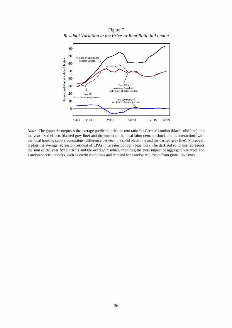
36

Figure 7

Residual Variation in the Price-to-Rent Ratio in London

Notes: The graph decomposes the average predicted price-to-rent ratio for Greater London (black solid line) into

the year fixed effects (dashed grey line) and the impact of the local labor demand shock and its interactions with

the local housing supply constraints (difference between the solid black line and the dashed grey line). Moreover,

it plots the average regression residual of LPAs in Greater London (blue line). The dark red solid line represents

the sum of the year fixed effects and the average residual, capturing the total impact of aggregate variables and

London-specific shocks, such as credit conditions and demand for London real estate from global investors.

37

Appendices

Appendix A: Proof of Proposition 3

The first part of proposition 3 is clear by inspection of the relevant expressions in the main text.

For part (ii), consider the ratio of expected long-run rents to the short-run rent, 𝑄 ≔𝑅2

𝑅1 and take

the derivative w.r.t. 𝛽:

𝜕𝑄

𝜕𝛽=

𝜙𝛿 (𝑅0 +(1 +𝛾)

1 +𝜙𝛽)

(1 +𝜙𝛽𝛿)2 (𝑅0 +1 +𝜙𝛽𝛿

)2 − (

𝜙 (1 +𝛾)

(1 +𝜙𝛽)2 (𝑅0 +1 + 𝜙𝛽𝛿

)).

This expression is smaller than zero at 𝛿 = 0. Moreover, it is continuous in 𝛿, which implies

that there exists a 𝛿̅ > 0 so that 𝜕𝑄

𝜕𝛽< 0 ∀𝛿 ∈ (0, 𝛿̅).

38

Appendix B: Appendix Tables

Appendix Table B1

Robustness of Baseline Results to the Selection of Instrument

(1) (2) (3) (4) (5) (6)

Excluding

greenbelt

instrument

Excluding

delay rate

instrument

Excluding

Labour votes

instrument

Only

greenbelt

instrument

Only

delay rate

instrument

Only

Labour votes

instrument

Log(labor demand shock) 36.429*** 38.278*** 48.328*** 46.009*** 55.174*** 33.821***

(11.322) (10.770) (13.402) (14.143) (18.402) (11.709)

Av. refusal rate of major residential

projects × log(labor demand shock) 65.038*** 62.086*** 48.848*** 52.034*** 39.026* 69.331***

(13.285) (8.927) (10.704) (11.122) (22.928) (14.161)

Share of developable land developed

in 1990 × log(labor demand shock) 84.418*** 81.511*** 79.825*** 80.872*** 74.630*** 89.172***

(22.250) (18.045) (17.349) (17.170) (21.323) (23.060)

Range between highest and lowest

altitude × log(labor demand shock) 25.101** 23.763*** 22.262*** 22.878*** 19.585* 27.256**

(10.324) (8.635) (8.032) (7.995) (10.039) (10.750)

Help to Buy (post-2015) × London

dummy -1.777 -1.192 -0.699 -0.938 0.408 -2.727

(4.058) (3.144) (2.990) (2.940) (3.935) (4.245)

LPA FEs Yes Yes Yes Yes Yes Yes

Year FEs Yes Yes Yes Yes Yes Yes

Obs. 7,555 7,555 7,555 7,555 7,555 7,555

Number of LPAs 344 344 344 344 344 344

Kleibergen-Paap F 7.003 13.36 17.35 23.01 5.783 10.06

Notes: Cluster-robust standard errors in parentheses. *** p<0.01, ** p<0.05, * p<0.1. Instruments include: Share of greenbelt land in 1973, change in

delay rate b/w 1994–96 & 2004–06, share of votes for Labour in 1983 General Election, and population density in 1911 (persons per km²). The

specifications use different sets of instruments for the average refusal rate, as denoted by the column headings.

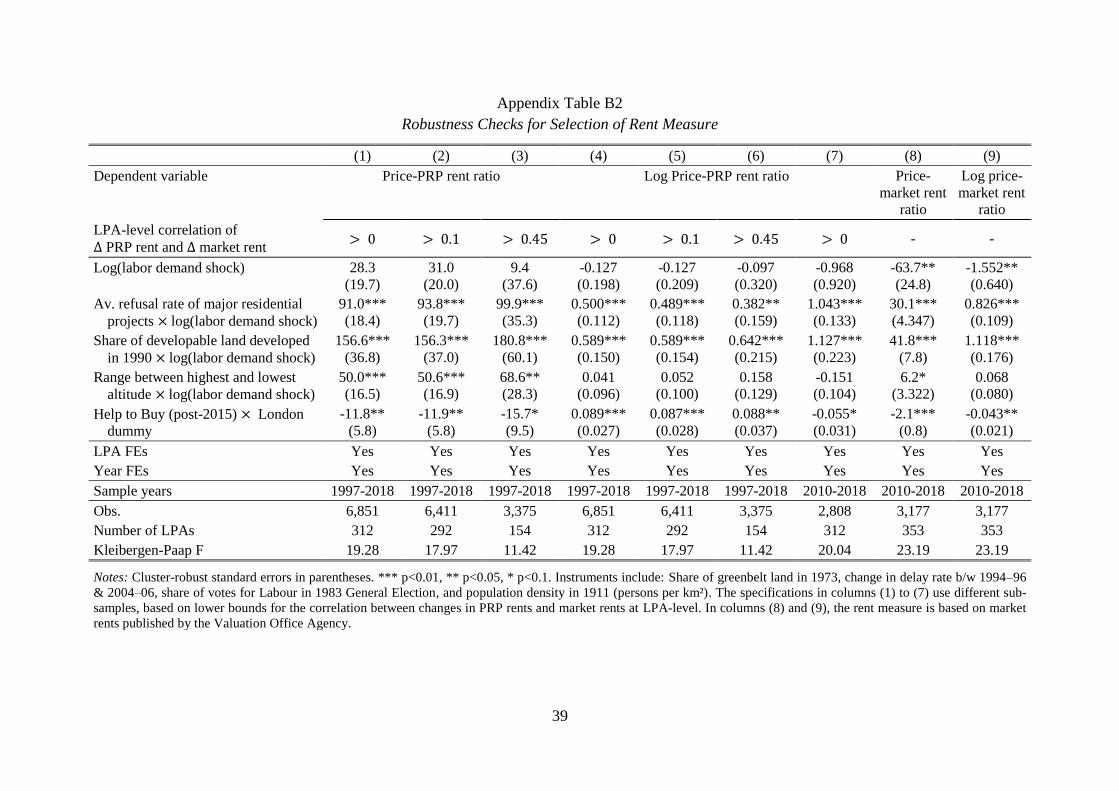
39

Appendix Table B2

Robustness Checks for Selection of Rent Measure

(1) (2) (3) (4) (5) (6) (7) (8) (9)

Dependent variable Price-PRP rent ratio Log Price-PRP rent ratio Price-

market rent

ratio

Log price-

market rent

ratio

LPA-level correlation of

Δ PRP rent and Δ market rent > 0 > 0.1 > 0.45 > 0 > 0.1 > 0.45 > 0 - -

Log(labor demand shock) 28.3 31.0 9.4 -0.127 -0.127 -0.097 -0.968 -63.7** -1.552**

(19.7) (20.0) (37.6) (0.198) (0.209) (0.320) (0.920) (24.8) (0.640)

Av. refusal rate of major residential

projects × log(labor demand shock)

91.0*** 93.8*** 99.9*** 0.500*** 0.489*** 0.382** 1.043*** 30.1*** 0.826***

(18.4) (19.7) (35.3) (0.112) (0.118) (0.159) (0.133) (4.347) (0.109)

Share of developable land developed

in 1990 × log(labor demand shock)

156.6*** 156.3*** 180.8*** 0.589*** 0.589*** 0.642*** 1.127*** 41.8*** 1.118***

(36.8) (37.0) (60.1) (0.150) (0.154) (0.215) (0.223) (7.8) (0.176)

Range between highest and lowest

altitude × log(labor demand shock)

50.0*** 50.6*** 68.6** 0.041 0.052 0.158 -0.151 6.2* 0.068

(16.5) (16.9) (28.3) (0.096) (0.100) (0.129) (0.104) (3.322) (0.080)

Help to Buy (post-2015) × London

dummy

-11.8** -11.9** -15.7* 0.089*** 0.087*** 0.088** -0.055* -2.1*** -0.043**

(5.8) (5.8) (9.5) (0.027) (0.028) (0.037) (0.031) (0.8) (0.021)

LPA FEs Yes Yes Yes Yes Yes Yes Yes Yes Yes

Year FEs Yes Yes Yes Yes Yes Yes Yes Yes Yes

Sample years 1997-2018 1997-2018 1997-2018 1997-2018 1997-2018 1997-2018 2010-2018 2010-2018 2010-2018

Obs. 6,851 6,411 3,375 6,851 6,411 3,375 2,808 3,177 3,177

Number of LPAs 312 292 154 312 292 154 312 353 353

Kleibergen-Paap F 19.28 17.97 11.42 19.28 17.97 11.42 20.04 23.19 23.19

Notes: Cluster-robust standard errors in parentheses. *** p<0.01, ** p<0.05, * p<0.1. Instruments include: Share of greenbelt land in 1973, change in delay rate b/w 1994–96

& 2004–06, share of votes for Labour in 1983 General Election, and population density in 1911 (persons per km²). The specifications in columns (1) to (7) use different sub-

samples, based on lower bounds for the correlation between changes in PRP rents and market rents at LPA-level. In columns (8) and (9), the rent measure is based on market

rents published by the Valuation Office Agency.

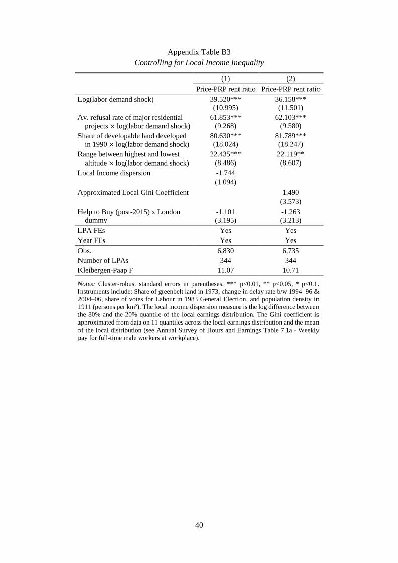
40

Appendix Table B3

Controlling for Local Income Inequality

(1) (2)

Price-PRP rent ratio Price-PRP rent ratio

Log(labor demand shock) 39.520*** 36.158***

(10.995) (11.501)

Av. refusal rate of major residential

projects × log(labor demand shock)

61.853*** 62.103***

(9.268) (9.580)

Share of developable land developed

in 1990 × log(labor demand shock)

80.630*** 81.789***

(18.024) (18.247)

Range between highest and lowest

altitude × log(labor demand shock)

22.435*** 22.119**

(8.486) (8.607)

Local Income dispersion -1.744

(1.094)

Approximated Local Gini Coefficient 1.490

(3.573)

Help to Buy (post-2015) x London

dummy

-1.101 -1.263

(3.195) (3.213)

LPA FEs Yes Yes

Year FEs Yes Yes

Obs. 6,830 6,735

Number of LPAs 344 344

Kleibergen-Paap F 11.07 10.71

Notes: Cluster-robust standard errors in parentheses. *** p<0.01, ** p<0.05, * p<0.1.

Instruments include: Share of greenbelt land in 1973, change in delay rate b/w 1994–96 &

2004–06, share of votes for Labour in 1983 General Election, and population density in

1911 (persons per km²). The local income dispersion measure is the log difference between

the 80% and the 20% quantile of the local earnings distribution. The Gini coefficient is

approximated from data on 11 quantiles across the local earnings distribution and the mean

of the local distribution (see Annual Survey of Hours and Earnings Table 7.1a - Weekly

pay for full-time male workers at workplace).

41

Appendix Table B4

Regressions in Differences

(1) (2) (3)

Δ Price-PRP rent

ratio

Δ Price-PRP rent

ratio

Δ Price-PRP rent

ratio

1-Year Diffs 3-Year Diffs 5-Year Diffs

Δ Log(labor demand shock) 49.488*** 11.579 0.470

(9.016) (18.291) (29.523)

Av. refusal rate of major residential

projects × Δ log(labor demand shock)

65.163*** 90.352*** 87.443***

(6.169) (11.514) (12.845)

Share of developable land developed in

1990 × Δ log(labor demand shock)

53.198*** 38.729*** 37.168***

(7.215) (11.056) (14.314)

Range between highest and lowest

altitude × Δ log(labor demand shock)

11.943*** 11.477* 9.409

(4.396) (6.913) (7.820)

Δ Help to Buy (post-2015) x London

dummy

0.629 0.733 0.825

(0.647) (0.798) (0.964)

LPA FEs Yes Yes Yes

Year FEs Yes Yes Yes

Obs. 7,211 6,523 5,835

Number of LPAs 344 344 344

Kleibergen-Paap F 13.33 14.51 13.81

Notes: Cluster-robust standard errors in parentheses. *** p<0.01, ** p<0.05, * p<0.1. Instruments include: Share of

greenbelt land in 1973, change in delay rate b/w 1994–96 & 2004–06, share of votes for Labour in 1983 General

Election, and population density in 1911 (persons per km²). All regressions are in differences. The column heading

indicates the number of years over which the differences are computed (1, 3, and 5 years). The regressions also include

LPA and year FEs to capture average LPA-level changes and national-level changes over the respective period.

42

Appendix Table B5

Relative Attractiveness of Homeownership

(1) (2) (3) (4)

Adjusted

LDS

Real Mortg.

Interest Rate Mortgage

Rate Spread

Help to Buy

Log(labor demand shock) 39.374*** 30.192** 30.032** 40.067***

(10.617) (12.581) (12.514) (9.942)

Av. refusal rate of major residential projects × log(labor demand shock)

59.973*** 51.646*** 61.115*** 51.856***

(8.786) (7.048) (8.376) (7.930)

Share of developable land developed in 1990 × log(labor demand shock)

79.100*** 68.621*** 85.019*** 47.401***

(17.890) (14.251) (16.569) (11.840)

Range between highest and lowest altitude × log(labor demand shock)

22.675*** 18.337*** 21.447*** 31.935***

(8.509) (7.033) (8.056) (7.597)

Help to Buy (post-2015) x London dummy -0.790 -0.069 -2.080 -1.498

(3.129) (2.903) (2.916) (2.884)

Av. refusal rate of major residential projects ×

Real Mortgage Interest Rate

-0.525***

(0.141)

Share of developable land developed in 1990 × Real Mortgage Interest Rate

-0.506***

(0.192)

Range between highest and lowest altitude × Real Mortgage Interest Rate

-0.226**

(0.090)

Av. refusal rate of major residential projects ×

Mortgage Interest Rate Spread

-0.600

(0.401)

Share of developable land developed in 1990 × Mortgage Interest Rate Spread

0.911*

(0.474)

Range between highest and lowest altitude × Mortgage Interest Rate Spread

-0.839***

(0.289)

Av. refusal rate of major residential projects ×

Help to Buy (post-2012)

1.010

(0.635)

Share of developable land developed in 1990 × Help to Buy (post-2012)

4.344***

(0.900)

Range between highest and lowest altitude × Help to Buy (post-2012)

-1.148**

(0.485)

LPA FEs Yes Yes Yes Yes

Year FEs Yes Yes Yes Yes

Obs. 7,555 7,555 7,555 7,555

Number of LPAs 344 344 344 344

Kleibergen-Paap F 9.733 5.180 5.225 7.167

Notes: Cluster-robust standard errors in parentheses. *** p<0.01, ** p<0.05, * p<0.1. Instruments include: Share of

greenbelt land in 1973, change in delay rate b/w 1994–96 & 2004–06, share of votes for Labour in 1983 General Election,

and population density in 1911 (persons per km²). In model (1), the labor demand shock is adjusted by excluding variation

due to the banking and real estate service sectors (SIC 2007 classifications K, L) from the national-level time series for

the service and distribution sector. The interactions of the supply constraints with the real mortgage interest rate (model

(2)), the spread (mortgage rate minus sight deposit rate) (model (3)) and of the Post-2012 dummy (model (4)) are

instrumented by the interactions of the respective variable with the instruments discussed in Section 3.2.

43

Appendix C: Appendix Figures

Figure C1

Distribution of the Correlation between Changes in Market Rents and PRP Rents at LPA-

Level

Notes: The graph displays the distribution of the correlation between changes in market rents and PRP rents at

LPA-level. The dashed vertical lines indicate the three thresholds used to select the samples for Table B2 in

Appendix B (correlation exceeding 0.0, 0.1, and 0.45).

44

Figure C2

Placebo Test: Simulated Densities for the Baseline Regression Coefficients

Panel A. Log LDS independent effect Panel B. Log LDS × avg. refusal rate

Panel C. Log LDS × share developed Panel D. Log LDS × elevation range

Notes: All four graphs are based on the model displayed in column (5) of Table 2. The graphs display the

coefficient distributions from 2,000 simulated placebo shocks, which are used instead of the shift-share labor

demand shock. The red vertical bars indicate the locations of the baseline coefficient estimates.

45

Online Appendix – Not for Publication

Online Appendix O-A: Detailed Data Description

This online appendix provides details on the various sources and computation of variables used

in our empirical analysis.

House prices. We extend and refine the house price panel of Hilber and Vermeulen (2016)

from 2008 to 2018. We use the same composition adjustment to calculate average nominal

house prices by LPA and year from the Price Paid Data of the UK Land Registry. The Price

Paid Data contain all property sales in England of properties sold for full market value. The

1974-1994 panel is based on transactions recorded in the Survey of Mortgage Lenders. We

drop transactions made under the Right-to-Buy scheme. The scheme allowed tenants in council

housing to buy their housing units at a substantial discount. We append the full period for which

the Price Paid Data are available, 1995-2018, to the adjusted 1974-1994 panel from Hilber and

Vermeulen (2016). We deflate the nominal index by the RPIX.

Labor demand shock. We follow the methodology from Hilber and Vermeulen (2016).

Specifically, we use industry shares at LPA-level from 1971 and Standard Industrial

Classification (SIC) weights. We use seven broad industries.

The 1971 industry shares come from the Census of Population 1971. Like Hilber and

Vermeulen (2016), we combine two national time series of employment growth by industry in

order to arrive at a time series that covers the whole period, 1971 to 2018. The Census of

Employment – Employee Analysis disaggregates employment of male fulltime employees in

England into three-digit 1968 SIC categories. It is available from 1971 to 1978. Table O-A1

shows the disaggregation of employment for 1971 at the national level, for the Census of

Employment and the Census of Population. Differences are attributable to the fact that unlike

the Census of Population, the Census of Employment excludes women, part-time workers, and

the self-employed.

Table O-A1

Industry Composition of Employment in 1971

% of total employment in 1971

Industry, as described in Census England

(Census)

Great Britain

(Employer Survey)

Agriculture 2% 2%

Mining 1% 3%

Manufacturing 35% 43%

Construction 7% 8%

Utilities; Transport 8% 12%

Distribution & Services 39% 24%

National & Local Government Service & Defence 7% 7%

Total 100% 100% Source: Hilber and Vermeulen (2016).

For the period from 1978 until 2018, we use the Workforce Jobs by Industry data of

employment by all fulltime workers in the UK, disaggregated to broad industries (one digit

46

2007 SIC). The Office of National Statistics provides these data, drawing on employment and

labor force surveys. Consistent with the 1971 Census of Population, this data includes the self-

employed and women, but it excludes part-time workers.

The time series have one overlapping year, which allows us to calculate internally consistent

growth rates. We use them to form industry-level employment indices for England as a whole,

where 1971 is the base year. We then use the development of an industry’s employment at the

national level to extrapolate local employment in that industry in a given year, by simply

multiplying the index value in that year with the industry’s employment in the LPA in 1971.

Our productivity shock measure is the sum over the extrapolated employment in all seven

industries.

Share of greenbelt land in 1973. One of our instruments for the average refusal rate is the share

of greenbelt land in 1973. In order to construct the variable, we digitized a map of recreational

land in Great Britain (Lawrence 1973). The map provides information on greenbelts designated

prior to 1973. We match the map with LPA delineations of 2001 and use geographic

information software to calculate the share of designated greenbelt land in each LPA in 1973.

Market rents, 2010—2018. The rents data are taken from the “Private Rental Market Statistics”

provided by the Valuation Office Agency. The Valuation Office Agency conducts surveys to

collect data on rents. The Valuation Office Agency publishes average rents separately for

different dwelling unit types (by number of rooms) for periods of 12 months (bi-annually, in

March and October). We use the March publication and assign it to the same year. As an

example, the March 2015 publication covers March 2015—February 2016 and it was assigned

to the year 2015 in the panel. We follow the same aggregation strategy as for the house price

index. We first calculate the average share of each dwelling unit type by LPA and use these

shares as aggregation weights in the second step. The nominal average rent by LPA and year

is the weighted sum of mean rents reported for each category in that LPA and year. We deflate

the nominal rents by the RPIX.

Private Registered Provider rents, 1997—2018. The uk.gov Table 704 of the UK Housing

Statistics reports mean rents charged by Private Registered Providers (PRP), by year (1997—

2018), and LPA. The statistic only includes larger PRPs with more than 1,000 beds, and refers

to self-contained units. Typically, PRP are profit-maximizing organizations. However, PRP

rents are subject to a rent ceiling that is pegged to the current market rent. We deflate the

nominal rents by the RPIX. For more details on the definition of the rent ceiling, see the

Guidance on Rents for Social Housing, Department for Communities and Local Government

(now: Ministry of Housing, Communities and Local Government), May 2014,

https://www.gov.uk/government/publications/

guidance-on-rents-for-social-housing.

47

Online Appendix O-B: Additional Tables

Table O-B1

Specifications separate for Periods with Positive and Negative Labor Demand Shocks –

Results for Log Real House Prices and Log Real Rents

(1) (2) (3) (4)

Prices 2SLS a)

1997-2018 b), c)

Prices 2SLS a)

1997-2018 b), c)

Rents 2SLS a)

1997-2018 c)

Rents 2SLS a)

1997-2018 c)

LDS>0 LDS≤0 LDS>0 LDS≤0

Log(labor demand shock) -0.002 -0.467 -0.050 0.059

(0.186) (0.329) (0.145) (0.190)

Av. refusal rate × log(labor demand shock)

0.860***

(0.136)

0.077

(0.305)

0.308***

(0.078)

0.032

(0.287)

Share developed × log(labor demand shock)

1.183*** -0.668* 0.534*** -0.176

(0.274) (0.361) (0.090) (0.140)

Altitude range × log(labor demand shock)

0.237* -0.241*** 0.145** -0.097*

(0.135) (0.075) (0.061) (0.058)

Help to Buy (post-2015) × London dummy

0.022 -0.051***

(0.049) (0.016)

LPA FEs Yes Yes Yes Yes

Year FEs Yes Yes Yes Yes

Obs. 6,304 1,248 6,304 1,248

Number of LPAs 344 341 344 341

Kleibergen-Paap F 9.188 6.985 9.188 6.985

Notes: Cluster-robust standard errors in parentheses. *** p<0.01, ** p<0.05, * p<0.1. a) First stage

results are reported in Table 3 in the main text. Instruments include: Share of greenbelt land in 1973,

change in delay rate b/w 1994–96 & 2004–06, share of votes for Labour in 1983 General Election,

and population density in 1911 (persons per km²). b) Observations with missing rental data removed

to make price and rent specifications comparable. c) PRP vs. market rent outliers (mean log market

rent > 7.5, based on Figure 4) removed.

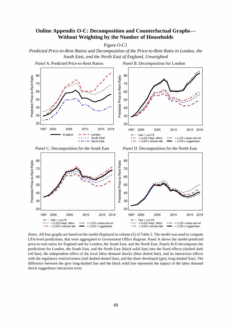
48

Online Appendix O-C: Decomposition and Counterfactual Graphs—

Without Weighting by the Number of Households

Figure O-C1

Predicted Price-to-Rent Ratios and Decomposition of the Price-to-Rent Ratio in London, the

South East, and the North East of England, Unweighted

Panel A. Predicted Price-to-Rent Ratios Panel B. Decomposition for London

Panel C. Decomposition for the South East Panel D. Decomposition for the North East

Notes: All four graphs are based on the model displayed in column (5) of Table 2. The model was used to compute

LPA-level predictions, that were aggregated to Government Office Regions. Panel A shows the model-predicted

price-to-rent ratios for England and for London, the South East, and the North East. Panels B-D decomposes the

predictions for London, the South East, and the North East (black solid line) into the fixed effects (dashed dark

red line), the independent effect of the local labor demand shocks (blue dotted line), and its interaction effects

with the regulatory restrictiveness (red dashed-dotted line), and the share developed (grey long-dashed line). The

difference between the grey long-dashed line and the black solid line represents the impact of the labor demand

shock-ruggedness interaction term.

49

Figure O-C2

Counterfactual Decomposition Relative to a Location with Supply Constraints at the 10%

Sample Quantiles, Unweighted

Panel A. Average Supply Constraints Panel B. London’s Supply Constraints

Panel C. The South East’s Supply Constraints Panel D. The North East’s Supply

Constraints

Notes: All four graphs are based on the model displayed in column (5) of Table 2. The model was used to compute

LPA-level predictions for a standardized labor demand shock. The predictions were aggregated to Government

Office Regions. Panels A-D shows model-predicted price-to-rent ratios for (household-weighted) average supply

constraints in England, London, the South East, and the North East (black solid lines) and for a location where all

supply constraints are set to the respective 10% sample quantile (dark red dashed lines), shifted vertically to match

the 1997 price-to-rent ratio of the location. The red dashed-dotted lines represents the impact of changing the

refusal from the 10% quantile to the counterfactual location’s refusal rate. The dashed grey line adds the impact

of changing the share developed from the 10% quantile to the respective location’s share developed. The

remaining difference to the black solid line represents the impact of changing the elevation range from the 10%

quantile to the respective location’s elevation range.

CENTRE FOR ECONOMIC PERFORMANCE Recent Discussion Papers

1742 Swati Dhingra

Rebecca Freeman Hanwei Huang

The impacts of non-tariff barriers on trade and welfare

1741 Josh De Lyon João Paulo Pessoa

Worker and firm responses to trade shocks: The UK-China case

1740 Carlo Altomonte Domenico Favoino Monica Morlacco Tommaso Sonno

Markups, intangible capital and heterogeneous financial frictions

1739 Chad Bown Paola Conconi Aksel Erbahar Lorenzo Trimarchi

Trade protection along supply chains

1738 Christian Krekel Julia Rechlitz Johannes Rode Alexander Zerrahn

Quantifying the externalities of renewable energy plants using wellbeing data: The case of biogas

1737 Nick Jacob Giordano Mion

The UK’s great demand and supply recession

1736 Gabriel M. Ahlfeldt Fabian Bald Duncan Roth Tobias Seidel

Quality of life in a dynamic spatial model

1735 Kilian Huber Are bigger banks better? Firm-level evidence from Germany

1734 César Ducruet Réka Juhász Dávid Krisztián Nagy Claudia Steinwender

All aboard: the effects of port development

1733 Jonathan Colmer John Voorheis

The grandkids aren’t alright: the intergenerational effects of prenatal pollution exposure

1732 Kabir Dasgupta André Diegmann Tom Kirchmaier Alexander Plum

Heterogeneity in criminal behavior after child birth: the role of ethnicity

1731 Andreas Diemer Tanner Regan

No inventor is an island: social connectedness and the geography of knowledge flows in the US

1730 Hanming Fang Chunmian Ge Hanwei Huang Hongbin Li

Pandemics, global supply chains, and local labor demand: evidence from 100 million posted jobs in China

1729 Ria Ivandić Tom Kirchmaier Ben Linton

Changing patterns of domestic abuse during COVID-19 lockdown

1728 Jonathan Colmer Ralf Martin Mirabelle Muûls Ulrich J. Wagner

Does pricing carbon mitigate climate change? Firm-level evidence from the European Union emissions trading scheme

1727 Tony Beatton Michael P. Kidd Matteo Sandi

School indiscipline and crime

1726 Maximilian v. Ehrlich Henry G. Overman

Place-based policies and spatial disparities across European cities

1725 Gabriel M. Ahlfeldt Thilo N. H. Albers Kristian Behrens

Prime Locations

The Centre for Economic Performance Publications Unit Tel: +44 (0)20 7955 7673 Email info@cep.lse.ac.uk Website: http://cep.lse.ac.uk Twitter: @CEP_LSE