Why estimate visual motion? - courses.cs.washington.edu...Why estimate visual motion? Visual Motion...
22
Motion estimation Computer Vision CSE576, Spring 2005 Richard Szeliski CSE 576, Spring 2005 Motion estimation 2 Why estimate visual motion? Visual Motion can be annoying • Camera instabilities, jitter • Measure it; remove it (stabilize) Visual Motion indicates dynamics in the scene • Moving objects, behavior • Track objects and analyze trajectories Visual Motion reveals spatial layout • Motion parallax CSE 576, Spring 2005 Motion estimation 3 Today’s lecture Motion estimation • image warping (skip: see handout) • patch-based motion (optic flow) • parametric (global) motion • application: image morphing • advanced: layered motion models CSE 576, Spring 2005 Motion estimation 4 Readings • Bergen et al. Hierarchical model-based motion estimation. ECCV’92, pp. 237–252. • Szeliski, R. Image Alignment and Stitching: A Tutorial, MSR-TR-2004-92, Sec. 3.4 & 3.5. • Shi, J. and Tomasi, C. (1994). Good features to track. In CVPR’94, pp. 593–600. • Baker, S. and Matthews, I. (2004). Lucas- kanade 20 years on: A unifying framework. IJCV, 56(3), 221–255.
Transcript of Why estimate visual motion? - courses.cs.washington.edu...Why estimate visual motion? Visual Motion...
1
Motion estimation
Computer VisionCSE576, Spring 2005
Richard Szeliski
CSE 576, Spring 2005 Motion estimation 2
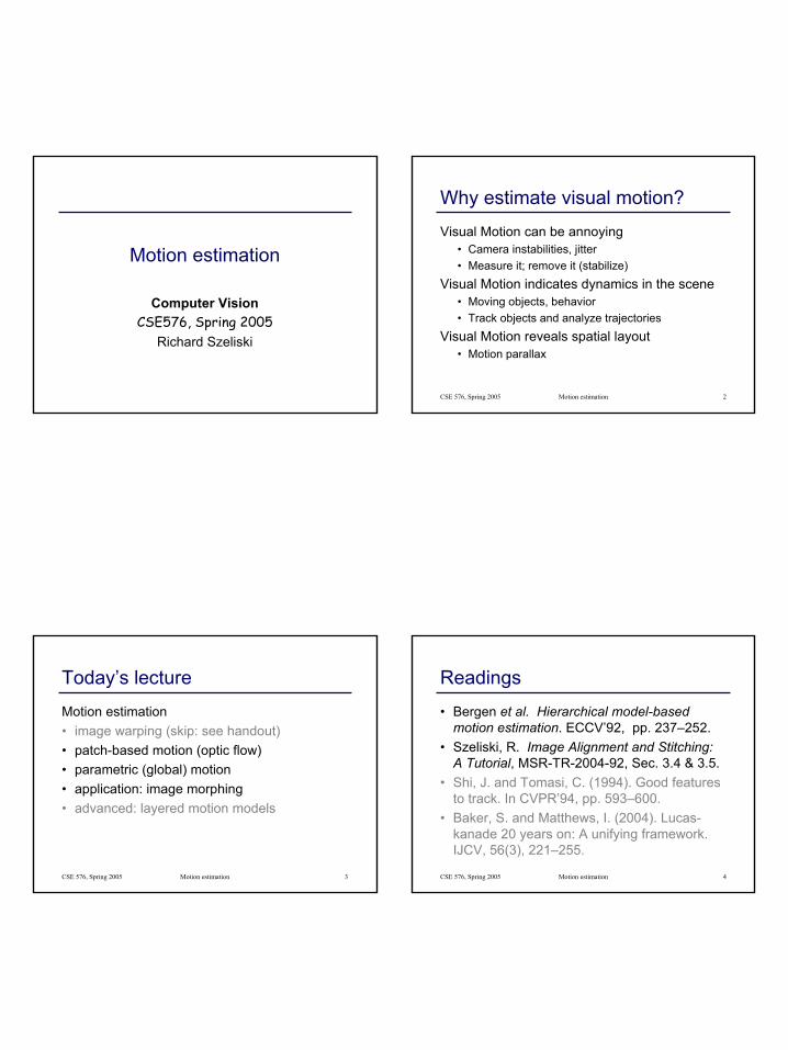
Why estimate visual motion?
Visual Motion can be annoying• Camera instabilities, jitter• Measure it; remove it (stabilize)
Visual Motion indicates dynamics in the scene• Moving objects, behavior• Track objects and analyze trajectories
Visual Motion reveals spatial layout • Motion parallax
CSE 576, Spring 2005 Motion estimation 3
Today’s lecture
Motion estimation• image warping (skip: see handout)• patch-based motion (optic flow)• parametric (global) motion• application: image morphing• advanced: layered motion models
CSE 576, Spring 2005 Motion estimation 4
Readings
• Bergen et al. Hierarchical model-based motion estimation. ECCV’92, pp. 237–252.
• Szeliski, R. Image Alignment and Stitching: A Tutorial, MSR-TR-2004-92, Sec. 3.4 & 3.5.
• Shi, J. and Tomasi, C. (1994). Good features to track. In CVPR’94, pp. 593–600.
• Baker, S. and Matthews, I. (2004). Lucas-kanade 20 years on: A unifying framework. IJCV, 56(3), 221–255.
2
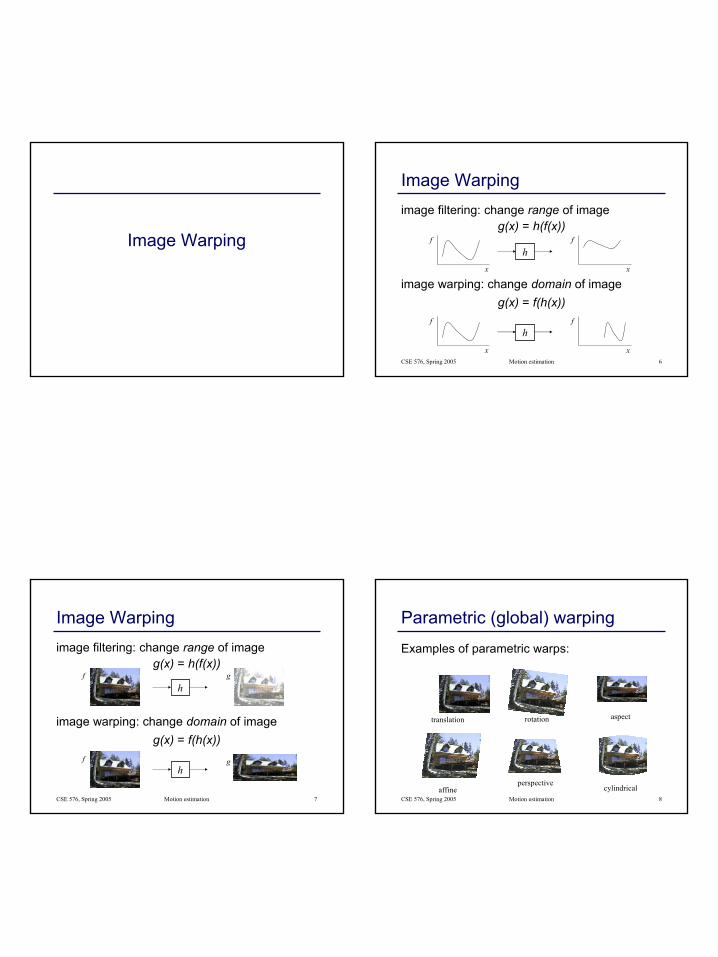
Image Warping
CSE 576, Spring 2005 Motion estimation 6
Image Warpingimage filtering: change range of image
g(x) = h(f(x))
image warping: change domain of imageg(x) = f(h(x))
f
x
hf
x
f
x
hf
x
CSE 576, Spring 2005 Motion estimation 7
Image Warpingimage filtering: change range of image
g(x) = h(f(x))
image warping: change domain of imageg(x) = f(h(x))
h
h
f
f g
g
CSE 576, Spring 2005 Motion estimation 8
Parametric (global) warping
Examples of parametric warps:
translation rotation aspect
affineperspective
cylindrical
3
CSE 576, Spring 2005 Motion estimation 9
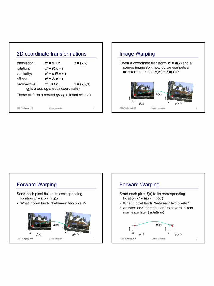
2D coordinate transformations
translation: x’ = x + t x = (x,y)rotation: x’ = R x + tsimilarity: x’ = s R x + taffine: x’ = A x + tperspective: x’ ≅ H x x = (x,y,1)
(x is a homogeneous coordinate)
These all form a nested group (closed w/ inv.)
CSE 576, Spring 2005 Motion estimation 10
Image Warping
Given a coordinate transform x’ = h(x) and a source image f(x), how do we compute a transformed image g(x’) = f(h(x))?
f(x) g(x’)x x’
h(x)
CSE 576, Spring 2005 Motion estimation 11
Forward Warping
Send each pixel f(x) to its corresponding location x’ = h(x) in g(x’)
f(x) g(x’)x x’
h(x)
• What if pixel lands “between” two pixels?
CSE 576, Spring 2005 Motion estimation 12
Forward Warping
Send each pixel f(x) to its corresponding location x’ = h(x) in g(x’)
f(x) g(x’)x x’
h(x)
• What if pixel lands “between” two pixels?• Answer: add “contribution” to several pixels,
normalize later (splatting)
4
CSE 576, Spring 2005 Motion estimation 13
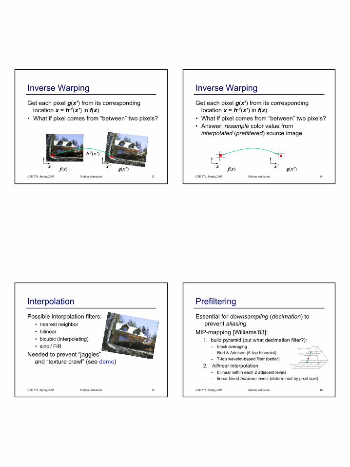
Inverse Warping
Get each pixel g(x’) from its corresponding location x = h-1(x’) in f(x)
f(x) g(x’)x x’
h-1(x’)
• What if pixel comes from “between” two pixels?
CSE 576, Spring 2005 Motion estimation 14
Inverse Warping
Get each pixel g(x’) from its corresponding location x = h-1(x’) in f(x)
• What if pixel comes from “between” two pixels?• Answer: resample color value from
interpolated (prefiltered) source image
f(x) g(x’)x x’
CSE 576, Spring 2005 Motion estimation 15
Interpolation
Possible interpolation filters:• nearest neighbor• bilinear• bicubic (interpolating)• sinc / FIR
Needed to prevent “jaggies”and “texture crawl” (see demo)
CSE 576, Spring 2005 Motion estimation 16
Prefiltering
Essential for downsampling (decimation) to prevent aliasing
MIP-mapping [Williams’83]:1. build pyramid (but what decimation filter?):
– block averaging– Burt & Adelson (5-tap binomial)– 7-tap wavelet-based filter (better)
2. trilinear interpolation– bilinear within each 2 adjacent levels– linear blend between levels (determined by pixel size)
5
CSE 576, Spring 2005 Motion estimation 17
Prefiltering
Essential for downsampling (decimation) to prevent aliasing
Other possibilities:• summed area tables• elliptically weighted Gaussians (EWA)
[Heckbert’86]
Patch-based motion estimation
CSE 576, Spring 2005 Motion estimation 19
Classes of Techniques
Feature-based methods• Extract visual features (corners, textured areas) and track them
over multiple frames• Sparse motion fields, but possibly robust tracking• Suitable especially when image motion is large (10-s of pixels)
Direct-methods• Directly recover image motion from spatio-temporal image
brightness variations• Global motion parameters directly recovered without an
intermediate feature motion calculation• Dense motion fields, but more sensitive to appearance variations• Suitable for video and when image motion is small (< 10 pixels)
CSE 576, Spring 2005 Motion estimation 20
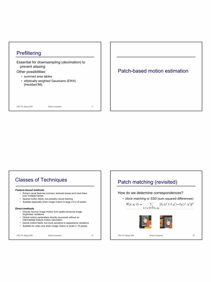
Patch matching (revisited)
How do we determine correspondences?• block matching or SSD (sum squared differences)
6
CSE 576, Spring 2005 Motion estimation 21
Brightness Constancy Equation:
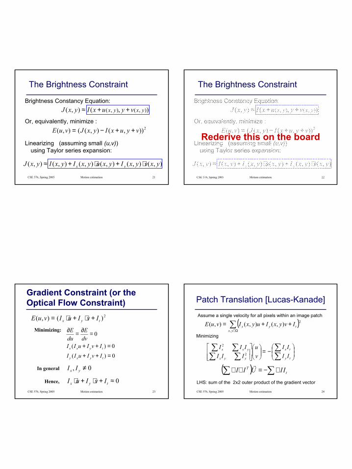
The Brightness Constraint
),(),( ),(),( yxyx vyuxIyxJ ++≈
Or, equivalently, minimize :2)),(),((),( vyuxIyxJvuE ++−=
),(),(),(),(),(),( yxvyxIyxuyxIyxIyxJ yx ⋅+⋅+≈
Linearizing (assuming small (u,v))using Taylor series expansion:
CSE 576, Spring 2005 Motion estimation 22
Brightness Constancy Equation:
The Brightness Constraint
),(),( ),(),( yxyx vyuxIyxJ ++≈
Or, equivalently, minimize :2)),(),((),( vyuxIyxJvuE ++−=
),(),(),(),(),(),( yxvyxIyxuyxIyxIyxJ yx ⋅+⋅+≈
Linearizing (assuming small (u,v))using Taylor series expansion:
Rederive this on the board
CSE 576, Spring 2005 Motion estimation 23
Gradient Constraint (or the Optical Flow Constraint)
2)(),( tyx IvIuIvuE +⋅+⋅=
Minimizing:
0)(
0)(
0
=++
=++
=∂=∂
tyxy
tyxx
IvIuII
IvIuIIdvE
duE
In general 0, ≠yx II
0≈+⋅+⋅ tyx IvIuIHence,
CSE 576, Spring 2005 Motion estimation 24
Patch Translation [Lucas-Kanade]
( )∑Ω∈
++=yx
tyx IvyxIuyxIvuE,
2),(),(),(
Minimizing
Assume a single velocity for all pixels within an image patch
−=
∑∑
∑∑∑∑
ty
tx
yyx
yxx
IIII
vu
IIIIII2
2
( ) tT IIUII ∑∑ ∇−=∇∇r
LHS: sum of the 2x2 outer product of the gradient vector
7
CSE 576, Spring 2005 Motion estimation 25
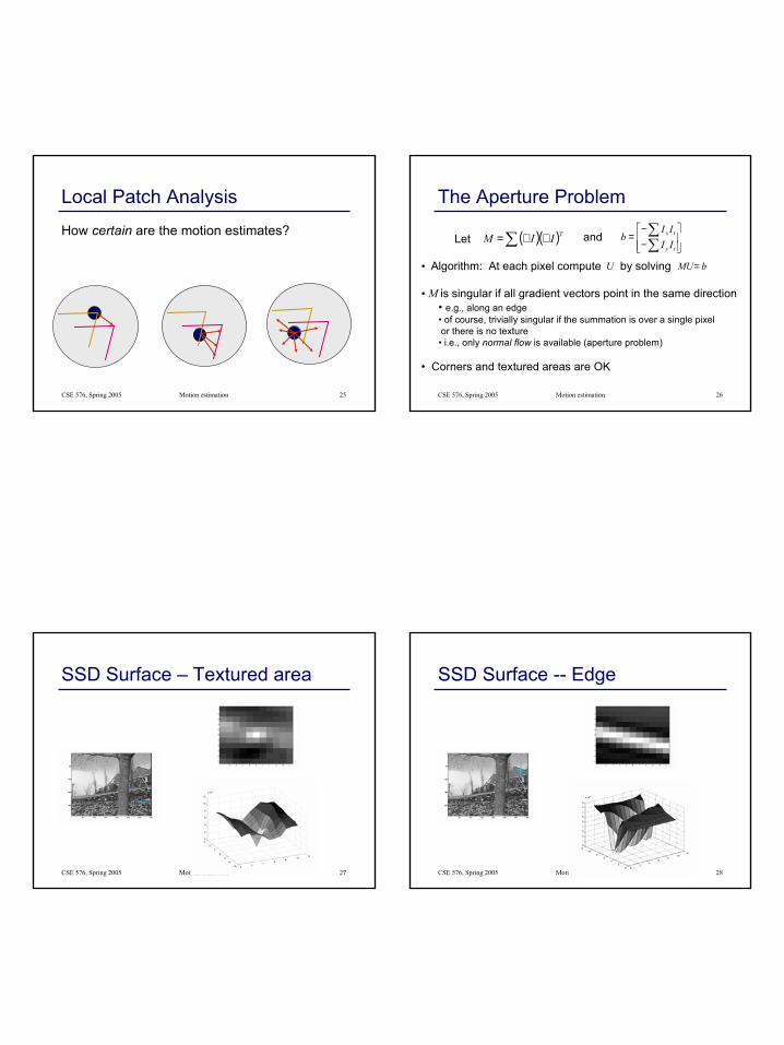
Local Patch Analysis
How certain are the motion estimates?
CSE 576, Spring 2005 Motion estimation 26
The Aperture Problem
( )( )∑ ∇∇= TIIMLet
• Algorithm: At each pixel compute by solving
• M is singular if all gradient vectors point in the same direction• e.g., along an edge• of course, trivially singular if the summation is over a single pixelor there is no texture• i.e., only normal flow is available (aperture problem)
• Corners and textured areas are OK
and
−−
=∑∑
ty
tx
IIII
b
U bMU=
CSE 576, Spring 2005 Motion estimation 27
SSD Surface – Textured area
CSE 576, Spring 2005 Motion estimation 28
SSD Surface -- Edge
8
CSE 576, Spring 2005 Motion estimation 29
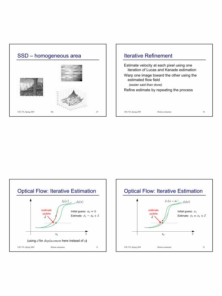
SSD – homogeneous area
CSE 576, Spring 2005 Motion estimation 30
Iterative Refinement
Estimate velocity at each pixel using one iteration of Lucas and Kanade estimation
Warp one image toward the other using the estimated flow field(easier said than done)
Refine estimate by repeating the process
CSE 576, Spring 2005 Motion estimation 31
Optical Flow: Iterative Estimation
xx0
Initial guess: Estimate:
estimate update
(using d for displacement here instead of u)
CSE 576, Spring 2005 Motion estimation 32
Optical Flow: Iterative Estimation
xx0
estimate update
Initial guess: Estimate:
9
CSE 576, Spring 2005 Motion estimation 33
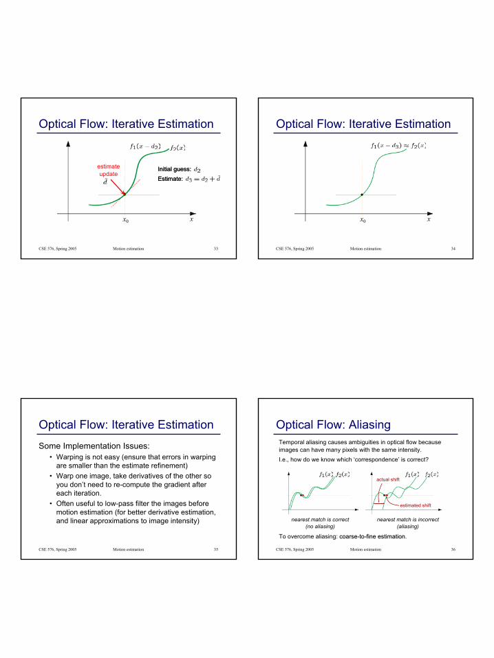
Optical Flow: Iterative Estimation
xx0
Initial guess: Estimate:Initial guess: Estimate:
estimate update
CSE 576, Spring 2005 Motion estimation 34
Optical Flow: Iterative Estimation
xx0
CSE 576, Spring 2005 Motion estimation 35
Optical Flow: Iterative Estimation
Some Implementation Issues:• Warping is not easy (ensure that errors in warping
are smaller than the estimate refinement)• Warp one image, take derivatives of the other so
you don’t need to re-compute the gradient after each iteration.
• Often useful to low-pass filter the images before motion estimation (for better derivative estimation, and linear approximations to image intensity)
CSE 576, Spring 2005 Motion estimation 36
Optical Flow: AliasingTemporal aliasing causes ambiguities in optical flow because images can have many pixels with the same intensity.I.e., how do we know which ‘correspondence’ is correct?
nearest match is correct (no aliasing)
nearest match is incorrect (aliasing)
To overcome aliasing: coarsecoarse--toto--fine estimationfine estimation.
actual shift
estimated shift
10
CSE 576, Spring 2005 Motion estimation 37
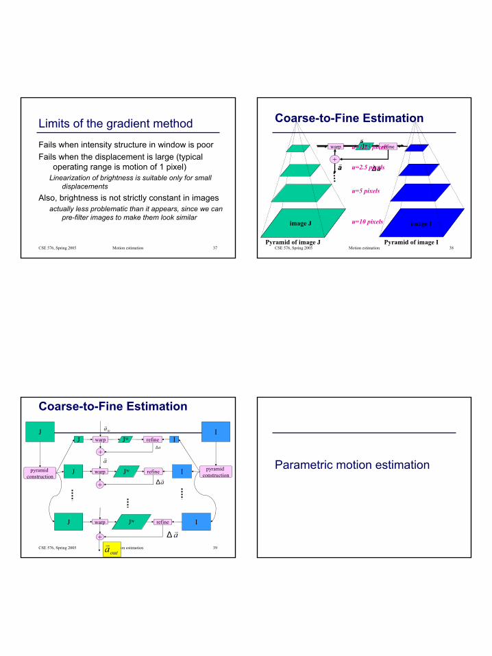
Limits of the gradient method
Fails when intensity structure in window is poorFails when the displacement is large (typical
operating range is motion of 1 pixel)Linearization of brightness is suitable only for small
displacementsAlso, brightness is not strictly constant in images
actually less problematic than it appears, since we can pre-filter images to make them look similar
CSE 576, Spring 2005 Motion estimation 38
image Iimage J
avJwwarp refine
av
a∆v
+
Pyramid of image J Pyramid of image I
image Iimage J
Coarse-to-Fine Estimation
u=10 pixels
u=5 pixels
u=2.5 pixels
u=1.25 pixels
CSE 576, Spring 2005 Motion estimation 39
J Jw Iwarp refine
inav
av∆+
J Jw Iwarp refine
av
av∆+
J
pyramid construction
J Jw Iwarp refine
av∆+
I
pyramid construction
outav
Coarse-to-Fine Estimation
Parametric motion estimation
11
CSE 576, Spring 2005 Motion estimation 41
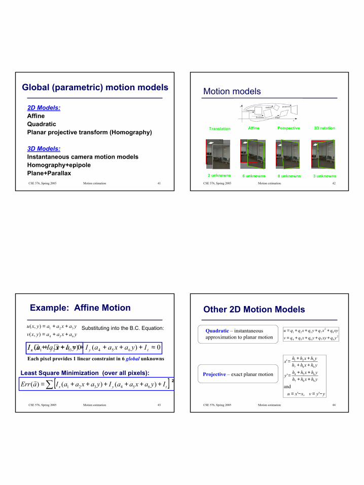
Global (parametric) motion models
2D Models:AffineQuadraticPlanar projective transform (Homography)
3D Models:Instantaneous camera motion models Homography+epipolePlane+Parallax
CSE 576, Spring 2005 Motion estimation 42
Motion models
Translation
2 unknowns
Affine
6 unknowns
Perspective
8 unknowns
3D rotation
3 unknowns
CSE 576, Spring 2005 Motion estimation 43
0)()( 654321 ≈++++++ tyx IyaxaaIyaxaaI
Example: Affine Motion
Substituting into the B.C. Equation:yaxaayxvyaxaayxu
654
321
),(),(
++=++=
Each pixel provides 1 linear constraint in 6 global unknowns
0≈+⋅+⋅ tyx IvIuI
[ ] 2∑ ++++++= tyx IyaxaaIyaxaaIaErr )()()( 654321r
Least Square Minimization (over all pixels):
CSE 576, Spring 2005 Motion estimation 44
Quadratic – instantaneous approximation to planar motion
Other 2D Motion Models
287654
82
7321
yqxyqyqxqqv
xyqxqyqxqqu
++++=
++++=
yyvxxu
yhxhhyhxhhy
yhxhhyhxhhx
−=−=
++++=
++++=
',' and
'
'
987
654
987
321
Projective – exact planar motion
12
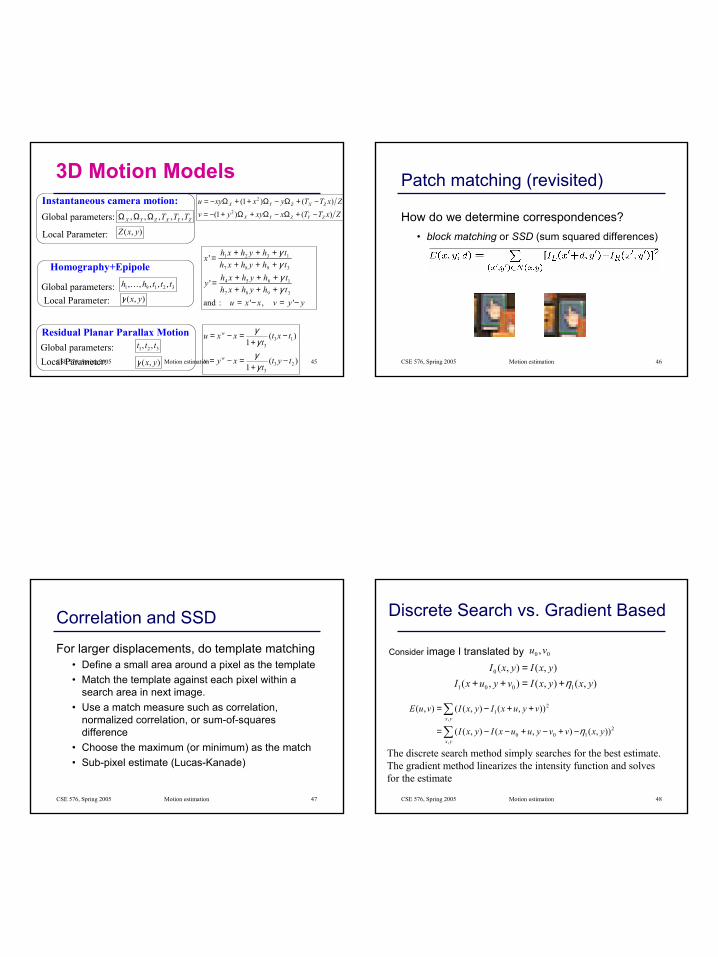
CSE 576, Spring 2005 Motion estimation 45
3D Motion Models
ZxTTxxyyv
ZxTTyxxyu
ZYZYX
ZXZYX
)()1(
)()1(2
2
−+Ω−Ω+Ω+−=
−+Ω−Ω++Ω−=
yyvxxuthyhxhthyhxhy
thyhxhthyhxhx
−=−=++++++=
++++++=
',' :and
'
'
3987
1654
3987
1321
γγγγ
)(1
)(1
233
133
tytt
xyv
txtt
xxu
w
w
−+
=−=
−+
=−=
γγγγ
Local Parameter:
ZYXZYX TTT ,,,,, ΩΩΩ
),( yxZ
Instantaneous camera motion:Global parameters:
Global parameters: 32191 ,,,,, ttthh K
),( yxγ
Homography+Epipole
Local Parameter:
Residual Planar Parallax MotionGlobal parameters: 321 ,, ttt
),( yxγLocal Parameter: CSE 576, Spring 2005 Motion estimation 46
Patch matching (revisited)
How do we determine correspondences?• block matching or SSD (sum squared differences)
CSE 576, Spring 2005 Motion estimation 47
Correlation and SSD
For larger displacements, do template matching• Define a small area around a pixel as the template• Match the template against each pixel within a
search area in next image.• Use a match measure such as correlation,
normalized correlation, or sum-of-squares difference
• Choose the maximum (or minimum) as the match• Sub-pixel estimate (Lucas-Kanade)
CSE 576, Spring 2005 Motion estimation 48
Discrete Search vs. Gradient Based
Consider image I translated by
21
,00
2
,1
)),(),(),((
)),(),((),(
yxvvyuuxIyxI
vyuxIyxIvuE
yx
yx
η−+−+−−=
++−=
∑
∑
00 ,vu
),(),(),(),(),(
1001
0
yxyxIvyuxIyxIyxI
η+=++=
The discrete search method simply searches for the best estimate.The gradient method linearizes the intensity function and solves for the estimate
13
CSE 576, Spring 2005 Motion estimation 49
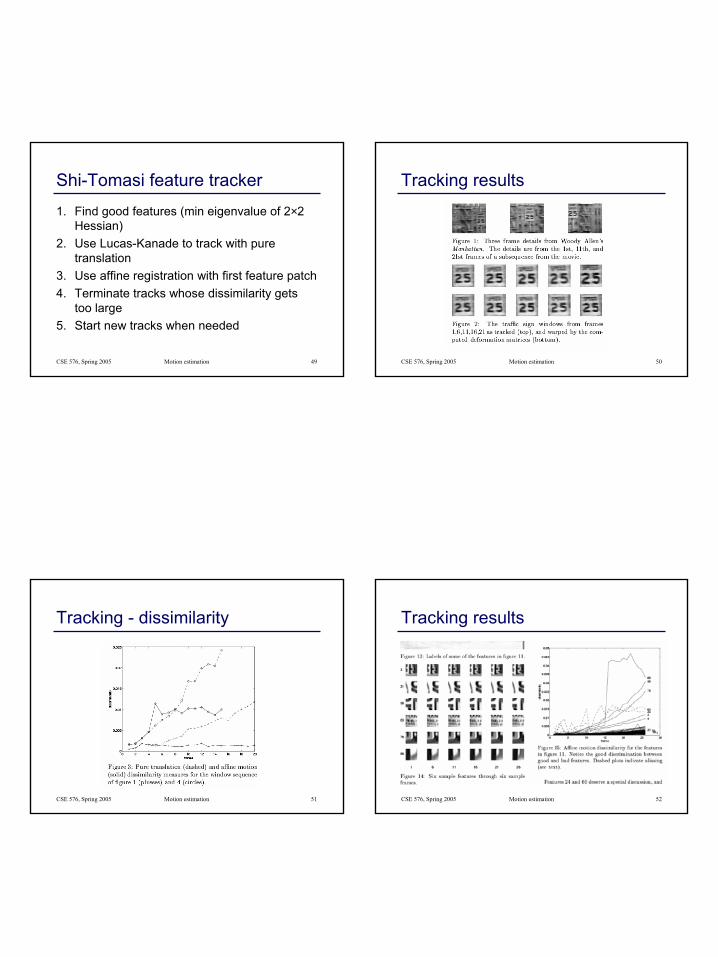
Shi-Tomasi feature tracker
1. Find good features (min eigenvalue of 2×2 Hessian)
2. Use Lucas-Kanade to track with pure translation
3. Use affine registration with first feature patch4. Terminate tracks whose dissimilarity gets
too large5. Start new tracks when needed
CSE 576, Spring 2005 Motion estimation 50
Tracking results
CSE 576, Spring 2005 Motion estimation 51
Tracking - dissimilarity
CSE 576, Spring 2005 Motion estimation 52
Tracking results
14
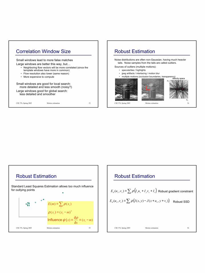
CSE 576, Spring 2005 Motion estimation 53
Correlation Window SizeSmall windows lead to more false matchesLarge windows are better this way, but…
• Neighboring flow vectors will be more correlated (since the template windows have more in common)
• Flow resolution also lower (same reason)• More expensive to compute
Small windows are good for local search:more detailed and less smooth (noisy?)
Large windows good for global search:less detailed and smoother
CSE 576, Spring 2005 Motion estimation 54
Robust EstimationNoise distributions are often non-Gaussian, having much heavier
tails. Noise samples from the tails are called outliers.Sources of outliers (multiple motions):
• specularities / highlights• jpeg artifacts / interlacing / motion blur• multiple motions (occlusion boundaries, transparency)
velocity spacevelocity space
u1
u2
++
CSE 576, Spring 2005 Motion estimation 55
Robust Estimation
Standard Least Squares Estimation allows too much influence for outlying points
)()
)()(
)()(
2
mxx
x
mxx
xmE
i
ii
ii
−=∂∂=
−=
=∑
ρψ
ρ
ρ
( Influence
CSE 576, Spring 2005 Motion estimation 56
Robust Estimation
( )∑ ++= tsysxssd IvIuIvuE ρ),( Robust gradient constraint
( )∑ ++−= ),(),(),( ssssd vyuxJyxIvuE ρ Robust SSD
15
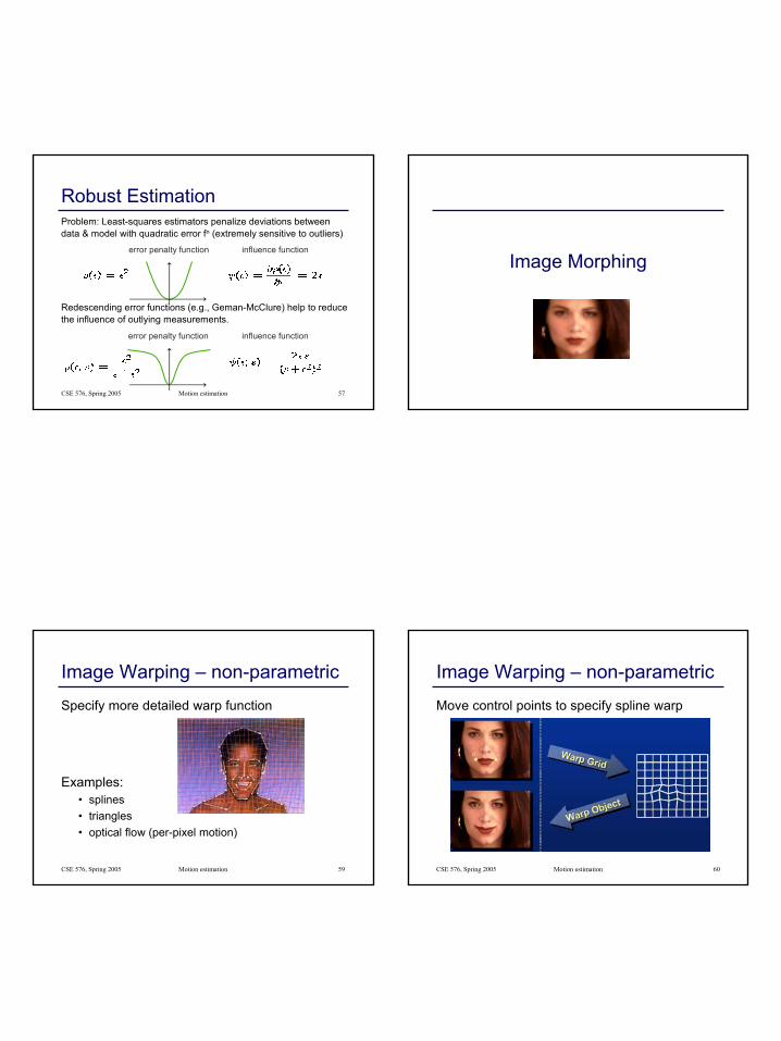
CSE 576, Spring 2005 Motion estimation 57
Robust EstimationProblem: Least-squares estimators penalize deviations between data & model with quadratic error fn (extremely sensitive to outliers)
error penalty function influence function
Redescending error functions (e.g., Geman-McClure) help to reduce the influence of outlying measurements.
error penalty function influence function
Image Morphing
CSE 576, Spring 2005 Motion estimation 59
Image Warping – non-parametric
Specify more detailed warp function
Examples: • splines• triangles• optical flow (per-pixel motion)
CSE 576, Spring 2005 Motion estimation 60
Image Warping – non-parametric
Move control points to specify spline warp
16
CSE 576, Spring 2005 Motion estimation 61
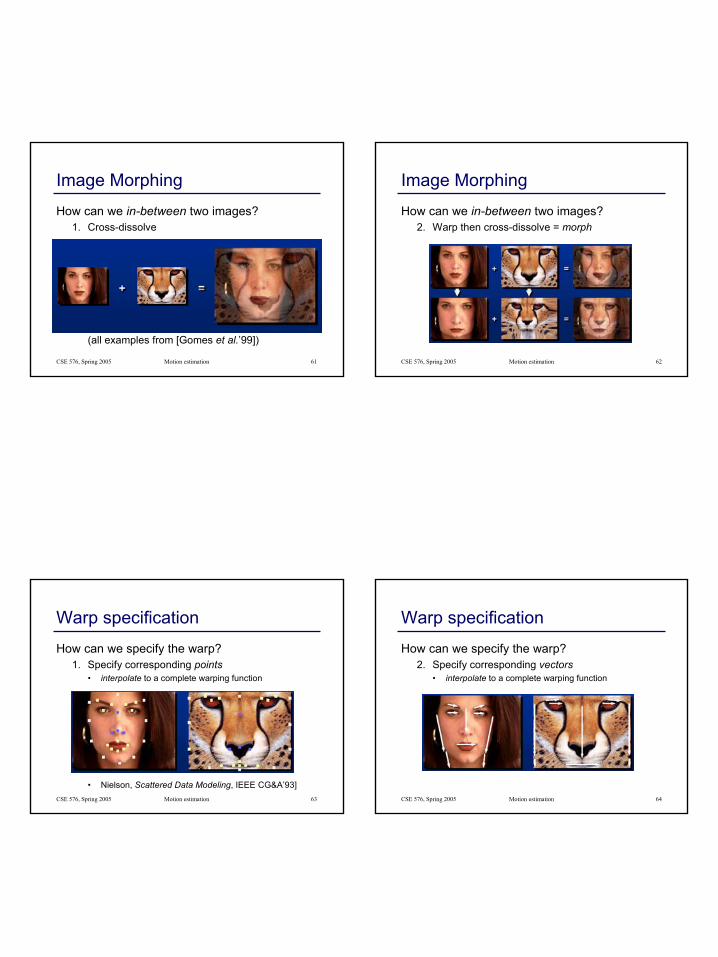
Image Morphing
How can we in-between two images?1. Cross-dissolve
(all examples from [Gomes et al.’99])
CSE 576, Spring 2005 Motion estimation 62
Image Morphing
How can we in-between two images?2. Warp then cross-dissolve = morph
CSE 576, Spring 2005 Motion estimation 63
Warp specification
How can we specify the warp?1. Specify corresponding points
• interpolate to a complete warping function
• Nielson, Scattered Data Modeling, IEEE CG&A’93]CSE 576, Spring 2005 Motion estimation 64
Warp specification
How can we specify the warp?2. Specify corresponding vectors
• interpolate to a complete warping function
17
CSE 576, Spring 2005 Motion estimation 65
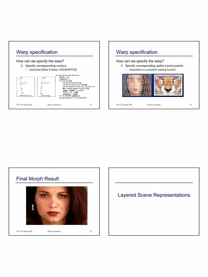
Warp specification
How can we specify the warp?2. Specify corresponding vectors
• interpolate [Beier & Neely, SIGGRAPH’92]
CSE 576, Spring 2005 Motion estimation 66
Warp specification
How can we specify the warp?3. Specify corresponding spline control points
• interpolate to a complete warping function
CSE 576, Spring 2005 Motion estimation 67
Final Morph Result
Layered Scene Representations
18
CSE 576, Spring 2005 Motion estimation 69
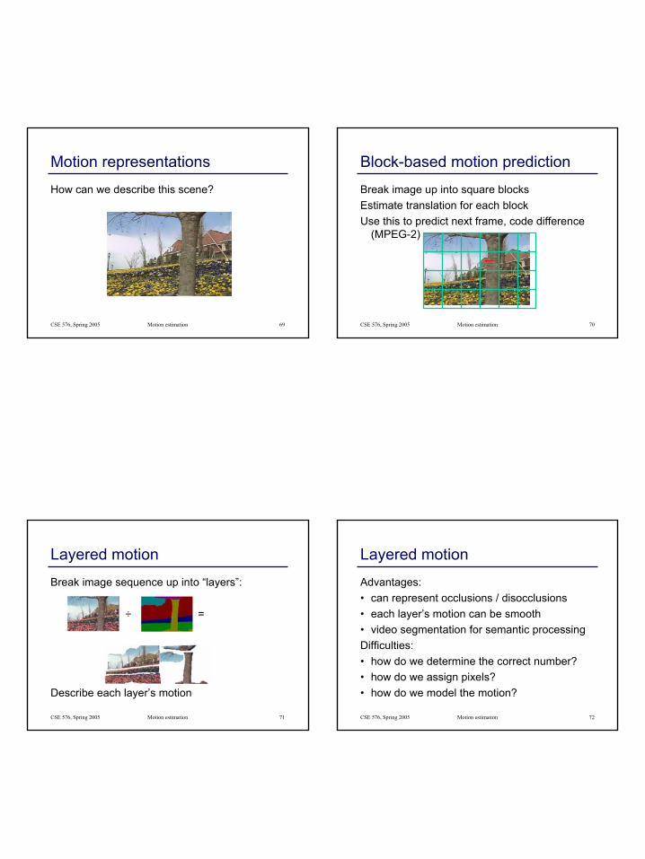
Motion representations
How can we describe this scene?
CSE 576, Spring 2005 Motion estimation 70
Block-based motion prediction
Break image up into square blocksEstimate translation for each blockUse this to predict next frame, code difference
(MPEG-2)
CSE 576, Spring 2005 Motion estimation 71
Layered motion
Break image sequence up into “layers”:
÷ =
Describe each layer’s motion
CSE 576, Spring 2005 Motion estimation 72
Layered motion
Advantages:• can represent occlusions / disocclusions• each layer’s motion can be smooth• video segmentation for semantic processingDifficulties:• how do we determine the correct number?• how do we assign pixels?• how do we model the motion?
19
CSE 576, Spring 2005 Motion estimation 73
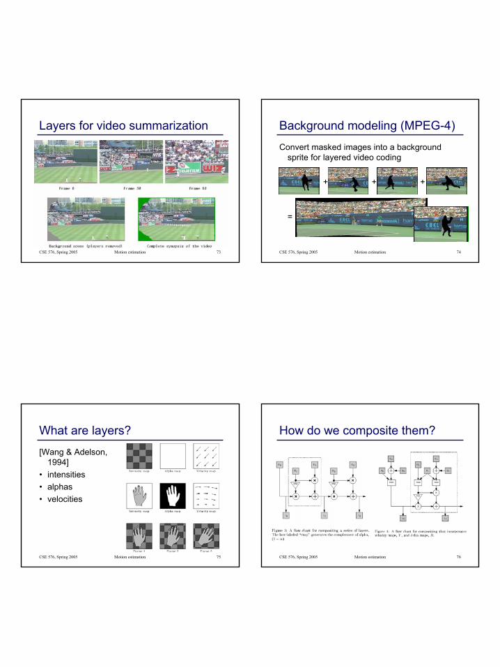
Layers for video summarization
CSE 576, Spring 2005 Motion estimation 74
Background modeling (MPEG-4)
Convert masked images into a background sprite for layered video coding
+ + +
=
CSE 576, Spring 2005 Motion estimation 75
What are layers?
[Wang & Adelson, 1994]
• intensities• alphas• velocities
CSE 576, Spring 2005 Motion estimation 76
How do we composite them?
20
CSE 576, Spring 2005 Motion estimation 77
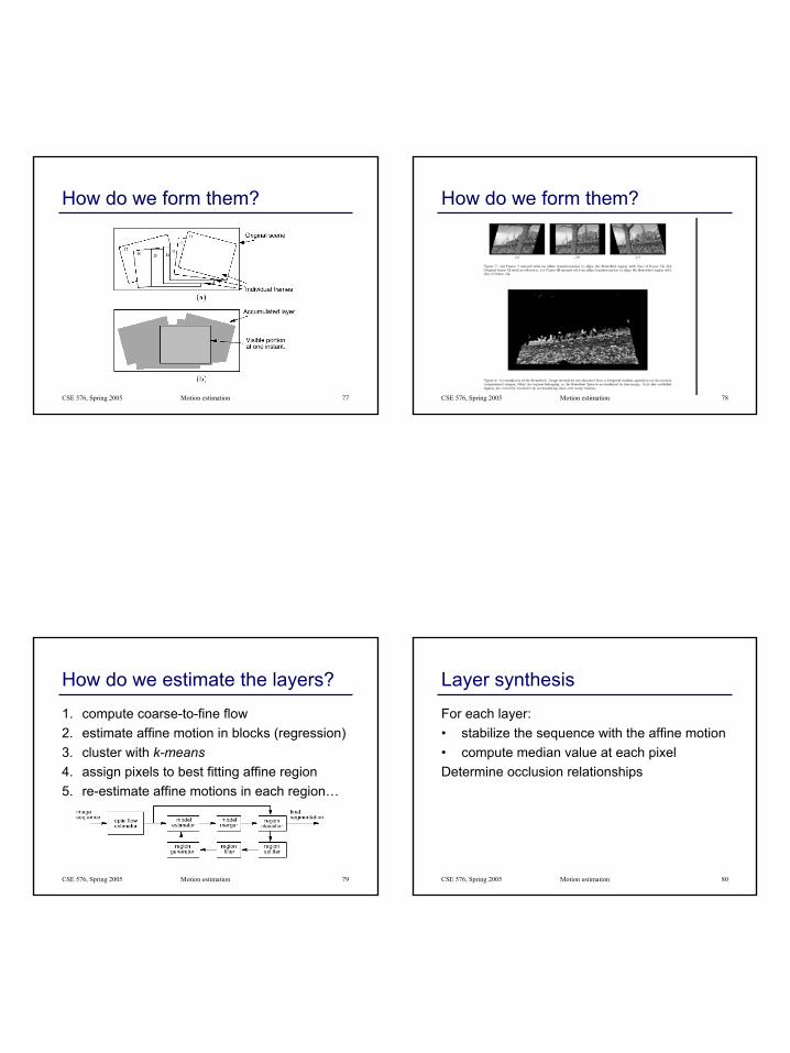
How do we form them?
CSE 576, Spring 2005 Motion estimation 78
How do we form them?
CSE 576, Spring 2005 Motion estimation 79
How do we estimate the layers?
1. compute coarse-to-fine flow2. estimate affine motion in blocks (regression)3. cluster with k-means4. assign pixels to best fitting affine region5. re-estimate affine motions in each region…
CSE 576, Spring 2005 Motion estimation 80
Layer synthesis
For each layer:• stabilize the sequence with the affine motion• compute median value at each pixelDetermine occlusion relationships
21
CSE 576, Spring 2005 Motion estimation 81
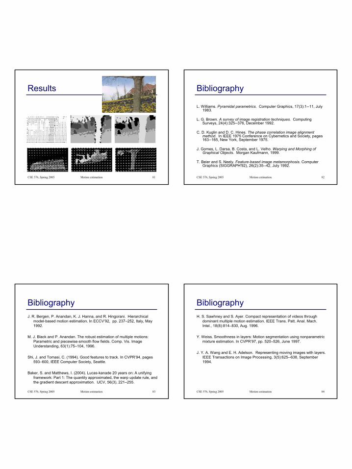
Results
CSE 576, Spring 2005 Motion estimation 82
Bibliography
L. Williams. Pyramidal parametrics. Computer Graphics, 17(3):1--11, July 1983.
L. G. Brown. A survey of image registration techniques. Computing Surveys, 24(4):325--376, December 1992.
C. D. Kuglin and D. C. Hines. The phase correlation image alignment method. In IEEE 1975 Conference on Cybernetics and Society, pages 163--165, New York, September 1975.
J. Gomes, L. Darsa, B. Costa, and L. Velho. Warping and Morphing of Graphical Objects. Morgan Kaufmann, 1999.
T. Beier and S. Neely. Feature-based image metamorphosis. Computer Graphics (SIGGRAPH'92), 26(2):35--42, July 1992.
CSE 576, Spring 2005 Motion estimation 83
BibliographyJ. R. Bergen, P. Anandan, K. J. Hanna, and R. Hingorani. Hierarchical
model-based motion estimation. In ECCV’92, pp. 237–252, Italy, May 1992.
M. J. Black and P. Anandan. The robust estimation of multiple motions: Parametric and piecewise-smooth flow fields. Comp. Vis. Image Understanding, 63(1):75–104, 1996.
Shi, J. and Tomasi, C. (1994). Good features to track. In CVPR’94, pages 593–600, IEEE Computer Society, Seattle.
Baker, S. and Matthews, I. (2004). Lucas-kanade 20 years on: A unifying framework: Part 1: The quantity approximated, the warp update rule, and the gradient descent approximation. IJCV, 56(3), 221–255.
CSE 576, Spring 2005 Motion estimation 84
BibliographyH. S. Sawhney and S. Ayer. Compact representation of videos through
dominant multiple motion estimation. IEEE Trans. Patt. Anal. Mach. Intel., 18(8):814–830, Aug. 1996.
Y. Weiss. Smoothness in layers: Motion segmentation using nonparametric mixture estimation. In CVPR’97, pp. 520–526, June 1997.
J. Y. A. Wang and E. H. Adelson. Representing moving images with layers. IEEE Transactions on Image Processing, 3(5):625--638, September 1994.

22
CSE 576, Spring 2005 Motion estimation 85
BibliographyY. Weiss and E. H. Adelson. A unified mixture framework for motion
segmentation: Incorporating spatial coherence and estimating thenumber of models. In IEEE Computer Society Conference on Computer Vision and Pattern Recognition (CVPR'96), pages 321--326, San Francisco, California, June 1996.
Y. Weiss. Smoothness in layers: Motion segmentation using nonparametric mixture estimation. In IEEE Computer Society Conference on Computer Vision and Pattern Recognition (CVPR'97),pages 520--526, San Juan, Puerto Rico, June 1997.
P. R. Hsu, P. Anandan, and S. Peleg. Accurate computation of optical flow by using layered motion representations. In Twelfth International Conference on Pattern Recognition (ICPR'94), pages 743--746, Jerusalem, Israel, October 1994. IEEE Computer Society Press
CSE 576, Spring 2005 Motion estimation 86
BibliographyT. Darrell and A. Pentland. Cooperative robust estimation using layers of
support. IEEE Transactions on Pattern Analysis and Machine Intelligence, 17(5):474--487, May 1995.
S. X. Ju, M. J. Black, and A. D. Jepson. Skin and bones: Multi-layer, locally affine, optical flow and regularization with transparency. In IEEE Computer Society Conference on Computer Vision and Pattern Recognition (CVPR'96), pages 307--314, San Francisco, California, June 1996.
M. Irani, B. Rousso, and S. Peleg. Computing occluding and transparent motions. International Journal of Computer Vision, 12(1):5--16, January 1994.
H. S. Sawhney and S. Ayer. Compact representation of videos through dominant multiple motion estimation. IEEE Transactions on Pattern Analysis and Machine Intelligence, 18(8):814--830, August 1996.
M.-C. Lee et al. A layered video object coding system using sprite and affine motion model. IEEE Transactions on Circuits and Systems for Video Technology, 7(1):130--145, February 1997.
CSE 576, Spring 2005 Motion estimation 87
BibliographyS. Baker, R. Szeliski, and P. Anandan. A layered approach to stereo
reconstruction. In IEEE CVPR'98, pages 434--441, Santa Barbara, June 1998.
R. Szeliski, S. Avidan, and P. Anandan. Layer extraction from multiple images containing reflections and transparency. In IEEE CVPR'2000, volume 1, pages 246--253, Hilton Head Island, June 2000.
J. Shade, S. Gortler, L.-W. He, and R. Szeliski. Layered depth images. In Computer Graphics (SIGGRAPH'98) Proceedings, pages 231--242, Orlando, July 1998. ACM SIGGRAPH.
S. Laveau and O. D. Faugeras. 3-d scene representation as a collection of images. In Twelfth International Conference on Pattern Recognition (ICPR'94), volume A, pages 689--691, Jerusalem, Israel, October 1994. IEEE Computer Society Press.
P. H. S. Torr, R. Szeliski, and P. Anandan. An integrated Bayesian approach to layer extraction from image sequences. In Seventh ICCV'98, pages 983--990, Kerkyra, Greece, September 1999.