NBER WORKING PAPER SERIES

WHY DO FIRMS OWN PRODUCTION CHAINS?

Enghin AtalayAli Hortacsu

Chad Syverson

Working Paper 18020http://www.nber.org/papers/w18020

NATIONAL BUREAU OF ECONOMIC RESEARCH1050 Massachusetts Avenue

Cambridge, MA 02138April 2012

Hortaçsu thanks the NSF (SES-1124073) and Syverson thanks the NSF (SES-0519062), the John M.Olin Foundation, and the Stigler Center for funding. The research in this paper was conducted whilethe authors were Special Sworn Status researchers of the U.S. Census Bureau at the Chicago CensusResearch Data Center. Research results and conclusions expressed are those of the authors and donot necessarily reflect the views of the Census Bureau. This paper has been screened to insure thatno confidential data are revealed. Support for this research at the Chicago RDC from NSF (awardsno. SES-0004335 and ITR-0427889) is also gratefully acknowledged. The views expressed hereinare those of the authors and do not necessarily reflect the views of the National Bureau of EconomicResearch.

NBER working papers are circulated for discussion and comment purposes. They have not been peer-reviewed or been subject to the review by the NBER Board of Directors that accompanies officialNBER publications.

© 2012 by Enghin Atalay, Ali Hortacsu, and Chad Syverson. All rights reserved. Short sections oftext, not to exceed two paragraphs, may be quoted without explicit permission provided that full credit,including © notice, is given to the source.

Why Do Firms Own Production Chains?Enghin Atalay, Ali Hortacsu, and Chad SyversonNBER Working Paper No. 18020April 2012JEL No. L0,L23,L24

ABSTRACT

We use broad-based yet detailed data from the economy’s goods-producing sectors to investigate firms’ownership of production chains. It does not appear that vertical ownership is primarily used to facilitatetransfers of goods along the production chain, as is often presumed: Roughly one-half of upstreamplants report no shipments to their firms’ downstream units. We propose an alternative explanationfor vertical ownership, namely that it promotes efficient intra-firm transfers of intangible inputs. Weshow evidence consistent with this hypothesis, including the fact that upon a change of ownership,an acquired plant begins to resemble the acquiring firm along multiple dimensions.

Enghin AtalayUniversity of Chicago1126 E 59th StreetChicago, IL 60637atalay@uchicago.edu

Ali HortacsuDepartment of EconomicsUniversity of Chicago1126 East 59th StreetChicago, IL 60637and NBERhortacsu@uchicago.edu

Chad SyversonUniversity of ChicagoBooth School of Business5807 S. Woodlawn Ave.Chicago, IL 60637and NBERchad.syverson@chicagobooth.edu

Many firms own links of production chains. That is, they operate both upstream and

downstream plants, where the upstream industry produces an input used by the downstream

industry. We explore the reasons for such ownership using two detailed and comprehensive data

sets on ownership structure, production, and shipment patterns throughout broad swaths of the

U.S. economy.

We find that most vertical ownership does not appear to be primarily concerned with

facilitating physical goods movements along a production chain within the firm, as is commonly

presumed. Upstream units ship surprisingly small shares of their output to their firms’

downstream plants. One-half of upstream plants do not report making shipments inside their

firm. The median internal shipments share across upstream plants in vertical production chains

is 0.4 percent, if shipments are counted equally, and less than 0.1 percent in terms of total dollar

values or weight. Even the 90th percentile internal shippers are hardly dedicated makers of

inputs for their firms’ downstream operations, with 38 percent of the value of their shipments

sent outside the firm. (However, a small fraction of upstream plants—slightly more than 1

percent—are operated as dedicated producers of inputs for their firms’ downstream operations,

and these plants tend to be quite large. We will discuss this further below.) These small shares

are robust to a number of choices we made about the sample, how vertical links are defined, and

whether we measure internal shares as a percentage of the firm’s upstream production or its

downstream use of the product.

This result raises a puzzle. If firms don’t own upstream and downstream units so the

former can provide intermediate materials inputs for the latter, why do they? Certainly, much of

the literature on vertical integration—stretching back to the landmark paper by Coase (1937),

with other notable later contributions like Stigler (1951), and Grossman and Hart (1986)—

couches firms’ motives for integrating in terms of facilitating movement of products along a

production chain.1 (Of course, in some contexts like hotel or business services franchising,

vertical integration often does not involve transfers of physical goods. Our paper, however,

focuses on vertically integration and shipments in the goods-producing sectors of the economy,

1 The size of the literature precludes comprehensive citation. Surveys include Perry (1989), Salop (1998), Joskow (2005), and Lafontaine and Slade (2007). Much of the recent industrial organization research on integration has focused on foreclosure (market power) implications. Examples of recent theoretical and empirical work with broader views of the determinants of integration within and across industries include Antras (2003), Acemoğlu, Johnson, and Mitton (2005) and Acemoğlu, Aghion, Griffith, and Zilibotti (2010).

2

like manufacturing. Our view is that a fair reading of the parables and case studies in the vertical

integration literature would imply that many, if not most, researchers would consider moderating

physical goods transactions a key motive for vertical ownership.)

We propose an alternative explanation that is consistent with small amounts of shipments

within vertically structured firms, and even with an absence of internal shipments altogether.

Namely, that the primary purpose of ownership is to mediate efficient transfers of intangible

inputs within firms. Managerial oversight and planning strike us as important types of such

intangibles, but these need not be involved. Other possibilities include marketing know-how,

intellectual property, and R&D capital, but any information-based input might be transferred

readily across upstream and downstream units.2

That vertical integration is often about transfers of intangible inputs rather than physical

ones may seem unusual at first glance. However, as observed by Arrow (1975) and Teece

(1982), it is precisely in the transfer of nonphysical knowledge inputs that the market, with its

associated contractual framework, is mostly likely to fail to be a viable substitute for the firm.

This, of course, does not preclude integration from also involving physical input transfers in

some cases. As noted above, we find a small number of plants that are clearly dedicated

producers for their firms’ downstream production units. However, these are the exception rather

than the rule. Thus it appears that the “make-or-buy” decision (at least referring to physical

inputs) can explain only a fraction of the vertical ownership structures in the economy.

We find additional patterns in the data that are consistent with the intangible inputs

explanation. First, we show that plants in vertical ownership structures have higher productivity

levels, are larger, and are more capital intensive than other plants in their industries. These

disparities, which we interpret as embodying fundamental differences in plant “type,” mostly

reflect persistent differences in plants started by or brought into vertically structured firms. In

other words, while there are some modest changes in plants’ type measures upon integration, the

cross sectional differences primarily reflect selection on pre-existing heterogeneity. Controlling

for firm size explains most of these type differences; plants of similarly-sized firms have similar

types, regardless of whether their firm is structured vertically, horizontally, or as a conglomerate.

Second, by studying how establishments’ behavior changes upon changes of ownership,

2 These inputs might be just as likely to be transferred from the firm’s “downstream” units to its “upstream” ones as vice versa. The names reflect the flow of the physical production process, not necessarily the actual flow of inputs within the firm.

3

we provide suggestive evidence of flows of intangible inputs within vertically structured firms.

Acquired establishments begin to resemble existing establishments in their acquiring firms along

two key dimensions: the acquired plants start shipping their outputs to locations that their

acquirers had already been shipping to, and begin producing products that their acquirers had

already been manufacturing.

These patterns evoke the equilibrium assignment view of firm organization advanced by

Lucas (1978), Rosen (1982), and more recently by Garicano and Rossi-Hansberg (2006) and

Garicano and Hubbard (2007). To the extent that intangibles are complementary to the physical

inputs involved in making vertically linked products, equilibrium assignment typically entails the

allocation of higher-type intangible inputs to higher-type plants in each product category. If

plant size is restricted by physical scale constraints, better intangible inputs will also be shared

across a larger number of plants. Simply put, higher-quality intangible inputs (e.g., the best

managers) are spread across a greater set of productive assets. Some of these assets can be

vertically linked plants, but their vertical linkage need not necessarily imply the transfer of

physical goods among them.

Furthermore, there may not be anything special about vertical structures per se. The

evidence below suggests that firm size, not structure, is the primary reflection of input quality.

Larger firms just happen to be more likely to contain vertically linked plants. In this way,

vertical expansion by a firm may not be altogether different than horizontal expansion. A typical

horizontal expansion involves the firm starting operations in markets that are new but still near to

its current line(s) of business, under the expectation that its current abilities can be carried over

into the new markets. Physical goods transfers among the firm’s establishments are not

automatically expected in such expansions, but inputs like management and marketing are

expected to flow to units in the new markets. Vertical expansions may operate similarly.

Industries immediately upstream and downstream of a firm’s current operations are obviously

related lines of business. Firms will occasionally expand into these lines, expecting their current

capabilities to prove useful in the new markets. And, just as with horizontal expansions,

transfers of managerial or other non-tangible inputs will be made to the new establishments. Yet

no physical good transfers from upstream to downstream establishments need occur.

The upshot is that the assignment view of the firm is consistent with large firms

composed of high-type plants operating (often) in several lines of business. Common ownership

4

allows the firm to efficiently move intangible inputs across its production units. Many of these

units will be vertically related, making these segments “vertical” in that the firm owns each end

of a link in a production chain. But the chain need not exist for the purpose of moderating the

flow of physical products along it.

This scenario is consistent with the evidence we document here, and in particular with

our primary result about the lack of goods shipments within vertically structured firms. The

remainder of the paper lays out the evidence and tests the hypothesis in more detail. It is

organized as follows. The next section describes our data sources. We then explain in Section

III how we use them to measure vertical integration and shipments internal and external to

vertical chains within firms. Section IV reports the empirical results. Section V discusses flows

of intangible inputs across establishments, within firms. We conclude in Section VI.

I. Data

We use microdata from two sources, the U.S. Economic Census and the Commodity

Flow Survey, and aggregate data from the Annual Wholesale Trade Survey and the Annual

Retail Trade Survey. We discuss each dataset in turn.

Economic Census. The Economic Census (EC) is an establishment-level census that is

conducted every five years, in years ending in either a “2” or a “7”. Establishments are unique

locations where economic activity takes place, like stores in the retail sector, warehouses in

wholesale, offices in business services, and factories in manufacturing. Our sample uses

establishments from the 1977, 1982, 1987, 1992, and 1997 censuses. We specifically use those

establishments in the Longitudinal Business Database, which includes the universe of all U.S.

business establishments with paid employees.3 The data has been reviewed by Census staff to

ensure that establishments can be accurately linked across time and that their entry and exit have

been measured correctly.

Critically, the Economic Census contains the owning-firm indicators necessary for us to

identify which plants are vertically integrated. (We discuss in Section III how we make this

classification.) Additionally, the Census of Manufactures portion of the EC also contains

3 Plant-level data from before 1977 is almost exclusively for the manufacturing sector, precluding proper classification of vertical ownership for manufacturing plants owned by firms that are in fact vertically structured, but only into non-manufacturing sectors (e.g., firms that own a manufacturing plant and a retail store selling the product the plant makes).

5

considerable data on plants’ production activities. This includes information on their annual

value of shipments, production and nonproduction worker employment, capital stocks, and

purchases of intermediate materials and energy. We use this production data to construct plant-

specific output, productivity, and factor intensity measures; details are discussed further below

and in the Appendix. In some cases, we augment the base production data with microdata from

the Census of Manufactures materials supplement, which contains, by plant, six-digit SIC

product-level information on intermediate materials expenditures.4

Commodity Flow Survey. The Commodity Flow Survey (CFS) collects data on

shipments originating from mining, manufacturing, wholesale, and catalog and mail-order retail

establishments.5 The survey defines shipments as “an individual movement of commodities

from an establishment to a customer or to another location in the originating company.” The

CFS takes a random sample of an establishment’s shipments in each of four weeks during the

year, one in each quarter. The sample generally includes 20-40 shipments per week, though

establishments with fewer than 40 shipments during the survey week simply report all of them.

For each shipment, the originating establishment is observed, as well as the shipment’s

destination zip code (exports report the port of exit along with a separate entry indicating the

shipment as an export), the commodity, the mode(s) of transportation, and the dollar value and

weight of the shipment.

We use the microdata from the 1993 and 1997 CFS; the former contains roughly 120,000

establishments and 11 million shipments, and the latter 60,000 establishments and 5.5 million

shipments. As with the Economic Census, each establishment has an identification number

denoting the firm that owns it. Both the establishment and the firm numbers are comparable to

those in the EC, so we can merge data from the two sources. We match the 1993 CFS to the

1992 EC; this will inevitably lead to some mismeasurement of ownership patterns, but we expect

this will be small given the modest annual rates at which plants are bought and sold by firms.

4 For very small EC plants, typically those with less than five employees, the Census Bureau does not elicit detailed production data from the plants themselves. It instead relies on tax records to obtain information on plant revenues and employment and then imputes all other production data. We exclude such plants—called Administrative Records (AR) plants—from those analyses below that use plant-level measures constructed from the Census of Manufactures (e.g., productivity). While roughly one-third of plants in the Census of Manufactures are AR plants, their small size means they comprise a much smaller share of industry-level output and employment aggregates. 5 Hillberry and Hummels (2003, 2008) and Holmes and Stevens (2010, 2012) use the CFS microdata to investigate various affects of distance on trade patterns. They do not make the within- and between-firm distinctions that we do here. These are the only other studies using the CFS microdata that we are aware of.

6

Annual Wholesale Trade Survey and Annual Retail Trade Survey. These datasets provide

information on sales and purchases of 4-digit retail and wholesale industries. We use these

datasets to help determine whether two industries are vertically linked.

II. Measuring Vertical Ownership and Shipments within Firms’ Production Chains

This section explains how we use our data to determine which businesses are vertically

integrated and whether the CFS shipments we observe are internal or external to the firm.

Determining Which Industries Are Vertically Linked to One Another

We define vertically linked industries as I-J industry pairs for which a substantial

fraction—1% in the baseline specification—of industry I’s sales are sent to establishments in

industry J. 6 To compute the fraction of sales of industry I output that are sent to industry J, we

use information from the 1992 Bureau of Economic Analysis Input-Output Tables, the 1992

Economic Census, the 1993 Commodity Flow Survey, the1993 Annual Wholesale Trade Survey,

and the 1993 Annual Retail Trade Survey. We define industries by their 4-digit SIC code. We

apply the classification of vertically linked industries implied by this data to our entire sample.7

To measure the value of shipments sent by industry-I establishments to industry-J

establishments, we first compute the shipments of commodity C sent to industry J using the 1993

CFS. Commodities are defined by their Standard Transportation Commodity Code (STCC).8

We then sum over all commodities that each industry I ships to determine the share of I’s sales

going to J, thereby indicating which I-J industry pairs are vertically linked.

For most industries, we rely primarily on the Input-Output Tables, which track quantities

of inter-industry flows of goods and services, to perform these calculations. However, the I-O

Tables treat the entire wholesale sector as a single, monolithic industry, with no distinction as to

the types of products its establishments distribute. They treat the retail sector in the same way.

6 The one-percent cutoff used to define substantial vertical links is of course arbitrary. We have checked our major findings using a five-percent cutoff and found few differences. (The overall level of integration is of course lower in this more stringent case.) 7 Applying one vertical structure to the entire sample is made necessary by the lack of CFS microdata before 1993 and changes in the way the CFS records commodities between 1993 and 1997. Given that the input-output structure of the economy is fairly stable over time, we do not expect a large impact on our results. 8 A list of STCC codes can be found in pages 117 to 167 of “Reference Guide for the 2008 Surface Transportation Board Carload Waybill Sample,” published by Railinc.

7

Additionally, they do not keep track of shipments by manufacturers to (or through) wholesalers

or retailers, instead measuring only those inputs directly used by wholesalers and retailers in the

production of wholesale and retail services (e.g., in the I-O Tables, cardboard boxes are a major

input used by the wholesale sector, but the actual products the sector distributes are not). To

achieve better measurement of the flow of goods through the wholesale and retail sector, we use

a different algorithm that incorporates additional data from the Annual Wholesale Trade Survey

and the Annual Retail Trade Survey. All these calculations are detailed in the Appendix.9

Classifying Shipments as Internal or External to the Firm

To classify shipments from vertically integrated establishments in the Commodity Flow

Survey as internal or external to the firm, we first must merge the CFS and EC data. This can be

done straightforwardly using the two datasets’ common establishment and firm identifiers. Of

critical importance is the fact that the Commodity Flow Survey contains the destination zip code

of each shipment, while the Economic Census records establishments’ zip codes.

We identify a shipment as internal if the shipping establishment’s firm also owns an

establishment that is both in the destination zip code and in a 4-digit SIC industry that is a

downstream vertical link (as defined above) of the sending establishment’s industry.10 The CFS

contains shipment-specific sample weights that indicate how many actual shipments in the

population each sampled shipment represents. We use these weights when computing the shares

of internal shipments, be it by count, dollar value, or weight.

III. Shipments within Firms’ Vertical Links

We begin by looking at the patterns of shipments within firms’ vertical links. We focus

on establishments in the Commodity Flow Survey that are a) in vertical ownership structures and

b) upstream links within those structures.

9 In a previous draft, we employed a cruder methodology to identify pairs of vertically linked industries, defining industry I as upstream of industry J provided either a) J buys at least five percent of its intermediate materials from I, or b) I sells at least five percent of its own output to industry J. We furthermore did not attempt to make any distinction among wholesale or retail industries. While we prefer the current methodology for its increased accuracy, we reproduce our main analysis using the old methodology in the Appendix and find similar results. 10 Every establishment is assigned to a unique industry. For establishments that produce products that fall under multiple 4-digit SIC industries, the Census Bureau classifies such plants based on their primary product, which is almost always the product accounting for the largest share of revenue.

8

A. Vertically Integrated Establishments’ Shipments—Benchmark Sample

The combined 1993 and 1997 CFS yield a core sample of about 67,500 plant-year

observations of upstream establishments in firms’ production chains. These establishments

report a total of roughly 6.3 million shipments in the CFS. Panel A of Table 1 shows the

prevalence of internal shipments within this sample. It reports quantiles of the distribution of

internal shipment shares across our sample plants, measured as the fraction of the total number,

dollar value, and weight of the establishment’s shipments.11

Overall, only a small share vertically integrated upstream establishments’ shipments are

to downstream units in the same firm. Across the 67,500 establishments, the median fraction of

internal shipments is 0.4 percent. The median internal shares by dollar value and weight are

even smaller, at less than 0.1 percent. Almost half of the plants report no internal shipments at

all. Even the 90th-percentile plant ships over 60 percent of its output outside the firm.

The exception to this general pattern is the small set of establishments that are clearly

dedicated to serving the downstream needs of their firm, the 1.2 percent of the sample that

reports exclusively internal shipments. The unusualness of this specialization is even more

apparent in the histogram of plants’ internal shipment shares shown in Figure 1, panel A. The

histogram echoes the quantiles reported above: the vast majority of upstream plants make few

internal transfers. The fractions of establishments fall essentially monotonically as internal

shipment shares rise—until the cluster of internally dedicated establishments. Another factor in

the unusualness of these internal specialist plants that is not apparent in the histogram is that they

are larger on average. This, along with the internal share distribution being highly skewed,

explains why the aggregate internal share of upstream plants’ shipments (the across-plant sum of

internal shipments divided by the across-plant sum of total shipments) is 16 percent. This is well

above the median share across plants. Thus internal shipments are more important on a dollar-

weighted than an ownership-decision-weighted basis, but are the exception in either case.

These results imply the traditional view that firms choose to own plants in upstream

industries to control input supplies may be off target. Clearly other motivations for ownership

must apply for those plants making no internal shipments. Even for those that do serve their own

11 For data confidentiality reasons, the reported quantiles are actually averages of the immediately surrounding percentiles; e.g., the median is the average of the 49th and 51st percentiles, the 75th percentile is the average of the 74th and 76th percentiles, and so on.

9

firm, though, their typically small internal shipments suggest that this role may not be primary.12

B. Robustness Checks

The disconnect between the upstream plants and their downstream partners, at least in

terms of physical goods transfers, is stark and perhaps surprising. We conduct several robustness

checks to verify our benchmark results.

First, it is appropriate to review some details of how the Commodity Flow Survey is

conducted, specifically with regard to its ability to capture intra-firm shipments. The CFS

definitely seeks to measure them, and it makes no distinction between intra- and inter-firm

transfers in its definition of “shipment.” In fact, the survey instructions (U.S. Census Bureau

(1997)) state explicitly that respondents should report shipments “to another location of your

company,” save for incidental items like “inter-office memos, payroll checks, business

correspondence, etc.”

There are several reasons to believe the implied shipments totals are accurate. First, the

Census Bureau audits responses by comparing the establishment’s implied annual value of

shipments from the CFS with that from other sources. If the disparity is well beyond statistical

variance, the Bureau contacts the respondent and reviews the responses for accuracy. If

integrated establishments were systematically underreporting internal shipments because of

confusion or by not following directions, the auditing process would help catch this.

Second, most establishments do report some internal shipments, indicating that they have

not interpreted the definition of shipments as precluding intra-firm transfers. This is also

reflected in the small share of establishments that report nothing but internal shipments.

Moreover, there is no mechanical reason why we should find the bump up in internal shipment

shares near one, as seen in Figure 1. We take this as further evidence that respondents

understand the CFS instructions.

Third, for plants in the manufacturing sector, there is an independent measure of internal

shipments. The Census of Manufacturers collects data on what it terms plants’ Interplant

Transfers, shipments that are sent to other plants in the same firm for further assembly. These

interplant transfers represent part, but not all, of our internal shipments measure—for example, 12 It is possible in some production chains that an upstream plant could completely serve its firm’s downstream needs with only a small fraction of its output. We show that this possibility is not driving our results in Appendix B3, however.

10

shipments to wholesalers or retailers are not included in CM Interplant Transfers.13 In addition to

the difference in definition, these measures are collected using separate survey instruments (often

likely to have been filled out by different individuals at the plant). Despite these differences, we

find a strong correlation between the two measures. The correlation coefficient between plants’

logged interplant transfers and our CFS-based estimate of internal shipments is 0.52 across our

matched sample of about 37,000 plant-years, and a regression of the latter on the former yields a

coefficient of 0.470 (s.e. = 0.011).

B.1. Robustness: Sample

In our first series of robustness checks, we consider the impact of modifications to our

core sample of upstream vertically integrated plants. The corresponding distributions of

establishments’ internal shipments are shown in Table 3, panel B. Each row is a separate check.

We show only the distributions of the dollar value shares for the sake of brevity; similar patterns

are observed in the shares by shipment counts or total weight.

The robustness check in the first row of panel B uses only establishments reporting at

least the median number of shipments across all establishments in the sample. The point is to

exclude those for which sampling error could be higher and for whom extreme values like zero

are more likely. This leaves us with a sample of about 34,000 establishment-years making just

over 4.2 million shipments. (This is greater than half the establishment-years in the benchmark

sample because several plants report exactly the median number of shipments.) Extreme values

are in fact rarer in this sample: 45.5 percent report making no internal shipments, down from 49

percent in the full sample, and 0.3 percent report exclusively internal shipments, down from 1.2

percent. The remainder of the distribution is not much different, however. The median fraction

of internal shipments is 0.2 percent, and the 90th percentile establishment is less likely to ship

internally than that in the full sample, with just under half of shipments being intra-firm.

The second check drops any establishment that reports any shipments for export. In the

CFS, the destination zip code of shipments for export is for the port of exit, with a separate note

indicating the shipment’s export status and its destination country. Thus internal shipments to a

firm’s overseas locations would be misclassified as outside the firm, unless by chance the firm 13 Restricting shipments to those that are sent for further assembly has a substantial impact on the estimate of plants’ internal shipments. We estimate in Appendix B1 that half of our measured internal shipments from manufacturing plants are sent to plants outside of the manufacturing sector (and, thus, are not for further assembly).

11

has a downstream establishment in the port’s zip code. Focusing on the roughly 47,000

establishments reporting no exports among their roughly 4.3 million shipments avoids this

potential mismeasurement. The results are in the second row of panel B of Table 3. The entire

distribution is close to the benchmark results above, with the median internal share being less

than 0.1 percent and 49.7 percent of establishments reporting zero intra-firm shipments. Missing

export destinations are not the source of our results.14

The next check counts shipments destined for the zip code of any plant in the same firm

as internal, not just those going to locations of downstream links of vertical chains. It is possible

that some vertical production may occur outside those chains we identify using the Input-Output

Tables. Some may even occur within a given industry, when a particularly complex production

process is broken up across multiple establishments. Here, we are taking the broadest possible

view toward defining intra-firm transfers of physical goods along a production chain. As seen in

the third row of panel B, all quantiles have internal shipment fractions higher than the

benchmark, as they must. Still, the median internal share is only 4.9 percent, and the 90th

percentile 67.5 percent. About 23 percent of establishments still have no shipments to a zip code

of any plant in their firm, and exclusively internal establishments number 2.7 percent.

In the fourth check we make the generous assumption that a shipment is internal if it goes

to any county in which the firm has a downstream establishment. While unrealistic, this

approach accounts for almost any problems with zip code reporting errors or missing zip codes.

The results of this exercise are in row 4 of panel B. Not surprisingly, the shares of shipments

considered intra-firm are considerably higher, given the easier criterion for being defined as

internal. There are more internal specialists or near-specialists: the 90th percentile internal share

is 87 percent, and 4.2 percent of establishments have all of their reported shipments being

internal. Even so, a substantial fraction of establishments—25 percent, more than five times the

number of internal specialists—report no shipments to counties where downstream plants in their

firms are located. The median internal share across plants is 7.2 percent.

The fifth check restricts the sample to plants in the twenty-five manufacturing industries

with the least amount of product differentiation, as measured by the Gollop and Monahan (1991)

product differentiation index. The concern is that even our detailed industry classification

14 We will discuss below how the fraction of international trade that is within firms could be so much larger than the intra-firm domestic trade we document here.

12

scheme may be too coarse to capture the true extant vertical links. For instance, it might be that

while two industries are substantially linked at an aggregate level, this actually reflects the

presence of (say) two separate vertical links within a four-digit SIC industry. In this case, we

would not expect many shipments to go from upstream plants in one link to downstream plants

in another, even though we might infer the two are vertically linked just from comparing the

industry-level trade patterns. Selecting industries with undifferentiated products should reduce

product heterogeneity within detailed industries and raise the probability that the industry links

we identify as described above hold at a disaggregate level. There are about 2200 plant-years in

this subset of industries in the CFS. We find that internal shares are actually lower for plants in

the less differentiated industries. The median plant has no internal shipments, while the 90th

percentile plant’s internal share is 20 percent

The remaining robustness checks in the panel explore the impact of varying the definition

of vertical links. Row 6 of the table shows the results using a 5 percent cutoff, while Row 7

keeps the 1 percent cutoff, but removes the possibility that an industry can be vertically linked

with itself. Both of these robustness checks reduce the number of plants that are defined to be

vertically linked from the benchmark. The 5 percent cutoff sample contains about 53,000 plant-

years and 5.0 million shipments, while the “No I → I” rule produces a sample with about 43,000

plant-years and 4.0 million shipments. In both these subsamples, the median and 90th percentile

internal shares are slightly smaller than in the benchmark.

All in all, our benchmark results appear robust to several sample and variable definition

changes. Additional robustness checks along these lines are provided in Appendix B1.

B.2. Robustness: Accounting for Actual Downstream Use

We measure internal shipments above as an upstream plant’s internal shipments as a

share of its total shipments. There are cases where this ratio might be misleading as to the extent

of intra-firm product movements. Consider a hypothetical copper products company with two

plants: an upstream mill that produces copper billets, and a downstream plant that processes

billets into pipe. Suppose the downstream plant needs $10 million of billets to operate at

capacity. Now say the upstream mill produced $100 million of billets in a year. If the mill

shipped $10 million of billets to the pipe-making plant and the remaining $90 million elsewhere,

we would compute its internal shipment share as 10 percent. Yet the firm would be completely

13

supplying its downstream needs internally. The difference in the scales of operations upstream

and downstream creates this misleading internal share.

While this may raise the question of why the firm wouldn’t own enough pipe plants to

use its upstream production, in this section we create an alternative measure of internal shipment

shares that can account for inherent differences in operating scales across industries. Instead of

using upstream plants’ total shipments as the denominator in the internal shipment share

measure, we instead calculate firms’ downstream use of products they make upstream. We then

construct internal shipments shares as intra-firm shipments of upstream plants divided by the

minimum of two values, either the firm’s total upstream shipments as above, or the firm’s

reported downstream use of the upstream product. Hence the internal share of the hypothetical

copper firm above would be 100%, rather than 10% as before, because the firm provides all the

copper it uses downstream.

While the CFS offers a random sample of establishments’ shipments, we unfortunately

do not have a random sample of establishments’ incoming materials. This precludes us from

directly measuring “internal purchase shares” in the same way we measure internal shipment

shares. But for a subset of firms we can construct internal shipments as a fraction of downstream

use. To do so, we must first restrict our CFS sample to those where we observe all the upstream

shipments of a firm, at least for a given product. If firms served downstream needs from

upstream plants not in the CFS, we would not observe their non-CFS plants’ shipments, and

therefore would not know they are internal. Hence we look here only at CFS plants where we

observe all the firm’s plants in a particular industry. We use the Economic Census to find this

subset of establishments, which ends up being about 11,000 plant-years. If we calculate these

shares as before, this subsample looks similar to the entire sample. For example, 53.8 percent of

these plants report making no internal shipments, and the 90th percentile plant ships 36.5 percent

of its output internally.

We then match these upstream plants’ shipments to downstream usage within the firm.

We construct three downstream usage measures. The first simply aggregates the materials

purchases of all the firm’s downstream manufacturing plants. These purchases are reported by

every plant in the Census of Manufactures. The firm’s downstream use of upstream products is

simply the sum of all its intermediate materials purchases. We can compute these downstream

use measures for 4438 firm-year observations. To compute internal shares, we add up the

14

internal shipments of the firms’ upstream plants to use as the numerator.15

The second measure of downstream usage matches upstream shipments to downstream

usage by product. We use the detailed materials purchase information from the Census of

Manufactures materials supplement, which collects plants’ materials purchases by detailed

product. We compute firm’s upstream shipments by product using the shipment commodity

codes available in the CFS. Product-specific shipments are computed at the 2-digit level. (We

use only 1993 CFS data here because a change in the commodity coding scheme made it difficult

to match the 1997 CFS commodity codes with the materials codes in the Census of

Manufactures.) We sum the same firm’s reported downstream use of that 2-digit product from

the Census of Manufactures. The internal shipment share is the ratio of the firm’s internal

shipments of the product divided by its reported downstream use of that product. We are able to

match 5491 firm-material combinations.

The third and final measure of downstream materials usage repeats the procedure above,

except matches at the more detailed 4-digit product level. Because the greater detail makes

finding matches less likely, we have a sample of 2351 such firm-product combinations.

The results from these exercises are shown in Table 2. Recall that we now compute

internal shipments as their share of the smaller of a) the firm’s (or firm-product’s) total upstream

shipments or b) the firm’s downstream usage. Again, only the dollar-value shares are shown for

brevity. The first row shows shares computed using the firm-level match where internal

materials usage is aggregated across all materials. The second row shows results from the

sample of matched firm-products at the 2-digit level; the third shows the firm-product match

sample at the 4-digit level.

All three measures downstream usage still imply that most vertical ownership structures

are not about serving the downstream material needs of the firm. The median share across plants

15 There are two measurement problems with this first approach that will tend to bias our internal shares measures in opposite directions. First, because we only required that we observe all of a firm’s plants making a particular product in the CFS, we might be missing internal shipments from firms’ other upstream plants (this is much less of a problem in our other two downstream use measures below, since they are matched by firm-product, rather than just by firm). This will cause us to understate the true internal shipment share. The second measurement issue arises because we can only observe materials purchases for downstream establishments in the manufacturing sector. If some upstream products are used in the firms’ non-manufacturing establishments, we will not include these in our downstream usage measures. This will lead us to overstate internal shipment shares. As a practical matter, both of these measurement concerns are probably second-order. Our restricted sample has a large fraction of firms with only a few establishments, so if a firm’s upstream plant(s) is in the CFS and its downstream plant(s) in manufacturing, chances are those are all the plants the firm owns.

15

of internal shipments as a fraction of the smaller of the firm’s upstream shipments and its

downstream use is 0.3% in the first (firm-wide) downstream use measure. The share of this

subsample reporting zero internal shipments is 44.4 percent. For the second measure of internal

usage (firm-product matching at the 2-digit level), 60.2 percent of the firms report no internal

shipments. For the third measure (firm-product matching at the 4-digit level), 65.3 percent of the

sample report no internal shipments.

One thing to note about the results is that some shares are above one. It is possible that

this reflects in part the fact that some of the upstream plants’ shipments that we classified as

internal because their destination zip code was where the firm owned a downstream plant in fact

went to a plant outside the firm in the same zip code. But probably some of these shares reflect

measurement error in firms’ downstream materials use (it is outside the manufacturing sector and

we can’t observe it, for instance). A summary measure of the extent of such measurement error

is the fraction of observations with implied internal usage ratios above one. For the three

downstream use measures above, these shares are 6.7, 11.7, and 12.5 percent, respectively.

Thus the small internal shares we were finding before do not seem to be simply reflecting

the fact that most integrated structures have considerably larger upstream plant scales than

downstream. In fact, we still find a large number of cases (slightly under one-half of the sample)

without any intra-firm shipments. In other words, we know a firm makes a particular product

upstream, uses that same product as an input downstream, but does not ship any of its own

upstream output to its downstream units.

B.3. Shipments of Plants that Make Firms Become Vertically Structured

We next look at the internal shipment patterns for a very select subset of establishment-

years in our sample. These observations have two properties. First, they correspond to newly

vertically integrated establishments on the upstream end of a production chain (they were single-

unit firms in the previous Economic Census). Additionally, these establishments have been

acquired by firms that, concurrent with the purchase, begin owning plants in a vertical

production chain for the first time. In other words, these are the establishments that make these

firms vertically structured. These establishments might provide one of the clearest windows into

any connection between why firms expand vertically and internal shipment patterns. Because of

the narrow selection criteria, the subsample is small—a total of just over 300 establishment-years

16

in the CFS, reporting about 28,000 shipments—but this still offers enough leverage to make a

meaningful comparison to the overall patterns discussed above.

This subsample exhibits an even lower prevalence of internal shipments than in the

benchmark. 68 percent of these plants report no internal shipments at all, and the 90th percentile

of internal shipments is only 10.1 percent. Because the small sample raises questions of whether

these differences are statistically significant, we also estimate regressions that project plants’

intra-firm shipment shares on an indicator for these new-VI establishment/firm units and full set

of industry-year dummies. The estimated coefficient on the subsample indicator in the dollar-

value-share regressions is -0.057 (s.e. = 0.009). (The coefficient is also significantly negative

when shares of shipment counts or weights are used as the dependent variable.) These

establishments do in fact have significantly lower internal shipments shares.

Thus even for establishments acquired expressly as part of a firm’s move to build a

vertically integrated ownership structure, internal sourcing of physical inputs is unusual.

B.4. Other Robustness Checks

We conducted additional, detailed robustness checks on the benchmark results that, for

the sake of brevity, we detail in the Appendix. One explores whether the observed small internal

shipment shares reflect the fact that plants in vertical ownership structures are spaced further

apart geographically than typical. We show this is not the case; in fact, even vertically structured

firms with all their plants in a single metro have internal shares similar to those in the broader

sample. A second robustness check asks whether our definition of vertical ownership, which by

necessity requires a firm to operate the upstream and downstream stages of production in

separate plants, misses vertically integrated production practices occurring within a single plant

(and therefore undercounting the within-plant “shipments” that accompany them). We find no

evidence that this is driving our result.

IV. Explanations for Vertical Ownership

The lack of movement of goods along production chains within most vertically structured

firms appears to be a robust feature of the data. As mentioned above, we propose that vertical

ownership is instead typically used to facilitate movements of intangible inputs like management

oversight across a firm’s production units. In this section we document additional facts that are

17

consistent with this theory.

A. Firms as Outcomes of an Assignment Mechanism

We first show evidence that plants’ vertical ownership structures are systematically

related to persistent differences in plant “types”—combinations of idiosyncratic demand and

supply fundamentals that affect plant profitability in equilibrium. Further, these type differences

primarily reflect “selection” on pre-existing differences rather than “treatment” effects of

becoming part of a vertical ownership structure. At the same time, we find that these type

differences aren’t much tied to vertical ownership itself, but rather to being in large firms of any

structure. We discuss below how these patterns are all consistent with theories of the firm as the

outcome of an assignment mechanism that allocates tangible and intangible assets among

heterogeneous firms. Models of such mechanisms—which include Lucas (1978), Rosen (1982),

and more recently by Garicano and Rossi-Hansberg (2006) and Garicano and Hubbard

(2007)16—offer an explanation for why we might not see many internal shipments within vertical

ownership structures while at the same time pointing us toward an alternative explanation for

such ownership patterns: namely, facilitating the flow of intangible inputs within the firm.

A.1. Plants in Vertical Ownership Structures are High “Type” Plants

We first focus on the patterns of plant-level measures of “type” across vertically

integrated and unintegrated plants. We use four measures to proxy for plant type.17 They are not

independent, but they differ enough in construction to allow us to gauge the consistency, or lack

thereof, of our results. Two are productivity measures that differ in their measure of inputs:

output per worker-hour and total factor productivity (TFP). (Both are expressed as the log of the

plant’s output-input ratio.) Our third type measure is simply the plant’s logged real revenue.

The fourth metric is the plant’s logged capital-labor ratio (capital stock per worker-hour).

Further details on the construction of these measures are in the Appendix. Because of data

limitations, we can only construct these measures for the roughly 350,000 plants in each Census

of Manufactures.

16 These models are in turn built on foundations laid out earlier by Koopmans’ (1951) and Becker (1973). 17 Foster, Haltiwanger, and Syverson (2008) present a model of industry equilibrium where producers differ along both demand and cost dimensions, and show that plant type can be summarized as a single-dimensional index of demand, productivity, and factor price fundamentals.

18

These empirical type measures have been shown in various empirical studies to be

correlated with plant survival. Survival probabilities reflect plant type in many models of

industry dynamics with heterogeneous producers, like Jovanovic (1982), Hopenhayn (1992),

Ericson and Pakes (1995), and Melitz (2003). The productivity-survival link has perhaps been

the most extensively studied empirically; see Syverson (2011) for a recent literature review.

Plant scale and survival was the subject of much of Dunne, Roberts, and Samuelson (1989), and

capital intensity’s connection to survival was explored in Doms, Dunne, and Roberts (1995).

Hence they capture the connection between plants’ supply and demand fundamentals and the

plants’ profit and survival prospects.

We first compare plant type measures across integrated an unintegrated producers by

regressing plant types on an indicator for plants’ integration status and a set of industry-by-year

fixed effects. The coefficient on the indicator captures the average difference between plants in

and out of vertical ownership structures. By including fixed effects, we are identifying type

differences across plants in the same industry-year, avoiding confounding productivity, scale, or

factor intensity differences across industries and time. We estimate this specification for each of

the four plant type proxies and report the results in Table 3, panel A.18

It is clear that plants in vertical ownership structures have higher types. They are more

productive, larger, and more capital intensive. Their labor productivity levels are on average 40

percent higher (e0.336 = 1.399) than their unintegrated industry cohorts. These are sizeable

differences; Syverson (2004) found average within-industry-year interquartile logged labor

productivity ranges of roughly 0.65; the gaps here are almost half of this. TFP differences, while

still positive and statistically significant, are much smaller, at 1.4 percent. Vertical plants are

much larger—4.2 times larger—than other plants in their industry in terms of real output.

Capital intensities are substantially higher in integrated plants as well, explaining why their labor

productivity advantage is so much bigger than the average TFP difference.

A natural question that follows from these results is the causal nature of vertically linked

plants’ type differences. There are three possibilities, and they are not mutually exclusive. The

gaps could reflect the fact that newly built plants under vertical ownership are different than

newly built plants in other ownership structures, and because types are persistent, this is reflected 18 Sample sizes differ across the specifications because not all the necessary variables for construction of each are available for each proxy measure for every plant-year observation. Below, we will focus on differences among the set of plants with each of the plant-level production measures (except TFP) available.

19

in the broader population. Or it may be that high-type firms that seek to merge new plants into

their internal production chains choose plants that already have high types to add to the firm.

Finally, becoming part of a vertical ownership structure might be associated with a change in an

existing plant’s type.

We can separately investigate these possibilities. To see if new vertically structured

plants are different than newly built plants in other ownership structures, we re-estimate the type

specification above on a subsample that includes only new plants.19 To test if firms already

comprised of high-type vertically linked plants expand by purchasing unintegrated plants that

already have systematically higher types, we regress unintegrated plants’ type proxies on a

dummy indicating if a plant will become vertically integrated by the next Economic Census.

(Again industry-year fixed effects are included.) The estimated coefficient on the dummy

captures how to-be-vertically-owned plants compare before integration to other plants in their

industry that will not become integrated during the period. Finally, to test if becoming part of a

vertical ownership structure is associated with systematic changes in a plant’s type, we regress

the inter-census growth in plants’ type measures on an indicator for plants that become part of

integrated production chains during the period. All these specifications include industry-year

fixed effects, so we are always comparing plants within the same industry and time period.

Panels B-D of Table 3 show the results, with panel B comparing new plants, panel C

comparing the types of unintegrated plants before integration, and panel D comparing plant type

changes. Comparing the type disparities in these panels to those in panel A suggests that much

of the heterogeneity between plants in and out of vertical ownership structures reflects

differences in the assignment of plant types to integration status. As panels B and C show, most

of vertically integrated plants’ higher productivity levels, scale of operations, and capital

intensities already existed either when they were born into integrated structures or before they

were merged into integrated structures. For example, labor productivity and capital intensity are

on average about 30 percent higher for new plants in vertically integrated structures firms than

for other new plants. This is about three-fourths of the analogous gaps observed among all

19 New plants are defined as those appearing for the first time in the Economic Census, which is associated with the start of economic activity at its particular locations. In other words, these plants are greenfield entrants. Existing plants that merely change industries between ECs are not counted as entrants in our sample. New plants are an important part of the formation of vertically integrated structures in the economy: entering integrated plants account for roughly two-fifths of the employment, and three-fifths of the capital stock, of all new plants in a given EC. This specification excludes observations from the 1977 EC because of censored entry.

20

plants. Similarly, unintegrated plants that will soon become part of vertical ownership chains are

already considerably more productive, larger, and capital intensive than unintegrated plants that

will remain so. Thus most of the differences observed in panel A of the table reflect “selection”

effects. At the same time, the results in panel D make clear that, for labor productivity and

capital intensity in particular, those gaps not accounted for by pre-existing differences in type are

closed due to the faster growth in experienced by existing plants when they become integrated.

Thus we cannot ignore the possibility that integration has some direct effects on plant types.20

A.2. Firm Size, Not Structure, Explains Most Plant Type Differences

The fact that plants in vertical ownership structures are different naturally leads to the

question of whether firms with vertical structures are different. And indeed, as we show in the

Appendix, firms with vertical ownership structures are larger on average (whether measured by

total employment or revenues) than other firms with multi-unit organizational structures, be it

those that own multiple plants in a single industry or that own establishments in multiple

industries, but none of which comprise substantial vertical links as defined above.

Given that firms with vertical structures tend to be the largest, it’s natural to ask whether

the differences in plant types seen above simply reflect underlying differences in firms. That is,

if large firms tend to own systematically larger (and more productive, etc.) plants, this might

explain the distinctive type patterns of plants in vertical structures, rather than their vertical

ownership linkages per se. Perhaps the high types of plants in vertical ownership structures are a

function of firm size rather than firm structure.

To see if this is the case, we rerun the plant type regressions above while including

controls for firm size. We regress plant type measures on an indicator for vertically integrated

plants and industry-year dummies as above, while now adding flexible controls for firm size.

These controls are quintics of logged firm employment, logged number of establishments, and

the logged number of industries in which the firm operates. We restrict the sample to plants

owned by multi-unit firms, but few differences are seen if single-establishment firms are also

included. This specification lets us compare plants that are in firms of the same size, regardless

20 These are of course general patterns across the hundreds of manufacturing industries in our sample. They do not imply that the relative importance of these sources of type differences doesn’t vary across individual industries. It is possible that in certain industries most of the type differences reflect changes that occur when plants become integrated rather than pre-existing type dissimilarities.

21

of the firms’ internal structures.

Table 4 shows the results of these regressions. Much of the correlation between a plant’s

type and its vertical ownership structure goes away once we control fully for firm size. The

point estimate for plants’ TFP differences is now half as large and is one-eighth as large for

revenue differences. The labor productivity and capital intensity “premia” for vertically

integrated plants are now roughly 4 percent, much smaller than the initial 35 to 45 percent

differences reported in panel A of Table 3.

Hence, much of what makes plants in vertical ownership structures different isn’t really

related to vertical ownership itself. Instead, the largest plants tend to be in the largest firms, and

the largest firms tend to own vertically linked plants. Accounting for this fully explains the TFP

and size differences and most of the labor productivity and capital intensity gaps.21

A.3. Discussion

The results in this subsection are consistent with theories of the firm as the outcome of an

assignment mechanism that spreads higher-quality intangible inputs (e.g., better managers)

across better and/or a greater number of production units. The highest-quality intangible inputs

are allocated to multiple establishments in distinct product categories (each among the highest

types within their industry), some of which are vertically linked. The end result is what we

document in the data: vertically integrated production chains are found in the largest firms

composed of the highest-type plants. This firm matching/sorting implication is also supported by

our results that plants that will become parts of vertical ownership structures already have

considerably higher type measures than other plants in the industries. Firms with high-type

plants seek out other high-type plants to bring into the fold. It’s also consistent with the fact that

(not reported here for space reasons) plants’ types within firms are positively correlated; firm’s

with high-type plants in one industry tend to have high-type plants in their other industries.

Note that if the intangible inputs mediation explanation for vertical ownership is correct,

the distinction between “downstream” and “upstream” becomes one of convenience rather than

21 This evokes the result in Hortaçsu and Syverson (2007) that vertically integrated ready-mixed concrete plants’ productivity and survival advantages don’t reflect their vertical structure per se, but rather that these plants tend to be owned by firms with clusters of ready-mixed plants in local markets. (The clusters allow them to harness logistical efficiencies.) Once we compared vertically integrated concrete plants to non-integrated plants that were also in clusters, many of the differences seen between integrated and nonintegrated plants disappeared.

22

an accurate depiction of intra-firm transfers. Managerial, marketing, knowledge capital, or other

similar inputs are just as likely to be transferred from a firm’s downstream units to its upstream

ones as the reverse. The names reflect the flow of goods through the physical production

process, which may be nonexistent or otherwise very small; they do not necessarily indicate the

flow of inputs within the firm. Further, verticality itself need not be an important distinction

under this alternative explanation. Vertical firm expansions are simply a particular way in which

a firm applies its intangible capital to new but related lines of business. No flows of goods

between the firms’ vertically related establishments are necessary, just as with a typical

horizontal expansion. This is consistent with the result above that firm size rather than structure

explains most of the average type differences seen across plants.

B. Some Evidence that Vertical Structures Facilitate Intangible Input Transfers

It is difficult to directly test our “intangible input” explanation for vertical ownership

structures because such inputs are by definition hard to measure. Ideally, we would have

information on the application of managerial or other intangible inputs (like managers’ time-use

patterns across the different business units of the firm) across firm structures. Such data does not

exist for the breadth of industries which we are looking at here, however. That said, we compile

some suggestive evidence for an intangible input mechanism in this section.

Our first test digs deeper into the changes seen in plants that become vertically integrated,

as with those observed in panel D of Table 4. We saw there that the only significant changes in

type measures observed for such plants were in labor productivity and capital intensity.22 We

decompose these changes into their respective components by repeating the exercises, but this

time running the specifications separately for plants’ capital stocks and labor inputs. To allow

exact decomposition of these changes, we restrict the sample to plants for which we observe each

of the production measures, ensuring that the changes in the ratios’ (logged) components add up

to the change in ratios. Furthermore, for reasons that will become clear momentarily, we look at

the individual changes in two types of labor inputs: production and nonproduction workers. The

results are shown in Table 5.

22 These are also the only two significant differences that remain between integrated and nonintegrated plants in the cross section once we fully control for firm size. It’s not surprising that these two measures are positively correlated; higher capital intensity implies more output per unit labor in any production technology where capital and labor are complements.

23

The 3.0 percent average labor productivity change in this sample is driven both by a

marginally significant 1.2 percent increase in output (unlike in the whole sample, which saw no

significant change) and by 1.8 percent decline in hours. The 2.9 percent increase in capital

intensity mostly reflects the same decrease in labor inputs, but the (albeit insignificant) point

estimate suggests investment may have been higher at these newly integrated plants than their

nonintegrated counterparts, as capital stocks grew 1.1 percent faster in the former.

The most interesting feature of observed drop in labor inputs is the labor composition

shift that accompanies it. The percentage drop in nonproduction workers is more than four times

that in production workers. This is also reflected in the drop in nonproduction workers’ share of

total employment at the plant.

These changes in capital intensity and labor composition are consistent with an intangible

inputs motive for vertical ownership. Capital intensity would rise upon a plant becoming part of

a vertical link if skilled managerial or other intangible inputs have stronger complementarities

with capital than labor, for example.23 The relative decline in nonproduction workers upon

integration is consistent with some of the plant’s former management, marketing, R&D, or any

other staff associated with providing intangible inputs being replaced with the new intangible

inputs of the vertically integrated structure. Fewer workers are needed to provide these new

inputs in the integrated structure because of centralization and scale returns or greater efficacy.

Both of these changes are consistent with the allocation mechanism we discuss above.

Our next tests look for further circumstantial evidence for intangible input movements by

examining changes in the behavior of acquired plants once they are brought into their new firm.

We investigate two practices: the products the plants manufacture and, taking further advantage

of our CFS shipments data, the locations to which plants send their output.

To explore changes in acquired plants’ product mixes, for each acquired plant we

partition the universe of products into four groups, according to the acquiring and acquired

firms’ production patterns in the previous Census of Manufactures. Group 1 consists of products

that were produced neither by any plant in the acquiring firm nor by any other plant in the

23 Firms with vertical ownership structures might also face lower effective capital costs, which would shift their optimal factor allocation toward a more capital-intensive orientation. Since we know vertical firms are larger on average, and there is evidence that larger firms might be less credit constrained (e.g., Fazzari, Hubbard, and Petersen (1988) and Eisfeldt and Rampini (2009)), this is a plausible alternative.

24

acquired firm.24 Group 2 are products that were produced by the acquired firm but not the

acquiring firm. Group 3 are products made by the acquiring firm but not the acquired firm, and

Group 4 includes products made by both the acquired and the acquiring firms. We then compute

the sales of the acquired plants in each of these four groups in the CMs both preceding and

following the ownership change of ownership.25 A shift in acquired plants’ product mixes away

from Groups 2 and 4 and toward Group 3 would indicate that the acquiring firms reorient the

plants toward the firms’ existing operations. This reorientation is likely to require some

intangible capital of the acquiring firms, be it production knowledge, product design, customer

lists, or the like. As such, the reorientation would be circumstantial evidence for the flow of

intangibles.

The results are in panel A of Table 6. There is a marked shift in the acquired plants’

product mix away from what it did before. While the dollar value of production in these groups

drops only slightly, because the acquired plants’ sales grew on average (by 18 percent), the

combined share of the acquired plants’ products in these two groups falls from 36.6 to 30.7

percent. Also consistent with this reorientation is the fact that the plants’ value of sales of Group

3 products increases by 11 percent. (Although here the share drops slightly because most of the

acquired plants’ production growth was in Group 1 products—those made by neither the

acquiring firm nor the other plants of the acquired firm in the previous CM.)26

We show in the Appendix that these basic data patterns remain present in more structured

tests. Specifically, we estimate a logit specification for the probability that an acquired plant will

produce a specific 7-digit product after acquisition as a function of the product mix of the

acquiring and acquired firms in the previous CM. The probability an acquired plant produces a

given 7-digit product is significantly and economically larger if the product was made by the

acquiring firm in the prior CM.

24 We do not classify products based on those made by the acquired plant in question itself, as we are comparing production patterns before and after acquisition. If we grouped products based on the acquired plant’s production, the plant’s sales of any product in Groups 2 or 4—those groups that include products not made by the acquired firm in the prior CM—would be zero by definition. We similarly exclude the plant’s own shipment destinations in the analogous zip code classifications below. 25 We define products at the 7-digit SIC level. The sample consists of all manufacturing plants that are part of a merger or acquisition between 1987 and 1997 and for which we have detailed production data from the Census of Manufacturers Product Supplement. 26 Bernard, Redding, and Schott (2010) report substantial turnover in the products that firms produce.

25

We conduct a similar exercise looking changes in the locations to which acquired plants

ship their output before and after acquisition.27 Again, we partition the acquired plants’ sales

into four groups. But here, they are based on the locations to which the acquiring and acquired

firms shipped prior to the acquisition. Group 1 contains zip codes to which neither the acquiring

firm nor any other plant in the acquired firm shipped before the acquisition. Group 2 contains

zip codes where other plants in the acquired firm shipped but no establishments in the acquiring

firm did. Group 3 contains zip codes to where the acquiring firm shipped but not the other plants

in the acquired firm, and Group 4 includes zip codes to which both firms shipped output. A shift

in acquired plants’ shipping locations away from Groups 2 and 4 and toward Group 3 again

suggests a reorientation toward the acquiring firms’ existing operations and any intangible

capital flows associated with it.

The results are in panel B of Table 6. The patterns line up with the reorientation story.

Both the level and fraction of shipments to zip codes in groups 2 and 4 fall after acquisition.

Combined shipment levels across these two groups fall by 20 percent, and the share going to

these two groups drops from 23.1 to 15.2 percent. Concomitant with these drops is an increase

in shipments to Group 3 zip codes. Here, shipment levels increase by about 40 percent while

their share rises from 17.4 to 20.1 percent. (As with the product mix results, there is an overall

increase in reported shipments, mostly coming in Group 1 zip codes.)

We again show using logit regressions in the Appendix that these basic patterns hold up

to more formal testing.28

Thus we have seen that acquired plants see increases in capital intensity driven in large

part by reductions in their number of nonproduction workers, a reorientation in their product mix

away from their old firm’s products and toward their acquiring firms’ preexisting product mix,

and similar shifts in the destinations of their shipments (and presumably, the identity of their

customers as well) away from their old firm’s orientation and toward the acquirers’. These

patterns are all circumstantial evidence for the flows in intangible inputs that occur within

integrated firms. We note, however, that these results are only suggestive—we cannot observe

27 Our sample consists of establishments in both the 1993 and 1997 CFS that experienced a change of ownership during that period. The construction of this sample is detailed in the Appendix. 28 Our results on the reorientation of acquired plants’ operations complement those in Maksimovic, Phillips, and Prabhala (2011). That paper argues that, following a merger or acquisition, the acquiring firm shuts down or sells off establishments outside of the firm’s core business segments while keeping acquired plants that operate in segments in which the firm already has a large presence or is particularly productive.

26

workers’ positions within the firm at any finer level than the production/nonproduction worker

dichotomy, and we would need much more detailed information on managerial or other

intangible inputs to test the theory convincingly. Still, we find the results an intriguing starting

point for continued work.

V. Conclusion

We have used data on hundreds of thousands of plants, the organizational structure of

firms that own them, and their shipments, to explore production behavior in vertical ownership

structures. We find that the common view of vertical ownership supporting efficient intra-firm

transfers of goods along a production chain may not be its primary purpose. Firms’ upstream

plants ship only a fraction (and often none) of their output to downstream units inside the firm.

This finding is robust to a number of measurement methods. Thus, outside of some exceptional

plants that we find are clearly dedicated to internal production, most vertical ownership appears

to have a different motive.

Motivated by patterns we document in plants’ “types” within and across firms, we

propose an alternative explanation for vertical integration. Namely, that it facilitates efficient

transfers of intangible inputs (e.g., managerial oversight) within firms. It is plausible that the

market would have a more difficult time mediating transfers of knowledge inputs than of

physical goods. We provide suggestive evidence in favor of the intangible inputs hypothesis:

Acquired establishments begin to resemble—both in terms of their shipment destinations and

products produced—establishments from the acquiring firm.

Note that if this explanation is correct, there may not be anything particular about vertical

structure within firms; intangible inputs can flow in any direction across a firm’s production

units. Vertical firm structures and expansions may not be fundamentally different from

horizontal structures and expansions. Instead, a more generalized view of firm organization, like

the firm as an outcome of an assignment mechanism that matches heterogeneous tangible and

intangible inputs, may be warranted, and is consistent with some of the other patterns we

document in the data.

One interesting point of comparison between our findings and the existing literature is

with regard to international trade flows. For countries where such data is available, intra-firm

trade accounts for roughly one-third of international goods shipments (see, e.g., Bernard, Jensen,

27

Redding, and Schott (2007)). This is clearly substantially larger than the modest, domestic

within-firm shipment volume we document here. A possible explanation might be that

multinational firms are more likely to be comprised of the types of plants at the right tail of our

Figure 1: large, dedicated producers to the firms downstream plants. Why multinationals would

choose to structure themselves in a way so different than domestic shippers is less clear; we see

this question as a good launching point for further research.

28

References Acemoğlu, Daron, Philippe Aghion, Rachel Griffith, and Fabrizio Zilibotti. “Vertical Integration

and Technology: Theory and Evidence.” Journal of the European Economic Association, 8(3), 2010, 989-1033.

Acemoğlu, Daron, Simon Johnson, and Todd Mitton. “Integration: Finance, Contracts, and

Regulation.” Journal of Finance, 63(3), 2009, 1251-1290. Antras, Pol. “Firms, Contracts, and Trade Structure.” Quarterly Journal of Economics, 118(4),

2003, 1375-1418. Arrow, Kenneth J. “Vertical Integration and Communication.” Bell Journal of Economics, 6(1),

1975, 173-183. Bernard, Andrew B., J. Bradford Jensen, Stephen J. Redding, and Peter K. Schott. “Intra-Firm

Trade and Product Contractibility.” American Economic Review, 100(2), 2010, 444-448. Bernard, Andrew B., Stephen J. Redding, and Peter K. Schott. “Multi-Product Firms and Product

Switching.” American Economic Review, 100(1), 2010, 70-97. Coase, R. H. “The Nature of the Firm.” Economica, 16(4), 1937, 386-405. Doms, Mark, Timothy Dunne, and Mark J. Roberts. “The Role of Technology Use in the

Survival and Growth of Manufacturing Plants.” International Journal of Industrial Organization, 13(4), 1995, 523-542.

Dunne, Timothy, Mark J. Roberts, and Larry Samuelson. “The Growth and Failure of U. S.

Manufacturing Plants.” Quarterly Journal of Economics, 104(4), 1989, 671-698. Eisfeldt, Andrea and Adriano Rampini. “Leasing, Ability to Repossess, and Debt Capacity.”

Review of Financial Studies, 22(4), 2009, 1621-1657. Ericson, Richard and Ariel Pakes. “Markov-Perfect Industry Dynamics: A Framework for

Empirical Work.” Review of Economic Studies, 62(1), 1995, 53-82. Fazzari, Steven M., R. Glenn Hubbard, and Bruce C. Petersen. “Financing Constraints and

Corporate Investment.” Brookings Papers on Economic Activity, 1, 1988, 141-195. Foster, Lucia, John Haltiwanger, and Chad Syverson. “Reallocation, Firm Turnover, and

Efficiency: Selection on Productivity or Profitability?” American Economic Review, 98(1), 2008, 394-425.

Garicano, Luis and Thomas N. Hubbard. “The Return to Knowledge Hierarchies.” NBER

Working Paper 12815, 2007.

29

Garicano, Luis and Esteban Rossi-Hansberg. “Organization and Inequality in a Knowledge Economy.” Quarterly Journal of Economics, 121(4), 2006, 1383-1435.

Gollop, Frank M. and James L. Monahan. “A Generalized Index of Diversification: Trends in

U.S. Manufacturing.” Review of Economics and Statistics, 73(2), 1991, 318-330. Grossman, Sanford J. and Oliver D. Hart. “The Costs and Benefits of Ownership: A Theory of

Vertical and Lateral Integration.” Journal of Political Economy, 94(4), 1986, 691-719. Harper, Michael, Ernst R. Berndt, and David O. Wood. “Rates of Return and Capital

Aggregation using Alternative Rental Prices.” in Technology and Capital Formation, Dale W. Jorgenson and Ralph Landau (eds.), MIT Press, 1989.

Hillberry, Russell and David Hummels. “Intranational Home Bias: Some Explanations.” Review

of Economics and Statistics, 85(4), 2003, 1089-1092. Hillberry, Russell and David Hummels. “Trade Responses to Geographic Frictions: A

Decomposition Using MicroData.” European Economic Review, 52(2), 2008, 527-550. Hopenhayn, Hugo A. “Entry, Exit, and Firm Dynamics in Long Run Equilibrium.”

Econometrica, 60(5), 1992, 1127-1150. Holmes, Thomas and John J. Stevens. “An Alternative Theory of the Size Distribution with an

Application to Trade.” NBER Working Paper 15957, 2010. Holmes, Thomas and John J. Stevens. “Exports, Borders, Distance, and Plant Size.” Journal of

International Economics, 2012, forthcoming. Hortaçsu, Ali and Chad Syverson. “Cementing Relationships: Vertical Integration, Foreclosure,

Productivity, and Prices.” Journal of Political Economy, 115(2), 2007, 250-301. Joskow, Paul. “Vertical Integration.” in Claude Menard and Mary Shirley, eds., Handbook of

New Institutional Economics. Berlin: Springer/Kluwer, 2005. Jovanovic, Boyan. “Selection and the Evolution of Industry.” Econometrica, 50(3), 1982, 649-

670. Lafontaine, Francine and Margaret Slade. “Vertical Integration and Firm Boundaries: The

Evidence.” Journal of Economic Literature, 45(3), 2007, 629-685. Lucas, Robert E. “On the Size Distribution of Business Firms,” Bell Journal of Economics, 9(2),

1979, 508-23. Maksimovic, Vojislav, Gordon Phillips, and N.R. Prabhala. “Post-Merger Restructuring and the

Boundaries of the Firm.” Journal of Financial Economics, 102(2), 2011, 317-343.

30

Melitz, Marc J. “The Impact of Trade on Intra-Industry Reallocations and Aggregate Industry Productivity.” Econometrica, 71(6), 2003, 1695-1725.

Nguyen, Sang V. “The Manufacturing Plant Ownership Database: Its Construction and

Usefulness.” Journal of Economic and Social Measurement, 24(3-4), 1998, 209-232. Perry, Martin K. “Vertical Integration: Determinants and Effects.” in Richard Schmalensee and

Robert D. Willig, eds., Handbook of Industrial Organization. Amsterdam: North-Holland, 1989.

Rosen, Sherwin. “Authority, Control, and the Distribution of Earning,” Bell Journal of

Economics, 13(2), 1982, 311-323. Salop, Steven C. “Vertical Mergers and Monopoly Leverage.” in Peter Newman, ed., The New

Palgrave Dictionary of Economics and the Law, London: Macmillian, 1998. Stigler, George. “The Division of Labor Is Limited by the Extent of the Market.” Journal of

Political Economy, 59(1), 185-193. Syverson, Chad. “Product Substitutability and Productivity Dispersion.” Review of Economics

and Statistics, 86(2), 2004, 534-550. Syverson, Chad. “What Determines Productivity?” Journal of Economic Literature, 49(2), 2011,

326-365. Teece, David J. “Towards an Economic Theory of the Multiproduct Firm.” Journal of Economic

Behavior and Organization, 3(1), 1982, 39-63. Tirole, Jean. The Theory of Industrial Organization. Cambridge, MA: MIT Press, 1988. U.S. Bureau of Labor Statistics. “Trends in Multifactor Productivity: 1948-81.” Bulletin 2178.

Washington D.C., Government Printing Office, 1983. U.S. Census Bureau. “Instructions for Completing the Commodity Flow Survey.” Washington

D.C., Government Printing Office, 1997. Williamson, Oliver E. “Transaction-Cost Economics: The Governance of Contractual

Relations.” Journal of Law and Economics, 22(2), 1979, 233-261.

31

Table 1. Plant-Level Shares of Internal Shipments A. Benchmark

Percentile

Internal share of: 25th 50th 75th 90th 95th Fraction = 0

Fraction = 1

Plant shipment counts

0.0% 0.4% 7.3% 32.2% 62.7% 49.7% 1.2%

Plant dollar value of shipments

0.0% <0.1% 7.0% 37.6% 69.5% 49.7% 1.2%

Plant total weight of shipments

0.0% <0.1% 7.1% 38.4% 69.9% 49.7% 1.2%

Notes: These tables report shares upstream plants’ shipments that are internal to their firm. The sample consists of 67,500 plant-years aggregated from about 6.3 million shipments. For data confidentiality reasons, the reported percentiles are averages of immediately surrounding percentiles; e.g., the median = 0.5*(49th percentile + 51st percentile). B. Robustness Checks (Share of Dollar Value Shown)

Percentile

Specification/Sample 25th 50th 75th 90th 95th Frac. = 0

Frac. = 1

Approx. N

1. At least median number of shipments

0.0% 0.2% 6.9% 31.7% 59.5% 45.5% 0.3% 34,000

2. No exporters 0.0% <0.1% 8.6% 46.5% 78.3% 49.7% 1.6% 47,000

3. Shipments to any plant in firm are internal

0.1% 4.9% 25.1% 67.5% 90.6% 22.8% 2.6% 67,500

4. County, not zip, determines internal

0.0% 7.2% 39.8% 87.1% 98.8% 25.3% 4.2% 67,500

5. 25 least differentiated industries

0.0% 0.0% 2.5% 20.0% 48.6% 61.4% 0.6% 2,200

6. 5% cutoff definition for VI

0.0% 0.0% 5.1% 32.1% 63.3% 53.9% 0.9% 53,000

7. Remove I→I as a potential vertical link

0.0% 0.0% 3.9% 30.8% 60.7% 58.7% 1.0% 43,000

Notes: Each row shows for a different subsample the distributions of the shares (by dollar value) of upstream integrated establishments’ shipments that are internal to the firm. The criteria for inclusion in and size of each subsample is discussed in the text. For data confidentiality reasons, the reported percentiles are averages of immediately surrounding percentiles; e.g., the median = 0.5*(49th percentile + 51st percentile).

32

Table 2. Internal Shipments as Share of Smaller of Upstream Shipments or Downstream Usage

Value share of shipments percentiles Downstream usage measure 25th 50th 75th 90th 95th

Firm’s total downstream manufacturing materials purchases

0.0% 0.3% 13.8% 67.4% 134.3%

Firm’s downstream use of 2-digit product

0.0% 0.0% 15.4% 118.8% 403.2%

Firm’s downstream use of 4-digit product

0.0% 0.0% 18.5% 125.4% 687.0%

Notes: These tables report shares upstream plants’ shipments that are internal to their firm, as a fraction of the smaller of a) the total shipments of a firm’s upstream plants or b) the firm’s downstream use of a product. Sample construction and sizes are detailed in the text. For data confidentiality reasons, the reported percentiles are averages of immediately surrounding percentiles; e.g., the median = 0.5*(49th percentile + 51st percentile).

33

Table 3. Plant Attributes by Vertical Ownership Structure

Output per

hour TFP Output Capital-labor

ratio

A. Within-industry differences

Approximate N 966,000 876,000 987,000 933,000 Indicator for vertical plants 0.336*

(0.002) 0.014* (0.001)

1.441* (0.004)

0.424* (0.003)

B. Differences among new plants

Approximate N 237,000 211,000 245,000 230,000 Indicator for vertical plants 0.280*

(0.004) 0.033* (0.003)

1.224* (0.009)

0.329* (0.006)

C. Comparing unintegrated plants: to-be-vertical vs. remaining non-vertical

Approximate N 403,000 367,000 410,000 389,000 Indicator for to-be-vertical plants 0.194*

(0.005) 0.002

(0.003) 1.254* (0.010)

0.247* (0.007)

D. Changes upon entering vertical ownership

Approximate N 347,000 299,000 356,000 327,000 Newly vertical indicator 0.035*

(0.005) -0.010* (0.004)

0.019* (0.007)

0.032* (0.008)

Notes: This table shows plant “type” comparisons between plants in (or to-be-in) vertical ownership structures and their non-vertical counterparts. Panel A compares across all plants for which type measures are available. Panel B compares new plants. Panel C compares prior period types among non-vertical plants that will become part of vertical ownership structures by next period to those remaining non-vertical. Panel D compares changes in type for plants that become part of vertical ownership structures to changes for unintegrated plants that remain so. All regressions include industry-year fixed effects. Samples are comprised of non-AR manufacturing plants. See text and appendix on construction of type measures and additional details. An asterisk denotes significance at a five percent level.

34

Table 4. Plant Type Differences Controlling for Firm Size

Output per

hour TFP Output Capital-labor

ratio Multi-unit firm dummy

Approximate N 966,000 876,000 987,000 933,000 VI indicator 0.179*

(0.003) 0.016* (0.002)

0.698* (0.006)

0.218* (0.004)

Multi-industry indicator 0.197* (0.002)

-0.003 (0.002)

0.935* (0.005)

0.260* (0.004)

Flexible controls for firm size Approximate N 947,000 862,000 965,000 915,000

VI indicator 0.040* (0.003)

0.007* (0.002)

0.154* (0.006)

0.034* (0.005)

Notes: This table shows the results from regressing plant-level type measures on an indicator for vertically integrated plants, a set of industry-year fixed effects, and controls for firm size. The firm size controls are a dummy for single-industry firms and quintics of several measures of the plant's owning-firm size: employment, the number of establishments, and number of industries.

35

Table 5. Changes in Plant Attributes Upon Integration

Change upon VI

Output per hour 0.030* (0.005)

Output 0.012 (0.006)

Hours -0.018* (0.006)

Capital-labor ratio 0.029* (0.009)

Capital 0.011 (0.009)

Production workers -0.011 (0.006)

Nonproduction workers -0.048* (0.007)

Nonproduction worker share -0.006* (0.001)

Notes: The table repeats panel D of Table 3, but with additional plant production measures. The sample consists of only of the approximately 285,000 newly integrated plants that have nonmissing data for all production measures. See text for details. Regressions include industry-year fixed effects. An asterisk denotes significance at a five percent level.

36

Table 6. Allocation of Sales/Shipments across Products and Locations for Acquired Establishments A. Product Mix

Group 1 Group 2 Group 3 Group 4

Average sales, CM prior to acquisition (millions) $10.1 $5.5 $7.0 $4.4

Average sales, CM after acquisition (millions) $14.3 $5.5 $7.8 $4.3

Fraction of establishment sales, CM prior to acquisition (%) 37.4 20.5 26.0 16.1

Fraction of establishment sales, CM after acquisition (%) 44.7 17.2 24.6 13.5

B. Shipment Locations

Group 1 Group 2 Group 3 Group 4

Average sales, CM prior to acquisition (millions) $61.5 $15.0 $17.9 $8.8

Average sales, CM after acquisition (millions) $86.3 $13.7 $25.0 $5.2

Fraction of establishment sales, CM prior to acquisition (%) 59.6 14.5 17.4 8.6

Fraction of establishment sales, CM after acquisition (%) 69.3 11.0 20.1 4.2

Notes: This table presents, for acquired establishments, the average dollar amounts and shares of sales accounted for by products (shipment locations in panel B) in four different groups based on the behavior of the acquiring and acquired firms’ establishments in the CM prior to acquisition. Shares are weighted according to the revenue of the acquired establishment. Group 1 contains products (locations in panel B) that neither the acquiring firm’s establishments nor the establishments in the acquired firm (other than the establishment in question) produced (shipped to in panel B) in the prior CM. Group 2 contains products (locations in panel B) that the acquired firm’s other establishments produced (shipped to in panel B) but the acquiring firm’s establishments did not. Group 3 contains products (locations) that the acquiring firm’s establishments produced (shipped to) but the acquired firm’s other establishments did not. Group 4 contains products (locations) that both the acquiring and the acquired firms’ establishments produced (shipped to). Dollar figures are stated in terms of real 1987 dollars using industry-level price indices from the NBER Productivity database. See text for details.

37

Figure 1. Share of Intra-firm Shipments by Upstream Vertically Integrated Establishments

38

APPENDIX – NOT FOR PUBLICATION

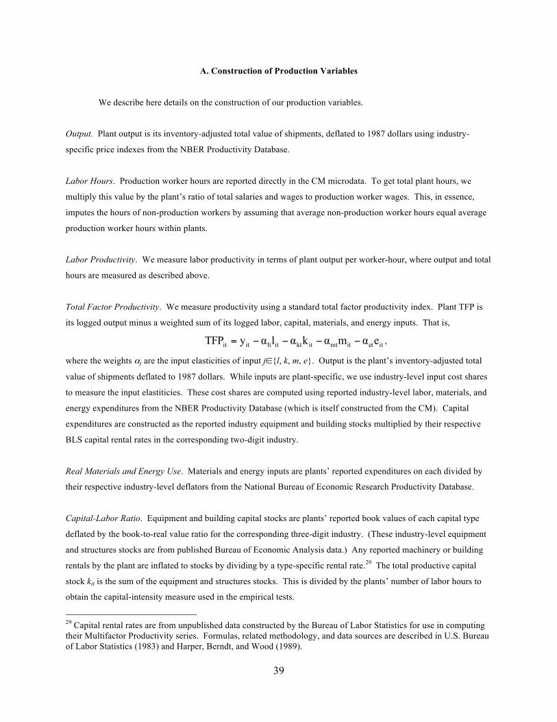
39

A. Construction of Production Variables

We describe here details on the construction of our production variables.

Output. Plant output is its inventory-adjusted total value of shipments, deflated to 1987 dollars using industry-

specific price indexes from the NBER Productivity Database.

Labor Hours. Production worker hours are reported directly in the CM microdata. To get total plant hours, we

multiply this value by the plant’s ratio of total salaries and wages to production worker wages. This, in essence,

imputes the hours of non-production workers by assuming that average non-production worker hours equal average

production worker hours within plants.

Labor Productivity. We measure labor productivity in terms of plant output per worker-hour, where output and total

hours are measured as described above.

Total Factor Productivity. We measure productivity using a standard total factor productivity index. Plant TFP is

its logged output minus a weighted sum of its logged labor, capital, materials, and energy inputs. That is,

itetitmtitktitltitit eαmαkαlαyTFP −−−−= ,

where the weights αj are the input elasticities of input j∈{l, k, m, e}. Output is the plant’s inventory-adjusted total

value of shipments deflated to 1987 dollars. While inputs are plant-specific, we use industry-level input cost shares

to measure the input elastiticies. These cost shares are computed using reported industry-level labor, materials, and

energy expenditures from the NBER Productivity Database (which is itself constructed from the CM). Capital

expenditures are constructed as the reported industry equipment and building stocks multiplied by their respective

BLS capital rental rates in the corresponding two-digit industry.

Real Materials and Energy Use. Materials and energy inputs are plants’ reported expenditures on each divided by

their respective industry-level deflators from the National Bureau of Economic Research Productivity Database.

Capital-Labor Ratio. Equipment and building capital stocks are plants’ reported book values of each capital type

deflated by the book-to-real value ratio for the corresponding three-digit industry. (These industry-level equipment

and structures stocks are from published Bureau of Economic Analysis data.) Any reported machinery or building

rentals by the plant are inflated to stocks by dividing by a type-specific rental rate.29 The total productive capital

stock kit is the sum of the equipment and structures stocks. This is divided by the plants’ number of labor hours to

obtain the capital-intensity measure used in the empirical tests.

29 Capital rental rates are from unpublished data constructed by the Bureau of Labor Statistics for use in computing their Multifactor Productivity series. Formulas, related methodology, and data sources are described in U.S. Bureau of Labor Statistics (1983) and Harper, Berndt, and Wood (1989).

40

Nonproduction Worker Ratio. Plants directly report both their number of production and nonproduction employees.

Nonproduction workers are defined by the Census Bureau as those engaged in “supervision above line-supervisor

level, sales (including a driver salesperson), sales delivery (truck drivers and helpers), advertising, credit, collection,

installation, and servicing of own products, clerical and routine office functions, executive, purchasing, finance,

legal, personnel (including cafeteria, etc.), professional and technical [employees]. Exclude proprietors and

partners.” The nonproduction worker ratio is simply such employees’ share of total plant employment.

B. Measuring the Flow of Goods through the Wholesale and Retail Sectors

The Input-Output Tables treat both the entire wholesale and retail sectors as single industries. Further, they

do not keep track of shipments by manufacturers to or through wholesalers or retailers, instead measuring only those

inputs directly used by wholesalers and retailers in the production of wholesale and retail services. To better

measure the flow of goods through these sectors, we the following algorithms.

If industry J is in the wholesale sector, we impute the industry’s purchases of each commodity C using CFS

data on establishments’ shipments of commodity C along with data from the Annual Wholesale Trade Survey

(AWTS). The AWTS contains information on wholesale industries’ aggregate commodity purchases and aggregate

commodity sales. Using data from the AWTS, we compute the ratio RJ of commodity purchases to sales.

Aggregating across plants in the CFS gives a measure of aggregate sales of each commodity by each wholesale

industry, SCJ. Given these two pieces of information, we impute industry J’s purchases of commodity C as PCJ =

SCJ·RJ.

To give an example, establishments in the motor-vehicle-related wholesale industries (SICs 5010-5019)

had sales of $159 billion and purchases of $131 billion in 1993. We therefore set RJ = 0.82 (131/159) for all

vehicle-related wholesale industries. For each commodity and industry within SICs 5010-5019, we impute

aggregate purchases as 82% of the shipments of the respective commodity that we observe CFS establishments

making.

When J is a retail industry, we utilize the CFS data along with the Annual Retail Trade Survey (ARTS).

The U.S. Census Bureau uses the ARTS to collect information on purchases of groups of retail industries. For

example, in 1993, establishments in the household appliance industries (SICs 5720-5734) purchased $35.8 billion in

intermediate materials. Unfortunately, we do not know how much total merchandise was purchased by each SIC

industry within these groupings, nor do we know the amount of any specific commodity purchased by these groups.

To impute these values, we rely on data from the Commodity Flow Survey and then hand match commodity-specific

shipments to the most appropriate retail industry within the ARTS groupings.

To demonstrate, we continue with our household appliance retailers example. Our hand match specifies

commodities 510102 (calculating and accounting machines), 510103 (electronic computers), 510104 (computer

peripheral equipment), and 510400 (other office machines) as those that are sold to SIC 5734 (computer and

41

software stores). Repeating this process for all commodities and industries yields a table of commodity-retail-

industry pairs such that the 4-digit retail industry could potentially purchase the given commodity.30 The amount of

the commodity purchased by the industry is assumed proportional to a) the amount of the good shipped, according to

the Commodity Flow Survey, b) the 4-digit retail industry’s share of employment among its larger grouping of

industries, and c) the total amount purchased by industry group.

For example, suppose we want to impute the purchases of computers (STCC 37531) by computer and

software stores. We know that total goods purchases by retailers in SICs 5720-5734 is $35.8 billion. Since

employment in computer and software stores is 14.6% (30,000/205,000) of employment in this retailer group, we

impute goods purchases of $5.2 billion by computer and software stores.31 To impute the amount of this total that is

computers specifically, we multiply the $5.2 billion figure by the value of shipments of computers as a fraction of all

commodities that can be purchased by computer and software stores, where both of these commodity values are

computed from the CFS.

C. Additional Robustness Checks

C.1. Plant-Level Shares of Internal Shipments

This section contains three additional robustness checks, related to those presented in Section IV.B.1. First,

we compute the distribution of internal shares using successively more restrictive definitions of vertically linked

industries. Then, we compare our measures of plants’ internal shares to the measures constructed directly from the

Census of Manufacturers. Finally, we discuss how our definitions of a) vertically linked industries and b) plants’

internal shipments differ from the definitions we gave in an earlier draft. We show that the results are robust to the

changes in our definitions.

In the benchmark calculations, we defined industry J to be downstream of industry I provided at least 1

percent of industry I’s sales were purchased by establishments in industry J. In Rows 1-3 of Table A1, we consider

the effect of changing the 1 percent cutoff to 10 percent, 15 percent, or 20 percent. As the cutoff increases two

things occur: First, our sample of upstream establishments shrinks. Second, for any particular establishment in our

sample, fewer shipments are classified as being sent along an internal, vertical link. Increasing the cutoff from 1 to

20 percent reduces the size of our sample by three-fifths. At the same time, however, the distribution of

establishments’ internal shares is not substantially altered using the more restrictive definition of vertical integration.

Under the 20 percent cutoff, the 75th(90th) percentile internal shares are 4.5 percent and 28.2 percent, only somewhat

smaller than the values given in Table 1.

30 The concordance of STCC commodities in the CFS and the commodity classifications in the Input-Output tables is produced in a two-step process. To match STCC commodities to the corresponding SIC industries, we use a table provided to us by John Fowler at the U.S. Census Bureau. To match SIC codes to IOIND commodities, we use the concordance provided by the BEA. The latter table can be found at http://www.bea.gov/industry/io_benchmark.htm. 31For these employment figures, see the “Establishment and Firm Size” document at http://www.census.gov/epcd/www/92result.html.

42

The Census of Manufacturers contains a variable, interplant transfers, which describes shipments that are

sent to other plants within the firm, for further assembly. Since the Census of Manufacturers also contains

information on each plant’s total value of shipments, it is straightforward to compute internal shares as the ratio of

interplant transfers to total value of shipments. The first row of Table A1 gives the quantiles for the 766 thousand

plant-year observations of plants’ interplant transfers. Only 2.2 percent of the observations have nonzero internal

shares. In the second row, we restrict attention to the 37,034 plants that also take part in the Commodity Flow

Survey. For this subsample, a larger fraction, 23.4 percent, have nonzero interplant transfers. The 90th percentile

interplant transfers share is 13.2 percent.

Rows 3 and 4 of Table A1 give the corresponding statistics, using our benchmark definitions of plants’

internal shares (i.e., using data from the Commodity Flow Survey and the algorithm specified in Section 3 of the

paper). Row 3 restricts the benchmark sample to plants in the manufacturing sector. For this subsample, the 75th

(90th) percentile internal share is 6.2 percent (33.7 percent), slightly lower than the values given in Table 1 (7.0

percent, and 37.6 percent, respectively).

The difference between Rows 5 and 6 originates from differences in what is defined as an internal

shipment. Interplant transfers, which are shipments to other plants for further assembly, only includes shipments

sent to plants in the manufacturing sector. Our definition, using data from the Commodity Flow Survey, includes

shipments sent to same-firm plants in any sector.

In Row 4, we only count a shipment as internal if there is a downstream plant, from the same firm, that is

also in the manufacturing sector. 32 The 75th(90th) percentile internal shares are 0.3 percent and 11.7 percent,

reasonably close to the values given in Row 5.

To summarize, the interplant transfers variable yields smaller values for internal shipments, compared to

the variable constructed from the Commodity Flow Survey, because it omits shipments sent to non-manufacturing

establishments. If it were not for this difference, the two variables would be similar to one another.

Our definitions over which industries are vertically linked and when shipments are counted as internal were

slightly different in an earlier draft of the paper (Hortacsu and Syverson, 2007b). It turns out that results are

qualitatively similar whether one uses the old or new definitions of vertically linked industries or internal shipments.

For completeness, we review these old definitions, as well as the internal shares that resulted from these definitions.

In the previous draft, we had a less stringent definition for internal shipments. We did not require that the

shipment be destined to an establishment that is in an industry directly downstream to the shipping establishment,

only that the destination be a plant that is on the downstream end of any vertical link in a firm.33 In Row 8 of Table

A1, we recomputed internal shares for the benchmark sample, with this less strict definition of internal shipments.

32 Consider the following example of a plant, sending a shipment of auto parts to zip code, z. Suppose there is a same-firm auto parts wholesaler (SIC=5013), but no manufacturing plants in an industry that consumes auto parts, in zip code z. This shipment would be classified as internal according to the calculations of Row 3, but in not the calculations corresponding to Row 4. 33 For instance, suppose a firm has two upstream establishments U1 and U2, and two downstream establishments D1 and D2, and U1-D1and U2-D2 are separate vertical links. According to the old definitions, a shipment from U1 would be classified as internal if it is destined to either D1 or D2’s ZIP codes, not just D1’s.

43

The median plant has an internal share of 3.0 percent, and only 29.1 percent of plants have no internal shipments.

Compared to the benchmark calculations, the mean internal share is almost 6 percent larger (16.1 percent, compared

to 10.2 percent). Thus, under our old definitions, we were being very liberal when computing internal shipments.34

A second difference, compared to the previous draft, originates from the way in which vertically linked

industries are defined. In the previous draft, we defined two industries to be vertically linked only using information

from the BEA input-output tables. Specifically, a substantial link exists between Industry A (using the BEA

definition of input-output industries) and any industry from which A buys at least five percent of its intermediate

materials, or any industry to which A sells at least five percent of its own output. As we discuss in Section 3, the old

definition is potentially problematic if the downstream industry is retail or wholesale. For wholesalers and retailers,

the BEA doesn't keep track of the gross shipments by sent to wholesalers/retailers. Instead, the BEA measures the

industries which are used by wholesalers/retailers in the "production" of wholesale/retail services. Because of this

issue, there are several pairs of industries that are, in reality, linked with one another, but are not classified as such

under the old definition.

In Row 9 of Table A1, we compute internal shares using the old definition of vertically linked industries

(but retain the new definition of when shipments are internal to the firm). With the old definition of vertically linked

industries, the sample of vertically integrated establishments is less than half as large, 29893 compared to 67552

plant-years. The 75th percentile (90th percentile) internal share is 1.0 percent (17.4 percent). These are considerably

less than corresponding values of the benchmark calculations for the 75th and 90th percentiles, 7.0 percent and 37.6

percent.

In the final row, Row 10, of Table A1, we compute internal shares using both the old definition of when

shipments are classified as internal, and the old definition of when industries are classified as vertically linked.

Under these definitions, the median establishment has an internal share of 2.5 percent, the 90th percentile plant has

an internal share of 57.7 percent, and 2.1percent of plants have a 100 percent internal share.

C.2. Is Geographic Closeness Important?

It’s quite likely that some of the low internal shares we see above arise because a firm’s plants are too

spatially separated to make internal shipments practical. Of course, if this is the case, this may be a result as much a

cause of the lack of within-firm goods transfers along a production chain. If moving physical products down a

production chain was the only reason for vertical ownership, after all, no firm would own vertically related plants

that were located too far from one another to make intra-firm shipments impractical. The fact that firms do own

vertically linked producers that are far apart suggests other motives for ownership.35

34 Since a main objective of the paper is to point out that internal shipments are surprisingly small, being liberal in defining internal shipments is innocuous. 35 Hortaçsu and Syverson (2007) document examples of vertically integrated cement and concrete firms that own clusters of ready-mixed concrete plants that are remotely located from their upstream cement plants. These firms, in fact, do not internally supply these clusters with cement. The downstream concrete plants report instead buying cement in the local market from the firm’s upstream competitors. We find evidence that the firms’ motives for owning these concrete plant clusters is to harness logistical efficiencies in a business that shares a common final demand sector (construction) with cement.

44

Nevertheless, it is interesting to quantify how much distance matters. We take two approaches. The first is

to compute the distribution of internal shipment shares for firms whose plants are all located close to one another.

The second is to compare plants’ shipment distances to the distances they are from other plants in their firms.

To see shipment patterns of closely-spaced firms, we use the subset of upstream plants from our CFS

sample where all of the plants that their firm owns are in the same county. (This is determined from the Economic

Census, which includes state and county codes for virtually all establishments. This location information is not

subject to the limitations of the EC zip code data, where codes for 10 percent of plants are missing.) This subset is

small—2254 plant-years and 199,712 shipments—and contains a large number of two-plant firms with one upstream

and downstream plant each. Nevertheless, it offers a rough gauge the role of distance.

The results are consistent with the patterns above. Just under half (46.7 percent) of the upstream plants

report no shipments to downstream units in their firm. The 90th percentile plant ships 49.0 percent of the value of its

shipments internally. The fraction of plants with all shipments staying in the firm is above that in the benchmark

sample, however, at 2.4 percent. Thus it appears that vertically structured firms with closely located plants are less

likely to make internal shipments on average, but somewhat more likely to contain internally dedicated upstream

plants.

We next compare the shipment distances of our entire sample of upstream plants in the CFS to their

distances from other plants in their firms (both measured in great circle terms). It’s clear from pooling shipments

across plants that internal shipments go shorter distances. In fact, the average external shipment is sent roughly

three times as far as the average internal shipment. This may reflect upstream plants “bypassing” their downstream

units with some of their shipments, but it may also reflect composition effects if internally dedicated, high-volume

upstream establishments are located close to downstream units in their firm.

We can decompose these contributions to the pooled numbers by looking within plants. We find that for

21.9 percent of upstream shipment plants, their farthest-traveling shipment does not go as far as the distance to the

nearest downstream plant in their firm. These plants account for just under one-third of the one-half of our upstream

plants that report no internal shipments, showing the importance of distance. But this also means the other two-

thirds of plants reporting no internal shipments do send output at least as far as their nearest plant. This pattern isn’t

unusual across the broader sample. Looking across plants, the average of the within-plant medians of reported

shipment distances is 274 miles, while the average distance to the closest downstream plant within the firm is 192

miles.

C.3. Is There Vertical Integration Within Plants?

Our definition of vertically integrated ownership links requires multiple plants by definition. A firm must

own at least one plant each in vertically related upstream and downstream industries. This definition could be

problematic if firms commonly vertically integrate production within a single plant. In such cases, the firm would

be operating a vertically integrated production process and obviously supplying its own input needs. We would

miss this type of integration, however, because we would not classify the plant as integrated. There would be no

shipments from the upstream to downstream parts of the production process in the CFS, since those goods transfers

45

never leave the plant.

To give a concrete example, consider the two following hypothetical firms. One has two plants. The

upstream plant refines copper ore into billets which are then shipped to the downstream plant to be extruded into

pipe. The second firm operates a similar production process in a single plant: one side refines ore into billets, and

the other side turns billets into pipe. We would define the former plants as vertically integrated, but not the latter,

even though each firm operates the same production processes.

How can we tell if this sort of misclassification is a big problem? We compare the materials purchase

patterns of plants that we classify as being in vertical structures to those in the same industry not classified as such.

In the context of the above example, we compare the two copper pipe plants. (Since plants are classified into

industries in the Economic Census based upon their outputs, both the downstream plant in the first firm and the

second firm’s plant would be classified in the same industry, SIC 3351: Rolling, Drawing, and Extruding of

Copper.) The pipe plant in the first firm—the one that we would have classified as in a vertical ownership

structure—will list copper billets as an intermediate materials purchase in the Census of Manufactures materials

supplement. The second plant, where billet production is inside the plant, will list copper ore as a materials

purchase. Hence if we see substantial differences in materials use patterns across plants (in the same industry) that

we classify respectively as vertically linked or not, we should be concerned that we are missing a lot of vertical

production that occurs “under one roof.” On the other hand, a lack of significant differences suggests this sort of

misclassification is less of a concern.

We make three such comparisons between the materials use patterns of what we classify as vertically

linked plants and others in their industry. (Again our analysis is restricted to plants in the manufacturing sector

because of the detailed intermediate materials data requirements.) We first compute the share of each plant’s

intermediate materials purchases that is for “raw materials,” which we define as the products of the agricultural,

fisheries, forestry, or mining sectors—i.e., SIC product codes beginning with “14” or below. We then regress this

share on a set of industry-year fixed effects and an indicator equal to one if we classify the plant as in a vertical

ownership link. In essence, we test whether there are significant differences in the intensity of raw materials use

across plants that we classify as vertical and non-vertical in the same industry. We would expect that if the “under

one roof” misclassification problem were substantial, we would find that plants we designate as non-vertical would

have a larger raw materials share, since a greater portion of the production chain would be operated within the plant.

Again, to return to our example, the pipe plant in the second firm reports copper ore (a raw material) as a materials

purchase, while the plant in the first firm purchases copper billets.

We run this regression on a sample of over 453 thousand plant-years from the Census of Manufactures.

(We don’t need the CFS for this.) The coefficient on the vertical ownership link indicator is 0.47 percent, with a

standard error of 0.05 percent. Thus plants we classify as vertical use raw materials more, not less, intensively

compared to other plants in their industry. (Recall that we would expect plants we classify as vertically linked to use

raw materials less intensively). Further, the point estimate of the share difference is small, less than one-fifteenth

the average raw materials share of 8.2 percent. Even if we restrict our comparisons only to those roughly 85,000

plants that report using positive raw materials shares, the vertically linked coefficient is -1.87 percent with a 0.19

46

percent standard error. The estimated difference is small, relative to the 44 percent average materials share, for

plants that report positive materials purchases.

Our second check aggregates this raw materials use data to the industry level. We add up raw and total

materials use of plants classified as vertical within an industry year, and compare the ratio of the two to the same

share computed for non-vertical (again, under our classification) plants in the same industry. We then conduct a t-

test for equality of means across our sample of 1867 industry-years. The mean difference is 0.08 percent, with a

standard error of 0.22 percent. Here, there are no significant within-industry differences in raw materials usage

intensity across the two types of plants.

Our final check is also done at the industry-year level. We separately aggregate materials purchases of our

designated vertical and non-vertical plants for each industry year. We then order materials by decreasing intensity

of use for each type of plant (as measured by their aggregate share of purchases). This yields 86,659 industry-year-

materials ranks for both vertical and non-vertical plants. We then compare these ranks within industry-year to see if

there are systematic differences. The two ranks move together; the correlation coefficient is 0.74. Table A2 shows

the frequency of relative rank orderings for the five most intensively used materials by industries’ non-vertical

plants. (Material 1 is the most intensively used.) Only ranks 1-7 of vertical plants are shown for parsimony. If

materials usage patterns were exactly the same, we would only see entries on the diagonal of the table. The most

intensively used material of an industry’s vertical plants would be the most intensively used among its non-vertical

plants; the second-most used would be so for both types of plants, and so on. Clearly, this is not the case. However,

the general pattern holds. The diagonal is the largest element of a row or column, and the frequency of other

pairings falls as they move further away from the diagonal. Hence these results suggest, as do the raw materials use

tests above, that there are not systematic differences in the mix of materials used by plants we classify as in vertical

ownership links and those we do not classify as such.

C.4. Cross-Industry Differences in Internal Shares

Table A3 presents, for different 2 and 3-digit industries, establishments’ average internal shares. The first

three columns use data from the Commodity Flow Survey, while the final three columns use data from the Census of

Manufacturers.

The first column gives, for all establishments surveyed in the Commodity Flow Survey, the fraction of

plants that have a positive internal share. There is substantial variation, across different goods-producing industries.

Plants in petroleum and transportation equipment manufacturing have the largest fraction of plants within positive

internal shares; furniture manufacturers and furniture and lumber wholesalers have the smallest fraction of plants

with positive internal shares. The second and third columns give the revenue-weighted average share of plants’

internal shares. Again, there is substantial variation, among industries with the highest average internal shares

(fabric and petroleum manufacturing, and chemicals and beer/wine wholesaling) and the industries with the lowest

average internal shares (furniture manufacturing and lumber, metals, drugs, and petroleum wholesaling.

Columns 4-6 display the corresponding calculations, using data from the Census of Manufacturers. While

both the sample and the definition of internal shares differ between columns 1-3 and columns 4-6, the cross-industry

47

patterns of internal shares are similar across the two sets of calculations. Paper, transportation equipment, and

primary metals manufacturing are some of the more vertically integrated industries; furniture manufacturing and

printing are two of the least vertically integrated.

The petroleum industry is a bit of an outlier, and deserves extra attention. Petroleum is an industry that has

one of the highest internal shares in columns 1-3, but one of the lowest internal shares in columns 4-6. This

difference results from the different definitions of internal shipments across the two datasets. The Interplant

Transfers variable, collected in the Census of Manufacturers, asks plants to give the value of shipments sent to other

manufacturing plants for further assembly. Since shipments by petroleum manufacturers are mainly sent to

wholesalers, and not to other manufacturers, the internal shares computed from the Census of Manufacturers tend to

be significantly smaller than the internal shares computed using data from the Commodity Flow Survey.

C.5. Firm Size Differences by Firm Structure

Figure A1 plots the densities of firm size (logged total employment, since revenue is unavailable outside of

manufacturing) for three mutually exclusive and exhaustive sets of multi-establishment firms. One set includes

firms with vertical ownership structures.36 The other two multi-unit organizational structures are single-industry and

multi-industry-unintegrated firms.37

The figure reveals that each of the (logged) employment size distributions is unimodal, though they clearly

have different central tendencies.38 Single-industry multi-unit firms are the smallest and have the most symmetric

size distribution. Vertically integrated firms are clearly the largest on average, and their distribution is more skewed

than the other firm types. (While not plotted, single-establishment firms are smaller than the multi-unit single-

industry firms, as one might expect.) Thus not only are vertically integrated plants larger, their firms are as well.

C.6. Flows of Intangible Inputs

In our product mix and shipment destination tests, we use the following algorithm to identify plants that

experienced ownership changes. From the Longitudinal Business Database, we begin with all establishments for

which the firm identifier changes between t and t+1. Since firm identifiers may change across years for a number of

reasons, we need to discard the observations which are unrelated to mergers or acquisitions.39 To identify actual

36 Recall that we define vertical ownership at the plant, not firm level. For our purposes here, however, we define a firm as vertically structured if it owns any vertically linked establishments. As a practical matter, most plants in what we call vertically structured firms here are also in vertical chains according to our plant-specific definition. 37 The distribution of plants across these firm sets is as follows. Over the entire manufacturing sample, multi-unit plants of all types accounted for 19.7 percent of establishments, 71.8 percent of employment, and 86.5 percent of the capital stock. Vertically integrated plants’ shares were, respectively, 14.3, 60.1, and 79.1 percent. Multi-unit single-industry plants accounted for 2.8 percent of establishments and 5.1 and 3.2 percent of employment and capital, while multi-industry unintegrated plants comprised 3.9, 8.3, and 5.5 percent of establishments, employment, and capital. 38 We only plot the 1997 distributions rather than those pooled across years in order to remove any secular shifts in firm sizes. Checks of other years show similarly shaped distributions. 39 For example, legal reorganizations may cause a change in firm identifiers without an actual change in ownership. For an additional example, multi-unit and single-unit firms are coded differently by the Census: a single-unit

48

changes in ownership, we consider the set of establishments that have the same firm identifier as that establishment

in years t and t+1. For these establishments, we say that a change of ownership has occurred if they share the same

firm identifier with some other set of establishments in period t+1, but not in period t. We define the other set of

establishments to be an acquiring firm, if their firm identifier is the same in both years t and t+1.40

Here, we complement our analysis in the main text of summary data on changes in product mix and

shipment destinations among acquired plants with more formal analyses. In Table A4, we estimate the probability

that plant i will produce a given 7-digit product in year t as a function of the year t-5 production patterns of the

acquiring and acquired firms. We find a plant is more likely to produce a product in year t if either the acquiring or

the acquired firm was producing the product. The probability that an acquired plant produces a given 7-digit

product in year t is 6 percent higher for products that were produced by the acquiring firm in year t-5. Compared to

other products in their industry, acquired establishments are also more likely to produce the products that its original

firm was producing. The probability that establishment i produces a given 7-digit product is 7 percent higher for

products that were produced in year t-5 by some other establishments of the acquired firm.

To further explore the evolution of acquired establishments’ shipping patterns, we run a series of logit

regressions to estimate the probability that an acquired plant i will ship to any particular zip code z in 1997. In these

regressions, the variables of interest measure the shipping patterns of the acquiring and acquired firms in 1993. In

addition, we include the following variables as controls: establishment-by-destination-county fixed effects; controls

for total sales to zip code z as well as the great-circle distance between i and z, an indicator variable equal to one if

there exists an establishment from the same firm in 1997, and an indicator variable equal to one if establishment i

shipped to z in 1993.

Table A5 contains the results from these regressions. An establishment is significantly more likely to ship

to a zip code if either the acquiring or acquired firm sold to that zip code in previous years. The probability that

plant i sells to zip code z in 1997 is 1.2 percent higher when an establishment from the acquiring firm sold to that zip

code in 1993. The estimated marginal effect is significantly larger, 9.6 percent, if the establishment from the

acquiring firm shares the same 4-digit industry as the acquired establishment. Finally, these marginal effects are

economically meaningful. The average probability that an acquired establishment in our sample sells to a particular

zip code is 4.0 percent. Furthermore, the acquired plant i is more likely to ship to the zip codes that it used to sell to,

and to the zip codes that other plants in the acquired firm were selling to.

We also estimate these logit regressions with different subsets of the sample of acquired establishments. In

establishment that opens a new establishment elsewhere will have its firm identifier change, again without any change in ownership. 40 An example will help explain how the algorithm works. Consider a two-establishment firm with establishment identifiers I1 and I2, and firm identifier F in year t, and firm identifier G in year t+1. If there are no other establishments in year t+1 that have firm identifier G, then the algorithm would not identify a change of ownership. On the other hand, if there exists some establishment, I3 that had firm identifier G in year t, our algorithm would identify I3 as the sole establishment in the acquiring firm; I1 and I2 would then be classified as members of the acquired firm. Using a different method, Nguyen (1998) constructs a sample of acquired establishments, called the Ownership Change Database. As a robustness check, we re-create Tables A5 and A6 using the Ownership Change Database. The results are presented in the final columns of Tables A6 and A7.

49

Table A6, we re-estimate the probability than a plant manufacturers a given 7-digit product. Again, we cut the data

according to the year of the acquisition (column 1 versus column 2). We also run the logit regression separately for

plants that were in multi-unit firms and single-unit firms (column 3 versus column 4). Finally, we use a dataset—the

Ownership Change Database constructed by Sang V. Nguyen of the Census Bureau, as the source of acquired

establishments. Coefficient estimates are similar across the different subsamples. In particular, in each

specification, the probability that plant i manufactures a particular 7-digit product is at least 5.5 percent larger when

the acquiring firm had a plant that, in year t-5, produced that same product.

Table A7 presents robustness checks related to the estimation of the probability that an acquired

establishment ships to a particular zip code. In the first two columns, we show that the estimated effects are similar

for plants that merge earlier or later on. In the third and fourth columns, we show that the estimated effects are

similar for establishments that were, in 1992, part of a multi-unit or a single-unit firm.41 In the fifth column, we

estimate the probability of shipping to a particular zip code for plants in the wholesale, instead of the manufacturing,

sector. For wholesalers, the coefficient on the indicator that another establishment in the same 2- (or 4-) digit SIC

sells to z in 1993 is statistically indistinguishable from 0. Finally, in the sixth column, there is no substantial

difference in the estimated effects from using the Ownership Change Database to define the set of acquired

establishments.

41 Since, in the fourth column, the sample includes only establishments that are in single-unit firms in 1992, the I(in 1993, another establishment, from the acquired firm, shipped to z) indicator is 0 for all plants. Thus, this variable is excluded from the list of independent variables.

Table A1. Plant-Level Shares of Internal Shipments: Additional Robustness Checks

Percentile

Specification/Sample 25th 50th 75th 90th 95th Frac. = 0 Frac. = 1 Approx. Plant-years

1. 10% cutoff definition for VI 0.0% 0.0% 4.4% 28.7% 58.8% 55.1% 0.8% 43,000

2. 15% cutoff definition for VI 0.0% 0.0% 4.3% 27.3% 55.3% 55.0% 0.7% 34,000

3. 20% cutoff definition for VI 0.0% 0.0% 4.5% 28.2% 55.1% 55.1% 0.7% 27,000

4. Interplant transfers 0.0% 0.0% 0.0% 0.0% 0.0% 97.8% 0.1% 766,000

5. Interplant transfers, plants surveyed in CFS 0.0% 0.0% 0.0% 13.2% 51.1% 76.6% 1.1% 37,000

6. Plants that are in the CMF 0.0% 0.0% 6.2% 33.7% 64.5% 50.9% 1.1% 37,000

7. Plants that are in the CFM, shipments to manufacturers 0.0% 0.0% 0.3% 11.7% 33.5% 71.1% 1.1% 37,000

8. Don’t require the sending and receiving establishments to be part of a vertical link

0.0% 3.0% 19.4% 59.2% 84.8% 29.1% 2.1% 68,000

9. Original method for defining vertical links 0.0% 0.0% 1.0% 17.4% 44.5% 67.5% 0.8% 30,000

10. Original method for defining vertical links & Don’t require the sending and receiving establishments to be part of a vertical link.

0.0% 2.5% 18.9% 57.7% 84.0% 33.7% 2.1% 30,000

Notes: Each row shows for a different subsample the distributions of the shares (by dollar value) of upstream integrated establishments’ shipments that are internal to the firm. The criteria for inclusion in and size of each subsample is discussed in the text. For data confidentiality reasons, the reported percentiles are averages of immediately surrounding percentiles; e.g., the median = 0.5*(49th percentile + 51st percentile).

Table A2. Relative Material Use Intensity Ranks between Plants in Vertical Ownership Structures and Other Plants

Material’s intensity rank in non-vertically linked plants 1 2 3 4 5

Material’s intensity rank in vertically linked

plants

1 50.5% 13.7% 8.0% 4.5% 3.3% 2 14.7% 26.1% 15.4% 10.1% 6.0% 3 8.1% 14.7% 19.1% 13.2% 9.8% 4 5.6% 10.6% 12.1% 14.8% 11.8% 5 3.1% 6.5% 9.6% 11.2% 11.3% 6 3.2% 5.1% 6.5% 7.9% 10.4% 7 2.2% 4.3% 5.9% 6.4% 7.3%

Notes: This table shows, for a sample of 9545 industry-material-year cells, the ranks of materials intensity use (by share of materials purchases) for the five most intensively used materials in plants we define as not in vertical ownership structures. The entries in the table correspond to the fraction of cells where vertical and non-vertical plants in the same industry share a particular pair of materials intensity rankings. For example, across all industry-years in the sample, the most intensively used (rank 1) material by non-vertical plants in an industry-year is the most intensively used material by the industry-year’s vertical plants 50.5 percent of the time. Non-vertical plants’ rank 1 material is vertical plants’ second most intensively used material 14.7 percent of the time, and so on.

Table A3. Plant-Level Shares of Internal Shipments, by Industry

Using Commodity Flow Survey Data Using Census of Manufacturers Data

Industry Fraction of plants w/ share > 0

Mean share Mean share,

cond. on share > 0

Fraction of plants w/ share > 0

Mean share Mean share,

cond. on share > 0

12, Coal Mining 26.0% 10.6% 40.8%

14, Stone 27.7% 6.6% 23.7%

20, Food 52.4% 11.0% 20.9% 3.7% 3.5% 13.9%

22, Fabric 50.5% 17.4% 34.4% 8.3% 20.5% 53.1%

23, Apparel 32.9% 6.6% 19.9% 0.8% 4.3% 46.4%

24, Wood 31.1% 6.1% 19.5% 1.4% 4.7% 27.3%

25, Furniture 16.1% 1.6% 10.2% 0.9% 0.9% 10.1%

26, Paper 40.4% 5.6% 13.9% 11.1% 10.0% 25.1%

27, Printing 21.6% 2.4% 11.2% 0.3% 0.6% 16.7%

28, Chemicals 49.2% 8.3% 16.9% 6.4% 7.5% 19.4%

29, Petroleum 76.8% 28.8% 37.5% 8.8% 3.0% 6.8%

30, Plastics 28.0% 4.4% 15.8% 4.0% 3.4% 18.0%

31, Leather 38.0% 11.2% 29.6% 1.3% 3.7% 31.3%

32, Glass, Stone 38.5% 6.1% 15.9% 1.5% 4.0% 25.0%

33, Primary Metals 48.9% 8.4% 17.2% 7.6% 11.0% 26.1%

34, Fabr.Metals 26.7% 5.4% 20.3% 2.1% 6.1% 34.2%

35, Ind. Machinery 40.8% 4.8% 11.9% 1.3% 4.4% 18.8%

36, Elc. Equipment 46.4% 7.1% 15.3% 3.5% 6.5% 26.3%

37, Trans. Equip. 65.6% 11.2% 17.2% 4.5% 9.4% 28.6%

38, Instruments 43.8% 6.7% 15.4% 2.2% 3.3% 11.4%

39, Miscellaneous 11.9% 2.2% 18.4% 0.5% 1.1% 13.3%

501, Vehicles 52.7% 6.7% 12.7%

502, Furniture 17.5% 2.2% 12.5%

503, Lumber 17.9% 1.5% 8.4%

504, Prof. Equip. 31.4% 5.1% 16.1%

505, Metals 24.3% 2.0% 8.4%

506, Electrical 34.4% 3.5% 10.0%

507, Hardware 25.3% 2.8% 10.9%

508, Machinery 29.1% 2.9% 10.0%

509, Miscellaneous 8.7% 1.1% 13.1%

511, Paper 34.8% 2.5% 7.2%

512, Drugs 26.5% 1.3% 5.0%

513, Apparel 27.6% 3.5% 12.8%

514, Groceries 32.3% 6.8% 21.0%

516, Chemicals 33.1% 12.6% 38.0%

517, Petroleum 20.4% 1.8% 8.8%

518, Beer & Wine 52.9% 17.2% 32.5%

519, Miscellaneous 11.1% 1.2% 11.0%

Note: Each row shows, for a different SIC industry, the fraction of plants that have positive internal shipments, as well as the average share of internal shipments. Industries in the mining and manufacturing sectors are averaged over 2-digit industries. Industries in the wholesale sector are averaged over 3-digit industries.

Table A4. Logit Regression: Probability Plant i Produces a Given 7-digit Product in Year t

I(estab. produced 6-digit product in t-5) 1.215* (0.037) 0.086

0.921* (0.038) 0.052

1.058* (0.039) 0.063

I(estab. produced 7-digit product in t-5) 2.366* (0.036) 0.422

2.189* (0.037) 0.400

2.189* (0.037) 0.399

I(in t-5, another estab. from the acquired firm produced the 6-digit product)  

0.321* (0.059) 0.018

0.321* (0.059) 0.018

I(in t-5, an estab. from the acquiring firm produced the 6-digit product)  

0.113* (0.054) 0.006

0.113* (0.054) 0.006

I(in t-5, another estab. from the acquired firm produced the 7-digit product)

0.608* (0.054) 0.052

I(in t-5, an estab. from the acquiring firm produced the 7-digit product)

0.702* (0.051) 0.053

Approx. N 140,000 140,000 140,000 Approx. number of establishment-by-4-digit industry groups 7,600 7,600 7,600

Pseudo R2 0.353 0.363 0.368 Average probability that i produces the 7-digit good in year t 13.1% 13.1% 13.1%

Notes: Each column gives the results from a separate logit regression. The dependent variable equals 1 provided plant i produces 7-digit product, p, in year t. The sample includes all i-p pairs for which a) i was purchased between t-5 and t-1, and b) product p was produced at least such acquired plant in year t. Controls for total sales in year t of the 7-digit product (minus sales of the product by plant i) are included, but not reported. t ∈ {1987, 1992}. All regressions include establishment-by-4-digit-product fixed effects. An asterisk denotes significance at a five percent level.

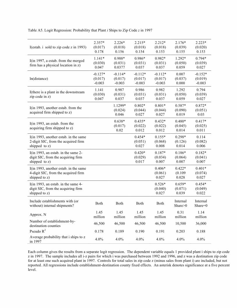
Table A5. Logit Regression: Probability that Plant i Ships to Zip Code z in 1997

Each column gives the results from a separate logit regression. The dependent variable equals 1 provided plant i ships to zip code z in 1997. The sample includes all i-z pairs for which i was purchased between 1992 and 1996, and z was a destination zip code for at least one such acquired plant in 1997. Controls for total sales in zip code z (minus sales from plant i) are included, but not reported. All regressions include establishment-destination county fixed effects. An asterisk denotes significance at a five percent level.

I(estab. i sold to zip code z in 1993) 2.357* (0.017) 0.178

2.226* (0.018) 0.156

2.215* (0.018) 0.154

2.212* (0.018) 0.153

2.176* (0.039) 0.155

2.223* (0.020) 0.153

I(in 1997, a estab. from the merged firm has a physical location in z)

1.141* (0.030) 0.047

0.988* (0.031) 0.0377

0.986* (0.031) 0.037

0.982* (0.031) 0.037

1.292* (0.050) 0.059

0.794* (0.039) 0.027

ln(distance) -0.127* (0.017) -0.003

-0.114* (0.017) -0.003

-0.112* (0.017) -0.003

-0.112* (0.017) -0.003

0.007 (0.037) 0.000

-0.152* (0.019) -0.003

I(there is a plant in the downstream zip code in z)

1.141 (0.030) 0.047

0.987 (0.031) 0.037

0.986 (0.031) 0.037

0.982 (0.031) 0.037

1.292 (0.050) 0.059

0.794 (0.039) 0.027

I(in 1993, another estab. from the acquired firm shipped to z)

1.1299* (0.024) 0.046

0.802* (0.044) 0.027

0.801* (0.044) 0.027

0.587* (0.090) 0.019

0.872* (0.051)

0.03

I(in 1993, an estab. from the acquiring firm shipped to z)

0.638* (0.017)

0.02

0.435* (0.022) 0.012

0.432* (0.022) 0.012

0.480* (0.045) 0.014

0.417* (0.025) 0.011

I(in 1993, another estab. in the same 2-digit SIC, from the acquired firm shipped to z)  

0.454* (0.051) 0.027

0.155* (0.068) 0.008

0.298* (0.126) 0.014

0.114 (0.082) 0.006

I(in 1993, an estab. in the same 2-digit SIC, from the acquiring firm shipped to z)  

0.420* (0.029) 0.017

0.187* (0.034) 0.007

0.186* (0.064) 0.007

0.182* (0.041) 0.007

I(in 1993, another estab. in the same 4-digit SIC, from the acquired firm shipped to z)

0.406* (0.061) 0.027

0.422* (0.109 0.028

0.401* (0.074) 0.027

I(in 1993, an estab. in the same 4-digit SIC, from the acquiring firm shipped to z)

0.526* (0.040) 0.027

0.659* (0.071) 0.039

0.454* (0.049) 0.022

Include establishments with (or without) internal shipments? Both Both Both Both Internal

Share>0 Internal Share=0

Approx. N 1.45 million

1.45 million

1.45 million

1.45 million

0.31 million

1.14 million

Number of establishment-by-destination counties 46,500 46,500 46,500 46,500 10,500 36,000

Pseudo R2 0.178 0.189 0.190 0.191 0.203 0.188 Average probability that i ships to z in 1997 4.0% 4.0% 4.0% 4.0% 4.0% 4.0%

Table A6. Logit Regression: Probability Plant i Produces a Given 7-digit Product in Year t; Robustness Checks

I(estab. produced 6-digit product in t-5) 1.086* (0.051) 0.070

1.022* (0.061) 0.060

1.066* (0.042) 0.064

1.009* (0.103) 0.064

1.046* (0.034) 0.057

I(estab. produced 7-digit product in t-5) 2.093* (0.049) 0.391

2.326* (0.058) 0.427

2.181* (0.040) 0.399

2.241* (0.101) 0.418

2.379* (0.032) 0.427

I(in t-5, another estab. from the acquired firm produced the 6-digit product)

0.306* (0.074) 0.018

0.336* (0.097) 0.019

0.317* (0.059) 0.018

0.343* (0.051) 0.018

I(in t-5, an estab. from the acquiring firm produced the 6-digit product)

-0.054 (0.072) -0.003

0.343* (0.083) 0.020

0.090 (0.058) 0.005

0.224 (0.142) 0.013

0.065 (0.058) 0.003

I(in t-5, another estab. from the acquired firm produced the 7-digit product)

0.599* (0.069) 0.053

0.631* (0.087) 0.056

0.612* (0.055) 0.052

0.644* (0.047) 0.052

I(in t-5, an estab. from the acquiring firm produced the 7-digit product)

0.752* (0.068) 0.054

0.651* (0.077) 0.056

0.675* (0.055) 0.050

0.879* (0.139) 0.073

0.787* (0.055) 0.055

Year of merger t-5 to t-3 t-2 to t-1 t-5 to t-1 t-5 to t-1 t-5 to t-1 Multi-unit/single unit in t-5? Either Either Multi Single Either Use Ownership Change Database to define mergers? No No No No Yes

Approx. N 83,000 57,000 119,000 21,000 215,000 Approx. number of establishment-by-4-digit-industry groups 4,700 2,900 6,600 1,000 10,600

Pseudo R2 0.353 0.391 0.375 0.322 0.385 Average probability that i produces the 7-digit good in t 13.2% 13.0% 13.3% 11.8% 11.8%

Notes: Each column gives the results from a separate logit regression. The dependent variable equals 1 provided plant i produces 7-digit product, p, in year t. The sample includes all i-p pairs for which a) i was purchased between t-5 and t-1, and b) product p was produced at least such acquired plant in year t. Controls for total sales in year t of the 7-digit product (minus sales of the product by plant i) are included, but not reported. See text for details. t {1987, 1992}. All regressions include establishment-4-digit product fixed effects. An asterisk denotes significance at a five percent level.

Table A7. Logit Regressions: Probability Plant i Ships to Zip Code z in 1997. Robustness Checks

Notes: Each column gives the results from a separate logit regression. The dependent variable equals 1 provided plant i ships to zip code z in 1997. The sample includes all i-z pairs for which i was purchased between 1992 and 1996, and z was a destination zip code for at least one such acquired plant in 1997. Controls for total sales in zip code z (minus sales from plant i) are included but not reported. All regressions include establishment-destination-county fixed effects. An asterisk denotes significance at a five percent level.

I(Estab. i sold to zip code z in 1993) 2.184* (0.023) 0.155

2.249* (0.027) 0.152

2.201* (0.019) 0.151

2.304* (0.057) 0.146

1.489* (0.027) 0.132

2.263* (0.015) 0.174

I(in 1997, an estab. from the merged firm has a physical location in z)

0.547* (0.005) 0.013

0.526* (0.006) 0.012

1.003* (0.031) 0.038

0.600* (0.142) 0.016

1.192* (0.055) 0.095

0.991* (0.030) 0.041

ln(distance) -0.100* (0.022) -0.002

-0.126* (0.026) -0.003

-0.100* (0.018) -0.002

-0.228* (0.052) -0.004

-0.104* (0.021) -0.005

-0.096* (0.015) -0.002

I(in 1993, another estab. from the acquired firm shipped to z)

0.842* (0.058) 0.030

0.746* (0.068) 0.024

0.805* (0.044) 0.027

0.777* (0.124) 0.051

0.558* (0.037) 0.018

I(in 1993, an estab. from the acquiring firm shipped to z)

0.458* (0.030) 0.013

0.406* (0.032) 0.011

0.434* (0.022) 0.012

0.408* (0.085) 0.010

0.595* (0.046) 0.036

0.462* (0.024) 0.014

I(in 1993, another estab. in the same 2-digit SIC, from the acquired firm shipped to z)

0.080 (0.090) 0.004

0.262* (0.105) 0.013

0.161* (0.068) 0.008

0.187

(0.206) 0.018

0.384* (0.052) 0.019

I(in 1993, an estab. in the same 2-digit SIC, from the acquiring firm shipped to z)

0.162* (0.046) 0.006

0.217* (0.051) 0.008

0.187* (0.036) 0.007

0.184 (0.129) 0.005

-0.025 (0.092) -0.002

0.158* (0.038) 0.007

I(in 1993, another estab. in the same 4-digit SIC, from the acquired firm shipped to z)

0.538* (0.080) 0.038

0.216* (0.094) 0.013

0.402* (0.061) 0.027

0.015

(0.173) 0.002

0.450* (0.047) 0.033

I(in 1993, an estab. in the same 4-digit SIC, from the acquiring firm shipped to z)

0.637* (0.053) 0.036

0.381* (0.062) 0.017

0.513* (0.042) 0.026

0.642* (0.133) 0.030

-0.013 (0.121) -0.001

0.552* (0.045) 0.032

Year of merger 92-94 95-96 92-96 92-96 92-96 92-96

Multi-unit/single unit in 1992? Either Either Multi Single Either Either

Manufacturing/wholesale? Manuf. Manuf. Manuf. Manuf. Whole. Manuf. Use Ownership Change Database to define mergers? No No No No No Yes

Approx. N 869,000 589,000 1.31m 147,000 255,000 1.98m Approx. number of establishment-by-destination counties 28,000 18,000 42,000 4,700 11,000 65,000

Pseudo R2 0.192 0.190 0.193 0.179 0.138 0.183 Average probability that i ships to z in 1997 4.0% 4.0% 4.0% 4.0% 7.8% 4.1%

Figure A1. Firm Size Distributions by Organizational Structure

Notes: This figure shows density plots of the firm size distributions (measured by logged total employees) for the three types of multi-establishment firms: single-industry, multi-establishment firms (thick, dashed line); multi-industry, non-VI firms (thin, dashed line); and VI firms (thin, solid line). See text for details.