Why Designate Market Makers? Affirmative Obligations and Market Quality

Hendrik Bessembinder, Jia Hao, and Michael Lemmon*

December 2007

Comments Welcome

* The authors are, respectively, Professor of Finance, University of Utah, Assistant Professor of Finance, Wayne State University, and Professor of Finance, University of Utah. The authors thank Robert Battalio, Hans Stoll, David Hirshleifer, Avanidhar Subrahmanyam, Shmuel Baruch and Marios Panayides for useful discussions, and seminar participants at Northwestern University, Case Western Reserve University, Southern Methodist University, University of Texas at Austin, University of Utah, University of Auckland, University of Sydney, University of California at Irvine, Pontifica Universidade Catolica, Fundacao Getulio Vargas, and Wayne State University for comments.

2

Why Designate Market Makers?

Affirmative Obligations and Market Quality

Abstract

We study why many financial markets voluntarily employ contracts by which a “designated market maker” precommits to provide more liquidity than she would otherwise choose, and identify two reasons that such affirmative obligations can affect welfare. The first relies on the insight that the asymmetric information component of market-making costs comprises a transfer across traders, not a social cost to completing trades. As such, this cost dissuades efficient trading, which a restriction on spread widths encourages. Secondly, a restriction on spread widths encourages more traders to become informed, which speeds the rate at which market prices move toward true asset values. This analysis implies that designated market makers can enhance efficiency primarily when information asymmetries are important, not simply when liquidity is expensive or trading is sparse.

I. Introduction

Researchers have, at least since Demsetz (1968), emphasized the importance of

liquidity in financial markets. Liquidity can be supplied through quotations in a dealer

market or limit orders in an auction market. Liquidity demanders typically pay liquidity

suppliers for the right to transact quickly, in that their buy orders are on average

completed at higher prices than their sell orders.

In this paper, we shed some light on the little-studied question of why financial

markets employ contracts whereby a “designated market maker” (henceforth “DMM”)

agrees to take on certain affirmative obligations to provide liquidity. The classic example

of a DMM is the New York Stock Exchange (NYSE) specialist, who is charged with

maintaining a “fair and orderly market.”1 Stoll (1998) notes that NYSE specialist’s

affirmative obligation is rooted in regulation (particularly SEC Rule 11b-1, adopted in

1965). He questions the continued efficacy of obligations requiring market makers to

stabilize markets, particularly given the advent of electronic trading systems that allow

customers to supply liquidity through limit orders.

However, many financial markets, including electronic limit order markets, have

maintained or have recently reintroduced DMMs for at least some securities.2 In contrast

to the NYSE specialist, most of these markets do not require the DMM to stabilize prices,

but rather focus on bid-ask spreads. A “maximum spread” rule is by far the most

common affirmative obligation noted by Charitou and Panayides (2006) in their survey of

international stock markets. Further, these markets appear to have adopted DMMs

1 As Panayides (2006) documents, the specialist affirmative obligation is mainly to prevent discrete price jumps (the “price continuity rule”) and to commit capital to improve on the best prices in the limit order book at times when endogenous liquidity is lacking. 2 See, for example, Venkataraman and Waisburd (2006), Anand, Tanggaard, and Weaver (2006), Anand and Weaver (2006), and the survey of Charitou and Panayides (2006).

2

voluntarily, in the absence of government regulation or pressure. Our goal is to develop a

framework for understanding why DMMs and affirmative obligations can affect social

welfare.

The answer to the question of why affirmative obligations to provide liquidity are

observed is unlikely to simply be “because liquidity is valuable” or “because trading

would otherwise be sparse.” In markets that allow for customer limit orders, any trader

can supply liquidity. Standard textbook models of a competitive industry imply that, in

the absence of barriers to entry or significant externalities, market forces will induce

competing dealers or limit order traders to endogenously provide the socially optimal

amount of liquidity, i.e. the amount where the marginal value to society of increasing

liquidity equals the marginal cost to society.

Nevertheless, designated market makers with affirmative obligations are often

observed. Charitou and Panayides (2006) note that most major stock markets, including

the NYSE, the Toronto Stock Exchange, the London Stock Exchange, the Deutsche

Bourse, Euronext, and the main stock markets of Spain, Italy, Greece, Denmark, Austria,

Finland, Norway, and Switzerland designate market makers with affirmative obligations

to supply liquidity for at least some stocks.3 They also note that a restriction on spread

widths is by far the most common affirmative obligation. To be meaningful, the

restriction must be binding at least some of the time. In the case of the Stockholm Stock

Exchange, Anand, Tanggaard, and Weaver (2006) document that contractual maximum

spreads are typically narrower than the average spread that previously prevailed.

3 A number of these markets have recently adopted DMMs. NYSE-Arca, an electronic communications network owned by NYSE-Euronext, has established the role of “Lead Market Maker” for stocks with a primary listing on NYSE-Arca. The Lead Market Maker has defined obligations, including a requirement to maintain continuous two-sided quotes and to maintain a defined average displayed size and average quoted spread.

3

We study how a restriction on spread widths can affect financial market

performance, measured by allocative efficiency and price discovery. To assess allocative

efficiency, we focus on the extent to which the market facilitate trades that move

securities from those who value them less highly to those who value them more highly.

To assess price discovery, we consider the rate at which market prices converge to full

information values. Our analysis is based on the sequential-trade model of Glosten and

Milgrom (1985), which we adopt due to its relative simplicity, and because the

sequential-trade framework with information asymmetries allows us to study both

allocative efficiency and price discovery.

Our analysis shows that the narrowing of bid-ask spreads implied by a maximum

spread rule leads to increased trading, which can improve allocative efficiency in the

presence of information-based externalities. As Glosten and Milgrom and others have

emphasized, agents who possess non-public information regarding security values impose

adverse selection costs on less-informed liquidity providers. More generally, the costs

incurred by liquidity providers include costs to society as a whole that arise because real

resources must be used to complete trades, in addition to expected losses to informed

traders. Stoll (2000) refers to the former costs as “real frictions” and to the latter costs as

“informational frictions.” However, while informational losses comprise a private cost to

liquidity providers that must be recovered through the bid-ask spread, these costs are

zero-sum transfers rather than a cost from the viewpoint of society as a whole. Some

traders, for whom the potential gain from trade is less than the spread, are dissuaded from

trading by the spread. We show that one reason a maximum spread rule can improve

social welfare is that more investors will choose to trade when the spread is narrower.

4

This increased trading enhances allocative efficiency as long as the spread is not

constrained to be less than the real friction, i.e. the social cost of completing trades.

We also show that a second social benefit attributable to a maximum spread rule

can arise due to improved price discovery. In addition to facilitating transactions, an

important function of financial markets is to establish through trading and other market

communications the correct value of an asset. In the Glosten and Milgrom sequential

trade framework the asset’s true value is known (potentially with noise) to informed

investors, but must be inferred from observed trades by market makers and uninformed

investors. While uninformed trades fluctuate randomly between buys and sells, informed

trades are clustered on the buy (sell) side if the asset is under (over)-priced in the market,

which in time pushes market prices towards value.

Rules constraining the spread affect the speed of price discovery by encouraging

more trading by both informed and uninformed investors, and the latter can degrade price

discovery. However, a maximum spread rule also improves the profitability of being

informed and incentives to become informed. When we allow the percentage of the

trading population that is informed to vary endogenously as a function of the spread rule

in effect, we find that the rate of price discovery is improved by the existence of a

maximum spread rule.

Whether social efficiency is enhanced by the increase in informed trading

resulting from a maximum spread rule depends on a balance of cost and benefits. If more

traders choose to incur costs of becoming informed, then total information gathering

costs are increased. However, more rapid price discovery provides superior information

for real decisions, leading to improved economic efficiency, as shown for example by

5

Tetlock and Hahn (2007), Holmstrom and Tirole (1993), and Subrahmanyam and Titman

(1999). For example, over- or under-valuation of a firm’s equity implies too little or too

much dilution upon a new equity issue, and incentives to over or under-invest relative to

efficient benchmarks. Modeling the efficiency gains arising from superior real decisions

occasioned by more accurate financial market prices is beyond the scope of this paper.

We simply note that faster price discovery comprises a second channel, in addition to

improved allocative efficiency, by which a maximum spread rule can affect social

welfare.

To assess the effects of a maximum spread rule, we consider two benchmark

settings. In the first, we assume that market making is fully competitive and that the

designated market maker has no inherent advantage in terms of information or costs as

compared to other liquidity providers. In the absence of restrictions on spread widths,

competition leads to quotations that yield zero-expected profits to market makers on each

trade. When we obligate the designated market maker to sometimes maintain spreads

that are narrower than the competitive outcome, market makers lose money on average.

To entice a market maker to assume such an obligation would therefore require a subsidy

or side payment. Compensation agreements of this type are in fact observed on Euronext,

and the Stockholm Stock Exchange, whereby the listed firm makes direct payments to the

designated market maker.

In the second scenario, we assume that competition is imperfect, so that an

unconstrained market maker has market power to set quotations that yield positive

expected profits. We investigate the effect of a maximum spread rule that constrains

spreads at the times when they would be widest, e.g. just after an information event, but

6

allows the market maker to set the profit-maximizing spread at more tranquil times. As

might be expected, this restriction of market power improves allocative efficiency as

compared to unconstrained profit maximization by the monopolist market maker. More

surprisingly, constraining the monopolist spread such that the market maker earns zero

average profit leads to improved allocative efficiency and price discovery as compared to

the fully competitive zero-profit outcome. This analysis is suggestive that allowing the

designated market maker a degree of market power or an information advantage, along

the lines of the NYSE specialist (whose ability to observe real time conditions on the

trading floor provides an informational advantage as compared to off-exchange

submitters of limit orders), but constraining that market power with affirmative

obligations, may in some cases be an efficient method of organizing trade.4

Our analysis implies that affirmative obligations such as a maximum spread rule

will be efficient when market markers possess a non-trivial degree of market power, or,

since it is the asymmetric information component of the competitive spread that leads to

inefficient reductions in trading, for those stocks and at those times when asymmetric

information costs are large. Thus, our analysis differs in an important but subtle way

from the conventional wisdom that designated market makers are required in otherwise

illiquid stocks. If these stocks have wide bid-ask spreads primarily because of high real

frictions, e.g. due to the inventory costs that Demsetz (1968) predicts will be high for

thinly-traded assets, then the marginal social cost of providing liquidity is high, and it is

socially efficient for spreads to be wide. In contrast, if the wide spreads reflect a high

4 Ready (1997) and Harris and Panchapagesan (2005) provide empirical evidence that the specialist is able to profit from her information advantage relative to those who submit limit orders.

7

degree of information asymmetry, e.g. due to a paucity of analyst following, then

efficiency can be enhanced by a constraining spreads to be narrower.

In contrast to the NYSE’s price continuity rule, which as Stoll (1998) notes is

rooted in government regulation, maximum spread rules appear to have been adopted

voluntarily by a number of financial markets. The maximum spread rule can be viewed

as a market response to a market imperfection arising from informational externalities.

A number of limitations of our analysis should be noted. We focus mainly on the

widely-observed requirement to maintain narrow spreads, and have not attempted to

assess the optimal set of affirmative obligations. Further, since the Glosten-Milgrom

framework focuses on traders who arrive sequentially and in an exogenously determined

order, and who transact either zero or one unit, we have not considered potential effects

on trade timing, trade sizes, repeat trading, or trading aggressiveness Finally, we have

not provided a formal analysis of the important questions of how market makers should

optimally be compensated for taking on affirmative obligations to supply liquidity. We

view this paper as a providing a start towards a comprehensive theory of endogenous,

market-determined, affirmative obligations.

II. Related Literature

Many authors have provided models of market maker behavior.5 Among these,

Demsetz (1968) shows that market maker spreads will decline as a function of typical

trading activity in the stock. Ho and Stoll (1980) provide a model of the effects of

5 There is also an extensive empirical literature on market maker quotations. Among these, Hasbrouck and Sofianos (1993) and Madhavan and Smidt (1993) each provide empirical evidence on NYSE specialist quotes, while Bessembinder (2003) studies intermarket quotations for NYSE stocks.

8

inventory accumulation on market maker quotes. Dutta and Madhavan (1997) consider

the possibility of collusion among dealers, while Kandel and Marx (1997) study the effect

of a discrete pricing grid on dealer quotation strategies.

However, in the literature cited above, the emphasis is on endogenous liquidity

provision, i.e. on dealers’ and limit order traders’ optimal behavior in the absence of any

externally imposed obligation to supply liquidity. Glosten (1989) provides a model of a

monopolist market maker, motivated by reference to the NYSE’s single specialist in each

stock. As in Glosten and Milgrom (1985, henceforth “GM”), market making that is

competitive in the sense that expected profits equal zero on each trade can lead to market

failure if the degree of information asymmetry between the market maker and informed

traders becomes too severe. Glosten extends the GM analysis to allow for both large and

small trades, and for monopolistic as well as competitive market making. His key finding

is that for some parameters the monopolistic market maker is willing to incur losses on

the large trades favored by informed traders, while earning profits on small trades. The

monopolist structure is therefore more robust, in the sense that the market may remain

open even at times when trading is dominated by informed investors, and where a fully

competitive market would shut down. However, Glosten also does not consider the role

of affirmative market making obligations.

Rock (1996) and Seppi (1997) extend the analysis by allowing for limit orders

that compete with a single designated market maker (“specialist”). In Rock’s model, risk

neutral limit order traders have an advantage against risk-averse specialists, countered by

an information advantage to the specialist. In the Seppi model, limit order submitters

incur a cost, so that competition from the limit order book is muted, allowing the

9

specialist a degree of monopoly power. Seppi uses this framework to assess the effect of

a change in the minimum price increment, which alters the relative importance of the

market’s price and time priority rules on market quality. However, neither Seppi nor

Rock incorporates affirmative market making obligations in their models.

Venkataraman and Waisburd (2006) provide a model quantifying the effect of a

designated market maker in a periodic auction market. Their model features a finite

number of investors in each auction, leading to imperfect risk sharing. The designated

market maker in their model is essentially an additional trader who is present in every

round of trading, leading to improved risk sharing. In contrast, by comparing to the fully

competitive benchmark we implicitly assume the presence of a sufficient number of

liquidity suppliers, and highlight the efficiency gains created when one or more of the

existing traders take on affirmative obligations to supply more liquidity than they would

endogenously choose.

Sabourin (2006) presents a model where a designated market maker is imposed in

an imperfectly competitive limit order market. In her model, the presence of a

designated market maker will cause some limit order traders to substitute to market

orders, which reduces competition in liquidity supply and allows the possibility of wider

spreads with a designated market maker.

A small but growing group of empirical researchers have studied the effect of

designated market makers on market quality. Anand and Weaver (2006) examine the

Chicago Board Options Exchange (CBOE) during 1999, when that market began to

10

assign “Designated Primary Market Makers” to each traded option.6 They document

decreased bid-ask spreads and increased CBOE market share following the introduction

of designated market makers. Petrella and Nimalendran (2003) document improved

market quality for “thinly traded” stocks on a hybrid market that includes a designated

market maker as compared to a pure limit order market on the Italian Stock Exchange.

Venkataraman and Waisburd (2006) study the Euronext Paris equity market, where listed

firms have the option to contract for the services of a designated market maker, who is

required to maintain quotes constrained by a maximum spread rule. The authors report

that market quality is better for stocks with designated market makers as compared to

matched stocks without a defined liquidity provider. Even more striking, they document

a positive abnormal return of nearly 5% for stocks announcing the introduction of

designated market makers.

Anand, Tanggaard, and Weaver (2006) study the introduction of designated

market makers on the Stockholm Stock Exchange, where, like Euronext Paris, listed

firms contract directly with liquidity suppliers. They report that spreads decline, depth

and volume increase, and consistent with Venkataraman and Waisburd (2006), they find

that stock valuations increase on announcement of designated market maker introduction.

Note, though, that while the empirical research has documented improved liquidity and

positive stock price reactions to the introduction of designated market makers, these

authors do not establish the economic rationale for why it is efficient to designate market

makers with binding affirmative obligations.

6 The designated market makers on the CBOE took on affirmative obligations including a continuous maximum spread rule and a requirement to execute odd lot trades. In return, the designated market maker was allowed exclusive access to the limit order book and was guaranteed a share of order flow.

11

Panayides (2006) provides evidence that specialists on the NYSE exhibit different

behaviors during times that they are constrained by an alternate affirmative obligation,

the “price continuity rule” (which is related to our maximum spread rule) imposed by the

exchange. Particularly relevant for our analysis, Panayides finds that market makers

incur losses at times when the rule is binding, but are able to earn positive profits during

periods when they are not constrained by the rule. The paper that is most similar to ours

in terms of research approach is Hollifield, Miller, Sandas, and Slive (2006), who also

consider the social gains produced by trade in a security market. In particular, they

compare the gains from trade actually realized in an imperfectly competitive limit order

market to the maximum theoretically attainable gains from trade and to the gains that

would be obtained with a monopolist market maker. We compare the gains from trade

realized in a perfectly competitive market and in a monopolist market to the gains

realized in a market where a maximum spread rule sometimes constrains the spread, and

compare both sets of outcomes to the maximum theoretically attainable gains from trade.

III. The Framework

To study the effects of affirmative obligations, we consider variations of the GM

sequential trade model, where information asymmetries are a key determinant of

spreads.7 Each potential trader i is endowed with cash plus one unit of the risky asset.

This asset has an economic value of V, which is initially known to some traders but must

be estimated by other traders and the market maker. As in Glosten and Milgrom (1985)

7 Battalio and Holden (2001) use the GM model to study “payment for order flow”, which can occur when external constraints such as a minimum tick size lead to equal spreads for trades that differ in terms asymmetric information costs. Jacklin , Kleidon, and Pfeiderer (1992) use the GM model to study the effect of asymmetric knowledge regarding the number of uninformed traders using positive feedback trading strategies.

12

and Hollifield et al (2006), the subjective value of the asset to each trader also depends on

a preference parameter ρi, such that the trader’s personal valuation of the asset under full

information is V + ρi. The parameter ρi, captures any and all motivations for trade other

than private information regarding asset values. For example, individuals with a strong

saving motive will have positive subjective value while individuals with a strong

consumption motive will have negative subjective values. Cross-sectional variation in

ρi, can also be attributable to hedging demand, liquidity shocks, divergent opinions, or

portfolio rebalancing motivations. We assume that the distribution of ρi across traders

has a zero mean and is symmetric. Cross-sectional variation in ρi allows for trading in

the presence of asymmetric information and is a key reason that trading improves social

utility. Each trader’s post-trading utility is their cash balance plus the product of the

number of units of the asset they hold and their personal valuation of the asset. Traders

are risk neutral, and trade to maximize expected utility. For the market maker ρ is zero,

i.e. the market maker derives utility only from monetary gains and losses.

Following Glosten and Milgrom (1985), potential traders arrive at the market

sequentially and in random order. Upon observing the market maker’s ask and bid

quotes the trader can choose to buy one additional unit of the asset, sell the endowed unit

of the asset, or refrain from trading. When a trade is executed the market maker incurs an

out of pocket cost, c, representing any real costs associated with completing trades. A

known proportion of the traders are informed. These traders know the economic value of

the asset, V, while the remaining traders and the market maker do not know the asset

value, but can form a conditional expectation of value based on the observed price

history.

13

Let Ai and Bi denote the ask and bid quotes in effect at the time customer i arrives

at the market. The change in a customer’s final utility due to the trade if she elects to

purchase an additional unit of the asset is (ρi + V) - Ai, while the gain or loss to the

market maker from a customer buy is Ai – V – c. The total social (customer plus market

maker) gain due to the customer purchase is ρi – c. Similarly, the change in a customer’s

final utility if she elects to sell her endowed unit of the asset is Bi - (ρi + V), while the

gain to the market maker from a customer sale is – Bi + V – c, providing a net social gain

from a customer sale of -c - ρi. If N potential traders come to market, resulting in NB

customer buys and NS customer sales (with NB + NS ≤ N), then the accumulated

allocative gains from trade can be stated as:

Total Gain to Traders (TGT) = ∑∑∑∑====

+−−+−Ns

jj

N

ii

Ns

jj

N

iiSB BANNV

BB

1111)( ρρ (1)

Total Gain to Market Maker (TGM) = ( ) ( ) ∑∑==

−++−−Ns

jj

N

iiBSBS BAcNNNNV

B

11 (2)

Total Gain to Society (TGS = TGT + TGM) = ( )cNN BS

Ns

jj

N

ii

B

+−−∑∑== 11ρρ (3)

Note that the expression for the total allocative gain to society from trading does

not depend on the actual value of the asset, V, since the existing assets are simply moved

across traders. Nor does the total allocative gain depend on traders’ monetary gains or

losses, as trading gains are zero-sum. The total gain does depend on cross-sectional

variation in the subjective valuation parameter, ρ, and in particular on the extent to which

the sum of the ρ for buyers exceeds the sum of the ρ for sellers, and on the real resources

consumed in executing trades. Also, while the ask and bid quotes do not directly enter

14

the expression for TGS, the total gain to society from trading depends indirectly on the

quotes, as these affect decisions to trade.

The social gains from trade are increased by an additional sale by customer i if ρi

< -c, and by an additional purchase by customer j if ρj > c. Social welfare is maximized if

all those with ρi > c purchase an additional unit of the asset, all those with ρi < -c sell

their endowed unit of the asset, and those with |ρi| < c do not trade. These conditions

simply reflect that allocative efficiency is maximized when the assets are transferred to

those who value them most highly, except when the differential in valuations is less than

the social cost of consummating the transaction. For any given cross-sectional

distribution of ρi it is possible to compute the maximized TGS and use it as a benchmark,

by comparing the actual TGS obtained from any particular market structure to the

maximized TGS.

It is important to note that the efficiency gains we quantify in this study are those

arising from improved allocative efficiency, i.e. from ensuring that more of the asset is

ultimately held by those who value it most highly. This places a lower bound on the

overall efficiency gains, as we do not capture efficiency gains (beyond allocative

efficiency) stemming from improved price discovery. For example, over- or under-

valuation of a firm’s equity implies too little or too much dilution upon a new equity

issue, and incentives to over or under-invest relative to efficient benchmarks. Improved

real investment decisions stemming from better price discovery imply additional

efficiency gains beyond the improvements in allocative efficiency that we quantify.

Actual trading decisions in the GM framework will differ from those that

maximize TGS, even in the competitive zero-expected-profit case, because the ask and

15

bid quotes reflect the conditional expected value of the asset rather than the true value,

and because the bid-ask spread includes an asymmetric information component in

addition to the component that reflects the social cost of completing trades, c. In the

ensuing discussion we will refer to trades that would maximize social welfare as those

that traders “should” make, and to trading decisions that differ from those that would

maximize social welfare as “mistakes”. However, all trading decisions are rational and

privately optimal, and are mistakes only when compared to the perfect, but unobtainable,

benchmark. Some decisions deviate from those that would maximize social welfare

because of market imperfections, including imperfect price discovery and information-

based externalities.

Let Zi denote the observable history of trades prior to trader i arriving at the

market, as well as any other information known to all market participants. GM show that

in their zero profit framework the competitive bid and ask quotes offered to trader i will

be

Bi = E(V |Sell, Zi) – c,

and

Ai = E(V |Buy, Zi) + c,

where E(V |Sell, Zi) denotes the expected value of V conditional on Zi and a sale by

trader i, and E(V |Buy, Zi) denotes the expected value of the asset conditional on Zi and a

purchase by trader i. The Appendix discusses in detail how we determine the GM quotes

in each trading round.

If trader i is informed then she knows the true asset value, V, and will buy if ρi +V

> Ai, or equivalently if ρi > E(V |Buy, Zi) – V + c. Similarly, informed trader i will sell

16

if ρi +V < Bi, or equivalently if ρi < E(V |Sell, Zi) – V – c. The informed trader will

refrain from trading if Bi < ρi +V < Ai. As noted earlier, it is socially efficient for

traders to buy if ρi > c and to sell if ρi < -c.

Note that the informed trader on some occasions will sell when they should buy or

not trade, will sometimes buy when they should sell or refrain from trading, or may fail to

trade when they should do so.8 For example an informed trader with ρi < -c should sell to

in order to maximize allocative efficiency, but will elect to buy if ρi – c > E(V |Buy, Zi) –

V, i.e. if conditional expected value of the asset is sufficiently less than the true value.

Similarly, an informed trader with ρi > c should buy to maximize allocative efficiency,

but will choose to sell instead if ρi + c < E(V |Sell, Zi) – V, i.e. if the conditional expected

value sufficiently exceeds the true value. The informed trader may make decisions that

depart from those that maximize social welfare because securities are not priced at their

full information values, and informed traders may have private incentives to capture the

mispricing. However, these trades in the wrong direction are only suboptimal when

compared to a world characterized by full information. In the presence of asymmetric

information, trading is required to reveal the full information value of the security.

If price discovery is complete, in the sense that E(V |Sell, Zi) = E(V |Buy, Zi) = V,

then the informed trader will always trade in the correct direction. This insight

illuminates one reason that market rules, including the maximum spread rule, can

potentially affect the total social gains from trade: if the rule improves the speed with

which the market discovers the true security value, then it will also reduce the number of

trades in the “wrong” direction by informed traders.

8 Hollifield, Miller, Sandas, and Slive (2006) also note that one reason actual markets fail to realize the theoretically attainable gains from trade is that informed traders will sometimes trade in the wrong direction.

17

An uninformed trader who arrives at time i does not know the value of the

security, but can form the conditional expectation E(V| Zi). The uninformed trader will

decide whether to buy, sell, or refrain from trading depending on her subjective expected

value and market maker quotations. In particular, the uninformed trader will buy if ρi +

E(V| Zi) > Ai, or equivalently if ρi > E(V |Buy, Zi) – E(V| Zi) + c. Similarly, the

uninformed trader will sell if ρi + E(V| Zi) < Bi, or equivalently if ρi < E(V |Sell, Zi) –

E(V| Zi) – c. The informed trader will refrain from trading if Bi < ρi + E(V| Zi) < Ai.

In the GM framework, E(V|Buy, Zi) exceeds E(V| Zi) and E(V|Sell, Zi) is less

than E(V| Zi), reflecting the presence of traders better informed than the market maker.

Hence, the uninformed trader will never make an error of commission by trading in the

wrong direction. However, the uninformed trader will make errors of omission. In

particular, when 0 < ρi – c < E(V |Buy, Zi) - E(V| Zi) the uninformed trader will refrain

from trading even though social welfare would be enhanced by a buy, and when 0 > ρi +

c > E(V |Sell, Zi) - E(V| Zi) the uninformed trader will choose to not trade even though a

sale would enhance social welfare.

This discussion illustrates how market rules, including a maximum spread rule,

can potentially improve social welfare: by encouraging traders to trade in cases where

they otherwise would not. This reflects a simple externality argument. The portion of

the bid-ask spread that reflects information asymmetries represents a private cost to the

market maker that is passed on to customers, but does not reflect a net social cost of

completing trades, leading to less trading than is socially efficient.

IV. Assessing the Potential Effects of a Maximum Spread Rule

18

In the absence of closed from solutions for important quantities such as trading

activity and gains-from-trade, we assess and illustrate the effects of imposing a maximum

spread rule in an otherwise competitive financial market using a simulation approach. In

each individual simulation, fifty potential traders come to the market sequentially and in

random order. A trader who arrives in a given trading round is informed as to the asset

value with publicly known probability PI and uninformed with probability PU = 1 - PI.

Each individual trader observes the quotations and chooses to buy one unit, sell one unit,

or to refrain from trading. Several market outcomes, including informed traders’ gains

from trade, uninformed traders gains’ from trade, market maker profit or losses in

transacting with informed and uninformed traders, the number of no-trade decisions, and

the number of trades that are in the “correct” direction for allocative efficiency, are

recorded for each simulation. We also measure price discovery by recording for each

trade the pricing error defined as the absolute deviation between E(V| Zi) and the true

value, V, and also noting in which trading round of the simulation this differential is

reduced to specified threshold.

Market outcomes are simulated when quotes are set according to the GM

condition that expected market making profits are zero on each trade, when quotes are set

to maximize expected profit on each trade (the case of a monopolist market maker), and

in the presence of a maximum spread rule where spreads are constrained to never be

wider than a specified percentage of the asset’s expected value E(V| Zi) at the beginning

of each trading round. Outcomes in the zero-profit setting and the monopolist setting

each provide benchmarks against which we assess the effect of implementing a maximum

spread rule. The appendix describes in more detail how we determine the constrained

19

and unconstrained quotations, conditional asset values, and trader decisions in each

trading round. The simulations are repeated 10,000 times, and we focus on mean

outcomes across the 10,000 simulations.

Each simulation begins with an unknown asset value. In the absence of an

observed trading history to aid in price discovery, the early rounds of the simulation are

characterized by relatively large divergences between market prices and true asset values,

and can reasonably be interpreted as representing market conditions in the wake of an

information event, where it is know that informed traders have received new information

regarding asset values. Conversely the later rounds of the simulations can reasonably be

interpreted as representing outcomes during more tranquil market conditions.

To proceed with the simulation we must specify a set of parameter values. While

the specific figures obtained in the simulation analysis reflect specific choices of input

parameters, it seems likely that our key conclusions, that affirmative obligations affect

allocative efficiency and the rate of price discovery, would be robust to alternate

parameterizations. However, we caution that the specific effects documented are

intended to be illustrative of the underlying economics issues.

The actual asset value for a given simulation is either high (V = H) or low (V =

L), with equal ex ante probability, where we set H = 2 and L = 1. We also assign to each

individual trader i the subjective preference parameter ρi, as a random draw from a zero-

mean normal distribution. We consider outcomes when the cross-sectional standard

deviation of ρ, denoted σρ, equals either 0.2 or 0.3, with the latter representing the case in

which traders diverge more in the intensity of their desire to trade. We set the out-of-

pocket cost of executing trades, c, to zero in the simulations, implying that the socially

20

efficient outcome is for every trader to transact. The proportion of the population that is

informed is determined endogenously. Specifically, the cost of becoming informed is set

to 10% of the unconditional expected value of the asset.. The number of traders that

choose to become informed is determined numerically by the condition that the expected

gain to the marginal informed trader is equal to the cost of acquiring information.9

As in GM, in the absence of affirmative obligations the market maker sets “no

regret” ask and bid quotes (either to maximize profits or so that expected profits are zero)

that incorporate the information content of the next trade, and the market maker uses

Bayesian learning to update E(V| Zi) after observing the trading outcome (observed buy,

sell, or no trade) in each period. Additional details are provided in the appendix.

A. Benchmark Simulation Outcomes in the GM Framework.

Figure 1 displays mean bid-ask spreads by trading round in the simulated GM

framework, where quotes are set such that expected market-making profits are zero in

each trading round, and when quotes are set to maximize expected profits (the monopolist

case) in each round. Three features of the figure are worth noting. First, average spreads

are wide early on (in the wake of the known information event) and become narrower as

information is incorporated into prices. Second, the spreads for σρ = 0.2 are generally

wider than those when σρ = 0.3. This feature reflects the fact that informed traders on

average have less subjective desires to trade when σρ = 0.2, implying that they act more

aggressively on their private information. Further, more uninformed traders choose to

not trade when σρ = 0.2. These considerations worsen the adverse selection problem

facing the market maker, requiring a wider spread in order for the market maker to break

9 Traders choose to become informed prior to trading and before assignment of ρi. We therefore do not accommodate self-selection in which traders choose to become informed, leaving the treatment of this issue for future research.

21

even. Third, as would be expected, profit maximizing spreads exceed zero-expected

profit spreads in every trading round.

Table 1 reports on several measures of trading activity and gains from trade in the

unconstrained zero-profit framework. Panel A of Table 1 reports on trading activity.

With c = 0 it is socially efficient for every trader to transact. However, due to the non-

zero bid-ask spread, some traders do not. Notably, more traders choose to transact when

σρ = 0.3 than when σρ = 0.2. This effect is larger for uninformed traders, as 86.4%

transact in the former case compared to 78.6% in the latter case, while 93.7% of informed

traders transact in the former case compared to 92.9% in the latter case. This reflects that

greater cross-sectional variation in ρ implies that agents have a stronger desire to trade.

Also, given the opportunity to trade profitably on their private information, some

informed traders transact in the “wrong” direction, purchasing the asset even though their

subjective valuation is negative, and vice versa. The percentage of informed traders who

transact in the “correct” direction is 69.7% when σρ = 0.3, and is 68.3% when σρ = 0.2.

Panel B of Table 1 reports on measures of the gains from trade in the GM setting.

The total gain to the market maker (TGM, as defined in expression (2)) is essentially

zero, as required in the GM setting. When we compute TGM separately for trades with

informed and uninformed traders, we observe that the market maker profits in trades with

the uninformed trader which are offset by losses in trades with the informed trader. The

average profits and losses across fifty potential trades (1.70 when σρ = 0.3 and 1.34 when

σρ = 0.2) are large relative to the unconditional mean value of the asset, which is 1.5.

Total gains to traders (TGT, as defined by expression (1)) are computed

separately for informed and uninformed traders, as is the total gain to society (TGS, as

22

defined by expression (3)) and each is reported in the indicated columns of Panel B.

Each of these quantities is positive, reflecting utility gains from trading, and more so

when σρ is greater, reflecting stronger desires to trade. However, since some traders

refrain from trading and some trade in the wrong direction, the actual gains from trade

fall short of the maximum possible social gains from trade, by 8.6% when σρ = 0.3 and by

13.5% when σρ = 0.2.

Figure 2 displays descriptive information regarding the rate of price discovery in

the GM framework. In each round of each simulation we compute the absolute value of

the “pricing error”, defined as |E(V| Zi) – V|. Prior to the first round of trading this

differential is always 0.5. Since informed traders are more likely to buy if the value is

high and sell if the value is low, the observed pattern of buys and sells is informative, and

Bayesian updating by the market maker on average decreases the differential between

expected and actual value. The pricing error declines in a monotone manner across

trading rounds with either zero-profit or profit-maximizing quotes, and the decline is

more rapid when σρ = 0.2 than when σρ = 0.3. This last result reflects the fact that when

σρ = 0.2, the proportion of trading by informed traders relative to that by uninformed

traders (i.e., more uninformed traders choose not to trade when σρ = 0.2) is larger

compared to the case when σρ = 0.3. The higher proportion of informed trading leads to

more rapid price discovery. Price discovery is slower with profit-maximizing than with

zero-profit quotes, reflecting that the wider spreads lead to a smaller endogenous number

of informed traders. The rates of price discovery displayed on Figure 2 for the GM

framework comprise benchmarks for price discovery in the presence of a maximum

spread rule.

23

B. Outcomes When a Maximum Spread Rule is Imposed in a Competitive Market

We next simulate market outcomes when the competitive market maker is subject

to a constraint on the maximum bid-ask spread, as a percentage of the current period

expected value, E(V| Zi). All parameters, including trader’s subjective valuations, are the

same as in the GM setting. When the constraint is not binding the bid and ask quotes are

set as in GM so that expected profit conditional on a trade is zero.10 When the constraint

is binding the ask and bid quotes are adjusted toward each other in order to meet the

constraint and the updating behavior of the market maker is revised to reflect the

presence of the rule.

Quotations in the GM setting are typically not symmetric, in that the midpoint of

the bid and ask quotes need not be equal to the conditional expectation of the asset value.

We implement the maximum spread rule while maintaining any asymmetry that existed

in the unconstrained quotes11 In particular, letting the superscript C denote a constrained

quote and the superscript U denote an unconstrained (zero expected profit) quote, we

select constrained ask and bid quotes at the arrival of trader i such that:

Uii

Cii

iUi

iCi

Ui

Ui

Ci

Ci

BZVEBZVE

ZVEAZVEA

BABA

−

−=

−

−=

−

−

)|()|(

)|()|( .

If, for example, the constrained quote is 80% as wide as the unconstrained quote,

then the constrained ask lies 80% as far above the expected value as does the

10 However, the quotes in this case generally differ from those that would have prevailed in the same round in the absence of a maximum spread rule, because constraints on quotations in earlier trading rounds will generally have altered earlier trading decisions, which affects the conditional expected asset value. 11 One alternative method of implementing the constraint is to reduce the bid and ask by the same amount, thereby ignoring any asymmetry that existed in the unconstrained quotes as:

[ ])()(5.0 Ci

Ci

Ui

Ui

Ci

Ui

Ci

Ui BABABBAA −−−×=−=− . However, we find that such a constraint can result

in decreased social gains relative to the GM case, reflecting that asymmetries in the GM quotations contain socially valuable information.

24

unconstrained ask, and the constrained bid lies 80% as far below the expected value as

does the unconstrained bid.

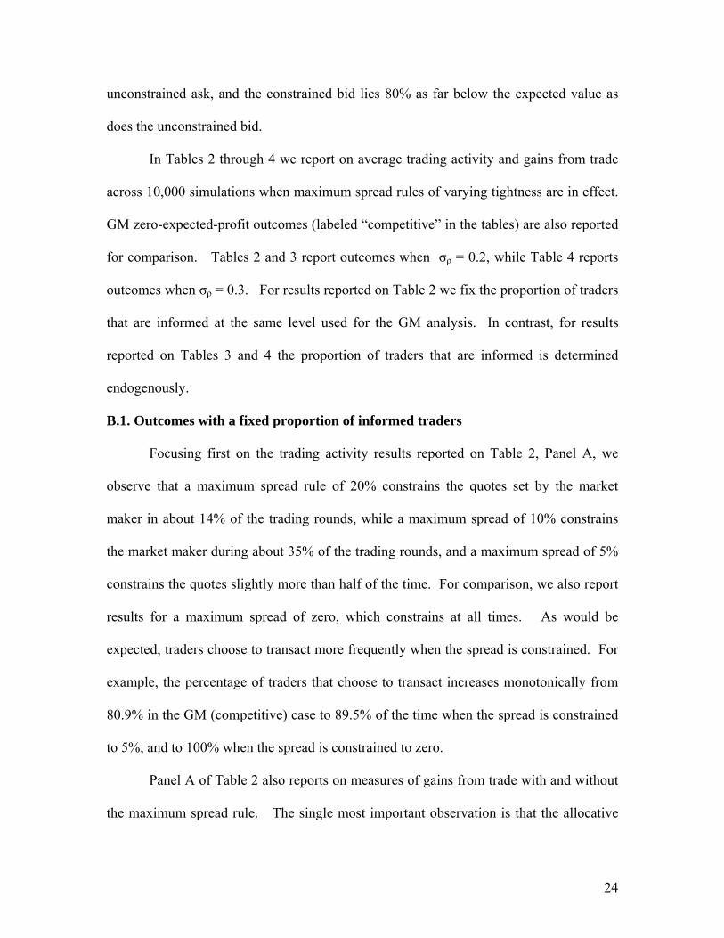
In Tables 2 through 4 we report on average trading activity and gains from trade

across 10,000 simulations when maximum spread rules of varying tightness are in effect.

GM zero-expected-profit outcomes (labeled “competitive” in the tables) are also reported

for comparison. Tables 2 and 3 report outcomes when σρ = 0.2, while Table 4 reports

outcomes when σρ = 0.3. For results reported on Table 2 we fix the proportion of traders

that are informed at the same level used for the GM analysis. In contrast, for results

reported on Tables 3 and 4 the proportion of traders that are informed is determined

endogenously.

B.1. Outcomes with a fixed proportion of informed traders

Focusing first on the trading activity results reported on Table 2, Panel A, we

observe that a maximum spread rule of 20% constrains the quotes set by the market

maker in about 14% of the trading rounds, while a maximum spread of 10% constrains

the market maker during about 35% of the trading rounds, and a maximum spread of 5%

constrains the quotes slightly more than half of the time. For comparison, we also report

results for a maximum spread of zero, which constrains at all times. As would be

expected, traders choose to transact more frequently when the spread is constrained. For

example, the percentage of traders that choose to transact increases monotonically from

80.9% in the GM (competitive) case to 89.5% of the time when the spread is constrained

to 5%, and to 100% when the spread is constrained to zero.

Panel A of Table 2 also reports on measures of gains from trade with and without

the maximum spread rule. The single most important observation is that the allocative

25

gains from trade increase in the presence of the maximum spread rule, and more so when

the spread is more constraining. The total allocative gain from trading increases from

6.90 when spreads are set at the zero profit level to 7.25 when the spread is constrained to

zero. Note, however, that the allocative gains from trade remain less than the maximum

possible level (by 9.0%) even with a zero spread, which reflects that some informed

traders still trade in the “wrong” direction because price does not immediately reflect the

true value of the asset.

Implementing a maximum spread rule in a competitive market imposes losses on

market makers, totaling 0.41 when the spread is constrained to 10%, 0.99 when the

spread is constrained to 5%, and 2.35 when the spread is constrained to zero. This

reflects that the maximum spread rule increases market maker losses to informed traders,

and constrains the market maker’s ability to recoup the losses when trading with

uninformed traders. However, the increased gains from trade captured by both informed

and uninformed traders in the presence of the maximum spread rule exceed the market

maker losses. Clearly the market maker would need to be compensated for losses

incurred if a maximum spread rule is imposed in a competitive market. Direct payments

from listed firms to designated market makers are observed on Euronext Paris and

Stockholm Stock Exchange, as noted by Venkataraman and Waisburd (2006) and Anand,

Tanggaard, and Weaver (2006).

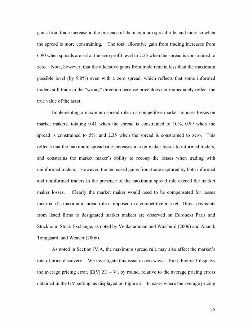
As noted in Section IV.A, the maximum spread rule may also affect the market’s

rate of price discovery. We investigate this issue in two ways. First, Figure 3 displays

the average pricing error, |E(V| Zi) – V|, by round, relative to the average pricing errors

obtained in the GM setting, as displayed on Figure 2. In cases where the average pricing

26

error is larger (smaller) with the maximum spread than in the GM setting Figure 3

displays positive (negative) deviations. Second, in Panel B of Table 2 we report the

percentage of trades that contribute to and detract from price discovery and the difference

between the expected value and the true value of the asset (i.e., the pricing error) after 10

trading rounds and after 40 trading rounds.12

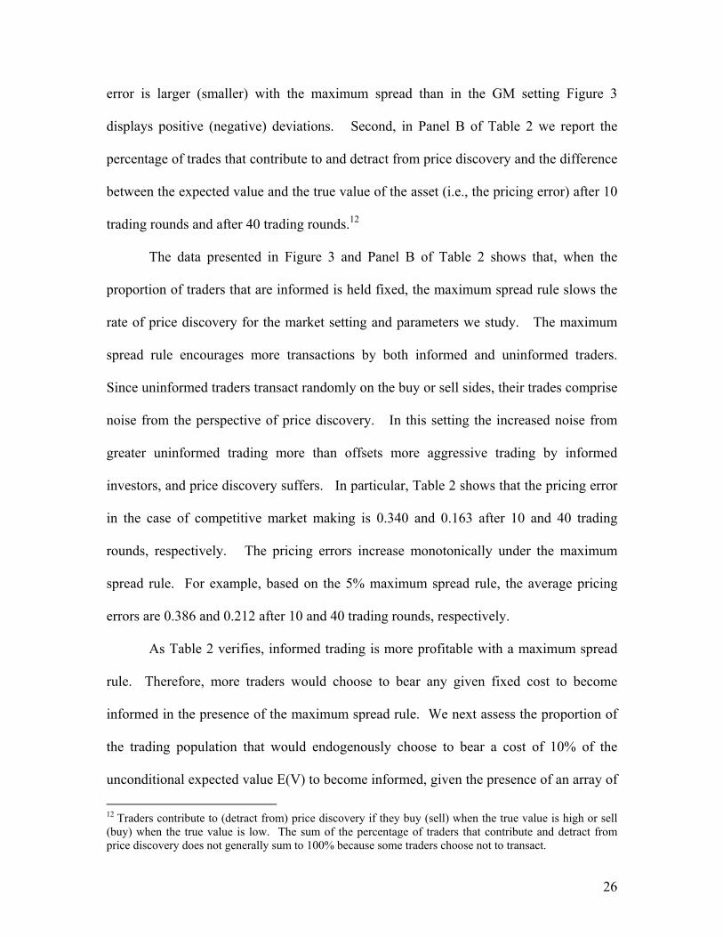
The data presented in Figure 3 and Panel B of Table 2 shows that, when the

proportion of traders that are informed is held fixed, the maximum spread rule slows the

rate of price discovery for the market setting and parameters we study. The maximum

spread rule encourages more transactions by both informed and uninformed traders.

Since uninformed traders transact randomly on the buy or sell sides, their trades comprise

noise from the perspective of price discovery. In this setting the increased noise from

greater uninformed trading more than offsets more aggressive trading by informed

investors, and price discovery suffers. In particular, Table 2 shows that the pricing error

in the case of competitive market making is 0.340 and 0.163 after 10 and 40 trading

rounds, respectively. The pricing errors increase monotonically under the maximum

spread rule. For example, based on the 5% maximum spread rule, the average pricing

errors are 0.386 and 0.212 after 10 and 40 trading rounds, respectively.

As Table 2 verifies, informed trading is more profitable with a maximum spread

rule. Therefore, more traders would choose to bear any given fixed cost to become

informed in the presence of the maximum spread rule. We next assess the proportion of

the trading population that would endogenously choose to bear a cost of 10% of the

unconditional expected value E(V) to become informed, given the presence of an array of

12 Traders contribute to (detract from) price discovery if they buy (sell) when the true value is high or sell (buy) when the true value is low. The sum of the percentage of traders that contribute and detract from price discovery does not generally sum to 100% because some traders choose not to transact.

27

maximum spread rules. The optimal percentage of informed traders is determined

numerically by allowing traders (selected at random) to purchase information. The

equilibrium number of informed traders is determined when the average gain across the

10,000 simulations to the marginal informed trader, relative to the marginal uninformed

trader, is equal to the cost of acquiring information.

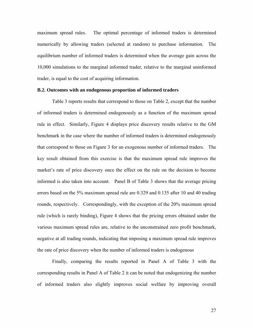
B.2. Outcomes with an endogenous proportion of informed traders

Table 3 reports results that correspond to those on Table 2, except that the number

of informed traders is determined endogenously as a function of the maximum spread

rule in effect. Similarly, Figure 4 displays price discovery results relative to the GM

benchmark in the case where the number of informed traders is determined endogenously

that correspond to those on Figure 3 for an exogenous number of informed traders. The

key result obtained from this exercise is that the maximum spread rule improves the

market’s rate of price discovery once the effect on the rule on the decision to become

informed is also taken into account. Panel B of Table 3 shows that the average pricing

errors based on the 5% maximum spread rule are 0.329 and 0.135 after 10 and 40 trading

rounds, respectively. Correspondingly, with the exception of the 20% maximum spread

rule (which is rarely binding), Figure 4 shows that the pricing errors obtained under the

various maximum spread rules are, relative to the unconstrained zero profit benchmark,

negative at all trading rounds, indicating that imposing a maximum spread rule improves

the rate of price discovery when the number of informed traders is endogenous

Finally, comparing the results reported in Panel A of Table 3 with the

corresponding results in Panel A of Table 2 it can be noted that endogenizing the number

of informed traders also slightly improves social welfare by improving overall

28

allocational efficiency. This reflects the fact that more rapid price discovery reduces

incentives for informed traders to transact in the wrong direction, as noted in Section

IV.A above.

B.3. Sensitivity: Outcomes with greater variation in the desire to trade

Cross-sectional variation in traders’ subjective valuations is required to generate

trade in the GM setting. To ascertain whether the insights obtained here are robust to

variation in the key parameter describing such cross-sectional variation, Table 4 reports

results for the case when σρ = 0.3 that correspond to those reported in Table 3 for the case

when σρ = 0.2 and where the number of informed traders is endogenous. In general,

increasing the cross-sectional variation in the traders’ valuations makes traders less price

sensitive. Comparing Panel A of Table 4 to Panel A of Table 3 it can be noted that when

σρ = 0.3, a 20% maximum spread rule never constrains the quotes. When σρ = 0.2,

however, a 20% maximum spread rule constrains the quotes in 16.6% of the trading

rounds. This result reverses, however, when tighter maximum spread rules are imposed.

For example, under a 5% maximum spread rule, the quotes are constrained in 52.6% of

the trading rounds when σρ = 0.3 compared to 45.5% of the trading rounds when σρ = 0.2.

It can also be noted that increasing the cross-sectional variation in traders’

subjective valuations has two effects on social welfare. First, when σρ = 0.3, social

welfare obtained in the case of competitive market making is closer to the maximum

obtainable. As seen in Table 4, in the competitive case, social welfare is 8.6% lower than

the maximum obtainable. When σρ = 0.2, the competitive case results in social welfare

that is 13.5% below the maximum obtainable. The second is that social welfare is less

sensitive to changes in the maximum spread rule when σρ = 0.3. For example, when the

29

maximum spread rule is 5% and σρ = 0.3, social welfare is 7.7% below the maximum

obtainable, an improvement of 0.9%. When σρ = 0.2, however, the maximum spread rule

of 5% corresponds to an improvement in social welfare of 3.9% relative to the

competitive case.

A similar result holds with respect to price discovery. As shown in Panel B of

Table 4 and in Figure 5, although price discovery is still improved relative to the

competitive case, the effects of the maximum spread rule on the rate of price discovery

are much smaller than in the case where σρ = 0.2. For example, when σρ = 0.3, the

pricing errors are 0.376 and 0.203 after 10 and 40 trading rounds, respectively when

market making is competitive. Under a 5% maximum spread rule, the pricing errors are

0.376 and 0.193 after 10 and 40 trading rounds, respectively.

To summarize, the maximum spread rule has less dramatic effects when cross-

sectional variation in the parameter describing the subjective desire to trade, ρ, is

increased. More variation in ρ implies that uninformed traders are less sensitive to

spreads, and informed traders trade less aggressively on their private information, leading

to narrower competitive spreads. The maximum spread rule has a smaller effect on the

incentives of traders to become informed when there is more cross-sectional variation in

ρ, implying a weaker effect on the rate of price discovery.

C. Outcomes When Market Makers Have Market Power

The results reported in Tables 2 through 4 show that imposing the maximum

spread rule in a competitive marketplace improves allocative efficiency and the speed of

price discovery, but imposes losses on market makers, and hence would require a side

30

payment or subsidy to the market maker charged with posting the quotes that narrow the

spread relative to the GM benchmark.

Though the assumption of zero expected profits is standard in leading

microstructure models, including Glosten and Milgrom (1985) and Kyle (1985), it is

unclear whether competition among liquidity providers is sufficiently intense to yield

zero mean profits in all actual markets. Glosten (1989) models the case of a monopolist

liquidity provider, and in the model presented by Bernhardt and Hughson (1997), market

makers earn positive expected profits in equilibrium.

We next assess the effect of a maximum spread rule when market makers would

otherwise earn positive profits. The specialist on the NYSE trading floor faces

competition from limit orders, but enjoys an information advantage as compared to off-

exchange suppliers of limit orders. 13 We focus for analytical convenience on the

simplified case where the market maker has a monopoly on liquidity provision. We then

examine how constraining the monopolist with affirmative obligations affects outcomes.

We continue to rely on the GM sequential trade framework, but assume that the

monopolist market maker will set quotes that maximize expected profits in each trading

round, unless the resulting spreads are wider than a specified percentage of the

conditional expected asset value, E(V| Zi).14 In general the maximum spread rule in this

setting tends to constrain spreads most often in the early rounds of the simulation, (i.e. in

the wake of the information event), but does not constrain, (and thus allows positive

expected profit spreads) in the later rounds of trading. This allows the market maker to

13 Ready (1999) provides empirical evidence that the NYSE specialist uses her information advantage to trade against market orders that are on average more profitable, while allowing less profitable orders to trade against the limit order book. 14 As closed form solutions for profit-maximizing quotes do not appear to exist in the GM setting, we instead ascertain the quotes that maximize expected profits by a numerical search.

31

earn profits during tranquil periods that can partially or fully (depending on the width of

the maximum allowable spread) offset losses incurred in the wake of the information

event. This setting is generally similar to that modeled by Glosten (1989), except that he

focused on the market maker’s endogenous decision to use profits on small trades to

subsidize losses on large trades at a point in time, while we study the intertemporal

effects as profits earned during tranquil periods are used to offset losses imposed by the

affirmative obligation to narrow spreads that are suffered in the wake of information

events.

Average profit maximizing spreads by trading round are displayed on Figure 1.

Not surprisingly, these are substantially wider than zero-expected profit spreads. Table 5

reports on trading activity and gains from trade with a monopolist market maker, with

and without imposition of maximum spread rules, for the case where σρ = 0.2. 15

Focusing initially on the results for unconstrained profit maximizing spreads, several

results are noteworthy. By comparison to corresponding results for the competitive

benchmark as reported on Table 3, we observe that market maker monopoly pricing leads

to a smaller percentage of traders choosing to become informed, less trading activity, and

reduced gains from trade accruing to informed traders, uninformed traders, and most

importantly, to society as a whole. Further, Figure 2 displays the average pricing error by

trading round with a monopolist market maker. Price discovery is slowed by the wide

monopolist spreads, as less traders choose to become informed. Unconstrained

monopoly pricing by the liquidity provider degrades market quality in each dimension

that we consider.

15 Results reported are based on σρ = 0.2. Conclusions obtained when while setting σρ = 0.3 are similar. Results also allow the number of informed traders to be determined endogenously.

32

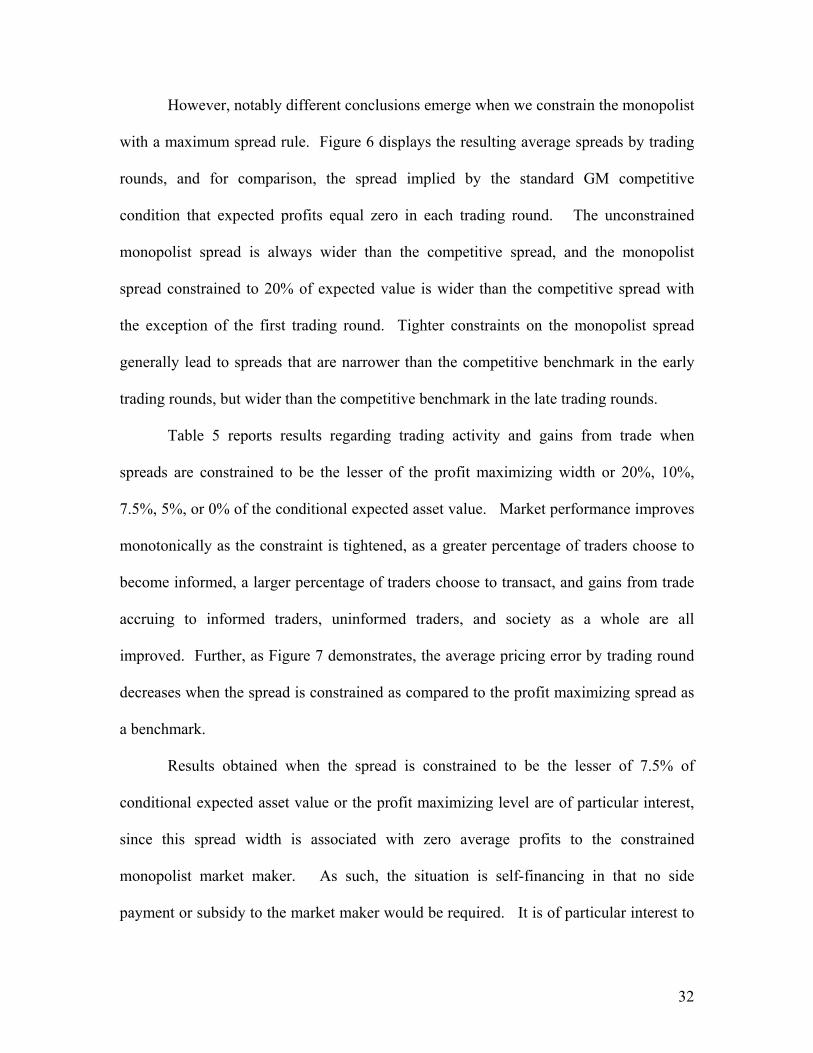
However, notably different conclusions emerge when we constrain the monopolist

with a maximum spread rule. Figure 6 displays the resulting average spreads by trading

rounds, and for comparison, the spread implied by the standard GM competitive

condition that expected profits equal zero in each trading round. The unconstrained

monopolist spread is always wider than the competitive spread, and the monopolist

spread constrained to 20% of expected value is wider than the competitive spread with

the exception of the first trading round. Tighter constraints on the monopolist spread

generally lead to spreads that are narrower than the competitive benchmark in the early

trading rounds, but wider than the competitive benchmark in the late trading rounds.

Table 5 reports results regarding trading activity and gains from trade when

spreads are constrained to be the lesser of the profit maximizing width or 20%, 10%,

7.5%, 5%, or 0% of the conditional expected asset value. Market performance improves

monotonically as the constraint is tightened, as a greater percentage of traders choose to

become informed, a larger percentage of traders choose to transact, and gains from trade

accruing to informed traders, uninformed traders, and society as a whole are all

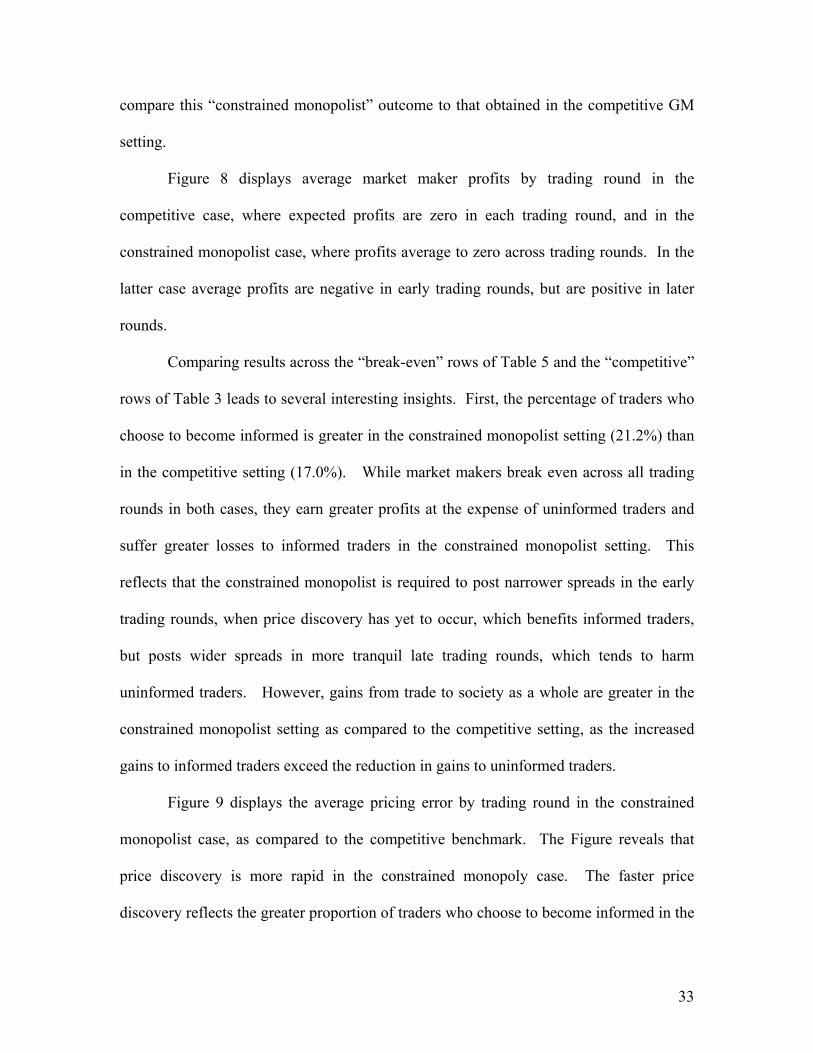
improved. Further, as Figure 7 demonstrates, the average pricing error by trading round

decreases when the spread is constrained as compared to the profit maximizing spread as

a benchmark.

Results obtained when the spread is constrained to be the lesser of 7.5% of

conditional expected asset value or the profit maximizing level are of particular interest,

since this spread width is associated with zero average profits to the constrained

monopolist market maker. As such, the situation is self-financing in that no side

payment or subsidy to the market maker would be required. It is of particular interest to

33

compare this “constrained monopolist” outcome to that obtained in the competitive GM

setting.

Figure 8 displays average market maker profits by trading round in the

competitive case, where expected profits are zero in each trading round, and in the

constrained monopolist case, where profits average to zero across trading rounds. In the

latter case average profits are negative in early trading rounds, but are positive in later

rounds.

Comparing results across the “break-even” rows of Table 5 and the “competitive”

rows of Table 3 leads to several interesting insights. First, the percentage of traders who

choose to become informed is greater in the constrained monopolist setting (21.2%) than

in the competitive setting (17.0%). While market makers break even across all trading

rounds in both cases, they earn greater profits at the expense of uninformed traders and

suffer greater losses to informed traders in the constrained monopolist setting. This

reflects that the constrained monopolist is required to post narrower spreads in the early

trading rounds, when price discovery has yet to occur, which benefits informed traders,

but posts wider spreads in more tranquil late trading rounds, which tends to harm

uninformed traders. However, gains from trade to society as a whole are greater in the

constrained monopolist setting as compared to the competitive setting, as the increased

gains to informed traders exceed the reduction in gains to uninformed traders.

Figure 9 displays the average pricing error by trading round in the constrained

monopolist case, as compared to the competitive benchmark. The Figure reveals that

price discovery is more rapid in the constrained monopoly case. The faster price

discovery reflects the greater proportion of traders who choose to become informed in the

34

constrained monopolist case, which in turn reflects that spreads are constrained during

the early rounds of trading when profit opportunities to informed traders are greatest.

To conclude, this analysis demonstrates that market performance can be improved

by imposing a maximum spread rule on a monopolist market maker, and that the

performance improvement is greater when the constraint is more binding. Outcomes

observed when the constraint reduces monopolist profits to zero on average are of

particular interest, since in contrast to the case when a binding spread rule is imposed in a

competitive setting, the market maker would not require a subsidy or side payment. We

find that constraining the spread such that the monopolist market maker earns zero

average profits produces superior overall outcomes in terms of allocative efficiency and

more rapid price discovery as compared to the competitive setting. However,

distributional issues arise, as uninformed traders gain less from trading with the

constrained monopolist as compared to the competitive setting.

D. Outcomes Under a Price-Continuity Rule

Although a maximum spread rule is the most frequently encountered form of

affirmative obligation, the world’s largest stock market, the NYSE, instead uses a “price-

continuity rule” by which price movements between successive transactions are limited

to be less than some pre-specified value. However, as noted, the NYSE price-continuity

rule is rooted in government regulation, while markets appear to have adopted maximum

spread rules endogenously. In this section we briefly describe some insights obtained

when the Glosten-Milgrom sequential trade model is simulated subject to a constraint

limiting the bid and ask prices at time t such that:

Pt-1- k < Bt

35

and

At < Pt-1+k,

where Pt-1 is the previous transaction price and k is a constant specified as a percentage of

the conditional expected value of the asset. That is, the bid price cannot be less, nor can

the ask price exceed, the prior trade price by more than a specified amount, k. As

compared to the maximum spread rule, this implementation of the price continuity rule

has the additional effect of constraining the location of the bid and ask quotes relative to

conditional expected value, and in general will limit the movement of the quotes in

response to information contained in the prior trade.

The results obtained from simulating the Glosten-Milgrom model subject to the

price continuity rule are presented in Table 6, for the case where σρ = 0.2 and where the

number of informed traders is determined endogenously. The most striking result in the

table is that the gains in allocative efficiency are not monotonic across different declining

values of the price continuity parameter (k). Specifically, as seen in the last column of

Panel A in the table, allocative efficiency is maximized when the price continuity

parameter is equal to 10%. The allocative efficiency is similar to the corresponding value

under a 10% maximum spread rule presented in Table 3. A similar nonmonotonic pattern

appears in the fraction of traders that choose to become informed, although the maximum

fraction of informed traders appears at a value of 5% for the price continuity constraint.

Panel B reports the results for price discovery. When price discovery is measured

based on the difference between the transaction price and the true value, as in columns 4

and 5, the results indicate that price discovery is generally slower compared to the speed

of price discovery under a similar maximum spread rule as reported in Table 3. This

36

result is intuitive because the price continuity rule keeps prices from moving more than a

prespecified amount after each trade. However, this measure of price discovery is

potentially misleading, because rational traders engaged in Bayesian updating understand

the implications of the rule and adjust their conditional expectations of asset value

accordingly. When price discovery is measured as the difference between the conditional

expectation of asset value and the true value as in columns 6 and 7, a different picture

emerges. In this case, price discovery by trading round forty is improved with tighter

price continuity constraints, the overall speed of price discovery is similar to that

obtained under a maximum spread rule, and in some cases (i.e., when the price continuity

constraint is set very tightly) exceeds that for the corresponding maximum spread rule.

This somewhat counterintuitive result arises from the fact that when the price is

artificially held away from its true value by a price continuity rule, then more traders,

including those not privately informed, detect the mispricing and trade in the direction

(buying undervalued assets and selling overvalued assets) that speeds price discovery.

For example, Table 6 shows that a price continuity rule set at 1% leads to 77.9% of

traders speeding price discovery, while by comparison Table 2 shows that a maximum

spread rule of 1% led (with otherwise identical parameters) to 54.7% of traders speeding

price discovery. This leads to more rapid updating of the conditional expected value

under the price continuity rule, despite slower adjustment in transaction prices. Note,

however, that an empirical researcher relying on transaction prices only would not detect

the more rapid updating of conditional expected values, and would underestimate the

speed of price discovery in the presence of a price continuity rule.

37

Overall, the effects of a price continuity rule are more complex than the effects of

the maximum spread rule, and the simulation serves to point out some of the intricacies

associated with differing types of affirmative obligations that might be imposed on the

market maker.

V. Conclusions

In this paper, we consider why most financial markets, including electronic stock

exchanges, choose to designate one or more agents as market makers, who agree to take

on certain affirmative obligations to provide liquidity. We note that the answer to the

question we pose cannot simply be “because liquidity is valuable”, because profit seeking

behavior should induce the provision of the socially optimal amount of liquidity, under

standard competitive market assumptions.

We demonstrate two reasons it can be socially efficient to specify affirmative

obligations for designated market makers, focusing in particular on the obligation to

maintain a quoted bid-ask spread that does not exceed a specified level, while relying on

the sequential trade framework of Glosten and Milgrom (1985) As they emphasize, the

bid-ask spread is, in part, an informational phenomenon, allowing the market maker to

recoup from uninformed traders the losses incurred in transacting with better-informed

traders. However, the informational component of the spread is a transfer rather than a

cost from the viewpoint of society as a whole. Some traders, for whom the potential

gain from trade is less than the spread, are dissuaded from trading by the spread. One

reason that a maximum spread rule improves social welfare is that more investors will

choose to trade when the spread is narrower, resulting in improved allocative efficiency

38

Increased trading enhances efficiency as long as the spread is not constrained to be less

than the social cost of completing trades.

The second social benefit attributable to a maximum spread rule can arise due to

improved price discovery. A maximum spread rule improves the profitability of being

informed and incentives to become informed. When we allow the percentage of the

trading population that is informed to vary endogenously as a function of the spread rule

in effect we find that the rate of price discovery is improved by the existence a maximum

spread rule. Whether social efficiency is also enhanced by the increase in informed

trading resulting from a maximum spread rule depends on a balance of cost and benefits.

If more traders choose to incur costs of becoming informed, then total information

gathering costs are increased. However, more rapid price discovery provides superior

information for real decisions, leading to improved economic efficiency. Modeling the

efficiency gains arising from superior real decisions occasioned by more accurate

financial market prices is beyond the scope of this paper.

As might be expected, we document improved allocative efficiency and faster

price discovery when a maximum spread rule is used to narrow spreads as compared to

those that maximize expected profits for a monopolist market maker. More surprisingly,

we document that constraining spreads so that the monopolist market maker earns zero

average profits across trading rounds leads to improved allocative efficiency and price

discovery as compared to the competitive outcome, which requires zero expected profits

in each trading round. This result indicates that a allowing designated market makers to

have some monopoly power or information advantage while constraining profits with a

maximum spread rule can be an efficient market design.

39

Our analysis implies that affirmative obligations such as a maximum spread rule

will be efficient when market markers possess a non-trivial degree of market power, or,

since it is the asymmetric information component of the competitive spread that leads to

inefficient reductions in trading, when asymmetric information costs are large. Thus, our

analysis differs in an important but subtle way from the conventional wisdom that

designated market makers are required in otherwise illiquid stocks. If a stock is illiquid

due to large real frictions, i.e. high order-processing or inventory costs, e.g. due to a lack

of a broad investor base or because investors are following buy-and-hold strategies, then

the marginal social cost of providing liquidity is high, and it is socially efficient for

spreads to be wide. That is, our analysis provides no role for affirmative obligations for

thinly traded securities in the absence of substantive information asymmetries. In

contrast, if the wide spreads reflect a high degree of information asymmetry, then

efficiency can be enhanced by a constraining spreads to be narrower.

In contrast to the NYSE’s price continuity rule, which as Stoll (1998) notes is

rooted in government regulation, maximum spread rules appear to have been adopted

voluntarily by a number of financial markets. A maximum spread rule can be viewed as

a market response to a market imperfection arising from informational externalities. We

view this paper as a useful start towards a comprehensive theory of endogenous, market-

determined affirmative obligations. However, several limitations and possible extensions

can be noted. We focus primarily only on only one type of market maker obligation, the

commitment to maintain narrow spreads. We have not attempted to assess the optimal

set of affirmative obligations or how these might vary across stocks or markets. Further,

since the GM framework focuses on traders who arrive sequentially in an exogenously

40

determined order, and who transact either zero or one unit, we have not considered

potential effects on trade timing, trade sizes, repeat trading, or trading aggressiveness. .

Further, though we document that affirmative obligations can affect the rate of price

discovery, our analysis measures only the efficiency with which existing shares are

allocated across traders; we do not capture efficiency gains which would result from

changes in real decisions attributable to better price discovery. Finally, we have not

provided a formal analysis of the important question of how market makers should

optimally be compensated for taking on affirmative obligations to supply liquidity. Each

of these limitations highlights useful opportunities for future research.

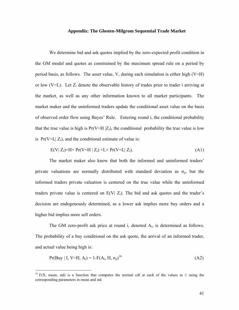
41

Appendix: The Glosten-Milgrom Sequential Trade Market

We determine bid and ask quotes implied by the zero-expected profit condition in

the GM model and quotes as constrained by the maximum spread rule on a period by

period basis, as follows. The asset value, V, during each simulation is either high (V=H)

or low (V=L). Let Zi denote the observable history of trades prior to trader i arriving at

the market, as well as any other information known to all market participants. The

market maker and the uninformed traders update the conditional asset value on the basis

of observed order flow using Bayes’ Rule. Entering round i, the conditional probability

that the true value is high is Pr(V=H |Zi), the conditional probability the true value is low

is Pr(V=L| Zi), and the conditional estimate of value is:

E(V| Zi)=H× Pr(V=H | Zi) +L× Pr(V=L| Zi). (A1)

The market maker also know that both the informed and uninformed traders’

private valuations are normally distributed with standard deviation as σρ, but the

informed traders private valuation is centered on the true value while the uninformed

traders private value is centered on E(V| Zi). The bid and ask quotes and the trader’s

decision are endogenously determined, as a lower ask implies more buy orders and a

higher bid implies more sell orders.

The GM zero-profit ask price at round i, denoted Ai, is determined as follows.

The probability of a buy conditional on the ask quote, the arrival of an informed trader,

and actual value being high is:

Pr(Buy | I, V=H, Ai) = 1-F(Ai, H, σρ)16 (A2)

16 F(X, mean, std) is a function that computes the normal cdf at each of the values in X using the corresponding parameters in mean and std.

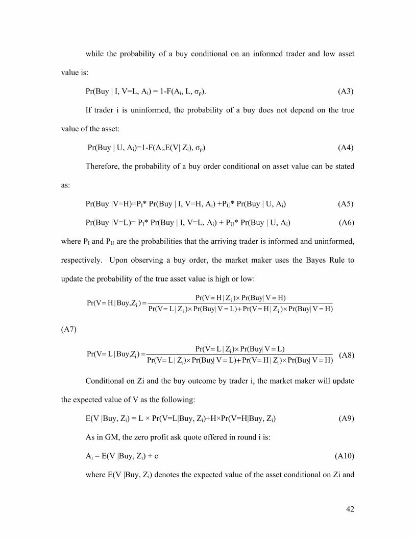
42

while the probability of a buy conditional on an informed trader and low asset

value is:

Pr(Buy | I, V=L, Ai) = 1-F(Ai, L, σρ). (A3)

If trader i is uninformed, the probability of a buy does not depend on the true

value of the asset:

Pr(Buy | U, Ai)=1-F(Ai,E(V| Zi), σρ) (A4)

Therefore, the probability of a buy order conditional on asset value can be stated

as:

Pr(Buy |V=H)=PI* Pr(Buy | I, V=H, Ai) +PU* Pr(Buy | U, Ai) (A5)

Pr(Buy |V=L)= PI* Pr(Buy | I, V=L, Ai) + PU* Pr(Buy | U, Ai) (A6)

where PI and PU are the probabilities that the arriving trader is informed and uninformed,

respectively. Upon observing a buy order, the market maker uses the Bayes Rule to

update the probability of the true asset value is high or low:

H)V|Pr(Buy )Z|HPr(VL)V|Pr(Buy )Z|LPr(V

H)V|Pr(Buy )Z|HPr(V ) ZBuy, |HPr(V

ii

ii =×=+=×=

=×===

(A7)

H)V|Pr(Buy )Z|HPr(VL)V|Pr(Buy )Z|LPr(V

L)V|Pr(Buy )Z|LPr(V ) ZBuy, |LPr(Vii

ii =×=+=×=

=×=== (A8)

Conditional on Zi and the buy outcome by trader i, the market maker will update

the expected value of V as the following:

E(V |Buy, Zi) = L × Pr(V=L|Buy, Zi)+H×Pr(V=H|Buy, Zi) (A9)

As in GM, the zero profit ask quote offered in round i is:

Ai = E(V |Buy, Zi) + c (A10)

where E(V |Buy, Zi) denotes the expected value of the asset conditional on Zi and

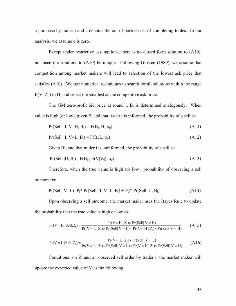
43

a purchase by trader i and c denotes the out of pocket cost of completing trades. In our

analysis, we assume c is zero.

Except under restrictive assumptions, there is no closed form solution to (A10),

nor need the solutions to (A10) be unique. Following Glosten (1989), we assume that

competition among market makers will lead to selection of the lowest ask price that

satisfies (A10). We use numerical techniques to search for all solutions within the range

E(V| Zi ) to H, and select the smallest as the competitive ask price.

The GM zero-profit bid price at round i, Bi is determined analogously. When

value is high (or low), given Bi and that trader i is informed, the probability of a sell is:

Pr(Sell | I, V=H, Bi) = F(Bi, H, σρ) (A11)

Pr(Sell | I, V=L, Bi) = F(Bi,L, σρ) (A12)

Given Bi, and that trader i is uninformed, the probability of a sell is:

Pr(Sell |U, Bi) =F(Bi , E(V| Zi), σρ) (A13)

Therefore, when the true value is high (or low), probability of observing a sell

outcome is:

Pr(Sell |V=L)=PI* Pr(Sell | I, V=L, Bi) + PU* Pr(Sell |U, Bi) (A14)

Upon observing a sell outcome, the market maker uses the Bayes Rule to update

the probability that the true value is high or low as:

H)V|Pr(Sell )Z|HPr(VL)V|Pr(Sell )Z|LPr(V

H)V|Pr(Sell )Z|HPr(V ) ZSell, |HPr(Vii

ii =×=+=×=

=×=== (A15)

H)V|Pr(Sell )Z|HPr(VL)V|Pr(Sell )Z|LPr(V

L)V|Pr(Sell )Z|LPr(V ) ZSell, |LPr(Vii

ii =×=+=×=

=×=== (A16)

Conditional on Zi and an observed sell order by trader i, the market maker will

update the expected value of V as the following:

44

E(V|Sell, Zi)= L × Pr(V=L|Sell, Zi) + H×Pr(V=H|Sell, Zi) (A17)

The GM bid quote offered to trader i is

Bi = E(V |Sell, Zi) + c (A18)

where E(V |Sell, Zi) denotes the expected value of the asset conditional on Zi and a sell

by trader i and c denotes the social cost of completing trades. We also select the actual

bid quote by a numerical search over the range L to E(V|Zi), and select the maximum bid

among the solutions to (A18) as the GM quote.

Observing the bid and ask quotes (Bi and Ai), trader i buys if her own value (for

an informed trader V+ ρi, for uniformed trader E(V|Zi)+ ρi exceeds the ask, and sells if

her value is below the bid. If her subjective valuation is between the bid and the ask she

does not trade. Based on the outcome (buy, sell, or no trade), the market maker

recalculates conditional probabilities. The new conditional probability is the market

makers posterior probability of the event, and hence it incorporates the new information

he has learned from observing the trade.

If there is a buy at round i,

Pr(V=H | Zi+1) = Pr(V=H | Buy, Zi) (A19)

Pr(V=L | Zi+1) = Pr(V=L | Buy, Zi) (A20)

If there is a sell at round i,

Pr(V=H | Zi+1) = Pr(V=H | Sell, Zi) (A21)

Pr(V=L | Zi+1) = Pr(V=L | Sell, Zi) (A22)

If there is no trade at round i,

Pr(V=H | Zi+1) = Pr(V=H | No Trade, Zi) (A23)

Pr(V=L | Zi+1) = Pr(V=L | No Trade, Zi) (A24)

45

Where Pr(V=H | No Trade, Zi)= 1- Pr(V=H | Buy, Zi)- Pr(V=H | Sell, Zi) (A25)

And Pr(V=L | No Trade, Zi)= 1- Pr(V=L | Buy, Zi)- Pr(V=L | Sell, Zi) (A26)

The posterior conditional probability from round i then becomes the market

makers new prior to set the expected value E(V|Zi+1) competitive bid Bi+1 and ask price

Ai+1. Trader i+1 arrives, makes her decision, and the market maker updates using Bayes’

rule, and the process continues.

We incorporate a maximum spread rule as follows. All parameters, including

trader’s subjective valuations, are the same as in the GM setting. Letting the superscript

C denote a constrained quote and the superscript U denote an unconstrained (zero

expected profit) quote, we select constrained ask and bid quotes at the arrival of trader i

such that:

Uii

Cii

iUi

iCi

Ui

Ui

Ci

Ci

BZVEBZVE

ZVEAZVEA

BABA

−

−=

−

−=

−

−

)|()|(

)|()|( (A27)

When the constraint is not binding the bid and ask quotes are set as in GM so that

expected profit conditional on a trade is zero.17 When the constraint is binding, the ask

and bid quotes are adjusted toward each other in order to meet the constraint.

17 However, the quotes in this case generally differ from those that would have prevailed in the same round in the absence of a maximum spread rule, because constraints on quotations in earlier trading rounds will generally have altered earlier trading decisions, which affects the conditional expected asset value.

46

References

Anand, A., and D. G. Weaver, 2006, “The Value of the specialist: Empirical evidence from the CBOE”, Journal of Financial Markets, forthcoming. Anand, A., C. Tanggaard, and D. G. Weaver, 2006, “Paying for Market Quality”, working paper, Rutgers University. Battalio, R., and C. Holden, 2001, “A Simple Model of Payment for Order Flow, Internalization, and Total Trading Cost,” Journal of Financial Markets, 4, 33-71. Bernhardt, D. and E. Hughson, 1997, “Splitting Orders”, Review of Financial Studies, 10, 69-101. Charitou and Panayides, 2006, “The Role of the Market Maker in International Capital Markets: Challenges and Benefits of Implementation in Emerging Markets”, working paper, University of Utah. Demsetz, H. 1968 “The Cost of Transacting”, Quarterly Journal of Economics, 82, 33-53. Dutta, P.K., A. Madhavan, 1997, “Competition and collusion in dealer markets”, Journal of Finance, 52(1) 245-276. Glosten, L. and P. Milgrom, 1985, “Bid, Ask, and Transaction Prices in a Specialist Market with Heterogeneously Informed Traders”, Journal of Financial Economics, 14, 71-100. Glosten, L., 1989, “Insider Trading, Liquidity and the Role of the Monopoly Specialist,” Journal of Business, 62, 211-235. Harris, L. and V. Panchapagesan, 2005, The information content of the limit order book: Evidence from NYSE specialist trading decisions, Journal of Financial Markets, 8, 25-67. Hasbrouck, J., Sofianos, G., 1993. The Trades of Market Makers: An Empirical Analysis of NYSE Specialists. Journal of Finance 48(5), 1975–1199. Hollifield, B., Miller, R., Sandas, P. and Slive , J. “Liquidity Supply and Demand in Limit Order Markets.” Journal of Finance, forthcoming Holmstrom, B., and J. Tirole, 1993, “Market Liquidity and Performance Monitoring”, Journal of Political Economy, 101, 678-709. Ho, T., and H. Stoll, 1980 “On Dealer Markets Under Competition” The Journal of Finance, Vol. 35, 259-267.

47

Jacklin, C., A. Kleidon, and P. Pfeiderer, 1992, “Underestimation of Portfolio Insurance and the Crash of October 1987”, Review of Financial Studies, 5, 35-63. Kandel and Marx, 1997, Nasdaq market structure and spread patterns, Journal of Financial Economics 45, No. 1, 61-90. Kyle, A., 1985, “Continuous Auctions and Insider Trading”, Econometrica, 53, 1315-1336. Madhavan, A., Smidt, S., 1993, An analysis of daily changes in specialist inventories and quotations, Journal of Finance 48, 1595-1628. Panayides, M., 2006, “Affirmative Obligations and Market Making with Inventory,” working paper, Journal of Financial Economics, forthcoming. Petrella, G., and M. Nimalendran, 2003, “Do Thinly-Traded Stocks Benefit from Specialist Intervention”? Journal of Banking and Finance, 27, 1823-1854. Ready, Mark J., 1999, “The Specialist’s Discretion: Stopped Orders and Price Improvement”, Review of Financial Studies, 12, 1075-1112 Rock, K., 1996, “The Specialist’s Order Book and Price Anomalies” Review of Financial Studies, forthcoming Sabourin, D. 2006, “Are Designated Market Makers Necessary in Centralized Limit Order Markets?”, working paper, Université Paris IX Dauphine. Seppi, Duane J., 1997, “Liquidity Provision with Limit Orders and Strategic Specialist”, Review of Financial Studies, 10, 103-150. Stoll, H. 2000, “Friction”, Journal of Finance, 55, 1470-1514. Stoll, H., 1998, “Reconsidering the Affirmative Obligations of Market Makers”, Financial Analysts Journal, September/October, 72-82. Subrahmanyam, A., and S. Titman, 1999, “The Going-Public Decision and the Development of Financial Markets”, Journal of Finance, 54, 1045-1082. Tetlock, P., and R. Hahn, 2007, “Optimal Liquidity Provision for Decision Makers” working paper, University of Texas at Austin. Venkataraman, K., Waisburd, A., 2006, The Value of the Designated Market Maker, Journal of Financial and Quantitative Analysis, forthcoming.

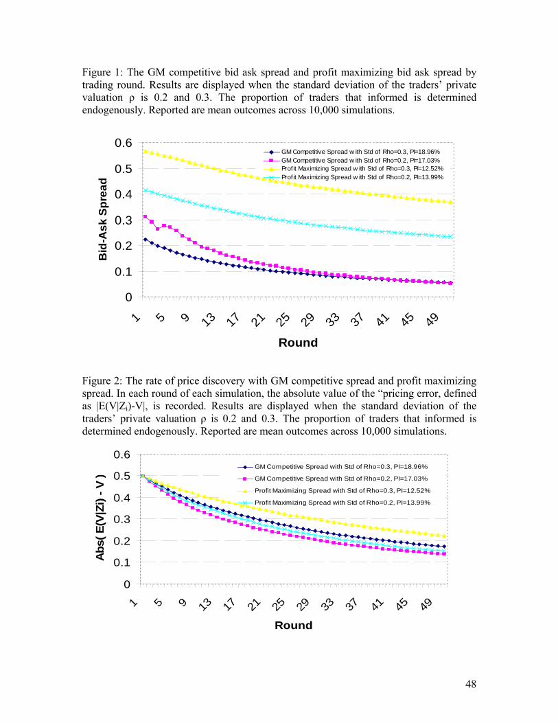
48

Figure 1: The GM competitive bid ask spread and profit maximizing bid ask spread by trading round. Results are displayed when the standard deviation of the traders’ private valuation ρ is 0.2 and 0.3. The proportion of traders that informed is determined endogenously. Reported are mean outcomes across 10,000 simulations.

0

0.1

0.2

0.3

0.4

0.5

0.6

1 5 9 13 17 21 25 29 33 37 41 45 49

Round

Bid

-Ask

Spr

ead

GM Competitive Spread w ith Std of Rho=0.3, PI=18.96%GM Competitive Spread w ith Std of Rho=0.2, PI=17.03%Profit Maximizing Spread w ith Std of Rho=0.3, PI=12.52%Profit Maximizing Spread w ith Std of Rho=0.2, PI=13.99%

Figure 2: The rate of price discovery with GM competitive spread and profit maximizing spread. In each round of each simulation, the absolute value of the “pricing error, defined as |E(V|Zi)-V|, is recorded. Results are displayed when the standard deviation of the traders’ private valuation ρ is 0.2 and 0.3. The proportion of traders that informed is determined endogenously. Reported are mean outcomes across 10,000 simulations.

0

0.1

0.2

0.3

0.4

0.5

0.6

1 5 9 13 17 21 25 29 33 37 41 45 49

Round

Abs

( E(V

|Zi)

- V )

GM Competitive Spread with Std of Rho=0.3, PI=18.96%

GM Competitive Spread with Std of Rho=0.2, PI=17.03%

Profit Maximizing Spread with Std of Rho=0.3, PI=12.52%

Profit Maximizing Spread with Std of Rho=0.2, PI=13.99%

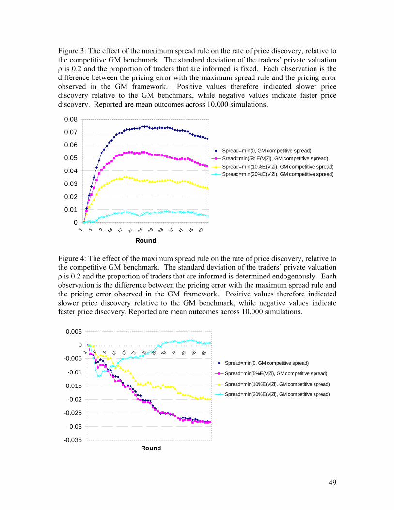
49

Figure 3: The effect of the maximum spread rule on the rate of price discovery, relative to the competitive GM benchmark. The standard deviation of the traders’ private valuation ρ is 0.2 and the proportion of traders that are informed is fixed. Each observation is the difference between the pricing error with the maximum spread rule and the pricing error observed in the GM framework. Positive values therefore indicated slower price discovery relative to the GM benchmark, while negative values indicate faster price discovery. Reported are mean outcomes across 10,000 simulations.

0

0.01

0.02

0.03

0.04

0.05

0.06

0.07

0.08

1 5 9 13 17 21 25 29 33 37 41 45 49

Round

Spread=min(0, GM competitive spread)Sread=min(5%E(V|Zi), GM competitive spread)Spread=min(10%E(V|Zi), GM competitive spread)Spread=min(20%E(V|Zi), GM competitive spread)

Figure 4: The effect of the maximum spread rule on the rate of price discovery, relative to the competitive GM benchmark. The standard deviation of the traders’ private valuation ρ is 0.2 and the proportion of traders that are informed is determined endogenously. Each observation is the difference between the pricing error with the maximum spread rule and the pricing error observed in the GM framework. Positive values therefore indicated slower price discovery relative to the GM benchmark, while negative values indicate faster price discovery. Reported are mean outcomes across 10,000 simulations.

-0.035

-0.03

-0.025

-0.02

-0.015

-0.01

-0.005

0

0.005

1 5 9 13 17 21 25 29 33 37 41 45 49

Round

Spread=min(0, GM competitive spread)

Spread=min(5%E(V|Zi), GM competitive spread)

Spread=min(10%E(V|Zi), GM competitive spread)

Spread=min(20%E(V|Zi), GM competitive spread)

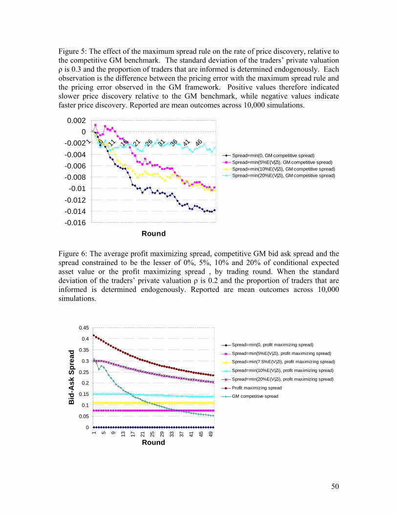
50

Figure 5: The effect of the maximum spread rule on the rate of price discovery, relative to the competitive GM benchmark. The standard deviation of the traders’ private valuation ρ is 0.3 and the proportion of traders that are informed is determined endogenously. Each observation is the difference between the pricing error with the maximum spread rule and the pricing error observed in the GM framework. Positive values therefore indicated slower price discovery relative to the GM benchmark, while negative values indicate faster price discovery. Reported are mean outcomes across 10,000 simulations.

-0.016-0.014-0.012

-0.01-0.008-0.006-0.004-0.002

00.002

1 6 11 16 21 26 31 36 41 46

Round

Spread=min(0, GM competitive spread)Spread=min(5%E(V|Zi), GM competitive spread)Spread=min(10%E(V|Zi), GM competitive spread)Spread=min(20%E(V|Zi), GM competitive spread)

Figure 6: The average profit maximizing spread, competitive GM bid ask spread and the spread constrained to be the lesser of 0%, 5%, 10% and 20% of conditional expected asset value or the profit maximizing spread , by trading round. When the standard deviation of the traders’ private valuation ρ is 0.2 and the proportion of traders that are informed is determined endogenously. Reported are mean outcomes across 10,000 simulations.

0

0.05

0.1

0.15

0.2

0.25

0.3

0.35

0.4

0.45

1 5 9 13 17 21 25 29 33 37 41 45 49

Round

Bid

-Ask

Spr

ead

Spread=min(0, profit maximizing spread)

Spread=min(5%E(V|Zi), profit maximizing spread)

Spread=min(7.5%E(V|Zi), profit maximizing spread)

Spread=min(10%E(V|Zi), profit maximizing spread)

Spread=min(20%E(V|Zi), profit maximizing spread)

Profit maximizing spread

GM competitive spread

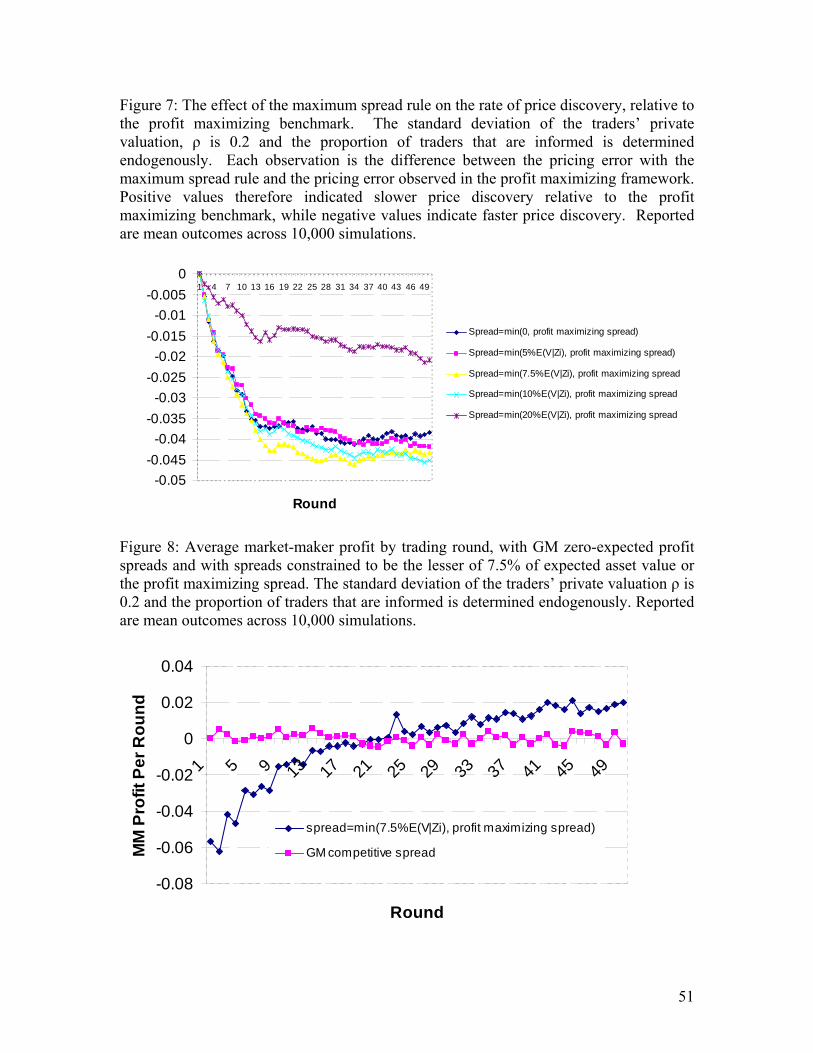
51

Figure 7: The effect of the maximum spread rule on the rate of price discovery, relative to the profit maximizing benchmark. The standard deviation of the traders’ private valuation, ρ is 0.2 and the proportion of traders that are informed is determined endogenously. Each observation is the difference between the pricing error with the maximum spread rule and the pricing error observed in the profit maximizing framework. Positive values therefore indicated slower price discovery relative to the profit maximizing benchmark, while negative values indicate faster price discovery. Reported are mean outcomes across 10,000 simulations.

-0.05-0.045

-0.04-0.035

-0.03-0.025

-0.02-0.015

-0.01-0.005

01 4 7 10 13 16 19 22 25 28 31 34 37 40 43 46 49

Round

Spread=min(0, profit maximizing spread)

Spread=min(5%E(V|Zi), profit maximizing spread)

Spread=min(7.5%E(V|Zi), profit maximizing spread

Spread=min(10%E(V|Zi), profit maximizing spread

Spread=min(20%E(V|Zi), profit maximizing spread

Figure 8: Average market-maker profit by trading round, with GM zero-expected profit spreads and with spreads constrained to be the lesser of 7.5% of expected asset value or the profit maximizing spread. The standard deviation of the traders’ private valuation ρ is 0.2 and the proportion of traders that are informed is determined endogenously. Reported are mean outcomes across 10,000 simulations.

-0.08

-0.06

-0.04

-0.02

0

0.02

0.04

1 5 9 13 17 21 25 29 33 37 41 45 49

Round

MM

Pro

fit P

er R

ound

spread=min(7.5%E(V|Zi), profit maximizing spread)

GM competitive spread

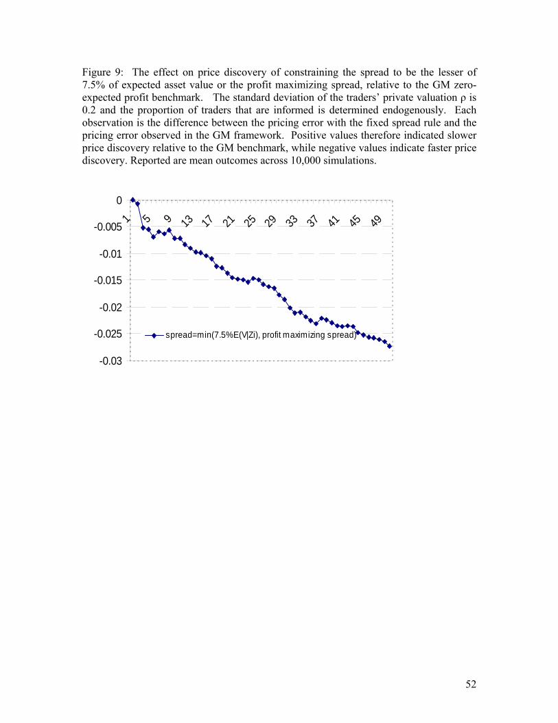
52

Figure 9: The effect on price discovery of constraining the spread to be the lesser of 7.5% of expected asset value or the profit maximizing spread, relative to the GM zero-expected profit benchmark. The standard deviation of the traders’ private valuation ρ is 0.2 and the proportion of traders that are informed is determined endogenously. Each observation is the difference between the pricing error with the fixed spread rule and the pricing error observed in the GM framework. Positive values therefore indicated slower price discovery relative to the GM benchmark, while negative values indicate faster price discovery. Reported are mean outcomes across 10,000 simulations.

-0.03

-0.025

-0.02

-0.015

-0.01

-0.005

0

1 5 9 13 17 21 25 29 33 37 41 45 49

spread=min(7.5%E(V|Zi), profit maximizing spread)

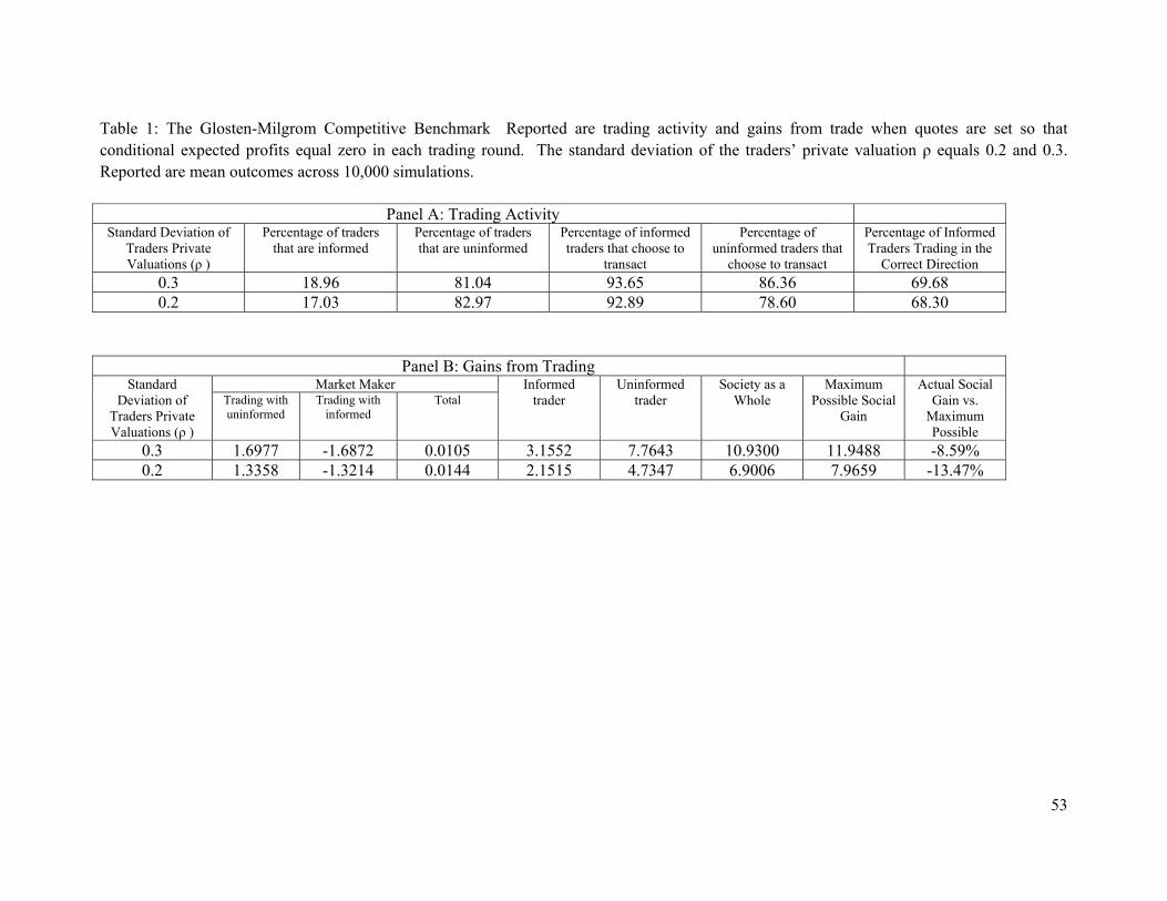
53

Table 1: The Glosten-Milgrom Competitive Benchmark Reported are trading activity and gains from trade when quotes are set so that conditional expected profits equal zero in each trading round. The standard deviation of the traders’ private valuation ρ equals 0.2 and 0.3. Reported are mean outcomes across 10,000 simulations.

Panel A: Trading Activity Standard Deviation of

Traders Private Valuations (ρ )

Percentage of traders that are informed

Percentage of traders that are uninformed

Percentage of informed traders that choose to

transact

Percentage of uninformed traders that

choose to transact

Percentage of Informed Traders Trading in the

Correct Direction 0.3 18.96 81.04 93.65 86.36 69.68 0.2 17.03 82.97 92.89 78.60 68.30

Panel B: Gains from Trading Market Maker Standard

Deviation of Traders Private Valuations (ρ )

Trading with uninformed

Trading with informed

Total Informed

trader Uninformed

trader Society as a

Whole Maximum

Possible Social Gain

Actual Social Gain vs.

Maximum Possible

0.3 1.6977 -1.6872 0.0105 3.1552 7.7643 10.9300 11.9488 -8.59% 0.2 1.3358 -1.3214 0.0144 2.1515 4.7347 6.9006 7.9659 -13.47%

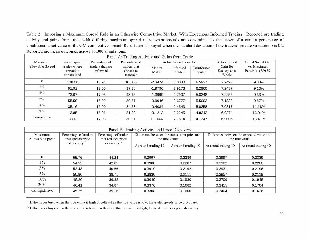
54

Table 2: Imposing a Maximum Spread Rule in an Otherwise Competitive Market, With Exogenous Informed Trading. Reported are trading activity and gains from trade with differing maximum spread rules, when spreads are constrained as the lesser of a certain percentage of conditional asset value or the GM competitive spread. Results are displayed when the standard deviation of the traders’ private valuation ρ is 0.2 Reported are mean outcomes across 10,000 simulations.

Panel A: Trading Activity and Gains from Trade Actual Social Gain for Maximum

Allowable Spread Percentage of trades where

spread is constrained

Percentage of traders that are

informed

Percentage of traders that choose to transact

Market Maker

Informed trader

Uninformed trader

Actual Social Gain for

Society as a Whole

Actual Social Gain vs. Maximum

Possible (7.9659)

0 100.00 16.94 100.00 -2.3474 3.0030 6.5937 7.2493 -9.03% 1% 91.91 17.05 97.38 -1.9796 2.9273 6.2960 7.2437 -9.10% 3% 73.07 17.05 93.15 -1.3999 2.7907 5.8348 7.2255 -9.33% 5% 55.59 16.99 89.51 -0.9946 2.6777 5.5002 7.1833 -9.87% 10% 35.16 16.90 84.53 -0.4084 2.4543 5.0358 7.0817 -11.18% 20% 13.85 16.96 81.29 -0.1213 2.2245 4.8342 6.9374 -13.01%

Competitive 0.00 17.03 80.91 0.0144 2.1514 4.7347 6.9005 -13.47%

Panel B: Trading Activity and Price Discovery Difference between the transaction price and

the true value Difference between the expected value and

the true value Maximum

Allowable Spread Percentage of traders

that speeds price discovery18

Percentage of traders that reduces price

discovery19 At round trading 10 At round trading 40 At round trading 10 At round trading 40

0 55.76 44.24 0.3997 0.2339 0.3997 0.2339 1% 54.52 42.85 0.3980 0.2287 0.3982 0.2288 3% 52.48 40.66 0.3919 0.2192 0.3931 0.2196 5% 50.80 38.71 0.3830 0.2111 0.3857 0.2119 10% 48.20 36.32 0.3649 0.1930 0.3709 0.1948 20% 46.41 34.87 0.3376 0.1682 0.3455 0.1704

Competitive 45.75 35.16 0.3308 0.1600 0.3404 0.1626 18 If the trader buys when the true value is high or sells when the true value is low, the trader speeds price discovery. 19 If the trader buys when the true value is low or sells when the true value is high, the trader reduces price discovery.

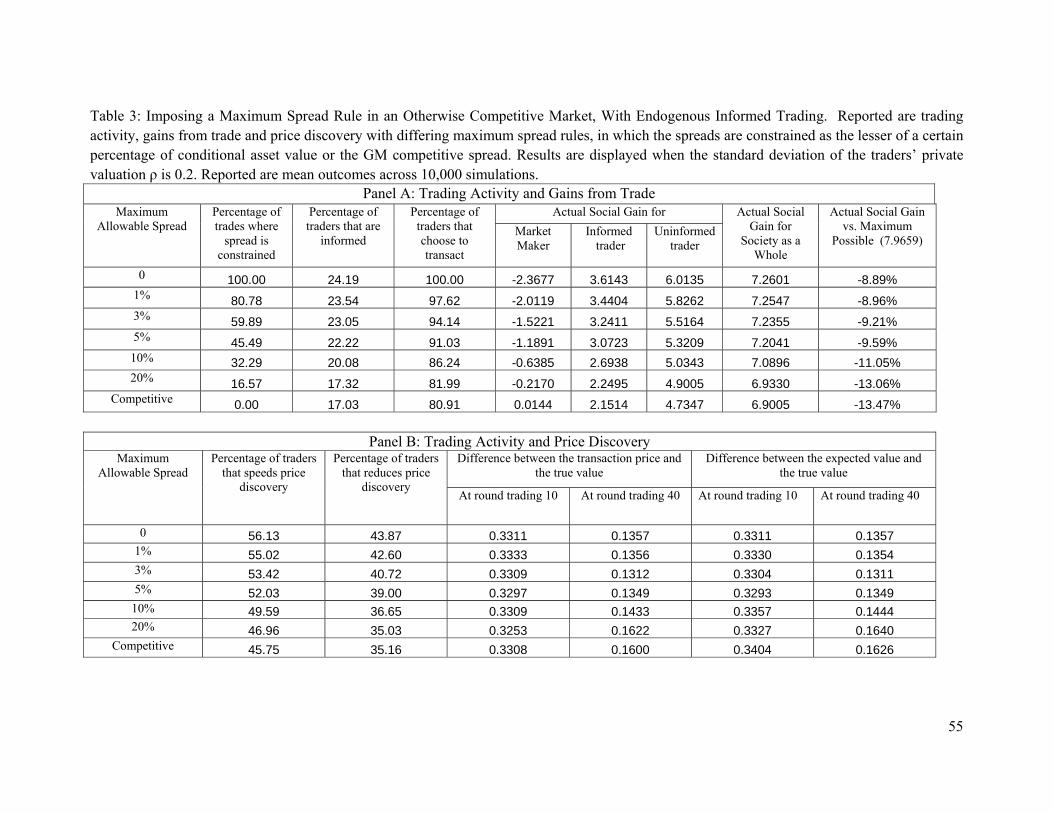
55

Table 3: Imposing a Maximum Spread Rule in an Otherwise Competitive Market, With Endogenous Informed Trading. Reported are trading activity, gains from trade and price discovery with differing maximum spread rules, in which the spreads are constrained as the lesser of a certain percentage of conditional asset value or the GM competitive spread. Results are displayed when the standard deviation of the traders’ private valuation ρ is 0.2. Reported are mean outcomes across 10,000 simulations.

Panel A: Trading Activity and Gains from Trade Actual Social Gain for Maximum

Allowable Spread Percentage of trades where

spread is constrained

Percentage of traders that are

informed

Percentage of traders that choose to transact

Market Maker

Informed trader

Uninformed trader

Actual Social Gain for

Society as a Whole

Actual Social Gain vs. Maximum

Possible (7.9659)

0 100.00 24.19 100.00 -2.3677 3.6143 6.0135 7.2601 -8.89% 1% 80.78 23.54 97.62 -2.0119 3.4404 5.8262 7.2547 -8.96% 3% 59.89 23.05 94.14 -1.5221 3.2411 5.5164 7.2355 -9.21% 5% 45.49 22.22 91.03 -1.1891 3.0723 5.3209 7.2041 -9.59% 10% 32.29 20.08 86.24 -0.6385 2.6938 5.0343 7.0896 -11.05% 20% 16.57 17.32 81.99 -0.2170 2.2495 4.9005 6.9330 -13.06%

Competitive 0.00 17.03 80.91 0.0144 2.1514 4.7347 6.9005 -13.47%

Panel B: Trading Activity and Price Discovery Difference between the transaction price and

the true value Difference between the expected value and

the true value Maximum

Allowable Spread Percentage of traders

that speeds price discovery

Percentage of traders that reduces price

discovery At round trading 10 At round trading 40 At round trading 10 At round trading 40

0 56.13 43.87 0.3311 0.1357 0.3311 0.1357 1% 55.02 42.60 0.3333 0.1356 0.3330 0.1354 3% 53.42 40.72 0.3309 0.1312 0.3304 0.1311 5% 52.03 39.00 0.3297 0.1349 0.3293 0.1349 10% 49.59 36.65 0.3309 0.1433 0.3357 0.1444 20% 46.96 35.03 0.3253 0.1622 0.3327 0.1640

Competitive 45.75 35.16 0.3308 0.1600 0.3404 0.1626

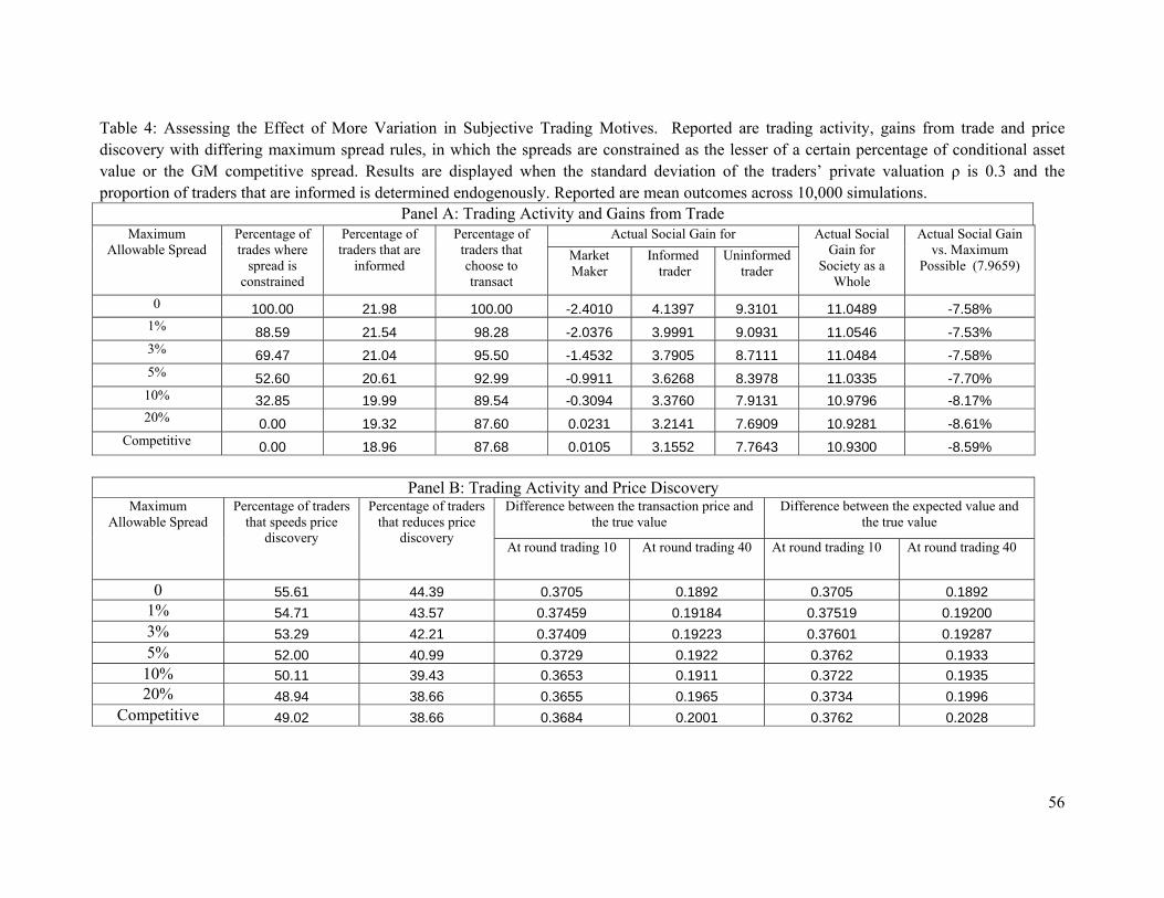
56

Table 4: Assessing the Effect of More Variation in Subjective Trading Motives. Reported are trading activity, gains from trade and price discovery with differing maximum spread rules, in which the spreads are constrained as the lesser of a certain percentage of conditional asset value or the GM competitive spread. Results are displayed when the standard deviation of the traders’ private valuation ρ is 0.3 and the proportion of traders that are informed is determined endogenously. Reported are mean outcomes across 10,000 simulations.

Panel A: Trading Activity and Gains from Trade Actual Social Gain for Maximum

Allowable Spread Percentage of trades where

spread is constrained

Percentage of traders that are

informed

Percentage of traders that choose to transact

Market Maker

Informed trader

Uninformed trader

Actual Social Gain for

Society as a Whole

Actual Social Gain vs. Maximum

Possible (7.9659)

0 100.00 21.98 100.00 -2.4010 4.1397 9.3101 11.0489 -7.58% 1% 88.59 21.54 98.28 -2.0376 3.9991 9.0931 11.0546 -7.53% 3% 69.47 21.04 95.50 -1.4532 3.7905 8.7111 11.0484 -7.58% 5% 52.60 20.61 92.99 -0.9911 3.6268 8.3978 11.0335 -7.70% 10% 32.85 19.99 89.54 -0.3094 3.3760 7.9131 10.9796 -8.17% 20% 0.00 19.32 87.60 0.0231 3.2141 7.6909 10.9281 -8.61%

Competitive 0.00 18.96 87.68 0.0105 3.1552 7.7643 10.9300 -8.59%

Panel B: Trading Activity and Price Discovery Difference between the transaction price and

the true value Difference between the expected value and

the true value Maximum

Allowable Spread Percentage of traders

that speeds price discovery

Percentage of traders that reduces price

discovery At round trading 10 At round trading 40 At round trading 10 At round trading 40

0 55.61 44.39 0.3705 0.1892 0.3705 0.1892 1% 54.71 43.57 0.37459 0.19184 0.37519 0.19200 3% 53.29 42.21 0.37409 0.19223 0.37601 0.19287 5% 52.00 40.99 0.3729 0.1922 0.3762 0.1933 10% 50.11 39.43 0.3653 0.1911 0.3722 0.1935 20% 48.94 38.66 0.3655 0.1965 0.3734 0.1996

Competitive 49.02 38.66 0.3684 0.2001 0.3762 0.2028

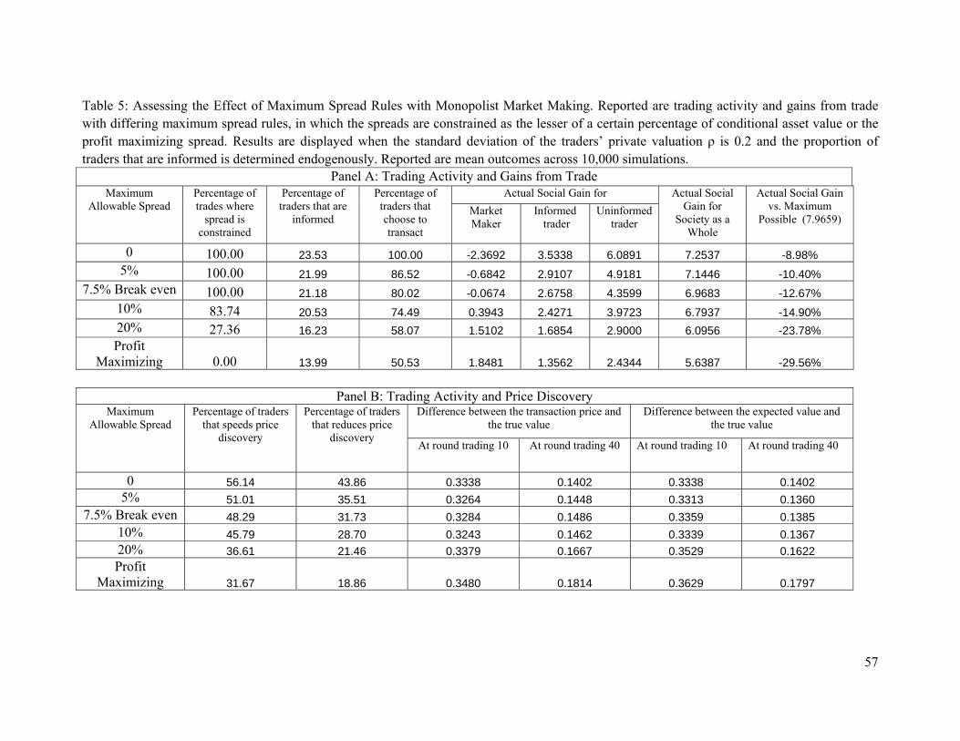
57

Table 5: Assessing the Effect of Maximum Spread Rules with Monopolist Market Making. Reported are trading activity and gains from trade with differing maximum spread rules, in which the spreads are constrained as the lesser of a certain percentage of conditional asset value or the profit maximizing spread. Results are displayed when the standard deviation of the traders’ private valuation ρ is 0.2 and the proportion of traders that are informed is determined endogenously. Reported are mean outcomes across 10,000 simulations.

Panel A: Trading Activity and Gains from Trade Actual Social Gain for Maximum

Allowable Spread Percentage of trades where

spread is constrained

Percentage of traders that are

informed

Percentage of traders that choose to transact

Market Maker

Informed trader

Uninformed trader

Actual Social Gain for

Society as a Whole

Actual Social Gain vs. Maximum

Possible (7.9659)

0 100.00 23.53 100.00 -2.3692 3.5338 6.0891 7.2537 -8.98% 5% 100.00 21.99 86.52 -0.6842 2.9107 4.9181 7.1446 -10.40%

7.5% Break even 100.00 21.18 80.02 -0.0674 2.6758 4.3599 6.9683 -12.67% 10% 83.74 20.53 74.49 0.3943 2.4271 3.9723 6.7937 -14.90% 20% 27.36 16.23 58.07 1.5102 1.6854 2.9000 6.0956 -23.78% Profit

Maximizing 0.00 13.99 50.53 1.8481 1.3562 2.4344 5.6387 -29.56%

Panel B: Trading Activity and Price Discovery Difference between the transaction price and

the true value Difference between the expected value and

the true value Maximum

Allowable Spread Percentage of traders

that speeds price discovery

Percentage of traders that reduces price

discovery At round trading 10 At round trading 40 At round trading 10 At round trading 40

0 56.14 43.86 0.3338 0.1402 0.3338 0.1402 5% 51.01 35.51 0.3264 0.1448 0.3313 0.1360

7.5% Break even 48.29 31.73 0.3284 0.1486 0.3359 0.1385 10% 45.79 28.70 0.3243 0.1462 0.3339 0.1367 20% 36.61 21.46 0.3379 0.1667 0.3529 0.1622 Profit

Maximizing 31.67 18.86 0.3480 0.1814 0.3629 0.1797

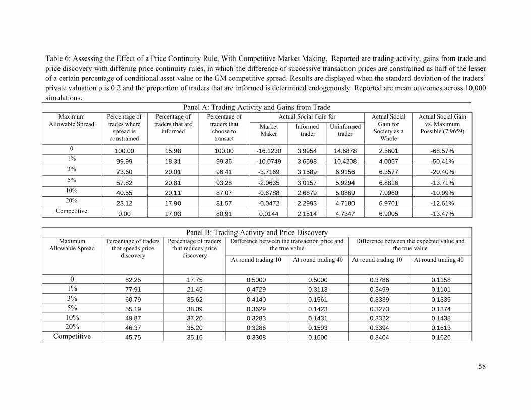
58

Table 6: Assessing the Effect of a Price Continuity Rule, With Competitive Market Making. Reported are trading activity, gains from trade and price discovery with differing price continuity rules, in which the difference of successive transaction prices are constrained as half of the lesser of a certain percentage of conditional asset value or the GM competitive spread. Results are displayed when the standard deviation of the traders’ private valuation ρ is 0.2 and the proportion of traders that are informed is determined endogenously. Reported are mean outcomes across 10,000 simulations.

Panel A: Trading Activity and Gains from Trade Actual Social Gain for Maximum

Allowable Spread Percentage of trades where

spread is constrained

Percentage of traders that are

informed

Percentage of traders that choose to transact

Market Maker

Informed trader

Uninformed trader

Actual Social Gain for

Society as a Whole

Actual Social Gain vs. Maximum

Possible (7.9659)

0 100.00 15.98 100.00 -16.1230 3.9954 14.6878 2.5601 -68.57% 1% 99.99 18.31 99.36 -10.0749 3.6598 10.4208 4.0057 -50.41% 3% 73.60 20.01 96.41 -3.7169 3.1589 6.9156 6.3577 -20.40% 5% 57.82 20.81 93.28 -2.0635 3.0157 5.9294 6.8816 -13.71% 10% 40.55 20.11 87.07 -0.6788 2.6879 5.0869 7.0960 -10.99% 20% 23.12 17.90 81.57 -0.0472 2.2993 4.7180 6.9701 -12.61%

Competitive 0.00 17.03 80.91 0.0144 2.1514 4.7347 6.9005 -13.47%

Panel B: Trading Activity and Price Discovery Difference between the transaction price and

the true value Difference between the expected value and

the true value Maximum

Allowable Spread Percentage of traders

that speeds price discovery

Percentage of traders that reduces price

discovery At round trading 10 At round trading 40 At round trading 10 At round trading 40

0 82.25 17.75 0.5000 0.5000 0.3786 0.1158 1% 77.91 21.45 0.4729 0.3113 0.3499 0.1101 3% 60.79 35.62 0.4140 0.1561 0.3339 0.1335 5% 55.19 38.09 0.3629 0.1423 0.3273 0.1374 10% 49.87 37.20 0.3283 0.1431 0.3322 0.1438 20% 46.37 35.20 0.3286 0.1593 0.3394 0.1613

Competitive 45.75 35.16 0.3308 0.1600 0.3404 0.1626