NBER WORKING PAPER SERIES

WHY ARE THE 2000S SO DIFFERENT FROM THE 1970S? A STRUCTURAL INTERPRETATIONOF CHANGES IN THE MACROECONOMIC EFFECTS OF OIL PRICES

Olivier J. BlanchardMarianna Riggi

Working Paper 15467http://www.nber.org/papers/w15467

NATIONAL BUREAU OF ECONOMIC RESEARCH1050 Massachusetts Avenue

Cambridge, MA 02138October 2009

We thank Efrem Castelnuovo, Giuseppe Ciccarone, Carlo Favero, Jordi Gali, Stefano Giglio, TommasoMonacelli, Luca Sala and Massimiliano Tancioni for helpful comments and suggestions. The viewsexpressed herein are those of the author(s) and do not necessarily reflect the views of the NationalBureau of Economic Research.

© 2009 by Olivier J. Blanchard and Marianna Riggi. All rights reserved. Short sections of text, notto exceed two paragraphs, may be quoted without explicit permission provided that full credit, including© notice, is given to the source.

Why are the 2000s so different from the 1970s? A structural interpretation of changes in themacroeconomic effects of oil pricesOlivier J. Blanchard and Marianna RiggiNBER Working Paper No. 15467October 2009JEL No. E3,E52

ABSTRACT

In the 1970s, large increases in the price of oil were associated with sharp decreases in output andlarge increases in inflation. In the 2000s, and at least until the end of 2007, even larger increases inthe price of oil were associated with much milder movements in output and inflation. Using a structuralVAR approach Blanchard and Gali (2007a) argued that this has reflected in large part a change inthe causal relation from the price of oil to output and inflation. In order to shed light on the possiblefactors behind the decrease in the macroeconomic effects of oil price shocks, we develop a new-Keynesianmodel, with imported oil used both in production and consumption, and we use a minimum distanceestimator that minimizes, over the set of structural parameters and for each of the two samples (preand post 1984), the distance between the empirical SVAR-based impulse response functions and thoseimplied by the model. Our results point to two relevant changes in the structure of the economy, whichhave modified the transmission mechanism of the oil shock: vanishing wage indexation and an improvementin the credibility of monetary policy. The relative importance of these two structural changes dependshowever on how we formalize the process of expectations formation by economic agents.

Olivier J. BlanchardInternational Monetary FundEconomic Counsellor and DirectorResearch Department700 19th Street, NWRm. 10-700Washington DC, 20431and NBERblanchar@mit.edu

Marianna RiggiUniversity of Rome "La Sapienza"marianna.riggi@uniroma1.it

Introduction

In the 1970s, large increases in the price of oil were associated with sharp decreases inoutput and large increases in inflation. In the 2000s, and at least until the end of 2007,even larger increases in the price of oil have been associated with much milder movementsin output and inflation1. Our goal in this paper is to look at the changes in the causalrelation from the price of oil to output and inflation in order to learn about the nature ofthe changes occurred in the structure of the economy.

Using a structural VAR approach, Blanchard and Gali (2007a) (BG in what follows)estimated impulse response functions (IRFs) for the United States, both for the pre-1984and the post-1984 periods, and concluded that the post-1984 effects of the price of oil oneither output or the price level were roughly equal to one-third of those for the pre-1984period.

They then explored informally the potential role of three factors in accounting for thechange: a smaller share of oil in production and consumption, lower real wage rigidity, andbetter monetary policy. Using a calibrated new-Keynesian model, they concluded that,in combination, these factors could potentially explain the change. They did not howeverestimate the model, nor –except for documenting the decrease in the share of oil inproduction and consumption– did they estimate the change in the relevant parameters.This is the natural next step, and this is what we do in this paper.

We write down a new-Keynesian model, with imported oil used both in productionand consumption and we then use a minimum distance estimator that minimizes, overthe set of structural parameters and for each of the two samples, the distance betweenthe empirical IRFs obtained by BG and those implied by the model. We reach two mainconclusions.

First, from a substantive point of view, our results indicate two relevant changes inthe structure of the economy which could have modified the transmission mechanismof the oil shocks: vanishing wage indexation and an improvement in the credibility ofmonetary policy. The identification of the relative importance of these two structuralchanges turns out to depend however on how we formalize the process of expectationsformation by agents. To capture the degree of anchoring of expectations, we use twospecifications, each of which strikes us as equally plausible. When inflation expectationsare partly affected by the current level of inflation, much of the difference between thetwo samples is attributed to changes occurred in the labor market and it can be tracedto a large decline in real wage rigidity, with a smaller role attributable to more effectivemonetary policy. Conversely, when households and firms partly base their expectations onlagged inflation the driving force behind the changes between the two periods is a moreeffective anchoring of inflation expectations, which we interpret as an improvement inmonetary policy credibility, with a smaller role for more flexible real wages. Under bothspecifications we find evidence of a slightly stronger interest rate reaction to expected

1While the large increase in the price of oil in 2008 may have played a role in the current crisis, it isclear that the sharp drop in output since then is due primarily to factors other than oil. Using data for2008 would give an undue large role to the price of oil in decreasing output. For this reason, we haveended our sample at the end of 2007.

2

inflation and of a decrease in nominal price rigidity over the post-1984 period, a factornot emphasized by BG. While the second formalization yields a slightly lower value forthe distance function, we find however that the difference between the two specificationsis not statistically significant.

Second, from a methodological point of view, our paper sheds light on the pros andcons of impulse response matching as a strategy of estimating model parameters. On theone hand, the advantage of identifying the parameters of the model from the IRFs to oilshock is that this shock is observable and can be directly and clearly identified in thedata. Hence, we trust the IRFs we ask the model to match. On the other hand, thisparticular shock only sheds light on some of the parameters, while being less informativeabout some others, and the fitting of only the set of IRFs related to oil shock does nothelp to disentangle between the relative role played by vanishing wage indexation and therole played by the improvement in the credibility of monetary policy.

Extending the minimum distance estimation to other well identified shocks, for whichthe two forces make a substantial difference, could help to disentangle their relative impor-tance. The natural candidates to look at are well identified demand side shocks. However,the empirical investigation extended to demand side shocks lies beyond the scope of thepresent paper and we leave it for future research.

The paper is organized as follows. Section 1 shows the IRFs from BG. Section 2presents the model. Section 3 discusses the results of estimation of the two benchmarkspecifications. Section 4 explores a number of extensions of the basic model. Section 5concludes.

3

1 Impulse responses

Figure 1 reproduces the impulse responses from BG which we shall try to fit with thestructural model. These are obtained from estimation of two structural VAR in six vari-ables, GDP, employment, the wage, the GDP deflator, the CPI, the nominal price ofoil, all in rates in change. Both VARs are estimated using quarterly data, the first overthe sample 1970:1-1983:4, the second over the sample 1984:1-2007:3. The identifying as-sumption is that innovations to the price of oil within the quarter are not affected byinnovations to the other variables.

The IRFs are shown for the first twenty quarters. The centered lines in each figuregive the estimated impulse responses of each variable, in level, to a positive shock to aprice of oil of 10%. The upper and lower lines give one-standard deviation bands, obtainedthrough Monte Carlo simulations. In all cases, the real price of oil shows a near-randomwalk response (not shown here), i.e. it jumps on impact, and then stays around a newplateau.

For our purposes, the IRFs in the figure have five major characteristics:

• Slowly building effects on activity and price variables in the two samples.

• Long lasting effects on all variables in the two samples.

• A smaller effect on GDP and employment in the second than in the first sample(roughly 1/3).

• A smaller effect on the GDP deflator and CPI in the second than in the first sample(roughly 1/3).

• No significant effect on nominal wages in the second sample, compared to a strongand significant effect in the first sample.

2 A model

To interpret these IRFs and recover structural parameters, we develop a new-Keynesianmodel. The model is standard, except for four extensions, each needed for our purposes.

• We allow for the use of oil as an input in both production and consumption. Weassume that the country is an oil importer, and take the real price of oil (in termsof domestic goods) as exogenous.

• We allow for habit formation in consumption. This is done in order to capture thefirst characteristic of the data listed in the previous section, namely the slow adjust-ment of output and employment over time. In the model, output is determined bydemand, and equal to consumption, and habit formation leads to a slow adjustmentof consumption.

4

• We allow for real wage rigidity, one of the potential factors emphasized by BG.We formalize it as a slow adjustment of the real wage at which workers are willingto work to their marginal rate of substitution. That real wage rigidity may havedecreased over time seems plausible, as weakening unions, increasing competitionand declining minimum wage have made the structure of labor compensation muchmore flexible in the 2000s than it was in the 1970s.

• To capture the notion of policy credibility, we allow agents’ inflation expectationsto depend directly on current or past inflation. The smaller the dependence on cur-rent or past inflation, the better anchored are inflation expectations, and the morefavorable is the trade-off between inflation and output. That inflation expectationsmay have become better anchored over time also strikes us as plausible. BG providedirect evidence of a decrease in the response of expected inflation to the oil priceshock since the mid-1980s, while the strength of the response of the nominal interestrate has not changed much across sample periods. Variations in the dynamics ofexpectations play a key role in the "good policy" hypothesis of the Great Moder-ation (Clarida, Gali and Gertler (2000), Lubik and Schorfheide (2004), Boivin andGiannoni (2002 and 2006), Castelnuovo and Surico (forthcoming), and Canova andGambetti (2009 and forthcoming) for a dissenting view)

The rest of the section presents only the implied log-linearized equations, leaving thefull derivation to the appendix. Lower case letters represent deviations from steady state,lower case letters with a hat are proportional deviations from steady state.

2.1 Oil in production and in consumption

Production is characterized by a Cobb-Douglas production function in labor and oil:

qt = αn nt + αm mt (1)

where qt is (gross) domestic product, nt is labor, mt is the quantity of imported oil usedin production, αn + αm ≤ 1. Technological progress does not affect the IRF to oil andcan thus be ignored here.

Consumption is characterized by a Cobb-Douglas consumption function in output andoil:

ct = (1− χ)cq,t + χcm,t (2)

where ct is consumption, cq,t is consumption of the domestically produced good, cm,t isconsumption of imported oil.

In this environment, it is important to distinguish between two prices, the price ofdomestic output pq,t and the price of consumption pc,t. Let pm,t be the price of oil, andst ≡ pm,t−pq,t be the real price of oil, which is assumed to follow a first order autoregressiveprocess. From the definition of consumption, the relation between the consumption priceand the domestic output price is given by:

pc,t = pq,t + χ st (3)

5

The important parameters for our purposes are αm and χ, the share of oil in productionand in consumption.

2.2 Households

The behavior of households is characterized by two equations. The first one characterizesconsumption:

ct =h

1 + hct−1 +

1

1 + hEtct+1 −

(1− h)

(1 + h) σ

(it − πec,t+1 + log β

)(4)

Consumption depends on itself lagged, itself expected, and on the real interest rate interms of consumption. The parameter σ is the household risk aversion coefficient; togetherwith h, it determines the response of consumption to the real interest rate. The parameterh ∈ [0, 1) captures habit formation (the utility of consumption depends on C − hC(−1),where C is current consumption, and C(−1) is lagged aggregate consumption). The higherthe value of h, the slower the adjustment of the consumption; when h = 0, the relationreduces to the usual Euler equation.

The second equation characterizes labor supply, or equivalently, the real consumptionwage at which workers are willing to work (the “supply wage”):

wt − pc,t = γ (wt−1 − pc,t−1) + (1− γ)

{φnt +

σ

1− h[ct − hct−1]

}(5)

where wt denotes the nominal wage. The supply wage depends on itself lagged, and onthe marginal rate of substitution. The marginal rate of substitution depends in turnon employment, with elasticity φ, where φ is the inverse of the Frisch elasticity, and onct − hct−1, with elasticity σ/(1 − h). The parameter γ ∈ [0, 1) captures the extent ofreal wage rigidity, which is needed in order to generate a meaningful trade-off betweenstabilization of inflation and the welfare relevant output gap (Blanchard and Gali, 2007b).When γ = 0, the supply wage is equal to the marginal rate of substitution. The higherthe value of γ, the higher the degree of real wage rigidity.

2.3 Firms

Domestic goods are imperfect substitutes in consumption, and firms are thus monopolisticcompetitors. Given the production function, cost minimization implies that the firms’demand for oil is given by:

mt = −µt − st + qt (6)

where µt is the log deviation of the price markup, Mt. Using this expression to eliminatemt in the production function gives a reduced-form production function:

qt =1

1− αm(αnnt − αmst − αmµpt ) (7)

Given employment, output is a decreasing function of the real price of oil.

6

Combining the cost minimization conditions for oil and for labor with the aggregateproduction function yields the following factor price frontier:

(1− αm) (wt − pc,t) + (αm + (1− αm)χ) st + (1− αn − αm) nt + µt = 0 (8)

Given productivity, an increase in the real price of oil must lead to one or more of thefollowing adjustments: (i) a lower consumption wage, (ii) lower employment, (iii) a lowermarkup.

This equation defines the real consumption wage consistent with a given markup setby firms; we can think of it as giving us the “demand wage” as a function of employment.This will be useful below.

Firms are assumed to set prices à la Calvo (1983), an assumption which yields thefollowing log-linearized equation for domestic output price inflation (domestic inflationfor short):

πq,t = βπeq,t+1 − λp µt (9)

where λp ≡ [(1 − θ)(1 − βθ)/θ][(αm + αn)/(1 + (1 − αm − αn)(ǫ − 1))], θ denotes thefraction of firms that leave prices unchanged during a given period, β is the discountfactor of households and ǫ is the elasticity of substitution between domestic goods inconsumption.

2.4 Consumption, output, employment, and GDP

The condition that trade be balanced (as oil is imported) gives us a relation betweenconsumption and output:

ct = qt − χst − ηµt (10)

where η ≡ αm/(M− αm).Using the reduced-form production function (7) gives a relation between consumption

and employment:

ct =αn

1− αmnt −

(χ+

αm1− αm

)st +

(η −

αm1− αm

)µt (11)

The characterization of the equilibrium does not require to introduce either value addedor the value added deflator. But these are needed to compare the implications of themodel to the data.

The value added deflator py,t is implicitly defined by pq,t = (1 − αm)py,t + αm pm,t.Rearranging terms gives:

py,t = pq,t −αm

1− αmst (12)

thus implying a negative effect of the real price of oil on the GDP deflator, given domesticoutput prices.

The definition of value added, combined with the demand for oil, yields the followingrelation between GDP and gross output:

yt = qt +αm

1− αmst + η µt (13)

7

2.5 Monetary policy

Monetary policy is characterized by a Taylor rule in which the interest rate responds tothe deviation of expected CPI inflation from a zero target inflation:

i = − log β + φπ(Etπc,t+1) (14)

In order to analyze to what extent anti-inflation credibility may have played a role forthe decrease in the dynamic effects of oil shocks, we depart from the standard forwardlooking inflation expectations for agents other than the central bank, and we explore twoapparently similar, and equally plausible ex-ante specifications. In the first case, we allowexpectations to depend directly on current inflation; in the second, we allow expectationsto depend directly on inflation in the previous quarter. In both cases we interpret theparameter λ ∈ [0, 1] as capturing the quality of monetary policy. The lower λ, the lesscredible monetary policy, the worse the anchoring of inflation expectations and the worsethe implied trade-off between inflation and output. Both model specifications capture theidea that, when credibility is low, the central bank is unable to establish an anchor forinflation expectations, which thus turn out to be strongly connected with actual inflationdynamics.

i) In the first specification we assume that economic agents form expectations of inflationaccording to:

πec,t+1 = (1− λ) πc,t + λEtπc,t+1 (15)

πeq,t+1 = (1− λ)πq,t + λEtπq,t+1 (16)

ii) In the second specification we assume that economic agents form expectations ofinflation according to:

πec,t+1 = (1− λ) πc,t−1 + λEtπc,t+1 (17)

πeq,t+1 = (1− λ) πq,t−1 + λEtπq,t+1 (18)

The difference between the two specifications seems minor. Yet, as we shall show, itgives rise to very different interpretations of the data.

8

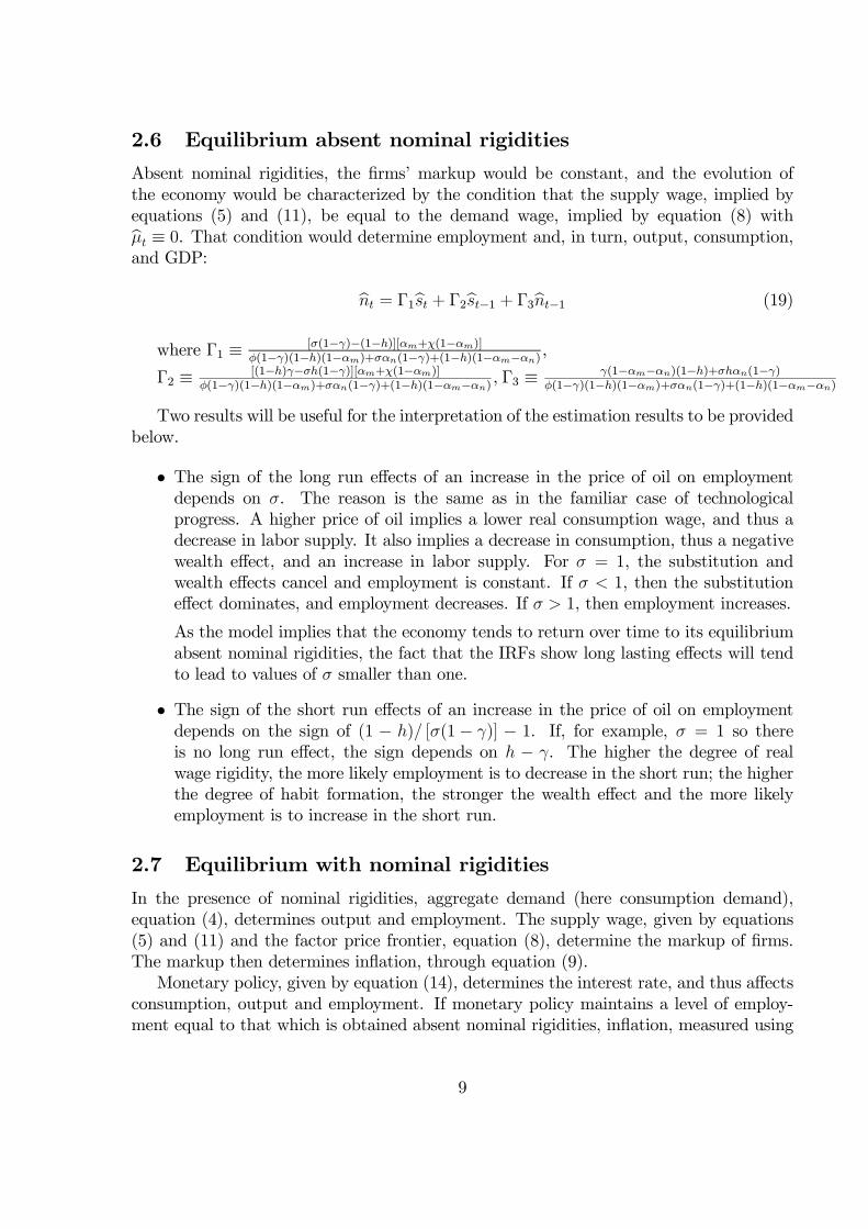
2.6 Equilibrium absent nominal rigidities

Absent nominal rigidities, the firms’ markup would be constant, and the evolution ofthe economy would be characterized by the condition that the supply wage, implied byequations (5) and (11), be equal to the demand wage, implied by equation (8) withµt ≡ 0. That condition would determine employment and, in turn, output, consumption,and GDP:

nt = Γ1st + Γ2st−1 + Γ3nt−1 (19)

where Γ1 ≡[σ(1−γ)−(1−h)][αm+χ(1−αm)]

φ(1−γ)(1−h)(1−αm)+σαn(1−γ)+(1−h)(1−αm−αn),

Γ2 ≡[(1−h)γ−σh(1−γ)][αm+χ(1−αm)]

φ(1−γ)(1−h)(1−αm)+σαn(1−γ)+(1−h)(1−αm−αn), Γ3 ≡

γ(1−αm−αn)(1−h)+σhαn(1−γ)φ(1−γ)(1−h)(1−αm)+σαn(1−γ)+(1−h)(1−αm−αn)

Two results will be useful for the interpretation of the estimation results to be providedbelow.

• The sign of the long run effects of an increase in the price of oil on employmentdepends on σ. The reason is the same as in the familiar case of technologicalprogress. A higher price of oil implies a lower real consumption wage, and thus adecrease in labor supply. It also implies a decrease in consumption, thus a negativewealth effect, and an increase in labor supply. For σ = 1, the substitution andwealth effects cancel and employment is constant. If σ < 1, then the substitutioneffect dominates, and employment decreases. If σ > 1, then employment increases.

As the model implies that the economy tends to return over time to its equilibriumabsent nominal rigidities, the fact that the IRFs show long lasting effects will tendto lead to values of σ smaller than one.

• The sign of the short run effects of an increase in the price of oil on employmentdepends on the sign of (1 − h)/ [σ(1− γ)] − 1. If, for example, σ = 1 so thereis no long run effect, the sign depends on h − γ. The higher the degree of realwage rigidity, the more likely employment is to decrease in the short run; the higherthe degree of habit formation, the stronger the wealth effect and the more likelyemployment is to increase in the short run.

2.7 Equilibrium with nominal rigidities

In the presence of nominal rigidities, aggregate demand (here consumption demand),equation (4), determines output and employment. The supply wage, given by equations(5) and (11) and the factor price frontier, equation (8), determine the markup of firms.The markup then determines inflation, through equation (9).

Monetary policy, given by equation (14), determines the interest rate, and thus affectsconsumption, output and employment. If monetary policy maintains a level of employ-ment equal to that which is obtained absent nominal rigidities, inflation, measured using

9

the output price, is constant. If it tries to maintain higher employment, then inflation ishigher.

The coefficients associated with nominal rigidities and with monetary policy play thefollowing role. A lower value of θ (i.e. lower nominal rigidity) leads to a stronger effectof a given decrease in the markup on inflation. Thus, for a given policy rule, it leads to alarger initial increase in inflation and a larger initial decline in output.

A higher value of φπ leads to a smaller increase in inflation but at the expense of alarger decrease in output.

Under both specifications for inflation expectations, the lower λ, the worse the trade-off between stabilization of quantities and stabilization of prices in response to oil priceshocks. Credibility gains, captured by a higher λ, improve the trade-off facing policy-makers and make it possible to have a smaller impact of a given oil price increase on bothinflation and output.

Furthermore, as shown in figure 2, the shape of the dynamic effects are notably differentacross the two model specifications.

When we assume that people form their expectations according to equations (15) and(16), the response of inflation expectations is stronger the lower is λ, but its dynamics arenot affected: the largest increase occurs at the start, going subsequently to zero.

On the contrary, when we consider a backward looking behavior according to equations(17) and (18), not only the magnitude but also the shape of the inflation expectations’response is affected. In this case, the lower is λ, the more hump-shaped the inflationexpectations response.

3 Estimation of the Benchmark

Call X the vector of the 13 parameters of the model. Let Ψ(X) be the set of impulseresponses of pc,t, py,t, wt, yt and nt over the first 20 quarters to an increase in the price of

oil implied by X, and let Ψ be the estimated IRFs from BG presented in Figure 1. Theminimum distance estimator of X we use is given by2

X = argmin[Ψ−Ψ(X)]′D−1[Ψ−Ψ(X)] (20)

where D is a diagonal matrix, with the sample variances of the Ψ along the diagonal (sothat the more tightly estimated IRFs get more weight in estimation).

X is given by X ≡ (αn, αm, β, χ, φ, σ, ǫ, h, γ, θ, φπ, λ, ρ). We estimate X separately foreach of the two samples, 1970:1 to 1983:4, and 1984:1 to 2007:3.

Estimating all 13 parameters would be asking too much of the data. Thus, we choosea number of coefficients a priori:

The coefficients capturing the role of oil in production and in consumption, αm andχ, can be constructed directly. Following the computations in BG, we choose αm = 1.5%

2Impulse response matching, as a way of estimating model parameters, has been recently put forwardby Christiano at al (2005).

10

and χ = 2.3% for the first sample, αm = 1.2% and χ = 1.7% for the second sample. Theway in which these shares affect the outcome is through the expression αm + (1− αm)χ(as can be seen by looking at the term in s in the factor price frontier, (8)). So thesenumbers imply that, other things equal, the effect of a given increase in the price of oil inthe second sample is only 3/4 of the effect in first sample.

We assume that, in the short run, firms have enough capital capacity that they operateunder constant returns to labor and oil, so αn = 1− αm. We calibrate the autoregressiveparameter of the oil shock ρ = 0.999, in order to have the price of oil being very closeto random walk, as it is in the data, while retaining stationarity to have a determinatesteady state.

With respect to preferences, we assume β = 0.99, ǫ = 6.0 (so that the desired markupof firms over marginal cost is 20%), and a Frisch elasticity φ = 1.0. Given the long lastingeffects of the price of oil in the IRFs, we do not impose long-run neutrality (σ = 1), andallow for σ to be estimated. As both consumption and labor supply decisions depend oninteractions of σ and h, and we let the data determine σ, we do the same for h.

This leaves us with six parameters to be estimated, σ and h for preferences, γ for realwage rigidity, θ for nominal price rigidity and φπ and λ for monetary policy.

3.1 Benchmark parameters

The results of the estimations of the benchmark under specification i and ii are shown inTable 1 and 2, respectively. The last column gives the minimized value of the distancefunction. The implied and actual IRFs under the model specification (i) and under themodel specification (ii) are shown in Figure 3a and 3b respectively3. Standard errors arereported in parenthesis.

Table 1. Benchmark Estimated Parameters

specification (i)

σ h γ θ φπ λDistance

Function

Pre-19840.111(0.062)

0.971(0.049)

0.968(0.125)

0.678(0.101)

2.887(1.395)

0.987(0.289)

115.0314

Post-19840.145(0.043)

0.898(0.531)

0.033(0.056)

0.134(0.027)

3.785(1.625)

1.000(0.593)

65.5805

3Clarida, Gali and Gertler (2000) have highlighted the role of indeterminate equilibriums in the pre-1979 period. We pursue an alternative line of explanation here, which does not rely on sunspot fluctuationsin the pre-1984 sample. Thus, in the numerical minimization of (20) we consider only the combinationsof the structural parameters such that the model satifies Blanchard and Kahn (1980) conditions. Besides,we impose restrictions on the sign and the magnitude of the parameters which are consistent with theirmeaning.

11

Table 2. Benchmark Estimated Parameters

specification (ii)

σ h γ θ φπ λDistance

Function

Pre-19840.100∗

(0.002)0.911(0.483)

0.284(0.378)

0.231(0.154)

2.038(0.736)

0.103(0.505)

84.1481

Post-19840.152(0.046)

0.897(0.029)

0.094(0.116)

0.126(0.016)

3.937(0.479)

0.970(0.078)

65.2519

Notes: Standard errors in parentheses. A star denotes that the estimate reaches the lower

bound imposed in estimation.

For the first sample the minimized value of the distance function under specification(ii) is somewhat lower than under specification (i). This raises the question of whetherwe can reject the first specification relative to the second. However, the distribution ofthe distance function is unknown (as we are not using the efficient weighting matrix, wecannot use the Hansen’s J statistic). In order to compare the measures of goodness of fitbetween the two models, we thus use a bootstrap methodology to compute the empiricalprobability density function of the statistic given by the difference between the goodness offit of the two model specifications4. The empirical density function is a bell curve centeredat zero. The difference between the goodness of fit of the two model specifications is notstatistically significant at the 95% confidence level: we conclude that the better fit of thesecond specification is not significantly better. Thus, in the rest of the paper, we treatthe two specifications in parallel.

Tables 1 and 2 and Figures 2a and 2b then suggest the following conclusions:

• Regardless of the ex ante assumption on the way people form their expectations, themodel provides a good fit of the impulse responses in both samples. The impliedIRFs are typically within the one-standard deviation bands. The lower value of thedistance function obtained for the pre-1984 sample under model specification (ii) isdue to an excellent fit of the price and wage dynamics, whereas the larger decreasein quantities is captured less well by the model.

• While the estimates for the post-1984 sample are remarkably stable across the modelspecifications, for the pre-1984 sample there are different sets of parameters thatwork nearly equally well across the two equally plausible ex-ante specifications.

Under the model specification (i), the main difference between the two samples isattributed to a dramatic decline in the degree of real wage rigidity γ, from 0.968 in

4We generate bootstrap residuals by randomly drawing with replacement from the set of estimatedresiduals. We construct bootstrap time-series by adding the randomly resampled residuals to the predictedvalues and re-estimate the parameters from the fictitious data. On the basis of these parameters, wecompute the statistic of interest.

12

the first sample, to 0.03 in the second. The estimated value of λ does not suggestan important role for the improvement in monetary policy credibility.

Using the terminology often used by central banks, this can be described as strong“second-round” effects pre-1984, and weak or non existent ones post-1984. Facedwith similar initial increases in the CPI (the “first round” effects), and for givenemployment, workers in the 1970s asked for and obtained increases in nominal wages,which then led to higher prices, confronting the central bank with a worse trade-offbetween activity and inflation. In the 2000s, the same initial increases in the CPIhave not led to increases in nominal wages, and thus to further increases in prices.

When people are assumed to form their expectations according to the model speci-fication (ii), although the estimated value of γ is still higher in the pre-1984 than inthe post-1984 sample, the crucial role in explaining the different effects of oil priceshocks is played by a strong improvement in the anchoring of inflation expectations,i.e., by an increase in the estimated value of λ, which we interpret as an increase incentral bank credibility.

In the pre-1984 sample, after the oil shock, the adjustment of inflation expectationsis slow, but increases over time. Conversely, in the post-1984 sample inflation ex-pectations rise at the start but people anticipate that inflation will decrease lateron. The central bank’s inability to anchor expectations, coupled with a milder reac-tion of the nominal interest rate, makes monetary policy much less effective in thepre-1984 sample than in the post-1984 one, thus leading to greater macroeconomicvolatility.

• The values of σ and h are fairly similar across the two samples and across the modelspecifications. This is good news, as we would hope preferences to be relativelystable over time. The low value of σ implies a large negative long-run effect of anincrease in the price of oil on employment.

• Under both specifications, the degree of nominal price rigidity θ is estimated to havedecreased over time. This runs against our (and we would guess, most economists’)priors. First, as inflation has decreased over time, we would expect price setters tochange prices less often. Secondly, a number of recent papers find a flatter Phillipscurve characterizing the Great Moderation,which would suggest a slower price ad-justment in the post 1984 period. If indeed present, the lower degree of nominalprice rigidities may come as a consequence of the higher competition experienced inthe last decades, which has probably forced firms to adjust prices more often.

In the pre-1984 sample, model specification (i) is associated with a higher estimateddegree of price stickiness (θ = 0.678) than the model specification (ii) (θ = 0.231).As a matter of fact, the estimated value of θ is linked to the estimated value of thedegree of real wage rigidity γ. The reason is as follows. The estimated high degreeof real wage rigidity in the first sample implies a large negative initial effect on thenatural level of employment (the level that would obtain in the absence of nominalrigidities). Given actual employment and for a given degree of nominal rigidity, this

13

would lead to even more inflation in the first sample than is actually observed inthe data. Thus, the model estimates θ, the degree of nominal rigidity, to be higherin the first sample than in the second one, especially under the model specification(i).

• The weight on expected inflation in the Taylor rule is consistent across specifications,and it is estimated to be higher in the second sample than in the first one (3.785versus 2.887 under the first specification, and 3.937 versus 2.037 under the secondspecification). This higher weight cannot however, by itself, explain the smallereffects on both activity and inflation: a stronger anti-inflationary stance can reducethe volatility of inflation but increase that of GDP.

Our two benchmark estimates point to two relevant changes in the structure of theeconomy which have modified the mechanism through which oil price shocks propagatein the economy: a more flexible labor market and a more credible monetary policy.

Some findings are consistent across model specifications: a somewhat stronger interestrate response to variations in expected inflation, a decrease in real wage and nominalprice rigidity (although the magnitude of such decreases is very different across the twomodel specifications) and some role attributed to the smaller share of oil in productionand consumption. However, it is hard to identify which of the two structural changesis the major factor behind the smaller effects of oil price shocks in the 2000s than inthe 1970s. The interpretations of the macroeconomic changes in the effects of oil pricesprovided by the two model specifications are very different.

Estimation of the benchmark under the model specification (i) denies a role for theanchoring of expectations and points to changes in the labor market occurred in term of anincrease of real wage flexibility as the main driving force behind the observed change in theeconomy’s response to the oil price shock. Conversely, estimation of the benchmark underthe second specification identifies the source of the milder reaction of prices and quantitiesin monetary policy, which has become more stabilizing, as a result of a greater effectivenessin the anchoring of expectations coupled with a stronger interest rate reaction.

The rest of our paper explores the robustness of these conclusions.

4 Extensions

4.1 Alternative estimated IRFs

The benchmark estimated parameters shown in tables 1 and 2 are obtained using anunderlying VAR estimated with variables in rates of change. Estimating everything in firstdifferences could force long run effects on value added and employment. We thus explorethe effects on the benchmark estimated parameters of an alternative VAR specification,which uses rates of change for prices and wage and log-deviations from a linear trend forthe quantity variables. Figure 4 reproduces the IRFs obtained from the estimation of thelevel/growth specification of the VAR. The results of the structural estimation using suchspecification are shown in table 3 for the model specification (i) and in table 4 for the

14

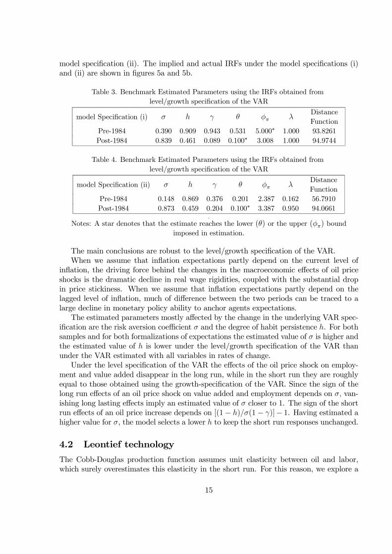
model specification (ii). The implied and actual IRFs under the model specifications (i)and (ii) are shown in figures 5a and 5b.

Table 3. Benchmark Estimated Parameters using the IRFs obtained from

level/growth specification of the VAR

model Specification (i) σ h γ θ φπ λDistance

Function

Pre-1984 0.390 0.909 0.943 0.531 5.000∗ 1.000 93.8261

Post-1984 0.839 0.461 0.089 0.100∗ 3.008 1.000 94.9744

Table 4. Benchmark Estimated Parameters using the IRFs obtained from

level/growth specification of the VAR

model Specification (ii) σ h γ θ φπ λDistance

Function

Pre-1984 0.148 0.869 0.376 0.201 2.387 0.162 56.7910

Post-1984 0.873 0.459 0.204 0.100∗ 3.387 0.950 94.0661.

Notes: A star denotes that the estimate reaches the lower (θ) or the upper (φπ) bound

imposed in estimation.

The main conclusions are robust to the level/growth specification of the VAR.When we assume that inflation expectations partly depend on the current level of

inflation, the driving force behind the changes in the macroeconomic effects of oil priceshocks is the dramatic decline in real wage rigidities, coupled with the substantial dropin price stickiness. When we assume that inflation expectations partly depend on thelagged level of inflation, much of difference between the two periods can be traced to alarge decline in monetary policy ability to anchor agents expectations.

The estimated parameters mostly affected by the change in the underlying VAR spec-ification are the risk aversion coefficient σ and the degree of habit persistence h. For bothsamples and for both formalizations of expectations the estimated value of σ is higher andthe estimated value of h is lower under the level/growth specification of the VAR thanunder the VAR estimated with all variables in rates of change.

Under the level specification of the VAR the effects of the oil price shock on employ-ment and value added disappear in the long run, while in the short run they are roughlyequal to those obtained using the growth-specification of the VAR. Since the sign of thelong run effects of an oil price shock on value added and employment depends on σ, van-ishing long lasting effects imply an estimated value of σ closer to 1. The sign of the shortrun effects of an oil price increase depends on [(1− h)/σ(1− γ)]− 1. Having estimated ahigher value for σ, the model selects a lower h to keep the short run responses unchanged.

4.2 Leontief technology

The Cobb-Douglas production function assumes unit elasticity between oil and labor,which surely overestimates this elasticity in the short run. For this reason, we explore a

15

Leontief model, where labor and oil are combined in fixed proportions. The productionfunction is given by:

qt = nt = mt (21)

Consumption is still characterized by the Cobb-Douglas function in output and oil(2) and the relation between the consumption price and the domestic output price is stillgiven by equation (3). The Euler equation (4) and the supply wage (5) hence continue tocharacterize the behavior of households. Real marginal cost is given by:

mct = αn (wt − pq,t) + αmst (22)

As before, we follow the formalism proposed in Calvo (1983), and assume that in eachperiod a measure (1− θ) of firms reset their prices. This yields the following equation fordomestic inflation:

πq,t = βπeq,t+1 +(1− θ) (1− βθ)

θmct (23)

With balanced trade the following relation must hold:

ct = qt −

(χ+

αmM− αm

)st (24)

The specification of technology implies a relation between value added and gross out-put:

yt = qt (25)

while the value added deflator is given by:

py,t = wt (26)

Inflation expectations are still given by (15) and (16) under the model specification(i) and by (17) and (18) under the model specification ii)

Tables 5 and 6 report the estimated parameters5. Figures 6a and 6b display estimatedand implied IRFs.

Table 5. Estimated Parameters under Leontief technology. Specification (i)

σ h γ θ φπ λDistance

Function

Pre-1984 0.637 0.870 0.991 0.947 3.113 1.000 133.6951

Post-1984 0.100∗ 0.937 0.001∗ 0.662 3.430 1.000 38.5495

5Parameters are estimated using the benchmark VAR.

16

Table 6 Estimated Parameters under Leontief technology. Specification (ii)

σ h γ θ φπ λDistance

Function

Pre-1984 0.100∗ 0.919 0.265 0.485 2.037 0.000 72.6659

Post-1984 0.100∗ 0.926 0.094 0.737 3.387 0.677 34.9838

Notes: A star denotes that the estimate reaches the lower bound imposed in estimation.

The main conclusions are robust to changes in the specification of technology. Thevanishing real wage rigidities are the driving force behind the change in the effects of oilshocks under the model specification (i). The improvement in the anchoring of expecta-tions is the major force leading to the decline in macroeconomic volatility after the oilshock under the model specification (ii).

The degree of price stickiness is however higher in both samples and for both modelspecification than under the Cobb Douglas specification. The reason is as follows. Sincethere is no substitution of labor for oil in response to the oil price increase, the Leontieftechnology produces initial larger effects on both quantities and prices. As lower nominalrigidity implies larger initial rises in inflation and larger initial drops in output, through astronger reaction of inflation to a given decrease in the markup, the Leontief technologyrequires more price stickiness to fit the data than the Cobb Douglas technology.

It is worth noting that, taking into account the value attained by the distance function,in the second sample the model with Leontief Technology outperforms that with CobbDouglas technology. In the pre 1984 sample the two models are nearly equivalent inproviding the IRFs matches.

4.3 Variable desired markups

Rotemberg and Woodford (1996) have argued that another effect was at work behindthe size of the observed effects of oil price shocks in the 1970s, namely, an endogenousincrease in the firms’ markups leading to a larger decrease in output. We capture theidea that the change in the relevance of the oil price as a source of economic fluctuationscould have been caused by variations in the degree of the countercyclicality of markups byspecifying the desired markup as a function of the real price of oil s. The endogenous risein the desired markup significantly increases the predicted effects of an oil price shock onboth quantities and prices. As shown in Appendix b, this assumption modifies domesticinflation (9) which now contains an additive cost push shock:

πq,t = β Et{πq,t+1} − λpµt + λpφε

ε− 1st (27)

where φε ∈ [0, 1) is a measure of the sensitivity of the desired markup to changes inthe real price of oil.

Tables 7 and 8 shows the results of estimation, conditional on different values of φε6.

Depending on the sample and the specification, the distance function is minimized for

6Parameters are estimated using the benchmark VAR.

17

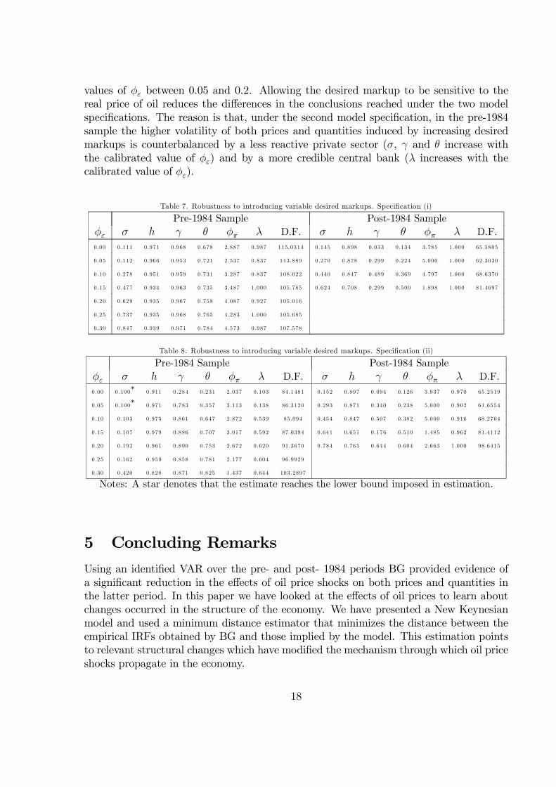
values of φε between 0.05 and 0.2. Allowing the desired markup to be sensitive to thereal price of oil reduces the differences in the conclusions reached under the two modelspecifications. The reason is that, under the second model specification, in the pre-1984sample the higher volatility of both prices and quantities induced by increasing desiredmarkups is counterbalanced by a less reactive private sector (σ, γ and θ increase withthe calibrated value of φε) and by a more credible central bank (λ increases with thecalibrated value of φε).

Table 7. Robustness to introducing variable desired markups. Specification (i)

Pre-1984 Sample Post-1984 Sample

φε σ h γ θ φπ λ D.F. σ h γ θ φπ λ D.F.

0 .00 0.111 0.971 0.968 0 .678 2 .887 0 .987 115.0314 0 .145 0 .898 0.033 0.134 3.785 1.000 65.5805

0 .05 0.112 0.966 0.953 0 .721 2 .537 0 .837 113 .889 0 .270 0 .878 0.299 0.224 5.000 1.000 62.3030

0 .10 0.278 0.951 0.959 0 .731 3 .287 0 .837 108 .022 0 .440 0 .847 0.489 0.369 4.797 1.000 68.6370

0 .15 0.477 0.934 0.963 0 .735 3 .487 1 .000 105 .785 0 .624 0 .708 0.299 0.500 1.898 1.000 81.4697

0 .20 0.629 0.935 0.967 0 .758 4 .087 0 .927 105 .016

0 .25 0.737 0.935 0.968 0 .765 4 .283 1 .000 105 .685

0 .30 0.847 0.939 0.971 0 .784 4 .573 0 .987 107 .578

Table 8. Robustness to introducing variable desired markups. Specification (ii)

Pre-1984 Sample Post-1984 Sample

φε σ h γ θ φπ λ D.F. σ h γ θ φπ λ D.F.

0.00 0.100∗

0 .911 0 .284 0 .231 2.037 0.103 84 .1481 0.152 0.897 0.094 0.126 3.937 0 .970 65.2519

0.05 0.100∗

0 .971 0 .783 0 .357 3.113 0.138 86 .3120 0.293 0.871 0.340 0.238 5.000 0 .902 61.6554

0.10 0.103 0 .975 0 .861 0 .647 2.872 0.539 85.094 0.454 0.847 0.507 0.382 5.000 0 .916 68.2704

0.15 0.107 0 .979 0 .886 0 .707 3.017 0.592 87 .0394 0.641 0.651 0.176 0.510 1.485 0 .962 81.4112

0.20 0.192 0 .961 0 .890 0 .753 2.672 0.620 91 .3670 0.784 0.765 0.644 0.604 2.663 1 .000 98.6415

0.25 0.162 0 .959 0 .858 0 .781 2.177 0.604 96 .9929

0.30 0.420 0 .828 0 .871 0 .825 1.437 0.644 103.2897

Notes: A star denotes that the estimate reaches the lower bound imposed in estimation.

5 Concluding Remarks

Using an identified VAR over the pre- and post- 1984 periods BG provided evidence ofa significant reduction in the effects of oil price shocks on both prices and quantities inthe latter period. In this paper we have looked at the effects of oil prices to learn aboutchanges occurred in the structure of the economy. We have presented a New Keynesianmodel and used a minimum distance estimator that minimizes the distance between theempirical IRFs obtained by BG and those implied by the model. This estimation pointsto relevant structural changes which have modified the mechanism through which oil priceshocks propagate in the economy.

18

Two sets of parameters work nearly equally well across the two different specificationsfor the process of expectations’ formation which we have considered. While this is not acase of weak identification, as the two sets of parameters do not work equally well for agiven model, small variations in specification lead to large differences in the relative role oftwo major structural changes. If inflation expectations are assumed to be partly based onthe current level of inflation, the structural change behind the differences across the twoperiods is a dramatic decline in real wage rigidities, with a smaller role for better monetarypolicy. A story of more flexible labor market, weakening unions and vanishing wageindexation thus emerges as the major explanation. Conversely, if inflation expectations areassumed to be partly based on the lagged level of inflation, the major explanation behindthe changes is a more effective anchoring of inflation expectations, which we interpret asan improvement in monetary policy credibility, with a smaller role left for lower wagerigidities. The conclusions associated with each formalization are reasonably robust to analternative VAR specification and to a number of modifications of the model.

Our paper thus sheds light on the pros and cons of impulse response matching as astrategy of estimating model parameters. On the one hand, the advantage of identifyingthe parameters of the model from the IRFs to oil shock is that the shock to oil is observableand can be directly identified in the data. On the other hand, the particular shock onlysheds light on some of the parameters and the fitting of only one set of IRFs does not helpto disentangle between the role played by vanishing wage indexation and the role playedby the improvement in the credibility of monetary policy.

This suggests a more general strategy. In order to discriminate between the relativeroles of these two structural changes, one should extend the minimum distance estimationto fit not only the IRFs to oil shocks, but also the IRFs to other clearly identified shocksfor which the two structural changes make a substantial difference. If shocks to monetarypolicy were easy to identify, they would provide a natural candidate: higher real wageflexibility leads to an increase in the response of prices to monetary policy; better an-choring of expectations leads to a decrease in the response of prices to monetary policy.The challenge, as is well known, is that these shocks are not easy to identify. A questionis whether other, more easily identified, shocks, can serve the same purpose. We leavefurther exploration along these lines to future research.

19

Appendix A

We assume a continuum of infinitely-lived households, indexed by j. They seek tomaximize:

E0

∞∑

t=0

βt {U (Ct (j) , Ct−1)− V (Nt (j))} (28)

where Ct ≡ χ−χ (1− χ)−(1−χ) Cχm,tC

1−χq,t and where Cm,t denotes consumption of (im-

ported) oil, Cq,t is a CES index of domestic goods, Nt denotes employment or hoursworked, χ is the equilibrium share of oil in consumption. We assume that households areconcerned with "catching up with the Joneses": there is a certain degree of external habitpersistence, indexed by the parameter h ∈ [0, 1); Ct−1 is the aggregate consumption levelin period t-1

U (Ct (j) , Ct−1) ≡(Ct (j)− hCt−1)

1−σ

1− σ(29)

V (Nt (j)) ≡N1+φt (j)

1 + φ(30)

The period budget constraint is given by:

Pq,tCq,t (j) + Pm,tCm,t (j) +QBt Bt (j) = Bt−1 (j) +WtNt(j) + Πt (31)

where Pq,t ≡(∫ 1

0Pq,t (i)

1−ǫ di) 1

1−ǫ

is a price index for domestic goods, Pm,t is the price

of oil (in domestic currency), Wt is the nominal wage and Πt are profits. QBt is the price

of a one-period nominally riskless domestic bond, paying one unit of domestic currency.Bt denotes the quantity of that bond purchased in period t. The optimal allocation ofexpenditures between imported and domestically produced good implies:

Pq,tCq,t = (1− χ)Pc,tCt (32)

Pm,tCm,t = χPc,tCt (33)

where Pc,t ≡ P χm,tP

1−χq,t is the CPI index. The first order conditions associated with

the household problem are:

(Ct − hCt−1)−σ = βEt

{Pc,t

QBt Pc,t+1

(Ct+1 − hCt)−σ

}(34)

Wt

Pc,t= Nφ

t [Ct − hCt−1]σ (35)

Loglinearizing equation 34 yields equation 4. Loglinearizing equation 35 and assuminga slow adjustment of wages to labor market conditions yields equation 5.

20

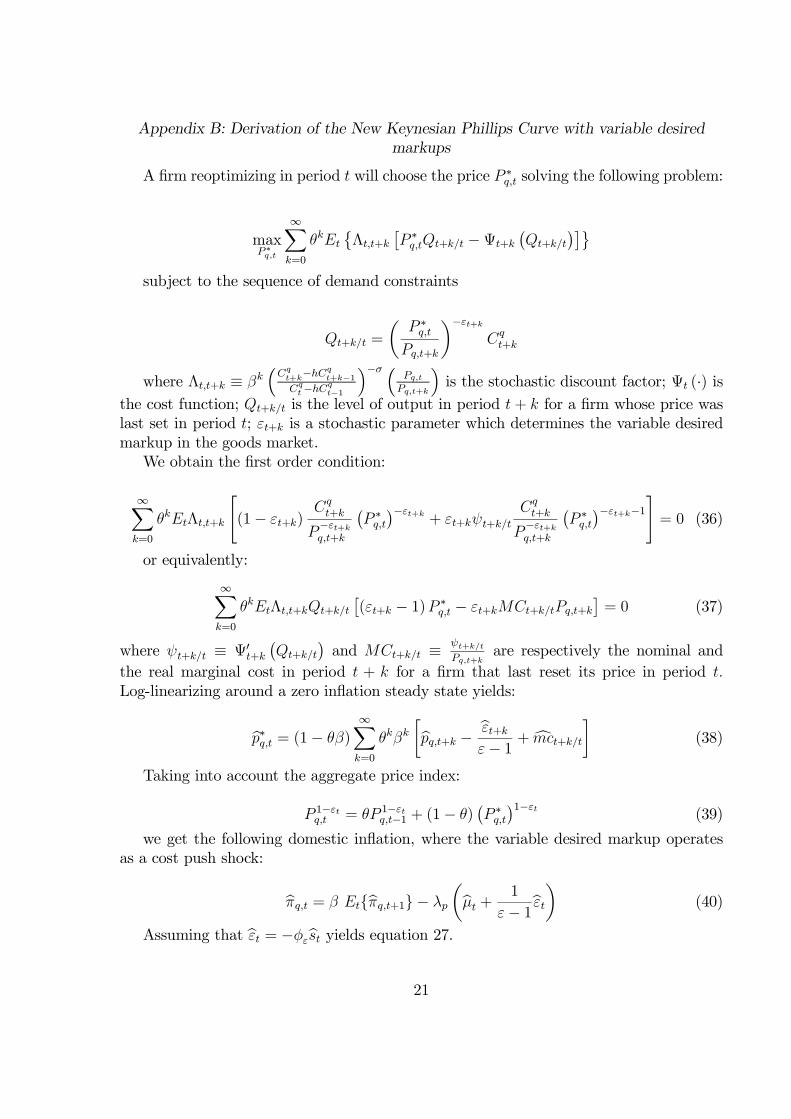
Appendix B: Derivation of the New Keynesian Phillips Curve with variable desired

markups

A firm reoptimizing in period t will choose the price P ∗

q,t solving the following problem:

maxP∗q,t

∞∑

k=0

θkEt

{Λt,t+k

[P ∗

q,tQt+k/t −Ψt+k(Qt+k/t

)]}

subject to the sequence of demand constraints

Qt+k/t =

(P ∗

q,t

Pq,t+k

)−εt+k

Cqt+k

where Λt,t+k ≡ βk(Cqt+k−hC

qt+k−1

Cqt−hCqt−1

)−σ (

Pq,tPq,t+k

)is the stochastic discount factor; Ψt (·) is

the cost function; Qt+k/t is the level of output in period t+ k for a firm whose price waslast set in period t; εt+k is a stochastic parameter which determines the variable desiredmarkup in the goods market.

We obtain the first order condition:

∞∑

k=0

θkEtΛt,t+k

[(1− εt+k)

Cqt+k

P−εt+kq,t+k

(P ∗

q,t

)−εt+k + εt+kψt+k/t

Cqt+k

P−εt+kq,t+k

(P ∗

q,t

)−εt+k−1

]= 0 (36)

or equivalently:

∞∑

k=0

θkEtΛt,t+kQt+k/t

[(εt+k − 1)P ∗

q,t − εt+kMCt+k/tPq,t+k]= 0 (37)

where ψt+k/t ≡ Ψ′t+k(Qt+k/t

)and MCt+k/t ≡

ψt+k/tPq,t+k

are respectively the nominal and

the real marginal cost in period t + k for a firm that last reset its price in period t.Log-linearizing around a zero inflation steady state yields:

p∗q,t = (1− θβ)∞∑

k=0

θkβk[pq,t+k −

εt+kε− 1

+ mct+k/t

](38)

Taking into account the aggregate price index:

P 1−εtq,t = θP 1−εt

q,t−1 + (1− θ)(P ∗

q,t

)1−εt (39)

we get the following domestic inflation, where the variable desired markup operatesas a cost push shock:

πq,t = β Et{πq,t+1} − λp

(µt +

1

ε− 1εt

)(40)

Assuming that εt = −φεst yields equation 27.

21

References

[1] Blanchard, Olivier J. and Jordi Gali (2007a), "The Macroeconomic Effects of OilShocks: Why are the 2000s So Different from the 1970s?" NBER Working Paper No.13368.

[2] Blanchard, Olivier J. and Jordi Gali (2007b), "Real Wage Rigidities and the NewKeynesian Model" Journal of Money, Credit and Banking vol. 39(s1), pages 35-65,02

[3] Blanchard, Olivier J. and Charles M. Kahn (1980), "The solution of Linear DifferenceModels under Rational Expectations," Econometrica, vol. 48(5), pages 1305-11.

[4] Boivin, Jean and Marc P. Giannoni (2002), "Assessing Changes in the MonetaryTransmission Mechanism: A VAR Approach," Economic Policy Review 8(1): 97-112.

[5] Boivin, Jean and Marc P. Giannoni (2006), "Has monetary policy become moreeffective?" The Review of Economics and Statistics, MIT Press, vol. 88(3), pages445-462.

[6] Calvo, Guillermo (1983), "Staggered Prices in a Utility Maximizing Framework,"Journal of Monetary Economics, 12, 383-398.

[7] Canova, Fabio and Luca Gambetti (2009), "Structural Changes in the US Economy:Is There a Role for Monetary Policy?", Journal of Economic Dynamics and Control33: 477-490.

[8] Canova, Fabio and Luca Gambetti (forthcoming), "Do Expectations matter? TheGreat Moderation Revisited", American Economic Journal: Macroeconomics.

[9] Castelnuovo, Efrem and Paolo Surico (forthcoming), "Monetary Policy, InflationExpectations and the Price Puzzle", Economic Journal.

[10] Christiano, Lawrence, Martin Eichenbaum and Charles Evans (2005), "NominalRigidities and the Dynamic Effects of a Shock to Monetary Policy", Journal of Po-litical Economy, 113, 1-45.

[11] Clarida, Richard, Jordi Gali and Mark Gertler (2000), "Monetary Policy Rules andMacroeconomic Stability: Evidence and Some Theory," Quarterly Journal of Eco-nomics 115(1): 147-80.

[12] Lubik, Thomas A. and Frank Schorfheide (2004), "Testing for Indeterminacy: Anapplication to US monetary Policy", American Economic Review, 94, 190-217.

[13] Rotemberg, Julio and Michael Woodford (1996), "Imperfect Competition and theEffects of Energy Price Increases on Economic Activity," Journal of Money, Creditand Banking, vol. 28, no. 4, 549-577.

22

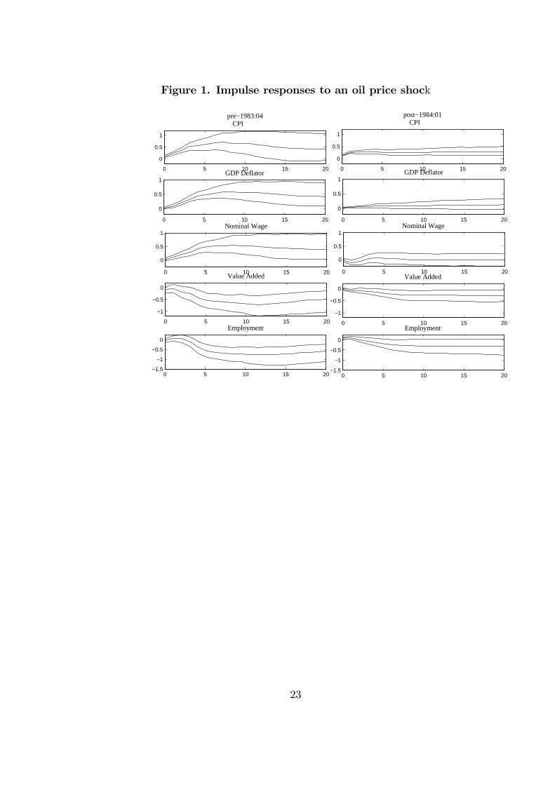
Figure 1. Impulse responses to an oil price shock

0 5 10 15 20

−1

−0.5

0

Value Added

0 5 10 15 20−1.5

−1

−0.5

0

Employment

0 5 10 15 20

0

0.5

1Nominal Wage

0 5 10 15 20

0

0.5

1GDP Deflator

0 5 10 15 20

0

0.5

1

pre−1983:04CPI

0 5 10 15 20

−1

−0.5

0

Value Added

0 5 10 15 20−1.5

−1

−0.5

0

Employment

0 5 10 15 20

0

0.5

1Nominal Wage

0 5 10 15 20

0

0.5

1GDP Deflator0 5 10 15 20

0

0.5

1

post−1984:01CPI

23

Figure 2. Domestic Inflation Expectations response to an oil price shock

0 2 4 6 8 10 12 14 16 18 20

0

0.02

0.04

0.06

0.08

0.1

0.12

–⊲– λ = 1–∗– λ = 0.4 Model Specification i–•– λ = 0.4 Model Specification ii

The remaining parameters are calibrated as follows: β=0.99, αn = 0.985, αm = 0.015,χ = 0.023, φ = 1, σ = 0.3, ǫ = 6, h = 0.9, γ = 0.9, θ = 0.7, φπ = 2.5.

24

Figure 3a. Estimated and Implied IRFs. Specification (i)

0 5 10 15 20−0.5

0

0.5

1

CPI

0 5 10 15 20−0.5

0

0.5

1

Pre−1983:04

0 5 10 15 20−0.5

0

0.5

1

GDP Deflator

0 5 10 15 20−0.5

0

0.5

1

Post−1984:01

0 5 10 15 20−0.5

0

0.5

1

Nominal Wage

0 5 10 15 20−0.5

0

0.5

1

0 5 10 15 20

−1

−0.5

0

Value Added

0 5 10 15 20

−1

−0.5

0

0 5 10 15 20

−1

−0.5

0

Employment

0 5 10 15 20

−1

−0.5

0

25

Figure 3b. Estimated and Implied IRFs. Specification (ii)

0 5 10 15 20

0

0.5

1

CPI

0 5 10 15 20

0

0.5

1

Post−1984:01

0 5 10 15 20

0

0.5

1

GDP Deflator

0 5 10 15 20

0

0.5

1

Pre−1983:04

0 5 10 15 20

0

0.5

1

Nominal Wage

0 5 10 15 20

0

0.5

1

0 5 10 15 20

−1

−0.5

0

Value Added

0 5 10 15 20

−1

−0.5

0

0 5 10 15 20

−1

−0.5

0

Employment

0 5 10 15 20

−1

−0.5

0

26

Figure 4. Impulse responses to an oil price shock. Level/Growthspecification of the VAR

0 5 10 15 20

−1

−0.5

0

Value Added

0 5 10 15 20

−1

−0.5

0

Employment

0 5 10 15 20

0

0.5

1Nominal Wage

0 5 10 15 20

0

0.5

1GDP Deflator

0 5 10 15 20

0

0.5

1

Pre−1983:04CPI

0 5 10 15 20−0.5

0

0.5Value Added

0 5 10 15 20−0.5

0

0.5Employment

0 5 10 15 20

0

0.5

1Nominal Wage

0 5 10 15 20

0

0.5

1GDP Deflator

0 5 10 15 20

0

0.5

1

Post−1984:01CPI

27

Figure 5a. Estimated and Implied IRFs. Level/growth VAR. Modelspecification (i)

0 5 10 15 20−0.5

0

0.5

1

CPI

0 5 10 15 20−0.5

0

0.5

1

Post−1984:01

0 5 10 15 20−0.5

0

0.5

1

GDP Deflator

0 5 10 15 20−0.5

0

0.5

1

Pre−1983:04

0 5 10 15 20−0.5

0

0.5

1

Nominal Wage

0 5 10 15 20−0.5

0

0.5

1

0 5 10 15 20−1

−0.5

0Value Added

0 5 10 15 20−1

−0.5

0

0 5 10 15 20−1

−0.5

0

Employment

0 5 10 15 20−1

−0.5

0

28

Figure 5b. Estimated and Implied IRFs. Level/growth VAR. Modelspecification (ii)

0 5 10 15 20−0.5

0

0.5

1

CPI

0 5 10 15 20−0.5

0

0.5

1

Post−1984:01

0 5 10 15 20−0.5

0

0.5

1

GDP Deflator

0 5 10 15 20−0.5

0

0.5

1

Pre−1983:04

0 5 10 15 20−0.5

0

0.5

1

Nominal Wage

0 5 10 15 20−0.5

0

0.5

1

0 5 10 15 20

−1

−0.5

0Value Added

0 5 10 15 20

−1

−0.5

0

0 5 10 15 20

−1

−0.5

0Employment

0 5 10 15 20

−1

−0.5

0

29

Figure 6a. Estimated and Implied IRFs. Leontief technology. Modelspecification (i)

0 5 10 15 20−0.5

0

0.5

1

Pre−1983:04

0 5 10 15 20−0.5

0

0.5

1

Post−1984:01

0 5 10 15 20−0.5

0

0.5

1

0 5 10 15 20−0.5

0

0.5

1

GDP Deflator

0 5 10 15 20−0.5

0

0.5

1

0 5 10 15 20−0.5

0

0.5

1

Nominal Wage

0 5 10 15 20

−1

−0.5

0

0 5 10 15 20

−1

−0.5

0

Value Added

0 5 10 15 20−1.5

−1

−0.5

0

CPI

0 5 10 15 20−1

−0.5

0Employment

30

Figure 6b. Estimated and Implied IRFs. Leontief technology. Modelspecification (ii)

0 5 10 15 20−0.5

0

0.5

1

pre−1983:04

0 5 10 15 20−0.5

0

0.5

1

post−1984:01

0 5 10 15 20−0.5

0

0.5

1

CPI

0 5 10 15 20−0.5

0

0.5

1

GDP Deflator

0 5 10 15 20−0.5

0

0.5

1

0 5 10 15 20−0.5

0

0.5

1

Nominal Wage

0 5 10 15 20

−1

−0.5

0

0 5 10 15 20

−1

−0.5

0

Value Added

0 5 10 15 20−1.5

−1

−0.5

0

0.5

0 5 10 15 20−1

−0.5

0

Employment

31