Why Are Saving Rates of Urban Households in - Eswar Prasad
38
93 American Economic Journal: Macroeconomics 2010, 2:1, 93–130 http://www.aeaweb.org/articles.php?doi=10.1257/mac.2.1.93 C hinese households save a lot, and their savings rates have increased in recent years. After remaining relatively flat during the early 1990s, the average sav- ings rate of urban households, relative to their disposable income, rose from 17 per- cent in 1995 to 24 percent in 2005. This increase took place against a background of rapid income growth and a real interest rate on bank deposits that has been low over this period ( and even negative in some years, as nominal deposit rates are capped by the government ) . In this paper, we attempt to understand the reasons behind this phenomenon of a rising household savings rate. To this end, we use data from the annual Urban Household Surveys conducted by China’s National Bureau of Statistics to analyze the evolution of the urban household savings rate over the period 1990–2005. We believe this is the first detailed examination of Chinese household savings behavior using micro data over a long span. 1 1 Most previous studies have relied on aggregate data ( e.g., Franco Modigliani and Shi Larry Cao 2004; Louis Kuijs 2006) or provincial-level data ( e.g., Yingyi Qian 1988; Aart Kraay 2000; Charles Yuji Horioka and Junmin Wan 2007). * Chamon: International Monetary Fund, Research Department, 700 19th Street, NW, Washington, DC 20431, (e-mail: [email protected]); Prasad: 440 Warren Hall, Department of Applied Economics and Management, Cornell University, Ithaca, NY 14853 (e-mail: [email protected]). We thank China’s National Bureau of Statistics and, in particular, Chen Xiaolong, Yu Qiumei, Wang Xiaoqing, and Cheng Xuebin for their collabora- tion on this project. This paper has benefited from comments by Chris Carroll, Angus Deaton, Karen Dynan, Charles Horioka, Marcelo Medeiros, Chang-Tai Hsieh, Nicholas Lardy, Junmin Wan, two anonymous referees, numerous International Monetary Fund (IMF) colleagues, and seminar participants at the IMF, the National Bureau of Economic Research China Workshop, the University of California at Berkeley, the NBER Summer Institute, Hong Kong University, and Hong Kong University of Science and Technology. The views expressed in this paper are those of the authors, and do not necessarily represent those of the IMF or IMF policy. † To comment on this article in the online discussion forum, or to view additional materials, visit the articles page at http://www.aeaweb.org/articles.php?doi=10.1257/mac.2.1.93. Why Are Saving Rates of Urban Households in China Rising? † By Marcos D. Chamon and Eswar S. Prasad* From 1995 to 2005, the average urban household savings rate in China rose by 7 percentage points, to about one-quarter of dispos- able income. Savings rates increased across all demographic groups, and the age profile of savings has an unusual pattern in recent years, with younger and older households having relatively high savings rates. We argue that these patterns are best explained by the rising private burden of expenditures on housing, education, and health care. These effects and precautionary motives may have been ampli- fied by financial underdevelopment, including constraints on bor- rowing against future income and low returns on financial assets. ( JEL D14, E21, O12, O18, P25, P36)
Transcript of Why Are Saving Rates of Urban Households in - Eswar Prasad
93
American Economic Journal: Macroeconomics 2010, 2:1, 93–130http://www.aeaweb.org/articles.php?doi=10.1257/mac.2.1.93
Chinese households save a lot, and their savings rates have increased in recent years. After remaining relatively flat during the early 1990s, the average sav-
ings rate of urban households, relative to their disposable income, rose from 17 per-cent in 1995 to 24 percent in 2005. This increase took place against a background of rapid income growth and a real interest rate on bank deposits that has been low over this period (and even negative in some years, as nominal deposit rates are capped by the government). In this paper, we attempt to understand the reasons behind this phenomenon of a rising household savings rate. To this end, we use data from the annual Urban Household Surveys conducted by China’s National Bureau of Statistics to analyze the evolution of the urban household savings rate over the period 1990–2005. We believe this is the first detailed examination of Chinese household savings behavior using micro data over a long span.1
1 Most previous studies have relied on aggregate data (e.g., Franco Modigliani and Shi Larry Cao 2004; Louis Kuijs 2006) or provincial-level data (e.g., Yingyi Qian 1988; Aart Kraay 2000; Charles Yuji Horioka and Junmin Wan 2007).
* Chamon: International Monetary Fund, Research Department, 700 19th Street, NW, Washington, DC 20431, (e-mail: [email protected]); Prasad: 440 Warren Hall, Department of Applied Economics and Management, Cornell University, Ithaca, NY 14853 (e-mail: [email protected]). We thank China’s National Bureau of Statistics and, in particular, Chen Xiaolong, Yu Qiumei, Wang Xiaoqing, and Cheng Xuebin for their collabora-tion on this project. This paper has benefited from comments by Chris Carroll, Angus Deaton, Karen Dynan, Charles Horioka, Marcelo Medeiros, Chang-Tai Hsieh, Nicholas Lardy, Junmin Wan, two anonymous referees, numerous International Monetary Fund (IMF) colleagues, and seminar participants at the IMF, the National Bureau of Economic Research China Workshop, the University of California at Berkeley, the NBER Summer Institute, Hong Kong University, and Hong Kong University of Science and Technology. The views expressed in this paper are those of the authors, and do not necessarily represent those of the IMF or IMF policy.
† To comment on this article in the online discussion forum, or to view additional materials, visit the articles page at http://www.aeaweb.org/articles.php?doi=10.1257/mac.2.1.93.
Why Are Saving Rates of Urban Households in China Rising? †
By Marcos D. Chamon and Eswar S. Prasad*
From 1995 to 2005, the average urban household savings rate in China rose by 7 percentage points, to about one-quarter of dispos-able income. Savings rates increased across all demographic groups, and the age profile of savings has an unusual pattern in recent years, with younger and older households having relatively high savings rates. We argue that these patterns are best explained by the rising private burden of expenditures on housing, education, and health care. These effects and precautionary motives may have been ampli-fied by financial underdevelopment, including constraints on bor-rowing against future income and low returns on financial assets. (JEL D14, E21, O12, O18, P25, P36)
Contents
Why Are Saving Rates of Urban Households in China Rising? † 93
I. Dataset 97
II. Stylized Facts 99
III. Demographic Effects on Household Savings Rates: A Decomposition Analysis 103
A. Estimation Strategy 104
B. Age, Cohort, and Time Effects in Household Savings Rates 105
IV. Potential Explanations 108
A. Habit Formation 108
B. Shifts in Social Expenditures 111
C. Durables Purchases and Savings 113
D. Housing Purchases and Savings 114
E. Effects of State Enterprise Restructuring on Saving Behavior 117
94 AMERICAN ECONOMIC JOURNAL: MACROECONOMICS JANUARY 2010
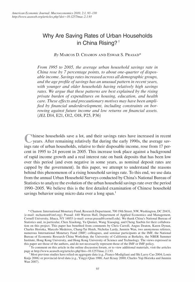
It is worth noting that the increase in household savings is not simply compen-sating for reduced savings by other sectors of the economy. Figure 1 shows that gross domestic savings in China has surged since 2000, climbing to over 50 percent of gross domestic product (GDP) in 2005. In particular, enterprise saving—includ-ing that of state-owned enterprises—has risen sharply in recent years. Government savings (which is subsequently used for public investment) has also increased. Household savings has declined as a percentage of national income even as it has increased as a share of household disposable income, but this is mainly because of a fall in the share of household income in national income.2 The aggregate (urban and rural) household savings rate has, in fact, risen by 6 percentage points over the last decade.
It is difficult to reconcile the phenomenon of a rising household savings rate with conventional intertemporal models of consumption. When trend income growth is high, households seeking to smooth their consumption should borrow against future income, especially if real interest rates are low. If that is not possible, households (particularly younger ones) should at least postpone their savings. But, as we show
2 In China, state-owned enterprises did not distribute profits to households or the government in the form of dividends. Beginning in 2008, the government began requiring modest dividend payments.
0
5
10
15
20
25
30
35
40
45
50
55
1992 1993 1994 1995 1996 1997 1998 1999 2000 2001 2002 2003 2004 2005
Year
Per
cent
age
Households
Enterprises
Government
Figure 1. Contributions to Gross Domestic Savings as a Percentage of GDP
Note: Household savings, shown here, are based on national accounts data, which imply higher savings rates than those based on household survey data (see Table A1).
Source: CEIC, National Bureau of Statistics (China), and International Monetary Fund (IMF).
VOL. 2 NO. 1 95CHAMON AND PRASAD: WHY ARE SAVING RATES IN CHINA RISING?
in this paper, savings rates have increased across all demographic groups, including those that can expect rapid income growth in the future.
We estimate how savings rates vary with time, age, and cohort (year of birth) of the household head, using a variant of the decomposition in Angus S. Deaton and Christina H. Paxson (1994). The most interesting result is that we find a U-shaped pattern of savings over the life cycle, wherein the younger and older households have the highest savings rates. This is the opposite of the traditional “hump-shaped” profile of savings over the life cycle in which young workers save very little (in anticipation of rising income), savings rates tend to peak when earnings potential is the highest (middle age), and then fall off as workers approach retirement. This relationship between age and savings rate differs considerably from the norm for other countries.
Demographic shifts do not go very far in explaining saving behavior. For instance, the cohorts most affected by the one-child policy are not among the highest savers. Even after we control for broader demographic shifts, there remains a substantial time trend in household savings rates, implying that the rising savings rates must be the result of economy-wide changes affecting all households. As with most other studies using household data, we also find very limited consumption smoothing over the life cycle.3
What can account for these patterns? Habit formation could drive up savings rates by restraining consumption growth despite high income growth (Christopher D. Carroll and David N. Weil 1994). However, we find little empirical support for that channel as consumption growth does not seem to have much persistence once we control for other factors. Instead, the declining public provision of education, health, and housing services (the breaking of the “iron rice bowl”) appears to have created new motives for saving. While health and education expenditures accounted for 2 percent of consumption expenditures among the households in our sample in 1995, this share rose to 14 percent by 2005.4 This can contribute to rising savings, as younger households accumulate assets to prepare for future education expenditures, and older households prepare for uncertain (and lumpy) health expenditures.
Moreover, there has been an extensive privatization of the housing stock. Only 17 percent of households in our sample owned their homes in 1990. By 2005, that figure had risen to 86 percent. Most house purchases were financed by the with-drawal of past savings, suggesting that this has been an important motive for house-hold savings over the past decade. Simple back-of-the-envelope calculations suggest that housing related motives could account for nearly a 3 percentage point increase in savings rates since the early 1990s. Many houses purchased under the housing reform process are of low quality, however, suggesting that as income levels rise and the capacity to buy better houses increases, savings rates could stay high on account
3 See, for example, Paxson (1996). Horioka and Wan (2007) use provincial-level data and also find a limited role for variables related to the age structure in explaining saving behavior. Modigliani and Shi Larry Cao (2004) find evidence in favor of the life-cycle hypothesis using aggregate (national level) data.
4 These expenditures are superior goods, with an income elasticity greater than one. Rapid income growth and the aging of the population have amplified the trend toward direct private expenditures on those services. The share of government (central and local) expenditures accounted for by expenditures on culture, education, science, and health care has fallen from 22 percent in 1995 to 18 percent in 2005.
96 AMERICAN ECONOMIC JOURNAL: MACROECONOMICS JANUARY 2010
of this motive, as the mortgage market is still underdeveloped. Indeed, given the durable nature of houses, households with good income growth prospects may con-tinue to have high savings in order to make down payments on higher quality houses commensurate with their future income.
The overall macroeconomic uncertainty associated with the transition to a market economy has contributed to precautionary savings motives, although we do not find strong evidence that the effect of macro uncertainty has been quantitatively impor-tant. One interesting result is that the cohorts that were in their 40s and 50s in 1990 tended to save more, perhaps because they are the ones most exposed to the uncer-tainties generated by the market-oriented reforms and do not have many working years ahead to benefit from those reforms.
We also investigate the target savings hypothesis, according to which households have a target level of savings. Since bank deposits are the primary financial assets for Chinese households, their savings rates are negatively correlated with real returns on bank deposits. We find some weak suggestive evidence that, even if taken at face value, points to a small effect. While cultural factors are often considered a promis-ing explanation for the high savings rates observed in East Asian economies, they cannot account for the trend in savings rates that is our primary focus in this paper.5
After examining the empirical relevance of various hypotheses individually, we estimate a composite regression to evaluate the relative importance of the most promising ones. We find that the risk of large health expenditures can explain high savings for households headed by older persons, and that savings are also higher for households whose composition portends large education expenditures in the future. These and other strands of evidence suggest that precautionary motives and the rising private burden of social expenditures has driven the increase in household savings rates. In the composite regression, the effects of home ownership status on savings are somewhat muted, on average, although we do find that owners of poor-quality homes (homes with values below the respective provincial median) have higher sav-ings rates than those with better homes. More interestingly, we find that owning a home is associated with sharply lower savings rates (4–7 percentage points) among young households, but not among older ones. The relatively high income levels of younger households also help explain their high savings rates. All of these effects are amplified in an environment of financial repression, which has resulted in the lack of instruments for borrowing against future income, limited opportunities for portfolio diversification, and low real returns on bank deposits.6 Of course, these channels can only account for an increase in the savings rate during an adjustment period. They cannot, by themselves, sustain high savings rates in the long run.
In the final section of this paper, we combine the empirical results with some macroeconomic data to discuss possible implications for the evolution of household savings in China. Our estimates suggest a modest role for projected demographic changes on household savings. Since our preferred explanations for the high and
5 Carroll, Byung-Kun Rhee, and Changyong Rhee (1994) compare the savings behavior of different immi-grant groups in Canada and find no evidence of cultural effects on savings.
6 A previous version of this paper has a simple model that highlights these points. The model builds on the work of Tullio Jappelli and Marco Pagano (1994), who illustrate how the interaction of rapid income growth and borrowing constraints due to financial underdevelopment can drive up savings rates.
VOL. 2 NO. 1 97CHAMON AND PRASAD: WHY ARE SAVING RATES IN CHINA RISING?
rising savings rates are related to China’s transition to a market economy and the underdeveloped financial system, it is possible that savings rates will decline as new financial instruments (for borrowing and for portfolio diversification) become preva-lent, and once households have accumulated a sufficiently large stock of assets to cope with the new economic environment. The shift from public to private provision of education, health, and housing can help explain rising savings rates during an adjustment period. Government policy toward social expenditures will be relevant for determining the longer term trajectory of savings based on this motive (Olivier J. Blanchard and Francesco Giavazzi 2006, emphasize this point). Thus, the insights obtained by moving from aggregate- to household-level data, and the analysis in this paper, can inform the debate on how to “rebalance” growth in China by stoking private consumption growth.
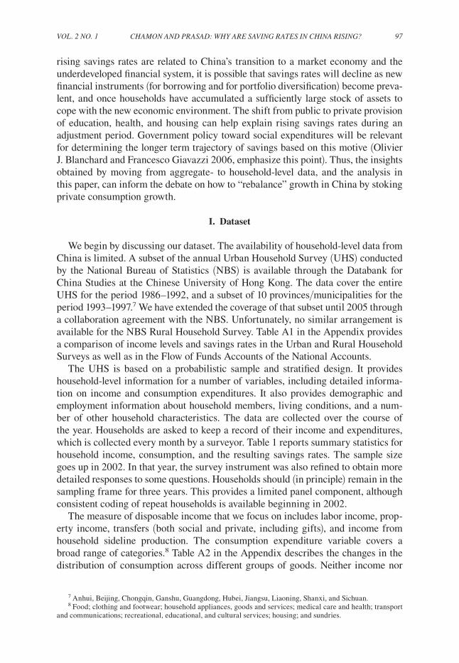
I. Dataset
We begin by discussing our dataset. The availability of household-level data from China is limited. A subset of the annual Urban Household Survey (UHS) conducted by the National Bureau of Statistics (NBS) is available through the Databank for China Studies at the Chinese University of Hong Kong. The data cover the entire UHS for the period 1986–1992, and a subset of 10 provinces/municipalities for the period 1993–1997.7 We have extended the coverage of that subset until 2005 through a collaboration agreement with the NBS. Unfortunately, no similar arrangement is available for the NBS Rural Household Survey. Table A1 in the Appendix provides a comparison of income levels and savings rates in the Urban and Rural Household Surveys as well as in the Flow of Funds Accounts of the National Accounts.
The UHS is based on a probabilistic sample and stratified design. It provides household-level information for a number of variables, including detailed informa-tion on income and consumption expenditures. It also provides demographic and employment information about household members, living conditions, and a num-ber of other household characteristics. The data are collected over the course of the year. Households are asked to keep a record of their income and expenditures, which is collected every month by a surveyor. Table 1 reports summary statistics for household income, consumption, and the resulting savings rates. The sample size goes up in 2002. In that year, the survey instrument was also refined to obtain more detailed responses to some questions. Households should (in principle) remain in the sampling frame for three years. This provides a limited panel component, although consistent coding of repeat households is available beginning in 2002.
The measure of disposable income that we focus on includes labor income, prop-erty income, transfers (both social and private, including gifts), and income from household sideline production. The consumption expenditure variable covers a broad range of categories.8 Table A2 in the Appendix describes the changes in the distribution of consumption across different groups of goods. Neither income nor
7 Anhui, Beijing, Chongqin, Ganshu, Guangdong, Hubei, Jiangsu, Liaoning, Shanxi, and Sichuan. 8 Food; clothing and footwear; household appliances, goods and services; medical care and health; transport
and communications; recreational, educational, and cultural services; housing; and sundries.
98 AMERICAN ECONOMIC JOURNAL: MACROECONOMICS JANUARY 2010
consumption measures capture the consumption value of owner-occupied housing.9 All flow variables are expressed on an annual basis and, where relevant, nominal vari-ables are deflated using the provincial consumer price index (CPI). We measure sav-ings as the difference between disposable income and consumption expenditures.10
A potential concern at this juncture is that the micro data indicate household savings rates lower than those suggested by the aggregate data taken from the Flow of Funds Accounts. The Flow of Funds data indicate a household savings rate of 32 percent in 2004, the last year for which those data are available. This is about 7 percentage points higher than the household survey-based estimate of the savings rate. The discrepancies between micro and macro data on savings ratios are an issue in virtually every country in which both types of data are available. Deaton (2005) documents systematic discrepancies whereby survey-based measures of income and consumption are different than those from the national accounts in most countries. Some of these differences can be traced to definitional issues.
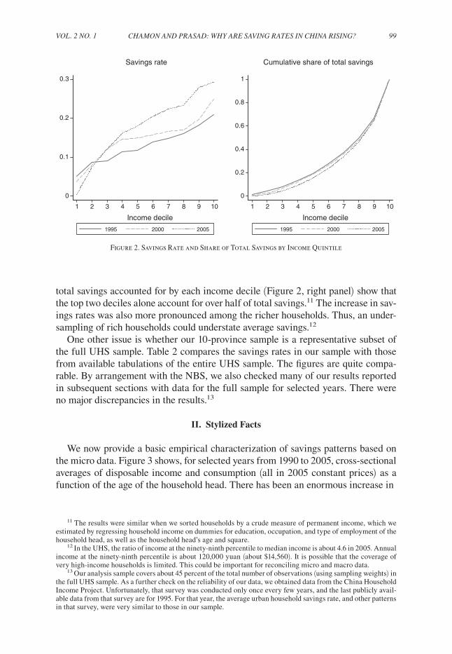
Perhaps, more importantly, it is usually difficult to get adequate survey response rates from high-income households. These households tend to have high savings propensities. Figure 2 (left panel) shows that savings rates are higher for the top deciles of the household income distribution covered in our sample. The shares of
9 Households report their estimate for the rental value of owner-occupied housing from 2002 onward. Later in the paper, we discuss how we separately estimate the rental value of owner-occupied houses for all years and incorporate it in the savings rate and income measures. These estimates are noisy, however, since it is rare for households to live in a rented private house. Hence, we use those estimates only in a few specifications to test the sensitivity of our main results.
10 This residual measure of savings includes transfer expenditures. This is appropriate to the extent that these expenditures reflect implicit risk sharing contracts among households. These transfer expenditures are fairly well spread across household demographic groups and different income levels. Our results are robust to their exclusion from savings (although the level of savings rates would decline).
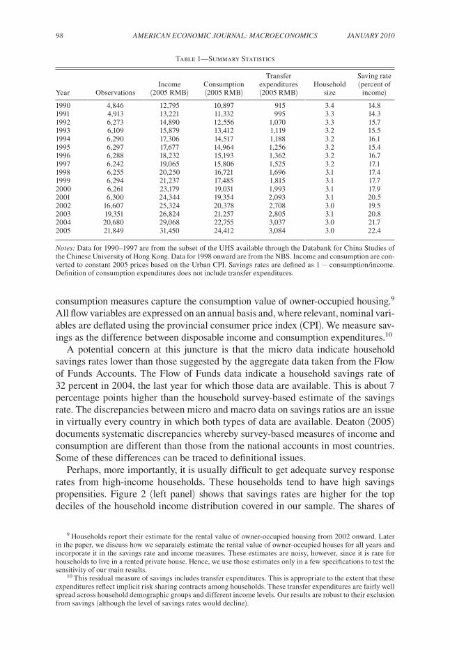
Table 1—Summary Statistics
Year ObservationsIncome
(2005 RMB)Consumption(2005 RMB)
Transfer expenditures(2005 RMB)
Householdsize
Saving rate(percent of
income)
1990 4,846 12,795 10,897 915 3.4 14.81991 4,913 13,221 11,332 995 3.3 14.31992 6,273 14,890 12,556 1,070 3.3 15.71993 6,109 15,879 13,412 1,119 3.2 15.51994 6,290 17,306 14,517 1,188 3.2 16.11995 6,297 17,677 14,964 1,256 3.2 15.41996 6,288 18,232 15,193 1,362 3.2 16.71997 6,242 19,065 15,806 1,525 3.2 17.11998 6,255 20,250 16,721 1,696 3.1 17.41999 6,294 21,237 17,485 1,815 3.1 17.72000 6,261 23,179 19,031 1,993 3.1 17.92001 6,300 24,344 19,354 2,093 3.1 20.52002 16,607 25,324 20,378 2,708 3.0 19.52003 19,351 26,824 21,257 2,805 3.1 20.82004 20,680 29,068 22,755 3,037 3.0 21.72005 21,849 31,450 24,412 3,084 3.0 22.4
Notes: Data for 1990–1997 are from the subset of the UHS available through the Databank for China Studies of the Chinese University of Hong Kong. Data for 1998 onward are from the NBS. Income and consumption are con-verted to constant 2005 prices based on the Urban CPI. Savings rates are defined as 1 − consumption/income. Definition of consumption expenditures does not include transfer expenditures.
VOL. 2 NO. 1 99CHAMON AND PRASAD: WHY ARE SAVING RATES IN CHINA RISING?
total savings accounted for by each income decile (Figure 2, right panel) show that the top two deciles alone account for over half of total savings.11 The increase in sav-ings rates was also more pronounced among the richer households. Thus, an under-sampling of rich households could understate average savings.12
One other issue is whether our 10-province sample is a representative subset of the full UHS sample. Table 2 compares the savings rates in our sample with those from available tabulations of the entire UHS sample. The figures are quite compa-rable. By arrangement with the NBS, we also checked many of our results reported in subsequent sections with data for the full sample for selected years. There were no major discrepancies in the results.13
II. Stylized Facts
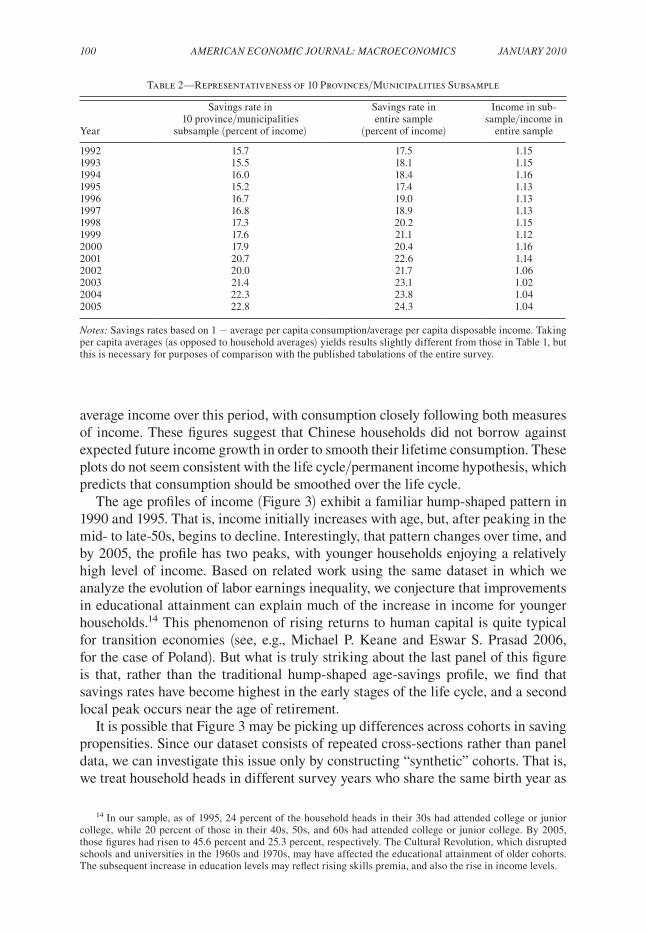
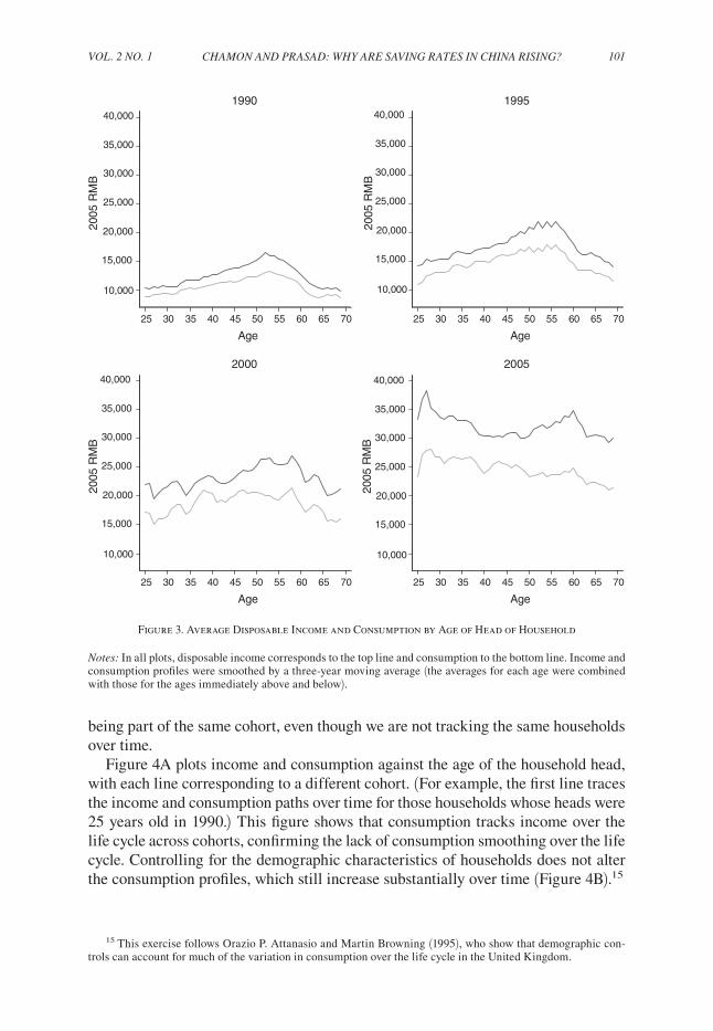
We now provide a basic empirical characterization of savings patterns based on the micro data. Figure 3 shows, for selected years from 1990 to 2005, cross-sectional averages of disposable income and consumption (all in 2005 constant prices) as a function of the age of the household head. There has been an enormous increase in
11 The results were similar when we sorted households by a crude measure of permanent income, which we estimated by regressing household income on dummies for education, occupation, and type of employment of the household head, as well as the household head’s age and square.
12 In the UHS, the ratio of income at the ninety-ninth percentile to median income is about 4.6 in 2005. Annual income at the ninety-ninth percentile is about 120,000 yuan (about $14,560). It is possible that the coverage of very high-income households is limited. This could be important for reconciling micro and macro data.
13 Our analysis sample covers about 45 percent of the total number of observations (using sampling weights) in the full UHS sample. As a further check on the reliability of our data, we obtained data from the China Household Income Project. Unfortunately, that survey was conducted only once every few years, and the last publicly avail-able data from that survey are for 1995. For that year, the average urban household savings rate, and other patterns in that survey, were very similar to those in our sample.
Savings rate Cumulative share of total savings
0
0.1
0.2
0.3
1 2 3 4 5 6 7 8 9 10
Income decile
1995 2000 2005
0
0.2
0.4
0.6
0.8
1
1 2 3 4 5 6 7 8 9 10
Income decile
1995 2000 2005
Figure 2. Savings Rate and Share of Total Savings by Income Quintile
100 AMERICAN ECONOMIC JOURNAL: MACROECONOMICS JANUARY 2010
average income over this period, with consumption closely following both measures of income. These figures suggest that Chinese households did not borrow against expected future income growth in order to smooth their lifetime consumption. These plots do not seem consistent with the life cycle/permanent income hypothesis, which predicts that consumption should be smoothed over the life cycle.
The age profiles of income (Figure 3) exhibit a familiar hump-shaped pattern in 1990 and 1995. That is, income initially increases with age, but, after peaking in the mid- to late-50s, begins to decline. Interestingly, that pattern changes over time, and by 2005, the profile has two peaks, with younger households enjoying a relatively high level of income. Based on related work using the same dataset in which we analyze the evolution of labor earnings inequality, we conjecture that improvements in educational attainment can explain much of the increase in income for younger households.14 This phenomenon of rising returns to human capital is quite typical for transition economies (see, e.g., Michael P. Keane and Eswar S. Prasad 2006, for the case of Poland). But what is truly striking about the last panel of this figure is that, rather than the traditional hump-shaped age-savings profile, we find that savings rates have become highest in the early stages of the life cycle, and a second local peak occurs near the age of retirement.
It is possible that Figure 3 may be picking up differences across cohorts in saving propensities. Since our dataset consists of repeated cross-sections rather than panel data, we can investigate this issue only by constructing “synthetic” cohorts. That is, we treat household heads in different survey years who share the same birth year as
14 In our sample, as of 1995, 24 percent of the household heads in their 30s had attended college or junior college, while 20 percent of those in their 40s, 50s, and 60s had attended college or junior college. By 2005, those figures had risen to 45.6 percent and 25.3 percent, respectively. The Cultural Revolution, which disrupted schools and universities in the 1960s and 1970s, may have affected the educational attainment of older cohorts. The subsequent increase in education levels may reflect rising skills premia, and also the rise in income levels.
Table 2—Representativeness of 10 Provinces/Municipalities Subsample
Year
Savings rate in10 province/municipalities
subsample (percent of income)
Savings rate in entire sample
(percent of income)
Income in sub-sample/income in
entire sample
1992 15.7 17.5 1.151993 15.5 18.1 1.151994 16.0 18.4 1.161995 15.2 17.4 1.131996 16.7 19.0 1.131997 16.8 18.9 1.131998 17.3 20.2 1.151999 17.6 21.1 1.122000 17.9 20.4 1.162001 20.7 22.6 1.142002 20.0 21.7 1.062003 21.4 23.1 1.022004 22.3 23.8 1.042005 22.8 24.3 1.04
Notes: Savings rates based on 1 − average per capita consumption/average per capita disposable income. Taking per capita averages (as opposed to household averages) yields results slightly different from those in Table 1, but this is necessary for purposes of comparison with the published tabulations of the entire survey.
VOL. 2 NO. 1 101CHAMON AND PRASAD: WHY ARE SAVING RATES IN CHINA RISING?
being part of the same cohort, even though we are not tracking the same households over time.
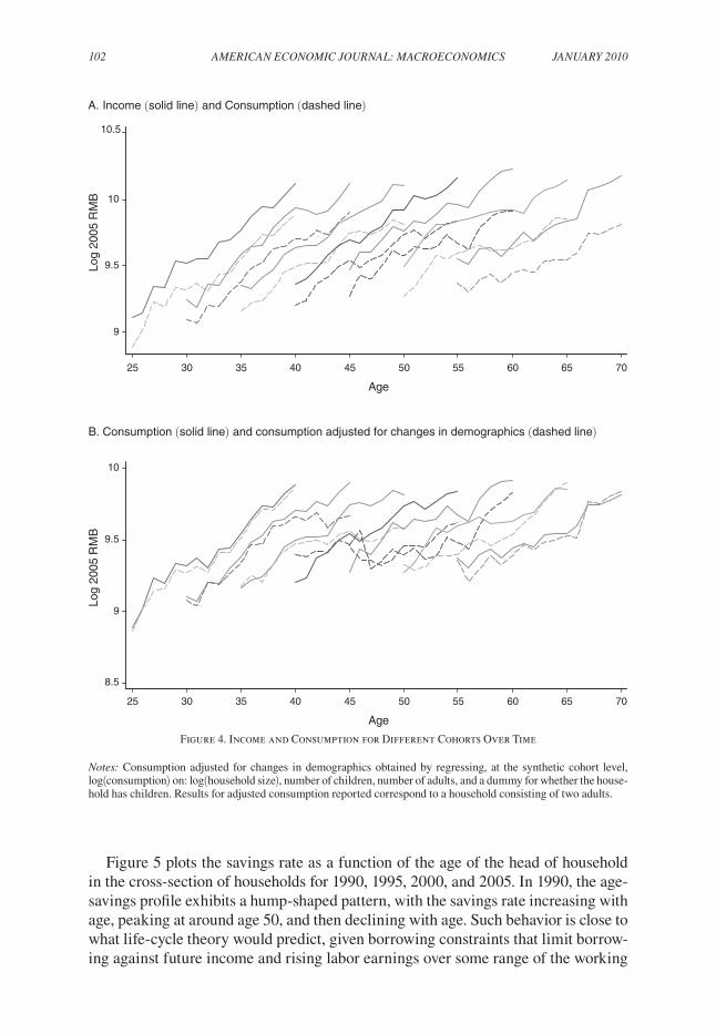
Figure 4A plots income and consumption against the age of the household head, with each line corresponding to a different cohort. (For example, the first line traces the income and consumption paths over time for those households whose heads were 25 years old in 1990.) This figure shows that consumption tracks income over the life cycle across cohorts, confirming the lack of consumption smoothing over the life cycle. Controlling for the demographic characteristics of households does not alter the consumption profiles, which still increase substantially over time (Figure 4B).15
15 This exercise follows Orazio P. Attanasio and Martin Browning (1995), who show that demographic con-trols can account for much of the variation in consumption over the life cycle in the United Kingdom.
10,000
15,000
20,000
25,000
30,000
35,000
40,000
2005
RM
B
25 30 35 40 45 50 55 60 65 70
Age
1990
2005
RM
B
25 30 35 40 45 50 55 60 65 70
Age
199520
05 R
MB
25 30 35 40 45 50 55 60 65 70
Age
200020
05 R
MB
25 30 35 40 45 50 55 60 65 70
Age
2005
10,000
15,000
20,000
25,000
30,000
35,000
40,000
10,000
15,000
20,000
25,000
30,000
35,000
40,000
10,000
15,000
20,000
25,000
30,000
35,000
40,000
Figure 3. Average Disposable Income and Consumption by Age of Head of Household
Notes: In all plots, disposable income corresponds to the top line and consumption to the bottom line. Income and consumption profiles were smoothed by a three-year moving average (the averages for each age were combined with those for the ages immediately above and below).
102 AMERICAN ECONOMIC JOURNAL: MACROECONOMICS JANUARY 2010
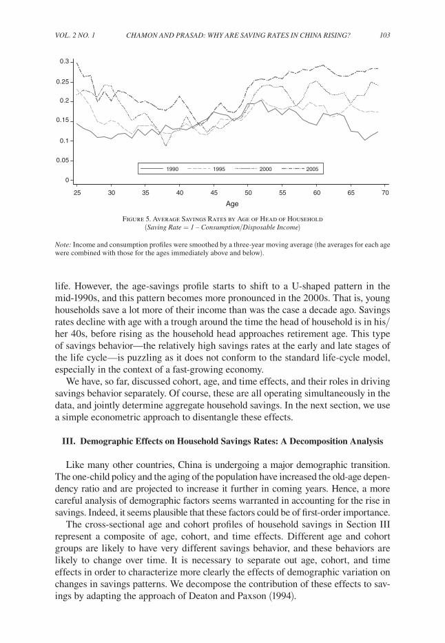
Figure 5 plots the savings rate as a function of the age of the head of household in the cross-section of households for 1990, 1995, 2000, and 2005. In 1990, the age-savings profile exhibits a hump-shaped pattern, with the savings rate increasing with age, peaking at around age 50, and then declining with age. Such behavior is close to what life-cycle theory would predict, given borrowing constraints that limit borrow-ing against future income and rising labor earnings over some range of the working
A. Income (solid line) and Consumption (dashed line)
9
9.5
10
10.5
Log
2005
RM
B
25 30 35 40 45 50 55 60 65 70
Age
B. Consumption (solid line) and consumption adjusted for changes in demographics (dashed line)
8.5
9
9.5
10
Log
2005
RM
B
25 30 35 40 45 50 55 60 65 70
Age
Figure 4. Income and Consumption for Different Cohorts Over Time
Notes: Consumption adjusted for changes in demographics obtained by regressing, at the synthetic cohort level, log(consumption) on: log(household size), number of children, number of adults, and a dummy for whether the house-hold has children. Results for adjusted consumption reported correspond to a household consisting of two adults.
VOL. 2 NO. 1 103CHAMON AND PRASAD: WHY ARE SAVING RATES IN CHINA RISING?
life. However, the age-savings profile starts to shift to a U-shaped pattern in the mid-1990s, and this pattern becomes more pronounced in the 2000s. That is, young households save a lot more of their income than was the case a decade ago. Savings rates decline with age with a trough around the time the head of household is in his/her 40s, before rising as the household head approaches retirement age. This type of savings behavior—the relatively high savings rates at the early and late stages of the life cycle—is puzzling as it does not conform to the standard life-cycle model, especially in the context of a fast-growing economy.
We have, so far, discussed cohort, age, and time effects, and their roles in driving savings behavior separately. Of course, these are all operating simultaneously in the data, and jointly determine aggregate household savings. In the next section, we use a simple econometric approach to disentangle these effects.
III. Demographic Effects on Household Savings Rates: A Decomposition Analysis
Like many other countries, China is undergoing a major demographic transition. The one-child policy and the aging of the population have increased the old-age depen-dency ratio and are projected to increase it further in coming years. Hence, a more careful analysis of demographic factors seems warranted in accounting for the rise in savings. Indeed, it seems plausible that these factors could be of first-order importance.
The cross-sectional age and cohort profiles of household savings in Section III represent a composite of age, cohort, and time effects. Different age and cohort groups are likely to have very different savings behavior, and these behaviors are likely to change over time. It is necessary to separate out age, cohort, and time effects in order to characterize more clearly the effects of demographic variation on changes in savings patterns. We decompose the contribution of these effects to sav-ings by adapting the approach of Deaton and Paxson (1994).
0
0.05
0.1
0.15
0.2
0.25
0.3
25 30 35 40 45 50 55 60 65 70
Age
1990 1995 2000 2005
Figure 5. Average Savings Rates by Age of Head of Household (Saving Rate = 1 – Consumption/Disposable Income)
Note: Income and consumption profiles were smoothed by a three-year moving average (the averages for each age were combined with those for the ages immediately above and below).
104 AMERICAN ECONOMIC JOURNAL: MACROECONOMICS JANUARY 2010
A. Estimation Strategy
If there are no shocks to income, and the real interest rate is constant, then the life-cycle hypothesis predicts that consumption at any given age should be propor-tional to lifetime resources, with the constant of proportionality depending on the age of the household head and the real interest rate. That is,
cha = fh(a)Wh,
where cha denotes the consumption of household h headed by an individual of age a and with lifetime resources Wh . Taking logs of the expression above and averaging it based on age and year of birth b yields
____
ln cab = _____
ln f (a) + ____
ln Wb .
In our estimation, the age effects _____
ln f (a) are captured by a vector of age dummies, and the lifetime resources
____ ln Wb are characterized by a vector of cohort (year of
birth) and time dummies. The estimated consumption equation is
(1) ____
ln cab = D aαc + D bγc + D tθc + εc,
where Da, Db, and Dt are matrices of age, year of birth, and year dummies; αc, γc, and θc are the corresponding age, cohort, and year effects on consumption; and εc is the error term. The year fixed effects should capture differences in consump-tion resulting from aggregate shocks and from China’s steady income growth. Each observation in this regression is weighted by the square root of the number of origi-nal observations that its average is based on.
Since age minus cohort equals year plus a constant, in the absence of constraints on these dummies, any trend could be the result of different combinations of year, age, and cohort effects. Deaton and Paxson (1994) identify age and cohort effects by imposing the constraint that the year effects must add up to zero and be orthogo-nal to a time trend. This constraint forces the decomposition to attribute the rising income and consumption over time to age and cohort effects (e.g., younger cohorts being much richer than older ones and, for a given cohort, income and consumption rising rapidly with age), overwhelming most of the other variation in consumption and savings behavior. Our objective is to disentangle differences in savings behavior across age and cohort groups, controlling for the rising economy-wide income level. Hence, rather than constraining the year effects, we restrict the cohort effects to add up to zero and be orthogonal to a trend.16,17 That is, we impose the constraints
16 We are grateful to Deaton for this suggestion.17 The life cycle hypothesis predicts how consumption should vary with age, but does not have implications
for how it should vary with the year of birth (after controlling for age and rising incomes over time). Hence, our identifying restriction doesn’t prevent us from testing that hypothesis.
VOL. 2 NO. 1 105CHAMON AND PRASAD: WHY ARE SAVING RATES IN CHINA RISING?
∑ b
γ c = 0, and ∑ b
γ c b = 0.
If the age profile of income is invariant to economic growth (i.e., if economic growth raises the lifetime resources of younger cohorts but does not alter the man-ner in which income is distributed over their life cycle), then income can also be expressed as a function of age and lifetime resources.18 We estimate an equation for disposable income that is analogous to the one for consumption:
(2) ____
ln yab = D aα y + D bγ y + D tθy + εy,
where α y, γy, and θy correspond to the age, cohort, and year effects on income; and εy is the error term. Once we have estimated the effects of a variable on consumption and income, we can compute its resulting effect on the household savings rate. When estimating these equations, we also include the following demographic controls: log (family size) and the share of individuals in the household aged 0–4, 5–9, 10–14, 15–19, and 20 or above.19
B. Age, Cohort, and Time Effects in Household Savings Rates
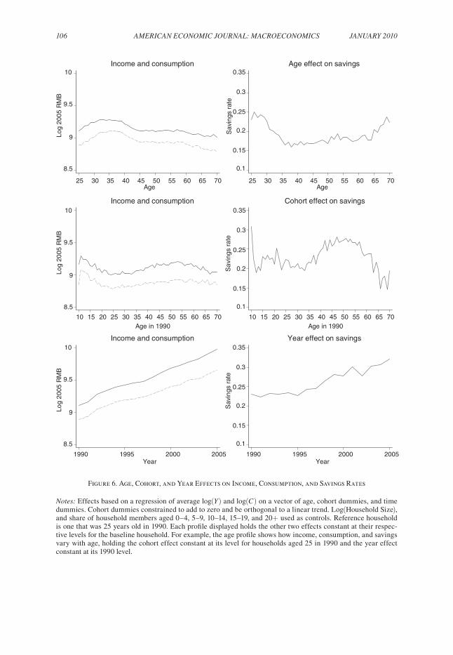
Figure 6 shows the estimated age and cohort profiles of income, consumption, and savings rates. The profile for one type of effect assumes that the others are kept constant. We take as our baseline household one in which the head of house-hold was 25 years old in 1990. For example, the age profile shows how income and consumption would vary with age holding the cohort effect constant at the level for the cohort born in 1965 and the year effect at its 1990 level (as if it was possible to change the age while holding the year and year of birth constant). Similarly, the cohort profile shows how income and consumption would vary with year of birth holding constant the age effect at its level for 25-year-olds and the year effect at its 1990 level. Finally, the year profile shows the variation over time holding constant the age effect at its level for 25-year-olds and the cohort effect at the level of those born in 1965.
The results confirm that consumption (dashed line) tends to track income (solid line). The age effects show that income and consumption initially increase with age before steadily declining. The implied effect on the savings rate, approximated as log (Y) − log (C), is similar to the savings rate profile as a function of age observed in the cross-section for the recent years (although the amplitude of the movements
18 While this may seem at odds with the descriptive plots presented above, the latter combine age with cohort and time effects, and are not directly comparable. This separability assumption provides a rough approximation for the decomposition of income in a parsimonious manner.
19 Later in the paper, we also control for the share of household members aged 60 or above. We omit that control here, as it is correlated with the age of the head of household, one of the main variables of interest in this section. We assume that a household headed by an individual with age a will have income and consumption pat-terns similar to those of an individual of age a. In an earlier version of this paper, we showed that the two variables are closely related in our data, except at the tails of the age distribution.
106 AMERICAN ECONOMIC JOURNAL: MACROECONOMICS JANUARY 2010
8.5
9
9.5
10
Log
2005
RM
B
25 30 35 40 45 50 55 60 65 70Age
Income and consumption
0.1
0.15
0.2
0.25
0.3
0.35
Sav
ings
rat
e
25 30 35 40 45 50 55 60 65 70Age
Age effect on savingsLo
g 20
05 R
MB
10 15 20 25 30 35 40 45 50 55 60 65 70Age in 1990
Income and consumption
Sav
ings
rat
e
10 15 20 25 30 35 40 45 50 55 60 65 70Age in 1990
Cohort effect on savings
Log
2005
RM
B
1990 1995 2000 2005Year
Income and consumption
Sav
ings
rat
e
1990 1995 2000 2005Year
Year effect on savings
8.5
9
9.5
10
0.1
0.15
0.2
0.25
0.3
0.35
8.5
9
9.5
10
0.1
0.15
0.2
0.25
0.3
0.35
Figure 6. Age, Cohort, and Year Effects on Income, Consumption, and Savings Rates
Notes: Effects based on a regression of average log(Y) and log(C) on a vector of age, cohort dummies, and time dummies. Cohort dummies constrained to add to zero and be orthogonal to a linear trend. Log(Household Size), and share of household members aged 0–4, 5–9, 10–14, 15–19, and 20+ used as controls. Reference household is one that was 25 years old in 1990. Each profile displayed holds the other two effects constant at their respec-tive levels for the baseline household. For example, the age profile shows how income, consumption, and savings vary with age, holding the cohort effect constant at its level for households aged 25 in 1990 and the year effect constant at its 1990 level.
VOL. 2 NO. 1 107CHAMON AND PRASAD: WHY ARE SAVING RATES IN CHINA RISING?
is smaller).20 It indicates that young households save substantially, but then savings rates gradually decline (by about 10 percentage points), reaching a trough around age 45. Savings rates increase rapidly after the age of the household head crosses the mid-40s, and remain high even among much older households.21 The increase from age 45 to age 65 is about 6 percentage points. This U-shaped pattern of savings is highly unusual, and it is a striking departure from the traditional hump-shaped pattern found in most other economies. It is also inconsistent with the life-cycle/permanent income hypothesis.22
The cohort profiles of income, consumption, and savings suggest that younger and older cohorts had relatively higher income than those that were in their 20s and 30s in 1990. The resulting effect on savings suggests that the higher saving cohorts are those that were in their 40s and 50s in 1990 (saving about 7.5 percentage points more than later cohorts). This is an interesting result, and may be capturing the fact that those cohorts may have been particularly hard hit by the reform process and bore the brunt of the increase in uncertainty associated with the move toward a mar-ket economy. The sharp increase in the savings rate in the later working years is also consistent with postponing retirement savings until retirement is near, which is the optimal response to rapid expected income growth.
It is worth noting that cohorts that were in their 30s in 1990, arguably the ones most affected by the one-child policy adopted in the late 1970s, are not high-saving cohorts. In fact, their average cohort effect on savings is close to the average for all cohorts. This is not to say that the one-child policy had no effect on savings, but, simply, that we cannot find a distinct effect on different cohorts based on the time of introduction of the policy.23
Finally, we turn to the time profile. As expected, the (unrestricted) time effects point to upward trends in income and consumption. Income grows more rapidly than consumption, resulting in a strong increasing trend in savings. The time effects explain a 9 percentage point increase in the savings rate from 1990 to 2005. This is a large figure, particularly considering the host of life-cycle and demographic charac-teristics we are controlling for. This suggests a limited role for demographic changes in explaining the rise in Chinese household savings over the last decade and a half. The results were similar when we dropped the controls for family composition or dropped cohort effects.
20 This approximation allows us to linearly separate the different effects in the estimated regressions. It yields savings rates slightly higher than we would get using 1 − C/Y.
21 Pierre-Olivier Gourinchas and Jonathan A. Parker (2002) estimate that young US households behave as buffer-stock savers, and they start to save for retirement when the household head is around age 40. David J. McKenzie (2006) finds that precautionary behavior in the face of rising income uncertainty may have reduced the incentives for younger cohorts in Taiwan Province of China to borrow in anticipation of rising lifetime incomes.
22 We reiterate that this pattern cannot be explained simply by rising income and consumption over time, since our decomposition already allows for that (through the unrestricted time effects).
23 The one-child policy could still have affected other cohorts. For example, younger cohorts will not be able to share the burden of supporting elderly parents with siblings. On the other hand, rapid income growth would increase the ability of that single child to support the parents.
108 AMERICAN ECONOMIC JOURNAL: MACROECONOMICS JANUARY 2010
IV. Potential Explanations
Since demographic shifts related to changes in the relative sizes of cohorts do not seem to be able to account for the increase in household savings, we now dis-cuss a variety of alternative hypotheses that could account for the deviations from the predictions of the traditional life-cycle/permanent income hypothesis. We also present some data and preliminary evidence of the quantitative relevance of these hypotheses in explaining the patterns we have documented. We first investigate these hypotheses individually in order to ascertain their empirical relevance before turn-ing (in Section VI) to a framework that allows us to assess their relative importance.
A. Habit Formation
Habit formation implies that consumption reacts slowly to rising income. This could explain why savings rates may increase during a period of rapid income growth. This hypothesis has been used to explain why rapidly growing countries have high savings rates (Carroll and Weil 1994), but the evidence in favor of it is weaker in household data (see, e.g., Karen E. Dynan 2000; Wooheon Rhee 2004).
Ideally, one would like to have panel data to test this hypothesis. The UHS rotates one-third of surveyed households out of the sample every year, implying that most households are in the survey for three years. This gives us a limited panel compo-nent to study household consumption behavior. The identification codes for track-ing households over time are, however, kept consistent only from 2002. Prior to that year, household identifier codes were often reset or assigned to replacement households when original households dropped out of the survey. Hence, we have to match households based on other characteristics as well. We make very conservative assumptions to ensure that we are picking up the same households over time, yield-ing a far smaller sample before 2002.24
Habit formation implies that current consumption growth is positively correlated with past consumption growth. Following Dynan (2000), we estimate the following equation:
Δlog (ci,t) = α + βΔlog (ci,t−1) + γi θi,t + εi,t ,
where ∆log (ci,t) is the log-change in nondurables consumption for household i and θi,t is a vector of household characteristics.25 We estimate this regression using the panel of households in our sample, as well as different pseudo-panels. We restrict the sample to households in which the head is 25–69 years old, and exclude those in which the head is a student, has lost the ability to work, is unemployed, or is waiting for an assignment. Table 3 presents the estimates for the coefficient on
24 In addition to using the household identifier codes, we ensure matching of household composition and characteristics of the household head and spouse (if present) by age (shifted by one year), education level, and type of employment.
25 Nondurables consumption is defined as total consumption minus expenditures on durables related to house-hold appliances, transportation, and educational and recreational goods.
VOL. 2 NO. 1 109CHAMON AND PRASAD: WHY ARE SAVING RATES IN CHINA RISING?
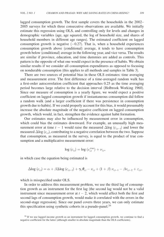
lagged consumption growth. The first sample covers the households in the 2002–2005 surveys for which three consecutive observations are available. We initially estimate this regression using OLS, and controlling only for levels and changes in demographic variables (age, age squared, the log of household size, and shares of household members in different age ranges). The estimated coefficient on lagged consumption growth is negative (−0.27). That is, when a household experiences consumption growth above (conditional) average, it tends to have consumption growth below (conditional) average in the following year, and vice versa. The results are similar if province, education, and time dummies are added as controls. This pattern is the opposite of what one would expect in the presence of habits. We obtain similar results if we consider all consumption expenditures as opposed to focusing on nondurable consumption (this applies to all methods and samples in Table 3).
There are two sources of potential bias in these OLS estimates: time averaging and measurement error. The first difference of a time-averaged random walk has a first-order autocorrelation coefficient that approaches 0.25 as the time averaging period becomes large relative to the decision interval (Holbrook Working 1960). Since our measure of consumption is a yearly figure, we would expect a positive coefficient on lagged consumption growth if instantaneous consumption did follow a random walk (and a larger coefficient if there was persistence in consumption growth due to habits). If we could properly account for this bias, it would presumably increase the absolute magnitude of the negative coefficient on lagged consumption growth, which would, in fact, strengthen the evidence against habit formation.
Our estimates may also be influenced by measurement error in consumption, which could bias the estimates downward. For example, an unusually high mea-surement error at time t − 1 would raise the measured ∆log (ci,t−1) and lower the measured ∆log (ci,t), contributing to a negative correlation between the two. Suppose that consumption, as measured in the survey, is equal to the product of true con-sumption and a multiplicative measurement error:
log (ci,t) = log ( c i,t true ) + νi,t ,
in which case the equation being estimated is
∆log (ci,t) = α + βΔlog (ci,t−1) + γ i θi,t − νi,t + (1 + β) νi,t−1 − βνi,t−2 + εi,t ,
which is misspecified under OLS.In order to address this measurement problem, we use the third lag of consump-
tion growth as an instrument for the first lag (the second lag would not be a valid instrument since measurement error at t − 2, which would affect both the first and second lags of consumption growth, would make it correlated with the errors in the second-stage regression). Since our panel covers three years, we can only estimate this specification using synthetic cohorts in a pseudo-panel.26
26 If we use lagged income growth as an instrument for lagged consumption growth, we continue to find a negative coefficient for the latter (although smaller in absolute magnitude than the OLS coefficients).
110 AMERICAN ECONOMIC JOURNAL: MACROECONOMICS JANUARY 2010
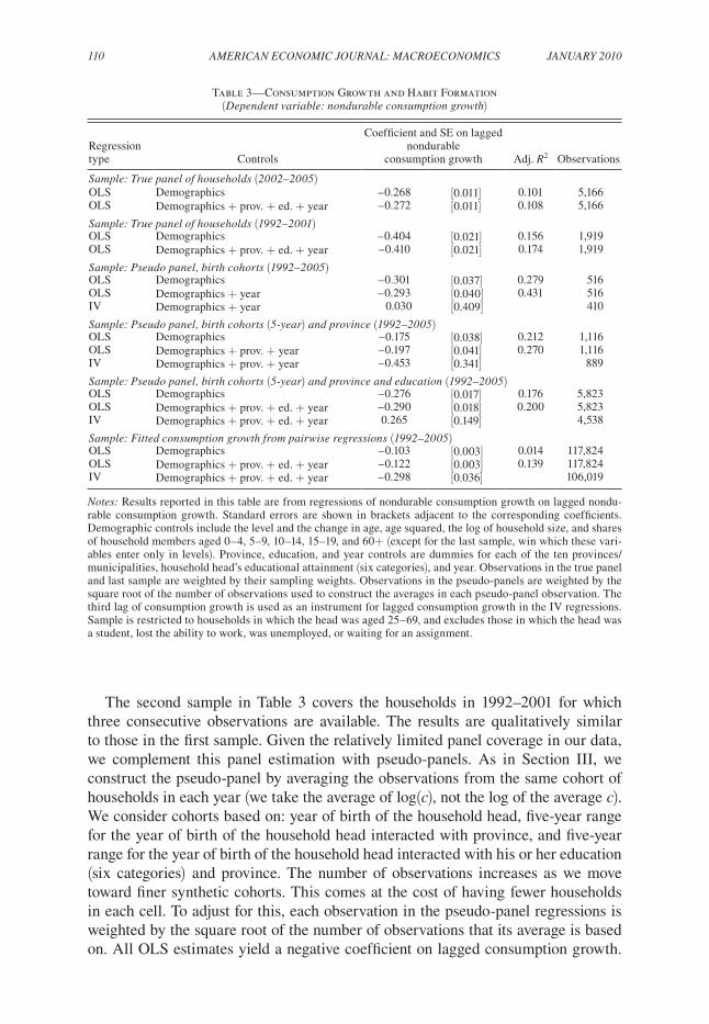
The second sample in Table 3 covers the households in 1992–2001 for which three consecutive observations are available. The results are qualitatively similar to those in the first sample. Given the relatively limited panel coverage in our data, we complement this panel estimation with pseudo-panels. As in Section III, we construct the pseudo-panel by averaging the observations from the same cohort of households in each year (we take the average of log(c), not the log of the average c). We consider cohorts based on: year of birth of the household head, five-year range for the year of birth of the household head interacted with province, and five-year range for the year of birth of the household head interacted with his or her education (six categories) and province. The number of observations increases as we move toward finer synthetic cohorts. This comes at the cost of having fewer households in each cell. To adjust for this, each observation in the pseudo-panel regressions is weighted by the square root of the number of observations that its average is based on. All OLS estimates yield a negative coefficient on lagged consumption growth.
Table 3—Consumption Growth and Habit Formation (Dependent variable: nondurable consumption growth)
Regression type Controls
Coefficient and SE on lagged nondurable
consumption growth Adj. R2 Observations
Sample: True panel of households (2002–2005)OLS Demographics –0.268 [0.011] 0.101 5,166OLS Demographics + prov. + ed. + year –0.272 [0.011] 0.108 5,166
Sample: True panel of households (1992–2001)OLS Demographics –0.404 [0.021] 0.156 1,919OLS Demographics + prov. + ed. + year –0.410 [0.021] 0.174 1,919
Sample: Pseudo panel, birth cohorts (1992–2005)OLS Demographics –0.301 [0.037] 0.279 516OLS Demographics + year –0.293 [0.040] 0.431 516IV Demographics + year 0.030 [0.409] 410
Sample: Pseudo panel, birth cohorts (5-year) and province (1992–2005)OLS Demographics –0.175 [0.038] 0.212 1,116OLS Demographics + prov. + year –0.197 [0.041] 0.270 1,116IV Demographics + prov. + year –0.453 [0.341] 889
Sample: Pseudo panel, birth cohorts (5-year) and province and education (1992–2005)OLS Demographics –0.276 [0.017] 0.176 5,823OLS Demographics + prov. + ed. + year –0.290 [0.018] 0.200 5,823IV Demographics + prov. + ed. + year 0.265 [0.149] 4,538
Sample: Fitted consumption growth from pairwise regressions (1992–2005)OLS Demographics –0.103 [0.003] 0.014 117,824OLS Demographics + prov. + ed. + year –0.122 [0.003] 0.139 117,824IV Demographics + prov. + ed. + year –0.298 [0.036] 106,019
Notes: Results reported in this table are from regressions of nondurable consumption growth on lagged nondu-rable consumption growth. Standard errors are shown in brackets adjacent to the corresponding coefficients. Demographic controls include the level and the change in age, age squared, the log of household size, and shares of household members aged 0–4, 5–9, 10–14, 15–19, and 60+ (except for the last sample, win which these vari-ables enter only in levels). Province, education, and year controls are dummies for each of the ten provinces/municipalities, household head’s educational attainment (six categories), and year. Observations in the true panel and last sample are weighted by their sampling weights. Observations in the pseudo-panels are weighted by the square root of the number of observations used to construct the averages in each pseudo-panel observation. The third lag of consumption growth is used as an instrument for lagged consumption growth in the IV regressions. Sample is restricted to households in which the head was aged 25–69, and excludes those in which the head was a student, lost the ability to work, was unemployed, or waiting for an assignment.
VOL. 2 NO. 1 111CHAMON AND PRASAD: WHY ARE SAVING RATES IN CHINA RISING?
Some of the IV estimates yield positive coefficients, but they are not statistically significant.27 This may be partly driven by the fact that the instrument used is very weak in the first stage (its coefficient is not significant at the 5 percent level in any of the regressions, and is only significant at the 10 percent level for the finest of the three cohort definitions). While the use of synthetic cohorts can reduce the measure-ment error due to idiosyncrasies in the way households record their expenditures, it creates an additional measurement problem stemming from the fact that different households are being averaged together over time to yield the synthetic cohort’s consumption measure.28
Finally, to construct the last sample in Table 3, we use consecutive surveys to regress the log of nondurable consumption on time dummies interacted with dum-mies for province; household head’s age (five-year ranges); education; type of own-ership of the workplace, sector of employment, and type of occupation of the head and spouse; and demographic controls. Based on the coefficients for the interaction of the different dummies with the second time period, we obtain the fitted consump-tion growth for a household with those characteristics. The results using this variable continue to point to a negative relationship between current and lagged consumption growth.
To summarize, our results suggest that habit formation cannot account for the savings behavior of households despite the sustained high-income growth. However, this evidence remains only suggestive, since measurement problems in consumption could be driving these results, and the nature of the data limits our ability to more fully address this problem.
In order to gauge the possible effect that habit formation could have on savings rates, we use the same synthetic cohorts to regress savings rates, approximated as log(income) − log(consumption), on lagged income growth. We use the same controls as the regressions above (including time and fixed effects). We consider up to five lags, and choose the specification that would yield the largest sum of the point estimates on the lagged income growth variables. Based on these results, a 1 percentage point increase in income growth, if sustained, would increase the savings rate by, at most, about 0.2 percentage points. While not negligible, that effect appears small (the aver-age income growth in our sample is about 5.5 percent), although it could also be biased downward by measurement problems in income.
B. Shifts in Social Expenditures
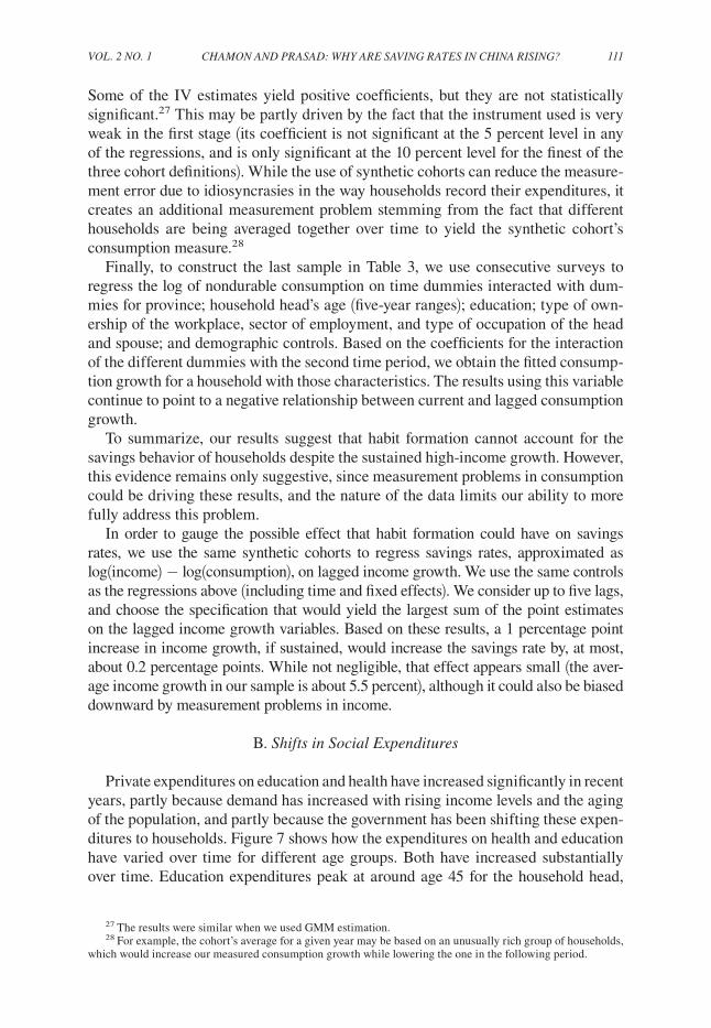
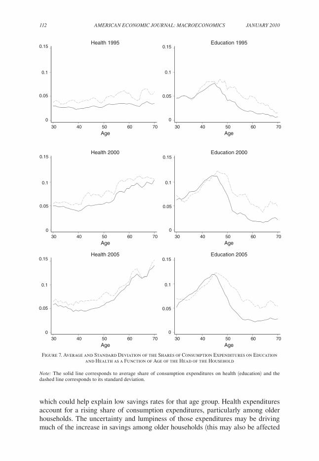
Private expenditures on education and health have increased significantly in recent years, partly because demand has increased with rising income levels and the aging of the population, and partly because the government has been shifting these expen-ditures to households. Figure 7 shows how the expenditures on health and education have varied over time for different age groups. Both have increased substantially over time. Education expenditures peak at around age 45 for the household head,
27 The results were similar when we used GMM estimation.28 For example, the cohort’s average for a given year may be based on an unusually rich group of households,
which would increase our measured consumption growth while lowering the one in the following period.
112 AMERICAN ECONOMIC JOURNAL: MACROECONOMICS JANUARY 2010
which could help explain low savings rates for that age group. Health expenditures account for a rising share of consumption expenditures, particularly among older households. The uncertainty and lumpiness of those expenditures may be driving much of the increase in savings among older households (this may also be affected
0
0.05
0.1
0.15
30 40 50 60 70Age
Health 1995
30 40 50 60 70Age
Education 1995
30 40 50 60 70Age
Health 2000
30 40 50 60 70Age
Education 2000
30 40 50 60 70Age
Health 2005
30 40 50 60 70Age
Education 2005
0
0.05
0.1
0.15
0
0.05
0.1
0.15
0
0.05
0.1
0.15
0
0.05
0.1
0.15
0
0.05
0.1
0.15
Figure 7. Average and Standard Deviation of the Shares of Consumption Expenditures on Education and Health as a Function of Age of the Head of the Household
Note: The solid line corresponds to average share of consumption expenditures on health (education) and the dashed line corresponds to its standard deviation.
VOL. 2 NO. 1 113CHAMON AND PRASAD: WHY ARE SAVING RATES IN CHINA RISING?
by a selection bias, whereby elders who remain heads of households are, on average, better off, and have a higher demand for private health care).29
The fraction of households in our sample for which health expenditures exceed 20 percent of total consumption expenditures (a reasonable threshold for measuring the risk of large private health expenditures) has risen from 1 percent in 1995 to 7 percent in 2005. To examine the vulnerability of older households, we constructed a dummy equal to one if health expenditures exceed this threshold. We then estimate a probit for that variable, using, as predictors, the log of nonhealth consumption expenditures, demographic controls, and province and year dummies. Our measure of a household’s vulnerability to health risk equals 1 if the fitted probability exceeds 10 percent. For households with at least one individual above the age of 60, this measure of vulnerability to health shocks jumps from 0.3 percent in 1995 to 19.1 per-cent in 2005. We also find that the share of total expenditures devoted to education expenditures is highest for households with children in the 15–19 age range (after controlling for compositional and other characteristics of the household). Adding one child in this age range to a two-person household increases the share of educa-tion expenditures in total expenditures by about 5 percentage points in 1995. This marginal effect increases to nearly 8 percentage points by 2005. In Section V, we will formally investigate the effects of these factors on household savings.
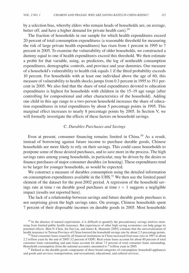
C. Durables Purchases and Savings
Even at present, consumer financing remains limited in China.30 As a result, instead of borrowing against future income to purchase durable goods, Chinese households are more likely to rely on their savings. This could cause households to postpone some of those desired purchases, and to save more in the process. The high savings rates among young households, in particular, may be driven by the desire to finance purchases of major consumer durables (or housing). These expenditures tend to be larger for younger households, as would be expected.
We construct a measure of durables consumption using the detailed information on consumption expenditures available in the UHS.31 We then use the limited panel element of the dataset for the post-2002 period. A regression of the household sav-ings rate at time t on durable good purchases at time t + 1 suggests a negligible impact (results not reported here).
The lack of a relationship between savings and future durable goods purchases is not surprising given the high savings rates. On average, Chinese households spent 7 percent of their disposable incomes on durable goods in 2005. Most households
29 In the absence of natural experiments, it is difficult to quantify the precautionary savings motives stem-ming from limited public health insurance. But experiences of other high saving economies can help gauge its potential effects. Shin-Yi Chou, Jin-Tan Liu, and James K. Hammitt (2003) estimate that the universalization of health insurance in Taiwan Province of China lowered the household savings rate by about 2.5 percentage points.
30 Total consumer loans issued by all financial institutions in China increased from near zero in 1997 to about 2.2 trillion yuan by the end of 2005 (12 percent of GDP). Real estate loans account for about 80 percent of total consumer loans outstanding and auto loans account for about 7.5 percent of total consumer loans outstanding. Household consumption (from the national accounts) amounted to 7 trillion yuan in 2005.
31 Defined as the durable goods components of three broad categories of consumption: household appliances and goods and services; transportation; and recreational, educational, and cultural services.
114 AMERICAN ECONOMIC JOURNAL: MACROECONOMICS JANUARY 2010
could have financed such purchases just by saving less during that year, without needing to draw on past savings. In 2005, the ninety-fifth percentile of the ratio of durables purchases to disposable income was 20 percent, so only the largest (and rare) purchases would require a depletion of past savings. Moreover, since a signifi-cant share of Chinese households’ wealth is in liquid assets, such as bank deposits, even large purchases could be financed by drawing on those liquid savings.
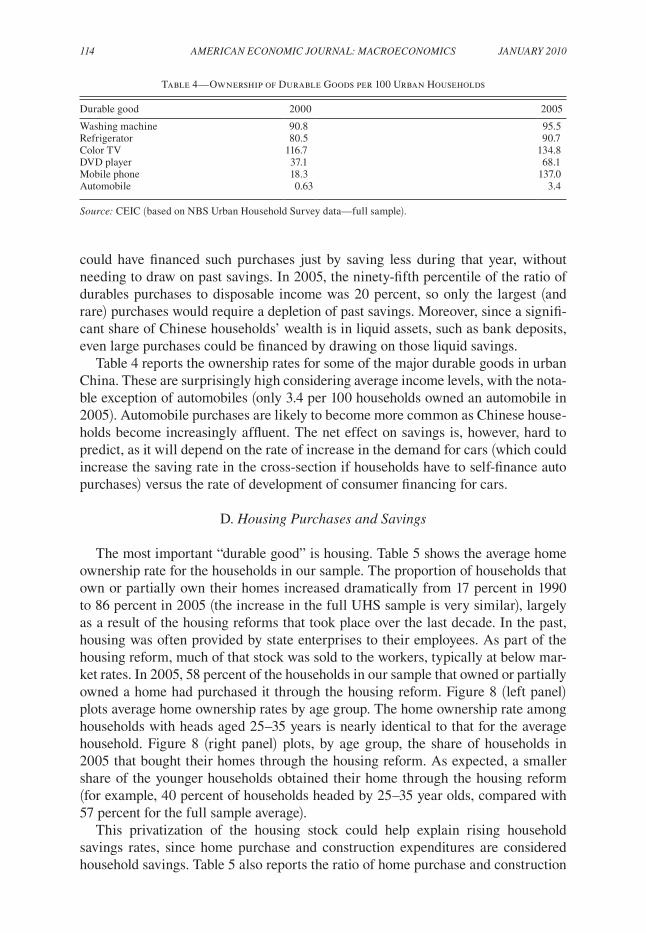
Table 4 reports the ownership rates for some of the major durable goods in urban China. These are surprisingly high considering average income levels, with the nota-ble exception of automobiles (only 3.4 per 100 households owned an automobile in 2005). Automobile purchases are likely to become more common as Chinese house-holds become increasingly affluent. The net effect on savings is, however, hard to predict, as it will depend on the rate of increase in the demand for cars (which could increase the saving rate in the cross-section if households have to self-finance auto purchases) versus the rate of development of consumer financing for cars.
D. Housing Purchases and Savings
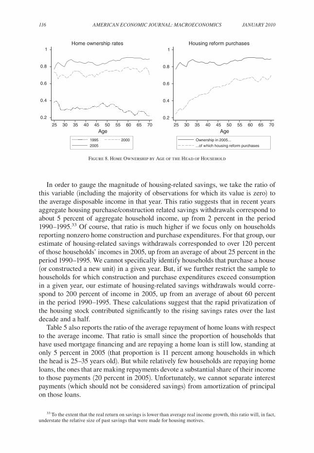
The most important “durable good” is housing. Table 5 shows the average home ownership rate for the households in our sample. The proportion of households that own or partially own their homes increased dramatically from 17 percent in 1990 to 86 percent in 2005 (the increase in the full UHS sample is very similar), largely as a result of the housing reforms that took place over the last decade. In the past, housing was often provided by state enterprises to their employees. As part of the housing reform, much of that stock was sold to the workers, typically at below mar-ket rates. In 2005, 58 percent of the households in our sample that owned or partially owned a home had purchased it through the housing reform. Figure 8 (left panel) plots average home ownership rates by age group. The home ownership rate among households with heads aged 25–35 years is nearly identical to that for the average household. Figure 8 (right panel) plots, by age group, the share of households in 2005 that bought their homes through the housing reform. As expected, a smaller share of the younger households obtained their home through the housing reform (for example, 40 percent of households headed by 25–35 year olds, compared with 57 percent for the full sample average).
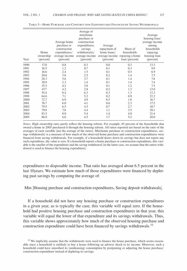
This privatization of the housing stock could help explain rising household savings rates, since home purchase and construction expenditures are considered household savings. Table 5 also reports the ratio of home purchase and construction
Table 4—Ownership of Durable Goods per 100 Urban Households
Durable good 2000 2005
Washing machine 90.8 95.5Refrigerator 80.5 90.7Color TV 116.7 134.8DVD player 37.1 68.1Mobile phone 18.3 137.0Automobile 0.63 3.4
Source: CEIC (based on NBS Urban Household Survey data—full sample).
VOL. 2 NO. 1 115CHAMON AND PRASAD: WHY ARE SAVING RATES IN CHINA RISING?
expenditures to disposable income. That ratio has averaged about 6.5 percent in the last 10years. We estimate how much of those expenditures were financed by deplet-ing past savings by computing the average of:
Min [Housing purchase and construction expenditures, Saving deposit withdrawals].
If a household did not have any housing purchase or construction expenditures in a given year, as is typically the case, this variable will equal zero. If the house-hold had positive housing purchase and construction expenditures in that year, this variable will equal the lower of that expenditure and its savings withdrawals. Thus, this variable shows approximately how much of the observed housing purchase and construction expenditure could have been financed by savings withdrawals.32
32 We implicitly assume that the withdrawals were used to finance the house purchase, which seems reason-able since a household is unlikely to buy a house following an adverse shock to its income. Moreover, such a household could have smoothed its (nonhousing) consumption by postponing or adjusting the house purchase/construction expenditure instead of depleting its savings.
Table 5—Home Purchase and Construction Expenditures Financed by Saving Withdrawals
Year
Home ownership (percent)
Average home purchase or construction
expenditures/average income
(percent)
Average of min(home
purchase or construction expenditures,
savings withdrawals)/
average income (percent)
Average repayment of home loans/
average income (percent)
Share of households
repaying a home loan (percent)
Average housing loan/
average income among
households repaying
housing loan (percent)
1990 17.0 0.8 0.3 0.0 0.3 13.31991 18.5 1.2 0.7 0.1 0.3 9.91992 16.6 2.4 1.5 0.1 0.5 6.91993 20.6 3.8 2.5 0.2 1.4 7.51994 28.3 5.6 3.7 0.1 1.4 7.61995 30.9 2.3 1.4 0.1 1.4 7.41996 35.5 4.2 3.0 0.1 1.2 7.51997 47.7 4.2 2.8 0.2 1.3 13.01998 55.4 8.4 6.3 0.3 1.3 12.31999 64.6 7.1 5.2 0.2 0.9 22.22000 72.7 6.9 4.9 0.5 1.8 16.72001 76.7 6.0 4.1 0.6 2.3 17.52002 79.5 6.5 4.5 0.7 2.7 18.72003 79.9 7.0 4.4 1.1 3.5 20.12004 83.5 8.0 5.4 1.4 4.0 21.42005 86.0 6.6 4.5 1.7 5.2 20.0
Notes: High ownership rates partly reflect the housing reform. For example, 65 percent of the households that owned a home in 2005 purchased it through the housing reform. All ratios reported are based on the ratio of the averages of each variable (not the average of the ratios). Min(home purchase or construction expenditures, sav-ings withdrawals) is a measure of how much of the observed home purchase and construction expenditures were financed from saving withdrawals. For example, if a household draws down its savings but does not report any such expenditure, the value is zero. If a household reports a home purchase or construction expenditure, this vari-able is the smaller of the expenditure and the saving withdrawal (in the latter case, we assume that the entire with-drawal is used to finance the housing expenditure).
116 AMERICAN ECONOMIC JOURNAL: MACROECONOMICS JANUARY 2010
In order to gauge the magnitude of housing-related savings, we take the ratio of this variable (including the majority of observations for which its value is zero) to the average disposable income in that year. This ratio suggests that in recent years aggregate housing purchase/construction related savings withdrawals correspond to about 5 percent of aggregate household income, up from 2 percent in the period 1990–1995.33 Of course, that ratio is much higher if we focus only on households reporting nonzero home construction and purchase expenditures. For that group, our estimate of housing-related savings withdrawals corresponded to over 120 percent of those households’ incomes in 2005, up from an average of about 25 percent in the period 1990–1995. We cannot specifically identify households that purchase a house (or constructed a new unit) in a given year. But, if we further restrict the sample to households for which construction and purchase expenditures exceed consumption in a given year, our estimate of housing-related savings withdrawals would corre-spond to 200 percent of income in 2005, up from an average of about 60 percent in the period 1990–1995. These calculations suggest that the rapid privatization of the housing stock contributed significantly to the rising savings rates over the last decade and a half.
Table 5 also reports the ratio of the average repayment of home loans with respect to the average income. That ratio is small since the proportion of households that have used mortgage financing and are repaying a home loan is still low, standing at only 5 percent in 2005 (that proportion is 11 percent among households in which the head is 25–35 years old). But while relatively few households are repaying home loans, the ones that are making repayments devote a substantial share of their income to those payments (20 percent in 2005). Unfortunately, we cannot separate interest payments (which should not be considered savings) from amortization of principal on those loans.
33 To the extent that the real return on savings is lower than average real income growth, this ratio will, in fact, understate the relative size of past savings that were made for housing motives.
0.2
0.4
0.6
0.8
1
25 30 35 40 45 50 55 60 65 70
Age
1995 2000
2005
Home ownership rates
25 30 35 40 45 50 55 60 65 70
Age
Ownership in 2005...
...of which housing reform purchases
Housing reform purchases
0.2
0.4
0.6
0.8
1
Figure 8. Home Ownership by Age of the Head of Household
VOL. 2 NO. 1 117CHAMON AND PRASAD: WHY ARE SAVING RATES IN CHINA RISING?
If home ownership motives have been an important contributor to savings, the high ownership rates that have now been attained point to a potential decline in sav-ings rates in the near future. But anecdotal evidence suggests that many households would like to upgrade their living conditions (which seems particularly relevant for owners of older units obtained through the housing reform) and that, despite the high home ownership rate, the housing market in China remains very active. We explore the empirical implications in Section V. This discussion indicates that developments in mortgage markets could affect household savings behavior. Perhaps more impor-tantly, if households were able to tap their illiquid housing wealth, the need for precautionary savings would decline (since, in the event of an adversity, households would be able to borrow against their housing equity, using the house as collateral).
E. Effects of State Enterprise Restructuring on Saving Behavior
Increased precautionary saving due to uncertainties stemming from China’s tran-sition to a market economy could potentially help explain the increase in saving.34 The high savings rates among young households may be driven by the need to build an adequate buffer stock of savings to smooth adverse shocks to their income. This factor could also explain why we find that the higher saving cohorts are those that were in their 40s and 50s in 1990. These cohorts bore much of the increase in uncer-tainty related to the move toward a market economy, and do not have as many years of rapid income growth ahead as the younger cohorts to reap the benefits of those reforms. Moreover, they may have found themselves in a situation where their past savings were no longer appropriate in an environment of increased uncertainty, and, as a result, had to re-evaluate their savings plans and make up for past savings that were not made.
It is difficult to quantify the magnitude of the effect of uncertainty on savings using repeated cross-sections of micro data, however, since that increase in aggregate uncertainty affects all households (and we need some variation across households in order to identify an effect). But insights can be obtained by analyzing variations in saving behavior across different groups of households that faced different dimen-sions of this “transition risk.”
One relevant dimension is based on State-Owned Enterprise (SOE) employment. In most economies, SOE employment is likely to be more stable so, all else being equal, workers employed in the state sector should save less. In the case of China, concerns related to SOE reforms could have contributed to an increase in savings rates of households reliant on SOE labor income relative to other households. An implicit assumption underlying this argument is that, while the level of uncer-tainty may be higher in the private sector and overall macro uncertainty may have increased, the relative increase in uncertainty has been greater for SOE employees.35
34 Nicola Fuchs-Schündeln (2008) finds that the precautionary motive plays an important role in explaining the saving behavior of East German households around the time of German reunification.
35 Prior to the SOE reforms, workers received a number of housing, health, education, and pension benefits through their employer. As some benefits are reduced, or their future becomes more uncertain due to SOE restruc-turing, households have stronger motives to save.
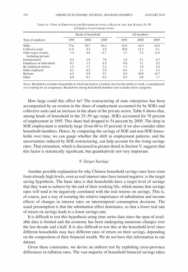
118 AMERICAN ECONOMIC JOURNAL: MACROECONOMICS JANUARY 2010
How large could this effect be? The restructuring of state enterprises has been accompanied by an erosion in the share of employment accounted for by SOEs and collective units and an increase in the share of the private sector. Table 6 shows that, among heads of household in the 25–59 age range, SOEs accounted for 78 percent of employment in 1995. This share had dropped to 54 percent by 2005. The drop in SOE employment is similarly large (from 68 to 43 percent) if we also consider other household members. Hence, by comparing the savings of SOE and non-SOE house-holds over time, we can gauge whether the shift in employment patterns, and the uncertainties induced by SOE restructuring, can help account for the rising savings rates. That estimation, which is discussed in greater detail in Section V, suggests that this factor is statistically significant, but quantitatively not very important.
F. Target Savings
Another possible explanation for why Chinese household savings rates have risen from already high levels, even as real interest rates have turned negative, is the target saving hypothesis. The basic idea is that households have a target level of savings that they want to achieve by the end of their working life, which means that savings rates will tend to be negatively correlated with the real returns on savings. This is, of course, just a way of restating the relative importance of substitution and income effects of changes in interest rates on intertemporal consumption decisions. The usual presumption is that the substitution effect dominates, so that a lower real rate of return on savings leads to a lower savings rate.
It is difficult to test this hypothesis using time series data since the span of avail-able data is limited and the economy has been undergoing numerous changes over the last decade and a half. It is also difficult to test this at the household level since different households may face different rates of return on their savings, depending on the composition of their financial wealth. We do not have this information in our dataset.
Given these constraints, we devise an indirect test by exploiting cross-province differences in inflation rates. The vast majority of household financial savings takes
Table 6—Type of Employer for Households with a Head in the Age Range 25–59 (all figures in percentage terms)
Heads of household All members
Type of employer 1995 2000 2005 1995 2000 2005
SOEs 77.6 70.7 54.4 67.8 61.9 42.9Collective units 11.9 9.3 4.5 18.0 12.2 6.1Other types of units (including private)
1.5 4.6 11.7 1.7 5.3 11.9
Entrepreneurs 0.5 2.9 7.8 1.0 3.1 6.7Employees of individuals 0.3 1.3 6.5 0.8 3.1 9.2Re-employed retirees 1.5 1.7 2.3 1.3 1.8 2.6Other employed 0.1 0.5 2.9 0.4 1.1 4.3Retirees 6.5 8.8 9.7 8.5 10.9 14.7Other 0.0 0.1 0.2 0.5 0.6 1.7
Notes: Breakdown excludes households in which the head is a student, has lost the ability to work, is unemployed, or is waiting for an assignment. Breakdown among household members also excludes those categories.
VOL. 2 NO. 1 119CHAMON AND PRASAD: WHY ARE SAVING RATES IN CHINA RISING?
the form of bank deposits and, since the deposit rate is fixed by the central bank, all households face the same nominal rate of return on their savings. Thus, inflation differentials across provinces can be interpreted as a proxy for differences in real interest rates.
We use published UHS data on per capita income and consumption averages for 31 mainland provinces/municipalities for the period 1992–2006 (yielding a total of 421 observations). We regress the provincial/municipality average savings rate on the log of the average disposable income, the ex-post one-year-ahead inflation rate, province dummies, and year dummies (to capture differences in the nominal interest rate across years and trends in savings). Our estimates indicate that a 1 percentage point increase in the 1-year-ahead ex-post inflation rate is associated with an increase of 0.24 percentage points (standard error: 0.08) in the household savings rate. This correlation provides some indirect support for the view that lower real interest rates are associated with higher savings rates.36 We re-estimated the regression using our 10-province sample, which yields similar results (0.22; standard error: 0.13).
These results should, of course, be interpreted with caution, as there are other rea-sons why expected inflation could affect savings. Furthermore, by construction, we can tease out only a cross-province effect rather than an aggregate nationwide effect of a change in interest rates on savings. Even if taken at face value, our point esti-mates suggest that the effect is not quantitatively important. For example, based on the province-level results, it would take an inflation rate 4 percentage points above the national average in that year to raise provincial saving rates by 1 percentage point. Thus, even if our estimated correlation held up at the national level, it would not explain the large (and rising) household national saving rates. Hence, we do not pursue this further here. Nevertheless, we find it intriguing that, based on our rather crude and indirect test, we cannot refute the target savings hypothesis altogether.
V. A Composite Sketch
We now develop an estimation framework for jointly analyzing the importance of some of the key hypotheses in driving the increase in the household savings rate. The evidence in Section IV suggests that savings for durables purchases, consump-tion persistence due to habit formation, and target savings behavior are not major contributors to this increase. Hence, we begin by focusing on the other motives for saving that seem quantitatively most relevant: housing purchases, shifts in social expenditures, and SOE restructuring.
We estimate composite median regressions (quantile regressions estimated at the median) for the household savings rate using the following controls.
Demographics.—Dummies are for the age of the head of household being 25–29, 30–34, … , 60–64, and 65–69 years old; the log of the household size; and the share of household members aged 0–4, 5–9, 10–14, 15–19, 20–59, and 60 or above. These controls can inform us about how the presence of elderly persons and children of
36 Detailed estimation results are available from the authors. The estimated coefficient on the log of disposable income is 0.16, which is in line with the other estimates in this paper.
120 AMERICAN ECONOMIC JOURNAL: MACROECONOMICS JANUARY 2010
different ages affect savings, helping us to gauge savings motives related to future expenditures on health and education.
Income.—The log of disposable income. We also include dummies for the educa-tion, occupation, and industry of the household head and the spouse (if present), and province and year dummies. These dummies can capture, among other things, the permanent income of a household with given characteristics. Thus, when reading the coefficient on log income, one should bear in mind that the estimated effect includes these other controls.
SOE Employment.—This effect is captured by two dummies. The first equals one if there is one SOE employee in the household, and the second equals one if there are two or more SOE employees in the household. This specification allows us to capture possible nonlinearities in the effect—i.e., for a given level of income, the marginal effect could be different depending on whether some or all of the house-hold’s labor income comes from the SOE sector.37
Home Ownership.—A dummy equal to one if the household owns its dwelling.
Health Risk.—The measure of vulnerability to large health expenditures described in Section IVB. It is essentially a dummy variable that takes the value unity if the fitted probability (from a first-stage probit) of a large health expenditure exceeds 10 percent.38
Table 7 presents the regression results. To abstract from year-to-year variations, we present results for the following periods: 1992–1996, 1997–2001, and 2002–2005. For each period, we present the results from a specification including only the income and demographic controls (and also year and province dummies), and then a second specification that also controls for SOE employment, home ownership, and health expenditure risk. Since we use fitted values of the health expenditure risk as a control in these regressions, we bootstrap the data in both stages to adjust the stan-dard errors in the relevant specifications of this table.
It is worth noting that the estimated year dummies (not reported in the table for presentation purposes) do not imply a rising trend. That is, changes in the variables that we consider in our regressions can explain the rising savings rate. For example, if we drop year dummies altogether, the fitted values from specification (1) would imply a median savings rate of 24 percent in 2005, which is slightly above the level of 22 percent observed in the data.
37 The results that we report here were similar if, instead of these dummies for SOE employment, we used the share of household income from SOE earnings as a regressor. Fuchs-Schündeln and Schündeln (2005) note that differences in risk aversion could result in self-selection into occupations with different risk characteristics, which could affect estimates of precautionary saving behavior.
38 Note that this dummy structure is more appropriate than adding the fitted probability as a control in the main regression, since the latter’s effect is nonlinear (once a household faces a sufficiently high probability of that risk, it should start provisioning for it). It is possible that households start saving in advance of health risk but, since such anticipatory behavior is likely to be closely correlated with age, we cannot disentangle it from the overall life-cycle effects that we estimate with age dummies.
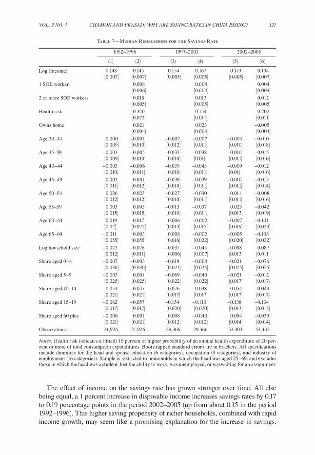
VOL. 2 NO. 1 121CHAMON AND PRASAD: WHY ARE SAVING RATES IN CHINA RISING?
The effect of income on the savings rate has grown stronger over time. All else being equal, a 1 percent increase in disposable income increases savings rates by 0.17 to 0.19 percentage points in the period 2002–2005 (up from about 0.15 in the period 1992–1996). This higher saving propensity of richer households, combined with rapid income growth, may seem like a promising explanation for the increase in savings.
Table 7—Median Regressions for the Savings Rate
1992–1996 1997–2001 2002–2005
(1) (2) (3) (4) (5) (6)
Log (income) 0.148 0.145 0.154 0.167 0.173 0.194[0.007] [0.007] [0.005] [0.005] [0.005] [0.007]
1 SOE worker 0.008 0.004 0.004[0.006] [0.004] [0.004]
2 or more SOE workers 0.018 0.013 0.012[0.005] [0.005] [0.005]
Health risk 0.320 0.154 0.202[0.073] [0.011] [0.011]
Owns home 0.021 0.023 –0.005[0.004] [0.004] [0.004]
Age 30–34 0.000 –0.001 –0.007 –0.007 –0.003 –0.010[0.009] [0.010] [0.012] [0.011] [0.010] [0.018]
Age 35–39 –0.003 –0.005 –0.037 –0.038 –0.010 –0.015[0.009] [0.010] [0.010] [0.01] [0.011] [0.016]
Age 40–44 –0.003 –0.006 –0.039 –0.043 –0.009 –0.012[0.010] [0.011] [0.010] [0.011] [0.01] [0.016]
Age 45–49 0.003 0.001 –0.039 –0.039 –0.010 –0.013[0.011] [0.012] [0.010] [0.011] [0.011] [0.014]
Age 50–54 0.026 0.023 –0.027 –0.030 0.011 –0.008[0.012] [0.012] [0.010] [0.011] [0.011] [0.016]
Age 55–59 0.003 0.005 –0.013 –0.037 0.023 –0.042[0.015] [0.015] [0.010] [0.011] [0.013] [0.019]
Age 60–64 0.019 0.017 0.006 –0.002 –0.007 –0.101[0.02] [0.022] [0.013] [0.015] [0.019] [0.029]
Age 65–69 –0.011 0.003 0.008 –0.002 –0.005 –0.108[0.055] [0.055] [0.016] [0.022] [0.020] [0.032]
Log household size –0.072 –0.076 –0.037 –0.045 –0.098 –0.087[0.012] [0.011] [0.006] [0.007] [0.013] [0.011]
Share aged 0–4 –0.007 –0.003 –0.019 –0.004 –0.021 –0.076[0.030] [0.030] [0.023] [0.023] [0.025] [0.025]
Share aged 5–9 –0.003 0.001 –0.069 –0.040 –0.021 –0.012[0.025] [0.025] [0.022] [0.022] [0.017] [0.017]
Share aged 10–14 –0.053 –0.047 –0.076 –0.038 –0.054 –0.043[0.021] [0.021] [0.017] [0.017] [0.017] [0.017]
Share aged 15–19 –0.062 –0.057 –0.154 –0.113 –0.138 –0.134[0.017] [0.017] [0.020] [0.020] [0.013] [0.013]
Share aged 60 plus –0.006 0.001 0.008 –0.040 0.054 –0.039[0.021] [0.021] [0.012] [0.012] [0.014] [0.014]
Observations 21,926 21,926 29,366 29,366 53,403 53,403
Notes: Health risk indicates a (fitted) 10 percent or higher probability of an annual health expenditure of 20 per-cent or more of total consumption expenditures. Bootstrapped standard errors are in brackets. All specifications include dummies for the head and spouse education (6 categories), occupation (9 categories), and industry of employment (16 categories). Sample is restricted to households in which the head was aged 25–69, and excludes those in which the head was a student, lost the ability to work, was unemployed, or waswaiting for an assignment.
122 AMERICAN ECONOMIC JOURNAL: MACROECONOMICS JANUARY 2010
But, one should bear in mind that this coefficient is capturing the effect of income after controlling for a host of household characteristics (e.g., education, occupation, prov-ince, and year, among others), so one cannot simply multiply this coefficient by income growth to read an effect on the savings rate. But, this rising coefficient does suggest that, all else being equal, households tend to save more of the idiosyncratic compo-nents of their income, which is consistent with stronger precautionary saving motives.
The age dummies confirm that households with relatively very young or very old heads tend to save more, although the magnitude of the difference in savings is more muted than the age effects estimated in Section III. This suggests other controls may be capturing the differences by age shown in those plots (for example, high savings among the young being partly captured by their higher income levels). One striking feature of our results is how strongly the introduction of the health risk variable affects the demographic controls related to old age in the 2002–2005 sample. For example, the results in column 5 indicate that a household consisting of two adults in the age range of 65–69 would have saved, all else equal, 5 percentage points more than a household consisting of two adults in the age range of 25–29. But in the specification with the health risk control (column 6), the difference due to the demo-graphic dummies goes from plus 5 percentage points to minus 14 percentage points.
The reason for this change is that the health risk dummy (which mainly applies to older households) has almost a 20 percentage point effect on the savings rate.39 Once we factor in the effect of the health risk on savings, an older household for which that risk is present will still save 5 percentage points more of its income than the younger household (i.e., this control does not alter the fact that the elderly save more. It just attributes that higher savings to a health motive as opposed to demographic controls). While the magnitude of the coefficient on health risk in column 6 is actually compara-ble to the one in the earlier samples (columns 2 and 4), the importance of that variable in the 1992–1996 sample is, in fact, negligible. The health risk dummy was equal to 1 for only 0.2 percent of the households in that period, compared to 8 and 16.8 percent of the households in the period 1997–2001 and 2002–2005, respectively. This explains why the inclusion of that control has such a small effect on elderly savings when going from regression (1) to regression (2), compared to the change from regressions (3) and (4), and, particularly, the large change from regression (5) to regression (6).
While we do not have controls directly related to education expenditures, their importance can be gauged by the household composition controls. For example, we can compare households with children aged 5–9 and 10–14 years with those aged 15–19 for which education expenditures tend to be higher. All else being equal, a 3 person household with one child in the 5–9 age group saved about 2 percentage points more of its income than one with a member in the 15–19 age group in the period 1992–1996, and 4 percentage points more in the period 2002–2005. If we compare the 10–14 age group with the 15–19 age group, the difference is negligible in the period 1992–1996, and it is 3 percentage points in the period 2002–2005.40
39 While we add three additional controls when going from specification (5) to specification (6), the effect on the savings rate of the elderly is driven almost entirely by the health risk control (which is also clear from the magnitudes of the other two controls).
40 For these comparisons, we divide the difference between the respective coefficients on the household com-position dummies by three (since we shift the age group of one member in a three-person household). We chose
VOL. 2 NO. 1 123CHAMON AND PRASAD: WHY ARE SAVING RATES IN CHINA RISING?
This pattern is consistent with higher savings in anticipation of future education expenditures (and with a dip in savings when education expenditures tend to be highest). Note that while education can explain why some households save more than others, the effects on aggregate savings may be muted (as the savings of one group are compensated by the dissavings of the other). This may not be the case for health related savings given the more lumpy and uncertain nature of those expenditures.41
As discussed earlier, we use differentials in savings rates between SOE and non-SOE employees to tease out the magnitude of precautionary motives for saving. Our maintained assumption is that, while overall macro uncertainty has increased and the level of uncertainty may be higher in the private sector, the relative increase in uncertainty has been greater for SOE employees due to restructuring. Having one SOE employee in the household increases the savings rate by almost 1 percentage point in the period 1992–1996, but only by half of a percentage point in the period 2002–2005. Having 2 or more SOE employees raises savings rates by about 2 per-centage points in the first period. In the later periods, that effect declines to about 1 percentage point. This suggests that SOE reforms, by themselves, do not account for a significant portion of the increase in aggregate savings rates. Of course, our results have little to say about the effects of aggregate uncertainty on savings rates. One could argue that, in theory, SOE households should be saving substantially less than their private counterparts, and the fact that they save slightly more, on average, already suggests strong precautionary motives from the reform process. Without knowing what the counterfactual savings rates would have been, however, it is dif-ficult to assess the overall impact of SOE reforms on saving behavior.
Finally, we turn to the home ownership dummy. Households that own their homes save about 2 percentage points more of their income in the period 1992–1996 and 1997–2001 than those that do not own their own homes. The sign is the opposite of what one would expect based on our contention of households saving for house purchases. This effect disappears in the 2002–2005 sample.
Panel A of Table 8 presents estimates for the same regressions as the ones above, but with income and consumption adjusted by an estimated value of owner-occu-pied housing obtained by regressing, for the sample of renters, rent expenditures on nonrent consumption expenditures, demographic controls, and province and SOE employment dummies (since SOE workers often had access to subsidized housing). We then use the fitted values to impute rents for the homeowners. Again, we boot-strap the data (in both stages) to construct the standard errors. We continue to esti-mate a positive effect of home ownership on savings rates in the period 1992–1996 and 1997–2001 (columns 1 and 2), but the effect is now minus 2 percentage points for 2002–2005 (column 3). For comparability with the previous samples, we have used our estimates for the rental values of owner-occupied homes in the period
to use the 5–9 age group rather than the 0–4 age group as the basis for comparison since saving behavior may be atypical following the birth of a child. There has also been an increase in health expenditures among families with small children. The average value of the health expenditure risk dummy in 2005 is 0.38 for families with children aged 0–4, but only 0.09 for families with children aged 5–9. In 1995, those figures were 0.02 and 0.00, respectively. This may explain why the coefficient on the share of household members aged 0–4 becomes so nega-tive in the period 2002–2005 from specification (5) to specification (6).
41 For example, many households may be compelled to accumulate savings, but relatively few may actually get hit by health shocks so the net effect can increase aggregate savings.
124 AMERICAN ECONOMIC JOURNAL: MACROECONOMICS JANUARY 2010
2002–2005, even though those surveys do report imputed rent values. Using the reported, rather than the estimated values, increases the coefficient on the home ownership dummy to minus 1 percentage point (column 5).
The 2002–2005 surveys report an estimated value of the dwellings at market prices. We use that variable to create dummies for value quartiles (by province and year). Column 4 reports the results of a regression including those dummies. Having a home in the bottom quartile raises the savings rate by 1.5 percentage points, and one in the second quartile by 0.3 percentage points. Having a home in the third and top quartiles lowers the savings rate by 1.6 and 3.9 percentage points, respectively (after controlling for income and other household characteristics used in the regres-sion). If we use the imputed rents reported in the 2002–2005 surveys instead of the ones we construct (column 6), the estimated effects of owning a home in the bottom and second quartiles imply increases in the savings rate of 2.4 and 0.8 percentage points, respectively. Owning a home in the third and top quartiles continues to lower the savings rate by 1.4 and 3.9 percentage points, respectively.
As noted in Section IV, anecdotal evidence suggests much of the privatized hous-ing stock is unappealing, and many households may be saving to improve/purchase new dwellings. This is consistent with the results from this last regression, whereby households in higher valued homes save substantially less than those that do not own a home or live in one of low value. Unfortunately, the estimated housing value variable is not available in earlier surveys (so, we cannot test whether this is what is driving the housing-related results in those years).
The effects of home ownership on savings may depend on the age of the house-hold head. For example, a young household head who does not own a dwelling is more likely than a 65 year old to be saving to purchase one. Panel B of Table 8 presents regressions similar to those of panel A, but with interactions of the home ownership dummy with dummies for five-year ranges of the age of the household head (the 25–29 age group dummy is omitted). Home ownership continues to have a positive effect on savings rates in the period 1992–1996, and 1997–2001, although the coefficients on the age interactions are not statistically significant (columns 1–2).
The expected pattern does emerge in the 2002–2005 sample, where home owner-ship implies a large reduction in savings for younger households, but not for older ones (column 3). In that sample, the coefficient on the home ownership dummy is −7.6 percentage points. But the coefficients on its interaction with age are positive, and the combined effect gradually declines as we move from the 25–29 age group toward older households. The point estimates imply effects of −4.7, −3.3, and −2.5 percentage points for 30–34, 35–39, and 40–44-year-old household heads, respec-tively (with the effect for 30–34-year-olds not being statistically significantly differ-ent than the one for 25–29-year-olds). For the 45–49 year old and older age groups, the effect of home ownership on savings seems to fade. The point estimates still imply a negative effect for 50–54-year-old household heads, and a positive effect for the older households (but we cannot reject the hypothesis of zero effect of home ownership on savings among the elderly). The results are similar when the imputed rents reported in the survey are used (column 4).
The results are also similar if we interact the age of the household head with home ownership by housing quartile (not reported in Table 8). Using the fitted imputed
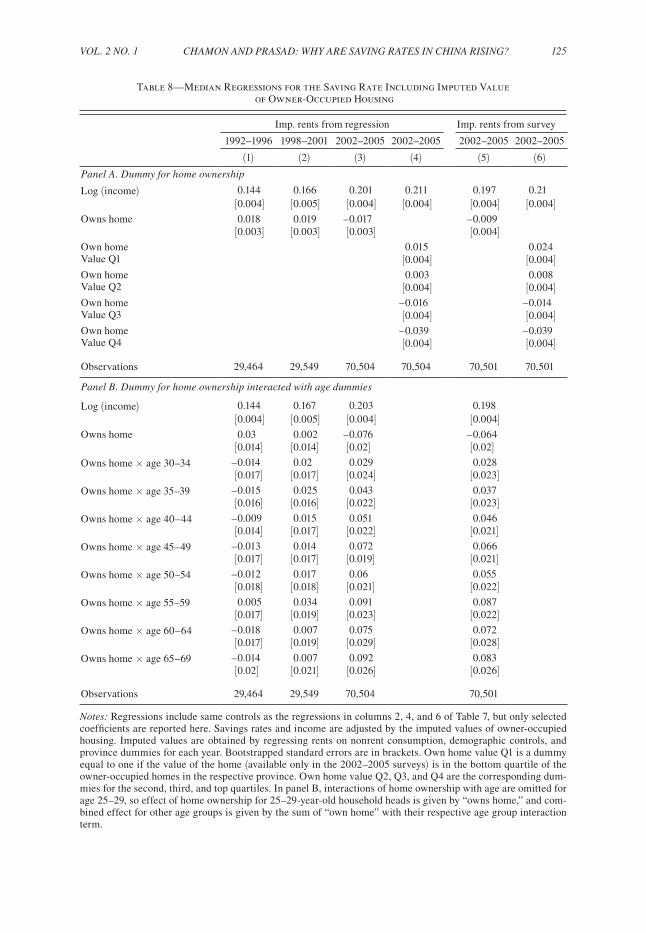
VOL. 2 NO. 1 125CHAMON AND PRASAD: WHY ARE SAVING RATES IN CHINA RISING?
Table 8—Median Regressions for the Saving Rate Including Imputed Value of Owner-Occupied Housing
Imp. rents from regression Imp. rents from survey
1992–1996 1998–2001 2002–2005 2002–2005 2002–2005 2002–2005
(1) (2) (3) (4) (5) (6)Panel A. Dummy for home ownership
Log (income) 0.144 0.166 0.201 0.211 0.197 0.21[0.004] [0.005] [0.004] [0.004] [0.004] [0.004]
Owns home 0.018 0.019 –0.017 –0.009[0.003] [0.003] [0.003] [0.004]
Own home 0.015 0.024Value Q1 [0.004] [0.004]Own home 0.003 0.008Value Q2 [0.004] [0.004]Own home –0.016 –0.014Value Q3 [0.004] [0.004]Own home –0.039 –0.039Value Q4 [0.004] [0.004]
Observations 29,464 29,549 70,504 70,504 70,501 70,501
Panel B. Dummy for home ownership interacted with age dummies
Log (income) 0.144 0.167 0.203 0.198[0.004] [0.005] [0.004] [0.004]
Owns home 0.03 0.002 –0.076 –0.064[0.014] [0.014] [0.02] [0.02]
Owns home × age 30–34 –0.014 0.02 0.029 0.028[0.017] [0.017] [0.024] [0.023]
Owns home × age 35–39 –0.015 0.025 0.043 0.037[0.016] [0.016] [0.022] [0.023]
Owns home × age 40–44 –0.009 0.015 0.051 0.046[0.014] [0.017] [0.022] [0.021]
Owns home × age 45–49 –0.013 0.014 0.072 0.066 [0.017] [0.017] [0.019] [0.021]Owns home × age 50–54 –0.012 0.017 0.06 0.055
[0.018] [0.018] [0.021] [0.022]Owns home × age 55–59 0.005 0.034 0.091 0.087
[0.017] [0.019] [0.023] [0.022]Owns home × age 60–64 –0.018 0.007 0.075 0.072
[0.017] [0.019] [0.029] [0.028]Owns home × age 65–69 –0.014 0.007 0.092 0.083
[0.02] [0.021] [0.026] [0.026]
Observations 29,464 29,549 70,504 70,501
Notes: Regressions include same controls as the regressions in columns 2, 4, and 6 of Table 7, but only selected coefficients are reported here. Savings rates and income are adjusted by the imputed values of owner-occupied housing. Imputed values are obtained by regressing rents on nonrent consumption, demographic controls, and province dummies for each year. Bootstrapped standard errors are in brackets. Own home value Q1 is a dummy equal to one if the value of the home (available only in the 2002–2005 surveys) is in the bottom quartile of the owner-occupied homes in the respective province. Own home value Q2, Q3, and Q4 are the corresponding dum-mies for the second, third, and top quartiles. In panel B, interactions of home ownership with age are omitted for age 25–29, so effect of home ownership for 25–29-year-old household heads is given by “owns home,” and com-bined effect for other age groups is given by the sum of “own home” with their respective age group interaction term.
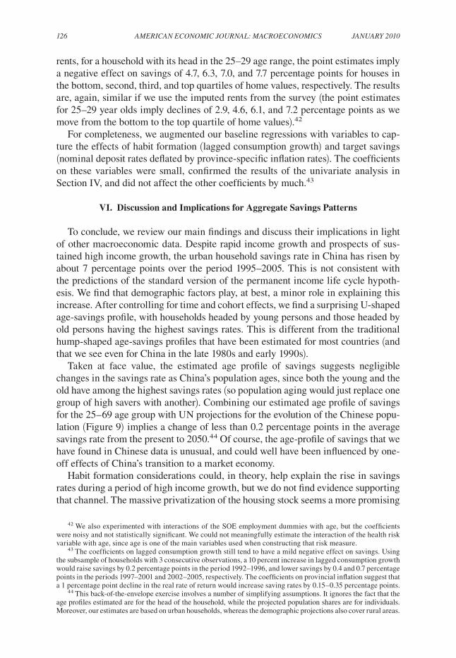
126 AMERICAN ECONOMIC JOURNAL: MACROECONOMICS JANUARY 2010
rents, for a household with its head in the 25–29 age range, the point estimates imply a negative effect on savings of 4.7, 6.3, 7.0, and 7.7 percentage points for houses in the bottom, second, third, and top quartiles of home values, respectively. The results are, again, similar if we use the imputed rents from the survey (the point estimates for 25–29 year olds imply declines of 2.9, 4.6, 6.1, and 7.2 percentage points as we move from the bottom to the top quartile of home values).42
For completeness, we augmented our baseline regressions with variables to cap-ture the effects of habit formation (lagged consumption growth) and target savings (nominal deposit rates deflated by province-specific inflation rates). The coefficients on these variables were small, confirmed the results of the univariate analysis in Section IV, and did not affect the other coefficients by much.43
VI. Discussion and Implications for Aggregate Savings Patterns
To conclude, we review our main findings and discuss their implications in light of other macroeconomic data. Despite rapid income growth and prospects of sus-tained high income growth, the urban household savings rate in China has risen by about 7 percentage points over the period 1995–2005. This is not consistent with the predictions of the standard version of the permanent income life cycle hypoth-esis. We find that demographic factors play, at best, a minor role in explaining this increase. After controlling for time and cohort effects, we find a surprising U-shaped age-savings profile, with households headed by young persons and those headed by old persons having the highest savings rates. This is different from the traditional hump-shaped age-savings profiles that have been estimated for most countries (and that we see even for China in the late 1980s and early 1990s).
Taken at face value, the estimated age profile of savings suggests negligible changes in the savings rate as China’s population ages, since both the young and the old have among the highest savings rates (so population aging would just replace one group of high savers with another). Combining our estimated age profile of savings for the 25–69 age group with UN projections for the evolution of the Chinese popu-lation (Figure 9) implies a change of less than 0.2 percentage points in the average savings rate from the present to 2050.44 Of course, the age-profile of savings that we have found in Chinese data is unusual, and could well have been influenced by one-off effects of China’s transition to a market economy.
Habit formation considerations could, in theory, help explain the rise in savings rates during a period of high income growth, but we do not find evidence supporting that channel. The massive privatization of the housing stock seems a more promising
42 We also experimented with interactions of the SOE employment dummies with age, but the coefficients were noisy and not statistically significant. We could not meaningfully estimate the interaction of the health risk variable with age, since age is one of the main variables used when constructing that risk measure.
43 The coefficients on lagged consumption growth still tend to have a mild negative effect on savings. Using the subsample of households with 3 consecutive observations, a 10 percent increase in lagged consumption growth would raise savings by 0.2 percentage points in the period 1992–1996, and lower savings by 0.4 and 0.7 percentage points in the periods 1997–2001 and 2002–2005, respectively. The coefficients on provincial inflation suggest that a 1 percentage point decline in the real rate of return would increase saving rates by 0.15–0.35 percentage points.
44 This back-of-the-envelope exercise involves a number of simplifying assumptions. It ignores the fact that the age profiles estimated are for the head of the household, while the projected population shares are for individuals. Moreover, our estimates are based on urban households, whereas the demographic projections also cover rural areas.
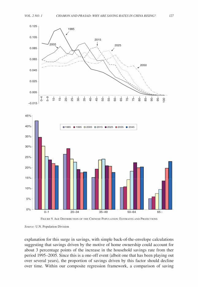
VOL. 2 NO. 1 127CHAMON AND PRASAD: WHY ARE SAVING RATES IN CHINA RISING?
explanation for this surge in savings, with simple back-of-the-envelope calculations suggesting that savings driven by the motive of home ownership could account for about 3 percentage points of the increase in the household savings rate from ther period 1995–2005. Since this is a one-off event (albeit one that has been playing out over several years), the proportion of savings driven by this factor should decline over time. Within our composite regression framework, a comparison of saving
–0.015
0.005
0.025
0.045
0.065
0.085
0.105
0.125
0–4
5–9
10–
15–
20–
25–
30–
35–
40–
45–
50–
55–
60–
65–
70–
75–
80–
85–
90–
95–
100
2005 2025
2015
2050
1985
0%
5%
10%
15%
20%
25%
30%
35%
40%
45%
0–1 20–34 35–49 50–64 65+
Age range
1985 1995 2005 2015 2025 2035 2045
Figure 9. Age Distribution of the Chinese Population: Estimates and Projections
Source: U.N. Population Division
128 AMERICAN ECONOMIC JOURNAL: MACROECONOMICS JANUARY 2010
behavior between households that own their dwellings and those that rent suggests a more limited effect of this factor. It comes out clearly only when we make a distinc-tion between households with younger and older heads, or between owners of high-value and low-value homes (the latter may save to upgrade to better homes).
The increasing private burden of education and health expenditures seems among the strongest candidates for explaining the increase in savings rates, at least during a transition period. Our estimates show that health expenditure-related risks can largely explain the dramatic increase in savings rates among elderly households. The uncertainty related to those expenditures can also increase aggregate savings rates despite the higher consumption expenditures of the households suffering an adverse health shock.45 Our estimates suggest that the elimination of the risk of health expenditures exceeding 20 percent of income (through a catastrophic insur-ance scheme) would have lowered the median savings rate in 2005 by 3.5 percentage points, assuming no behavioral responses to such a scheme. Differences in saving behavior by households with children of different ages are consistent with expected future education expenditures increasing savings (or at least lowering consumption).
The effects of these shifts, together with precautionary motives stemming from state enterprise restructuring and market-oriented reforms, should eventually fade as households adjust their consumption plans and build up a level of assets appropri-ate for this post-transition environment. This build-up in savings could have been smaller if financial markets were more developed. Financial frictions also strengthen precautionary savings motives, and borrowing constraints can play an important role in driving up savings rates despite rapid income growth, especially among younger households. Finally, we also found some weak indirect evidence in support of the “target saving” hypothesis, whereby Chinese households have high savings rates because they are targeting a certain level of wealth and the real return on their savings, most of which goes into bank deposits, is small (and has recently become negative).
What are the implications of our findings for the debate about how to “rebalance” China’s growth by boosting domestic consumption? As financial markets develop, households should benefit from being able to borrow against future income, better opportunities for portfolio diversification, and better rates of return on their savings. Improvements in the social safety net would pool the risks associated with idiosyn-cratic income shocks and health expenditures, reducing the need for households to save in order to self-insure against these risks. Increasing public provision of education could also lower household savings by reducing the need to accumulate assets to finance future education expenditures. Thus, policies that foster financial sector development and increased social expenditures could play an important role in helping to smooth consumption over the life cycle (Blanchard and Giavazzi 2006). This would moderate household savings rates and help in rebalancing growth toward consumption.
45 During the transition to a steady state with a higher level of savings for these reasons, the short-run cross-sectional dynamics would imply an increase in savings as most households would have net savings, with only a small fraction of them drawing down their savings to meet these expenditures
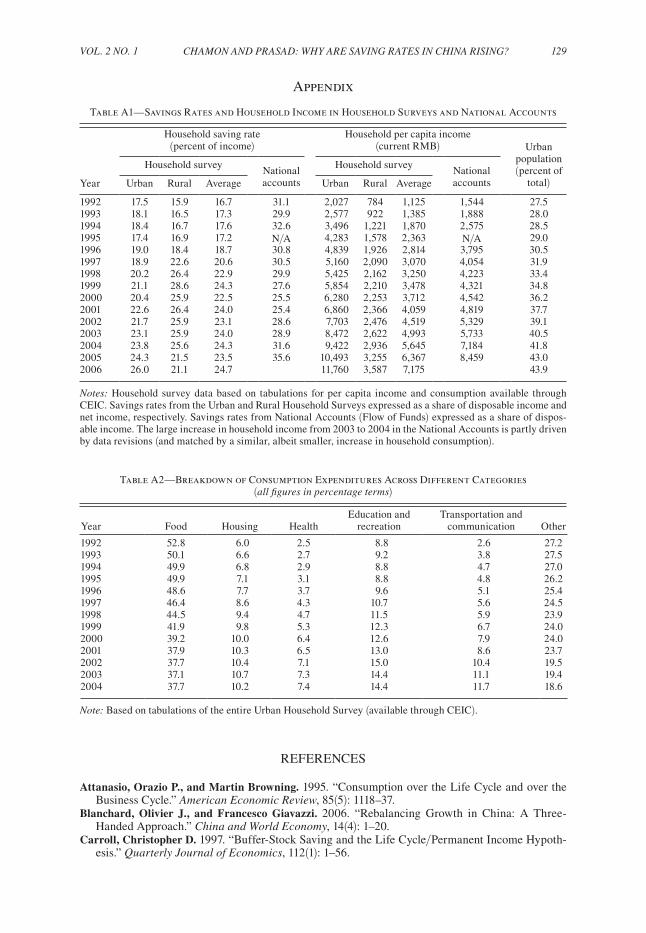
VOL. 2 NO. 1 129CHAMON AND PRASAD: WHY ARE SAVING RATES IN CHINA RISING?
Appendix
REFERENCES
Attanasio, Orazio P., and Martin Browning. 1995. “Consumption over the Life Cycle and over the Business Cycle.” American Economic Review, 85(5): 1118–37.
Blanchard, Olivier J., and Francesco Giavazzi. 2006. “Rebalancing Growth in China: A Three-Handed Approach.” China and World Economy, 14(4): 1–20.
Carroll, Christopher D. 1997. “Buffer-Stock Saving and the Life Cycle/Permanent Income Hypoth-esis.” Quarterly Journal of Economics, 112(1): 1–56.
Table A1—Savings Rates and Household Income in Household Surveys and National Accounts
Household saving rate(percent of income)
Household per capita income(current RMB) Urban
population(percent of
total)Household survey
Nationalaccounts
Household surveyNationalaccountsYear Urban Rural Average Urban Rural Average
1992 17.5 15.9 16.7 31.1 2,027 784 1,125 1,544 27.51993 18.1 16.5 17.3 29.9 2,577 922 1,385 1,888 28.01994 18.4 16.7 17.6 32.6 3,496 1,221 1,870 2,575 28.51995 17.4 16.9 17.2 N/A 4,283 1,578 2,363 N/A 29.01996 19.0 18.4 18.7 30.8 4,839 1,926 2,814 3,795 30.51997 18.9 22.6 20.6 30.5 5,160 2,090 3,070 4,054 31.91998 20.2 26.4 22.9 29.9 5,425 2,162 3,250 4,223 33.41999 21.1 28.6 24.3 27.6 5,854 2,210 3,478 4,321 34.82000 20.4 25.9 22.5 25.5 6,280 2,253 3,712 4,542 36.22001 22.6 26.4 24.0 25.4 6,860 2,366 4,059 4,819 37.72002 21.7 25.9 23.1 28.6 7,703 2,476 4,519 5,329 39.12003 23.1 25.9 24.0 28.9 8,472 2,622 4,993 5,733 40.52004 23.8 25.6 24.3 31.6 9,422 2,936 5,645 7,184 41.82005 24.3 21.5 23.5 35.6 10,493 3,255 6,367 8,459 43.02006 26.0 21.1 24.7 11,760 3,587 7,175 43.9
Notes: Household survey data based on tabulations for per capita income and consumption available through CEIC. Savings rates from the Urban and Rural Household Surveys expressed as a share of disposable income and net income, respectively. Savings rates from National Accounts (Flow of Funds) expressed as a share of dispos-able income. The large increase in household income from 2003 to 2004 in the National Accounts is partly driven by data revisions (and matched by a similar, albeit smaller, increase in household consumption).
Table A2—Breakdown of Consumption Expenditures Across Different Categories (all figures in percentage terms)
Year Food Housing HealthEducation and
recreationTransportation and
communication Other
1992 52.8 6.0 2.5 8.8 2.6 27.21993 50.1 6.6 2.7 9.2 3.8 27.51994 49.9 6.8 2.9 8.8 4.7 27.01995 49.9 7.1 3.1 8.8 4.8 26.21996 48.6 7.7 3.7 9.6 5.1 25.41997 46.4 8.6 4.3 10.7 5.6 24.51998 44.5 9.4 4.7 11.5 5.9 23.91999 41.9 9.8 5.3 12.3 6.7 24.02000 39.2 10.0 6.4 12.6 7.9 24.020012002
37.937.7
10.310.4
6.57.1
13.015.0
8.610.4
23.719.5
2003 37.1 10.7 7.3 14.4 11.1 19.42004 37.7 10.2 7.4 14.4 11.7 18.6
Note: Based on tabulations of the entire Urban Household Survey (available through CEIC).
130 AMERICAN ECONOMIC JOURNAL: MACROECONOMICS JANUARY 2010
Carroll, Christopher D., and David N. Weil. 1994. “Saving and Growth: A Reinterpretation.” Carne-gie-Rochester Conference Series on Public Policy, 40: 133–92.
Carroll, Christopher D., Byung-Kun Rhee, and Changyong Rhee. 1994. “Are There Cultural Effects on Saving? Some Cross-Sectional Evidence.” Quarterly Journal of Economics, 109(3): 685–99.
Chou, Shin-Yi, Jin-Tan Liu, and James K. Hammitt. 2003. “National Health Insurance and Precau-tionary Saving: Evidence from Taiwan.” Journal of Public Economics, 87(9–10): 1873–94.
Deaton, Angus. 1991. “Saving and Liquidity Constraints.” Econometrica, 59(5): 1221–48.Deaton, Angus. 2005. “Measuring Poverty in a Growing World (or Measuring Growth in a Poor
World).” Review of Economics and Statistics, 87(1): 1–19.Deaton, Angus S., and Christina H. Paxson. 1994. “Saving, Growth, and Aging in Taiwan.” In Studies
in the Economics of Aging, ed. D. Wise, 331–57. Chicago: University of Chicago Press.Deaton, Angus, and Christina H. Paxson. 2000. “Growth and Saving among Individuals and House-
holds.” Review of Economics and Statistics, 82(2): 212–25.Dynan, Karen E. 2000. “Habit Formation and Consumer Preferences: Evidence from Panel Data.”
American Economic Review, 90(3): 391–406.Fuchs-Schündeln, Nicola, and Matthias Schündeln. 2005. “Precautionary Savings and Self-Selec-
tion: Evidence from the German Reunification ‘Experiment.’” Quarterly Journal of Economics, 120(3): 1085–1120.
Fuchs-Schündeln, Nicola. 2008. “The Response of Household Saving to the Large Shock of German Reunification.” American Economic Review, 98(5): 1798–1828.
Gourinchas, Pierre-Olivier, and Jonathan A. Parker. 2002. “Consumption Over the Life Cycle.” Econometrica, 70(1): 47–89.
Horioka, Charles Yuji, and Junmin Wan. 2007. “The Determinants of Household Saving in China: A Dynamic Panel Analysis of Provincial Data.” Journal of Money, Credit, and Banking, 39(8): 2077–96.
Jappelli, Tullio, and Marco Pagano. 1994. “Saving, Growth, and Liquidity Constraints.” Quarterly Journal of Economics, 109(1): 83–109.
Keane, Michael P., and Eswar S. Prasad. 2006. “Changes in the Structure of Earnings During the Polish Transition.” Journal of Development Economics, 80(2): 389–427.
Kraay, Aart. 2000. “Household Saving in China.” World Bank Economic Review, 14(3): 545–70.Kuijs, Louis. 2006. “How Will China’s Saving-Investment Balance Evolve?” World Bank Policy
Research Working Paper Series 3958. McKenzie, David J. 2006. “Precautionary Saving and Consumption Growth in Taiwan.” China Eco-
nomic Review, 17(1): 84–101.Meng, Xin. 2003. “Unemployment, Consumption Smoothing, and Precautionary Saving in Urban
China.” Journal of Comparative Economics, 31(3): 465–85.Modigliani, Franco. 1970. “The Life-Cycle Hypothesis of Saving and Intercountry Differences in the
Saving Ratio.” In Induction, Growth, and Trade: Essays in Honor of Sir Roy Harrod, ed. W. A. Elits, M. F. Scott, and J. N. Wolfe, 197–225. Oxford UK: Oxford University Press.
Modigliani, Franco, and Shi Larry Cao. 2004. “The Chinese Saving Puzzle and the Life-Cycle Hypothesis.” Journal of Economic Literature, 42(1): 145–70.
Paxson, Christina H. 1996. “Saving and Growth: Evidence from Micro Data.” European Economic Review, 40(2): 255–88.
Qian, Yingyi. 1988. “Urban and Rural Household Saving in China.” International Monetary Fund Staff Papers, 35(4): 592–627.
Rhee, Wooheon. 2004. “Habit Formation and Precautionary Saving: Evidence from the Korean Household Panel Studies.” Journal of Economic Development, 29(2): 1–19.
Working, Holbrook. 1960. “Note on Correlation of First-Differences of Averages of a Random Chain.” Econometrica, 28(4): 916–18.