Who supplies liquidity, how and when?

Bruno Biais, Fany Declerck, Sophie Moinas1

Toulouse School of Economics (CNRS-CRM)

June, 2015

Very, very preliminary ! Comments welcome !

Abstract

Who provides liquidity in modern, electronic limit order book, markets? While agency trading can

be constrained by conflicts of interest and information asymmetry between customers and traders, prop

traders are likely to be less constrained and thus better positioned to carry inventory risk. Moreover,

while slow traders’limit orders may be exposed to severe adverse selection, fast trading technology

can improve traders’ability to monitor the market and avoid being picked off. To shed light on these

points, we rely on unique data from Euronext and the AMF enabling us to observe the connectivity

of traders to the market, and whether they are proprietary traders. We find that proprietary traders,

be they fast or slow, provide liquidity with contrarian marketable orders, thus helping the market

absorb shocks, even during crisis, and earn profits doing so. Moreover, fast traders provide liquidity

by leaving limit orders in the book. Yet, only prop traders can do so without making losses. This

suggests that technology is not enough to overcome adverse selection, monitoring incentives are also

needed.

Keywords: Liquidity, high-frequency trading, proprietary trading, adverse selection, electronic

limit order book, short—term momentum, contrarian.

JEL codes: D82, D53, G01.1This research was conducted within the FBF IDEI Chair on Investment Banking and Financial Markets. Bruno

Biais benefitted from the support of the European Research Council, grant 295484 TAP.

1

1 Introduction

In perfect markets, buyers and sellers immediately find each other and reap gains from trade at

frictionless prices. Real markets, however, can fall short from delivering such welfare improvements,

due to frictions.

Market frictions, indeed, can prevent final sellers from rapidly locating final buyers. In this con-

text, intermediaries can provide liquidity to impatient sellers, by purchasing their assets and holding

inventories, until they find final buyers. Such market—making services have been analyzed theoret-

ically by Ho and Stoll (1981, 1983), Grossman and Miller (1988) and Weill (2007).2 What are the

characteristics of intermediaries which enable them to supply liquidity? In fragmented markets, inter-

mediation services can be provided by those agents with the best network linkages and the greatest

search ability, which can be enhanced by high—frequency trading technology. Even if the market is

centralized, delays can arise, reflecting that not all potential buyers and sellers are permanently mon-

itoring the market, and that it takes time for investors to identify their trading needs, as analyzed

theoretically by Biais, Hombert and Weill (2014). In this context, as in that of fragmented markets,

Gromb and Vayanos (2002) show that arbitrageurs, able to take positions in different markets, can

provide valuable liquidity. Market makers, however, bear costs when holding inventories, e.g., because

they are risk—averse and reluctant to carry unbalanced inventory positions, as analyzed theoretically

by Ho and Stoll (1981), or because the principals of market makers set position limits to discipline their

agents. This suggests that the agents best placed to offer liquidity are those with the best inventory

holding ability, i.e, those with the greatest risk—tolerance or the least acute agency problems. Because

the aggregate inventory bearing capacity of market makers is limited, however, liquidity shocks have

a transient impact on prices, i.e., there are “limits to arbitrage,” and liquidity supply is profitable

(Shleifer and Vishny, 1997, and Gromb and Vayanos, 2002, 2010, 2015).

Another market friction limiting liquidity is adverse selection. As first shown by Akerlof (1970),

adverse selection can magnify the price impact of trades and even lead to market breakdown. As

shown by Glosten and Milgrom (1985) and Kyle (1985), adverse selection leads market makers to post

relatively high ask prices, and relatively low bid prices. Here again, however, the question arises: which

2Symmetric arguments hold for the case of impatient buyers. In that case, market makers can provide liquidity by

selling assets they hold in inventory, or by short—selling the asset.

2

agents will play the role of market makers, and why? Effi ciency suggests that the intermediaries should

be the agents who are best able to mitigate adverse selection. Such ability could reflect better market

monitoring technology, enabling intermediaries to cancel their orders before they are picked off. This,

however, could worsen the adverse selection problem for other investors, with less effi cient monitoring

technologies. Adverse selection for these investors could be further amplified if intermediaries took

advantage of their timely market information to hit stale quotes themselves.

Since the beginning of the century, three developments have made these questions highly topical.

First, equity markets have converged towards an electronic limit order book structure, in which a large

number of different financial institutions (not just designated market makers) can provide liquidity by

leaving limit orders in the book. Second, low latency technologies have become available, increasing,

at a cost, the ability to monitor changes in market conditions and react rapidly to them. Third,

regulatory reforms before the crisis contributed to the fragmentation of markets and the development

of high—frequency trading, while regulatory reforms after the crisis made proprietary trading more

costly and complex for investment banks.3 How have these developments changed the economics of

liquidity supply, and the gains from trades that can be reaped in financial markets? To shed light on

these issues, we empirically analyze a new dataset, with information about the orders and trades of

different categories of members of Euronext, including proprietary traders and high—frequency traders.

Our data includes a time—stamped record of all orders and trades (quantities and prices) on Eu-

ronext in French stocks during 2010. Our sample period brackets the Greek crisis of the summer of

2010, enabling us to analyze how liquidity supply compares between “normal”and crisis times. Our

data also includes anonymized member codes, and for each member, we know i) the quality and speed

of its connection to the market, and ii) if its trades were 100% proprietary, 100% agency, or a mix of

both. Using i) we identify fast traders based on direct information about their technological invest-

ment, which contrasts with indirect identification, based on trading style. Because of its huge size,

and also because of some technical characteristics of the Euronext market,4 this dataset is diffi cult to

3Correspondingly, some investment banks had to move their prop trading activities to seggregated subsidiaries, such

as, e.g., Descartes Trading for Société Générale.4The majority of markets refresh the limit order book at the end of the trading day, eliminating unexecuted limit

orders. This is not the case in Euronext, where a limit order can be left in the book for up to one year. Consequently

there are many remaining limit orders, far from the quotes. This increases the size of the dataset.

3

handle. At this stage, we have analyzed 23 French stocks, including 10 large caps, 9 mid caps, and 4

small caps. The size of the corresponding data exceeds 7 tera—octets.

Our first main empirical finding relates to liquidity supply. We find that proprietary traders, be

they fast or slow, tend to place marketable buy orders after price declines, and marketable sell orders

after price increases. Thus, we find that proprietary traders follow contrarian strategies, buying against

downward price pressure, and selling against upward price pressure. This contrasts with the other

traders, who tend to buy after price rises and sell after price declines, which can be interpreted as

momentum trading. While the proprietary traders’contrarian strategies rely on marketable orders,

they supply liquidity to the market. This is consistent with proprietary traders being better able to

carry inventory risk than other traders. This might be because they commit their own capital, rather

than trading on other people’s behalf. This could also reflect better incentive contracts. In both cases,

superior ability to carry inventory risk would stem from having more “skin in the game.”

Market liquidity could be hampered if liquidity supply evaporated in times of market stress (see,

e.g., Nagel 2012). Interestingly, the contrarian strategies of proprietary traders are particularly preva-

lent for small stocks, and during the Greek crisis. Thus, they are not “fair weather”liquidity suppliers,

disappearing when the market most needs them. Moreover, the contrarian strategies of proprietary

traders are on average profitable. This suggests they are able to identify when transient price pressure,

possibly reflecting liquidity shocks, has driven prices away from equilibrium. In those circumstances,

proprietary traders’marketable orders conduct risky arbitrage. Thus, by absorbing selling or buying

pressure, they tend to stabilize the market.

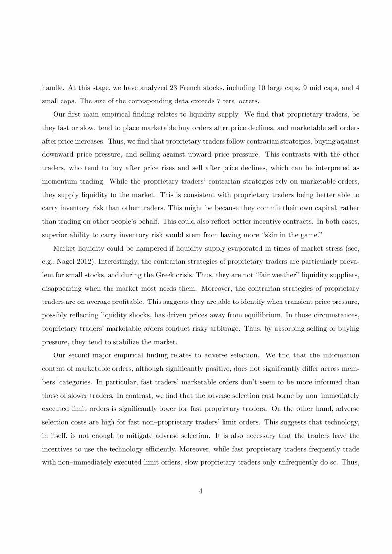
Our second major empirical finding relates to adverse selection. We find that the information

content of marketable orders, although significantly positive, does not significantly differ across mem-

bers’categories. In particular, fast traders’marketable orders don’t seem to be more informed than

those of slower traders. In contrast, we find that the adverse selection cost borne by non—immediately

executed limit orders is significantly lower for fast proprietary traders. On the other hand, adverse

selection costs are high for fast non—proprietary traders’limit orders. This suggests that technology,

in itself, is not enough to mitigate adverse selection. It is also necessary that the traders have the

incentives to use the technology effi ciently. Moreover, while fast proprietary traders frequently trade

with non—immediately executed limit orders, slow proprietary traders only unfrequently do so. Thus,

4

while slow proprietary traders mainly supply liquidity by placing contrarian marketable orders, fast

proprietary traders also supply liquidity by placing non immediately executed limit orders. We find,

however, that this second type of liquidity supply becomes much less prevalent after the crisis.

Literature: Our paper relates to the rich literature empirically analyzing algorithmic and high—

frequency trading:

Hendershott, Jones and Menkveld (2011) show that liquidity provision in equity market is provided

by algorithmic traders who are not offi cially designated as market makers.

Brogaard, Hendershott, Riordan (2014) analyze NASDAQ data, relying on a classification of

traders performed by the market organizers. They find that HFTs marketable orders have infor-

mation content, but not significantly more than other traders’marketable orders. They also find

that HFT’s orders tend to be contrarian and are on average profitable. Thus, our empirical findings

complement those of Brogaard, Hendershott, Riordan (2014) in two ways:

• Our findings relative to high—frequency traders are similar to theirs, and thus speak to the

robustness of their results to a different market and a different way to identify high—frequency

traders.

• Our findings on proprietary traders are new, and thus provide an incremental contribution to the

literature. We show that several characteristics of high-frequency traders’orders (i.e., contrarian,

profitable, and marketable) are also characteristics of the slow proprietary traders’orders in our

data. This suggests that these traders are able to place contrarian and profitable orders not

because they have low—latency, but because they are proprietary traders.5

Brogaard, Hagstromer, Norden, Riordan (2014) find that the choice to colocate is followed by

reduced adverse selection costs. Our results on adverse selection are in line with their findings. Our

incremental contribution, here, is to emphasize that technology may not be suffi cient to reduce adverse

selection. Appropriate incentives to use the technology effi ciently seem to be also needed.

Hendershott and Menkveld (2014) offer a state space model to identify how price pressure relates

to the specialist’s inventory. In a sense, the proprietary traders in our data play a similar role to the

5The high—frequency traders identified by NASDAQ are very likely to also be proprietary traders.

5

specialist in Hendershott and Menkveld (2014).6

Our paper is also in line with analyses of liquidity supply by market participants that are not

offi cially designated as market makers. Franzoni and Plazzi (2014) document liquidity supply by

hedge funds, classifying as liquidity supply purchases (resp. sales) at a price below (resp. above) a

benchmark (e.g., the opening price or the VWAP). Nagel (2012) argues that the returns on short—term

reversals can be interpreted as the returns from liquidity provision. Since, in our data, we observe

the type of the market participants and the details of their orders, we can rely on more precise data

to directly identify liquidity supply. Our empirical finding that proprietary traders supply liquidity

with profitable contrarian trades confirm the relevance of the approch of Nagel (2012) and Franzoni

and Plazzi (2014). Moreover, Nagel (2012) interprets high return on liquidity supply strategies when

the VIX is high as evidence that liquidity supply is reduced at those times. Our direct evidence on

liquidity supply offer some nuance on this point: On the one hand, we find that proprietary traders

continued to place profitable marketable contrarian orders during the Greek crisis of the summer of

2010, so, in that sense, liquidity did not “evaporate”. On the other hand, we find that the crisis

triggered a drop in the placement of non—immediately executed limit orders in small caps by fast

proprietary traders. Other things equal, this corresponds to a decline in liquidity supply.

The next section presents our data and summary statistics. Section 3 analyzes the placement and

informational content of marketable orders. Section 4 analyzes the adverse selection costs incurred

by non immediately executed limit orders. Section 5 summarizes our results and discusses policy

implications.

2 Market structure, data and summary statistics

Euronext is an electronic limit order market, operating continuously for most of the stocks. Orders

are submitted by the financial institutions that are members of Euronext. Members are assigned

an identification code. Most institutions have a single ID code, but some choose to have up to four

different codes to differentiate their activities (e.g., brokerage versus proprietary trading). Each ID

6Furthermore, Kirilenko, Kyle, Samadi, Tuzun (2014) find that HFTs did not cause the Flash Crash but exacerbated

it. Menkveld (2013) document liquidity supply by large HFT across ChiX & Euronext.

6

code can have several links to the exchange. The total fee charged by Euronext to a member depends

on the number of links connected to the Euronext servers, and on the capacity of each link. This

capacity is named “throughput”, and indicates the maximum number of messages (order submission,

cancellation or modification of an existing order) that the traders are allowed to send to the Exchange

in one calendar second via this link. The throughput of each link can be 10, 25, 50, 100, 200, 250,

or 500. It seems that a large throughput does not only increase the number of messages that can be

sent, but also increases the speed with which they reach the market. We are able to document this

empirically because, in our data, we observe (at the microsecond level) the time at which an order was

sent to the market and the time at which the order was executed. We also observe the throughput of

the link via which the order was sent. Marketable orders, by construction, are immediately executed.

Thus, for these orders, the difference between the execution time and the submission time is an inverse

measure of the speed of the connection. In Figure 1, panel A, we plot for each link, the median of

this time difference against the throughput of the link. The figure illustrates that links with higher

throughput tend to also have higher connection speed. Moreover, Euronext further proposes to its

Members to colocate their servers close to its owns.7 Colocation fees depend on the physical space

used by the Member, and on the electricity consumption of the servers.

We obtained our data from the Autorité des Marchés Financiers (the French financial markets

regulator) and Euronext. So far, we have analyzed 23 French stocks between February 2010 and

August 2010. The sample includes 10 large caps (1 financial and 9 non—financial with float between

1,048 and 3,884 million euros), 9 mid caps (1 financial and 8 non financial, with float between 181 and

960 million euros), and 4 small caps (all non financial, with float between 51 and 145 million euros).

150 Euronext member IDs traded these stocks during the sample period. 28 of them only traded

on their own account, and we classify them as prop traders. 37 only traded on behalf of customers and

we classify them as pure brokers. 85 conducted some trades on their own account and some trades on

behalf of customers. We classify them as dual traders.8

7 In May 2010, Euronext servers were moved to Basildon (in the neighbourhood of London, UK). Members can choose

to colocate some, all or none of their links.8Actually, for each trade we observe if it was reported by the member as proprietary or agency. But we have been told

by market participants that these reports can be quite noisy. To reduce the impact of such noise, we chose to classify as

pure proprietary traders those reporting only proprietary trades and as pure brokers those reporting only agency trades.

7

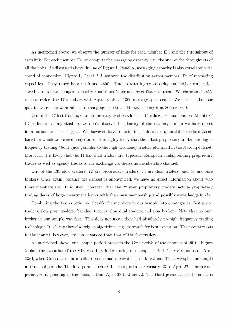
As mentioned above, we observe the number of links for each member ID, and the throughput of

each link. For each member ID, we compute the messaging capacity, i.e., the sum of the throughputs of

all the links. As discussed above, in line of Figure 1, Panel A, messaging capacity is also correlated with

speed of connection. Figure 1, Panel B, illustrates the distribution across member IDs of messaging

capacities. They range between 0 and 4600. Traders with higher capacity and higher connection

speed can observe changes in market conditions faster and react faster to them. We chose to classify

as fast traders the 17 members with capacity above 1300 messages per second. We checked that our

qualitative results were robust to changing the threshold, e.g., setting it at 800 or 1600.

Out of the 17 fast traders, 6 are proprietary traders while the 11 others are dual traders. Members’

ID codes are anonymized, so we don’t observe the identity of the traders, nor do we have direct

information about their types. We, however, have some indirect information, unrelated to the dataset,

based on which we formed conjectures. It is highly likely that the 6 fast proprietary traders are high—

frequency trading “boutiques”, similar to the high—frequency traders identified in the Nasdaq dataset.

Moreover, it is likely that the 11 fast dual traders are, typically, European banks, sending proprietary

trades as well as agency trades to the exchange via the same membership channel.

Out of the 133 slow traders, 22 are proprietary traders, 74 are dual traders, and 37 are pure

brokers. Once again, because the dataset is anonymized, we have no direct information about who

these members are. It is likely, however, that the 22 slow proprietary traders include proprietary

trading desks of large investment banks with their own membership and possibly some hedge funds.

Combining the two criteria, we classify the members in our sample into 5 categories: fast prop—

traders, slow prop—traders, fast dual traders, slow dual traders, and slow brokers. Note that no pure

broker in our sample was fast. This does not mean they had absolutely no high—frequency trading

technology. It is likely they also rely on algorithms, e.g., to search for best execution. Their connections

to the market, however, are less advanced than that of the fast traders.

As mentioned above, our sample period brackets the Greek crisis of the summer of 2010. Figure

2 plots the evolution of the VIX volatility index during our sample period. The Vix jumps on April

23rd, when Greece asks for a bailout, and remains elevated until late June. Thus, we split our sample

in three subperiods: The first period, before the crisis, is from February 23 to April 22. The second

period, corresponding to the crisis, is from April 23 to June 22. The third period, after the crisis, is

8

from June 23 to August 23.

Figure 3 depicts the number of trades per member, per stock, per day. Figure 3, Panel A, shows

that fast traders (both proprietary and dual) trade more often, and rely more on non immediately

executed limit orders, than slow traders. Slow proprietary traders trade less than fast traders, but more

than other slow traders. Moreover, unlike fast proprietary traders, they rely mainly on marketable

orders.

Panels B and C of Figure 3 show how these results vary with market capitalization and periods.

Comparing Panel B (large caps) and Panel C (small and mid caps), the number of trades is much

larger for the former than for the larger. Furthermore, for large caps the number of trades increases

during the crisis, but the relative frequencies of marketable orders and non—immediately executed limit

orders are rather stable through time. For small caps, however, the behavior of fast proprietary traders

is quite different. First their trading volume does not increase during the crisis. Second, while before

the crisis they frequently traded via non immediately executable limit orders, during and after the

crisis they considerably reduce their reliance on this type of trade. This is an important observation,

to which we come back below, when we analyze how the crisis affected adverse selection costs.

Figure 4 offers a graphical illustration of the frequency with which each category of traders’mar-

ketable orders hit each category of traders’ limit orders. Each color corresponds to the category of

the trader whose marketable order was executed. For example, the plain red bar corresponds to the

marketable orders placed by fast proprietary traders. It shows that, when a fast prop trader places

a marketable order, 19% of the time it hits another fast trader, 8% of the time it hits a slow prop

trader, 41% of the time it hits a fast dual trader, 27% of the time it hits a slow dual trader, and 4%

of the time it hits a pure broker’s order. Interestingly, the frequencies are very similar for marketable

orders placed by other categories of traders. So, it’s not the case that fast traders “target”a certain

category of trader’s limit orders.

3 Marketable orders

To estimate the information content of orders in the simplest possible way, we use the percentage

change from the midquote just before the trade to the midquote 2 minutes after the trade. Thus, for

9

a trade taking place at time t, the information content is

Mt+2 −Mt−

Mt−∗ signt,

where Mt− denotes the midquote just before the trade, Mt+2 denotes the midquote 2 minutes after

the trade, and signt takes the value 1 if the time—t marketable order is a buy order, and -1 if the

time—t marketable order is a sell order.

Figure 5, Panel A, depicts the informational content of the marketable orders placed by different

categories of traders. After a marketable buy (resp. sell) order placed by a fast proprietary trader,

the midquote increases (resp. decreases) on average by 3.5 basis points. The informational content

of the marketable orders placed by other categories of traders are not very different, ranging between

3.4 and 4.1 basis points. This suggests that the marketable orders placed by fast traders are not more

informed than the marketable orders placed by other traders. Correspondingly, they don’t generate

more adverse selection for limit orders standing in the book.

Figure 5, Panel B, depicts how the informational content of marketable orders varies across stocks

and through time.9 It shows that, for all traders, the informational content of orders is larger for small

caps and during the crisis, and remains higher after the crisis than before. Also, while, as shown in

Figure 5, Panel A, fast traders’orders are, in general, not better informed than other traders’orders,

during the crisis they are.

Figure 6 depicts the evolution of the midquote 5 minutes before and after the placement of a

marketable order by the different categories of traders, i.e., it plots the average of

Mt+h −Mt−

Mt−∗ signt,

where h varies from -5 minutes to +5 minutes. Panel A shows the results for large caps, while Panel

B shows the results for small caps. The two panels confirm the above discussed findings that, after

the trade, the information content of marketable orders is similar for all categories of members, and is

higher for small stocks. The new information in Figure 6, relative to Figure 5, is about what happens

before the trade. Figure 6 shows that dual traders or brokers place marketable buy (resp. sell) orders

9The information content of fast prop traders’orders is larger than that of other traders for all subcases in Panel

B. This does not contradict the fact that it is not higher in Panel A, because fast proprietary traders are relative more

active in large cap (for which the informational content of orders is lower) than in small caps.

10

after price increases (resp. decreases). This is consistent with dual traders and brokers riding short—

term momentum waves, or splitting orders. In stark contrast, fast proprietary traders (be they fast or

slow), buy after price decreases and sell after price increases. That is, they follow contrarian strategies.

Thus their marketable orders supply liquidity to the market, helping it accomodate buying or selling

pressure.

Is such liquidity supply robust ? Or does this liquidity evaporate when the market really needs it,

e.g., in times of crisis? To shed light on this, Figure 7 depicts the evolution of the midquote 5 minutes

before and after the placement of a marketable order, similarly to Figure 6, but distinguishing between

the period before the crisis (Panel A), during the crisis (Panel B) and after the crisis (Panel C). The

figure shows that there are no qualitative differences across periods. During the three periods, dual

traders and pure brokers buy after price rises and sell after price drops. And, during the three periods,

proprietary traders buy after price drops and sell after price rises. The only difference is that, during

the crisis, the magnitude of the price changes is larger. Thus, the liquidity supplied to the market by

the contrarian orders of proprietary traders does not seem to evaporate during times of market stress.

Our results are consistent with those of Brogaard, Hendershott, Riordan (2014), who find that

HFT’s marketable orders tend to be contrarian. Indeed, the HFT firms identified by Brogaard,

Hendershott, Riordan (2014) are likely to be proprietary traders. The new finding in the present

study is that slow traders also place such contrarian marketable orders, when they are proprietary

traders. This suggests that what enables traders to conduct such contrarian strategies is maybe not

technology but the ability to trade on one’s own account. That ability reduces agency conflicts between

investors and traders, and thus increases the ability to carry incentory, and, correspondingly, supply

liquidity to the market.

While such liquidity supply could be beneficial to the market, by accomodating liquidity shocks,

one could wonder whether it is sustainable. In particular, is it profitable? To shed light on this, we

computed the average profits of the marketable orders placed by the different categories of market

participants. To estimate the profitability of orders in the simplest possible way, we use the percentage

difference between the transaction price and the midquote 2 minutes after the trade. Thus, for a

marketable order executed at time t, the profit is

Mt+2 − PtMt−

∗ signt,

11

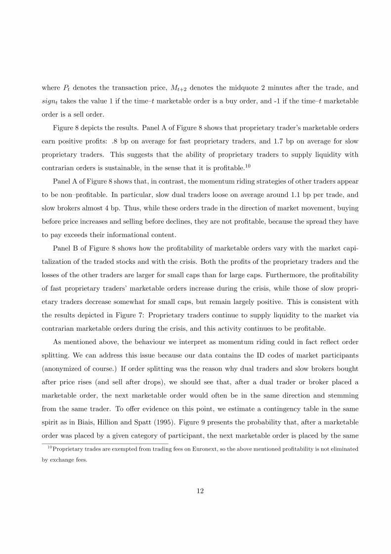
where Pt denotes the transaction price, Mt+2 denotes the midquote 2 minutes after the trade, and

signt takes the value 1 if the time—t marketable order is a buy order, and -1 if the time—t marketable

order is a sell order.

Figure 8 depicts the results. Panel A of Figure 8 shows that proprietary trader’s marketable orders

earn positive profits: .8 bp on average for fast proprietary traders, and 1.7 bp on average for slow

proprietary traders. This suggests that the ability of proprietary traders to supply liquidity with

contrarian orders is sustainable, in the sense that it is profitable.10

Panel A of Figure 8 shows that, in contrast, the momentum riding strategies of other traders appear

to be non—profitable. In particular, slow dual traders loose on average around 1.1 bp per trade, and

slow brokers almost 4 bp. Thus, while these orders trade in the direction of market movement, buying

before price increases and selling before declines, they are not profitable, because the spread they have

to pay exceeds their informational content.

Panel B of Figure 8 shows how the profitability of marketable orders vary with the market capi-

talization of the traded stocks and with the crisis. Both the profits of the proprietary traders and the

losses of the other traders are larger for small caps than for large caps. Furthermore, the profitability

of fast proprietary traders’marketable orders increase during the crisis, while those of slow propri-

etary traders decrease somewhat for small caps, but remain largely positive. This is consistent with

the results depicted in Figure 7: Proprietary traders continue to supply liquidity to the market via

contrarian marketable orders during the crisis, and this activity continues to be profitable.

As mentioned above, the behaviour we interpret as momentum riding could in fact reflect order

splitting. We can address this issue because our data contains the ID codes of market participants

(anonymized of course.) If order splitting was the reason why dual traders and slow brokers bought

after price rises (and sell after drops), we should see that, after a dual trader or broker placed a

marketable order, the next marketable order would often be in the same direction and stemming

from the same trader. To offer evidence on this point, we estimate a contingency table in the same

spirit as in Biais, Hillion and Spatt (1995). Figure 9 presents the probability that, after a marketable

order was placed by a given category of participant, the next marketable order is placed by the same

10Proprietary trades are exempted from trading fees on Euronext, so the above mentioned profitability is not eliminated

by exchange fees.

12

participant or another one, and is the same direction or the opposite one. The figure shows that,

after a marketable order was placed by a fast dual trader, the probability that the next marketable

order stems from the same trader is below 10%. For slow dual traders, this probability is between 10

and 15%, for slow brokers it is between 15 and 20%. These frequencies are not very large, suggesting

that order splitting is not the main driving force, and momentum trading is likely to be at play.

Interestingly, after a marketable order was placed by a fast prop trader, the probability that the next

marketable order stems from the same trader is very low (around 5%), while after a marketable order

from a slow prop trader its is very large (above 35%). This suggests, that, at least in the case of slow

prop traders, order splitting and contrarian liquidity supply coexist. Another implication from Figure

9 is that order splitting seems to be more prevalent for slow traders than for fast traders.

The overall message emerging from the above discussed findings is the following: Slow traders tend

to split orders, while fast traders engage less in order splitting. Proprietary traders help the market

absorb liquidity shocks by placing contrarian marketable orders, while other traders tend to consume

liquidity by riding momentum waves.

4 Adverse selection costs incurred by limit orders

Limit orders left in the book are exposed to adverse selection, as analyzed, e.g., by Glosten and

Milgrom (1985), Glosten (1994) and Biais, Martimort and Rochet (2000). Fast trading technology,

however, enhances traders’ability to monitor market movements. This may enable them to cancel or

modify stale quotes, before they receive adverse execution.

To estimate the adverse selection cost incurred by limit orders in the book, we use the percentage

change from the midquote just before the trade to the midquote 2 minutes after the trade. Thus, for

a trade taking place at time t, the information content is

Mt+2 −Mt−

Mt−∗ signlimitt ,

where Mt− denotes the midquote just before the trade, Mt+2 denotes the midquote 2 minutes after

the trade, and signlimitt takes the value 1 if the limit order hit at time—t is a buy order, and -1 if it is

a sell order. This is similar to the measure of information content illustrated in Figure 5, but, while

in Figure 5 we condition on the type and direction of the aggressive marketable order, in Figure 10

13

we condition on the type and direction of the passive limit order (hit by a marketable order).

Figure 10, Panel A, shows that, after a limit buy (resp. sell) order left in the book by a fast

proprietary trader is executed, the midquote decreases (resp. increases) on average by 2.8 basis

points. The adverse selection costs of limit orders left in the book by other categories of traders are

3.1 bp for slow proprietary traders, 3.8 bp for fast dual traders, 4.1 bp for slow dual traders and 5

bp for slow brokers. Thus, the adverse selection cost is lowest for fast proprietary traders. Adverse

selection costs are higher for fast non—proprietary traders. This suggests that technology, in itself, is

not enough to mitigate adverse selection. It is also necessary that the traders have the incentives to

use the technology effi ciently.

Figure 10, Panel B, compares adverse selection costs before, during and after the crisis, and also

across large and small caps. Overall, adverse selection costs are higher for small caps. They are also

higher during the crisis. There are some differences between the different categories of traders:

• For non—proprietary traders, adverse selection costs increase during the crisis, and remain ele-

vated afterwards.

• For slow proprietary traders, there is a similar pattern, except that adverse selection costs decline

after the crisis.

• For fast proprietary traders, while the pattern is similar for small and mid caps, for large caps

adverse selection costs remain low throughout the period, and are not higher during or after

the crisis. This is consistent with the patterns depicted in Panels B and C of Figure 3: Fast

proprietary traders seem to be able to control adverse selection costs for large caps during the

crisis, and thus continue to supply liquidity in these stocks via limit orders. In contrast, for small

and mid caps, their adverse selection costs increase and they reduce their limit order liquidity

supply. This is a form of “liquidity evaporation.”

Figure 11 depicts the profits earned by limit orders left in the book, estimated as

Mt+2 − PtMt−

∗ signlimitt ,

where Pt denotes the transaction price, Mt+2 denotes the midquote 2 minutes after the trade, and

signlimitt takes the value 1 if the limit order hit at time—t is a buy order, and -1 if it is a sell order.

14

Panel A of Figure 11 shows that the limit orders of fast proprietary traders (and also those of slow

dual traders) earn slightly positive profits on average. That is, for these orders, the bid—ask spread

(which they earn) is slightly larger than the adverse selection cost (which they incur). In contrast,

the limit orders left in the book by dual fast traders loose 3 bp per trade on average, and those of

slow proprietary traders 8 bp per trade. That is, for these limit orders the adverse selection cost is so

large that it exceeds the spread. This is consistent with i) our observation above that slow proprietary

traders rarely use non—immediately executable orders and ii) the conjecture that they are aware that

such orders would be loss making for them.

Panel B of Figure 11 shows that the profitability of non immediately executed limit orders varies

considerably with capitalization and period. Both losses and profits are much lower for large caps.

The most striking result is the large profitability of fast proprietary traders’ limit orders in small

caps during the crisis and afterwards. These are the most diffi cult stocks and times, for which adverse

selection costs are the largest, as shown in Figurer 10, Panel B. Yet, fast proprietary traders apparently

are able to earn the spread to such an extent that they more than offset these costs.

The results in Figures 10 and 11 suggest that fast proprietary traders’limit orders are less adversely

selected than others, in line with the notion that fast proprietary traders monitor the market and often

cancel or modify their orders before receiving adverse execution. To document this point, we computed

the number of cancellations and the number of updates to less aggressive quotes for each category of

trader, normalizing these numbers by the number of trades. Figure 12 shows that, for fast proprietary

traders, the number of updates to less aggressive quotes is 3.7 times as large as the number of trades

outside the crisis, and 4.2 times during the crisis. For cancellations, these numbers are 12.8 outside

the crisis, and 15.1 during the crisis. These numbers are much larger than the corresponding numbers

for fast dual traders and much, much larger than the corresponding numbers for other categories of

traders. That the frequency of cancellations and modifications by fast proprietary traders is higher

during the crisis, suggests that these traders exerted more effort monitoring the market and adjusting

to it. The cost of this effort increased the cost of leaving limit orders in the book during the crisis.

15

5 Conclusion and policy implications

We analyze a unique dataset enabling us to observe, in addition to time stamped orders and trades

on Euronext, the number of messages per second traders can exchange with the market, and whether

they are prop traders. Our sample period, in 2010, brackets the Greek crisis of the summer of 2010.

We find that proprietary traders, be they fast or slow, tend to place marketable buy orders af-

ter price drops, and marketable sell orders after price increases. And, after they have bought, the

market tends to recover, while, after they have sold, the market tends to retreat. This is consistent

with proprietary traders helping the market accomodate liquidity shocks, and thus reducing transient

deviation from effi cient pricing. Moreover, we find that this liquidity supply remains available during

the crisis. In that sense, liquidity supply by proprietary traders does not evaporate when it is most

needed.

We also find that the limit orders of fast proprietary traders (but not other fast traders) incur lower

adverse selection costs than the limit orders of other traders. Our results suggest that fast proprietary

traders supply liquidity to the market via contrarian marketable orders and non—immediately executed

limit orders, while slow proprietary traders supply liquidity only via contrarian marketable orders. The

crisis, however, triggered a decline the in the placement of non—immediately executable for small and

mid caps by fast proprietary traders. In that sense, some liquidity “evaporated.”

Our empirical findings suggest that current regulatory reforms might have unintended negative

consequences:

• Under MIFID 2, trading venues will be required to cap the ratio of the number of messages to

the number of trades by participant. This might be counterproductive, as our findings suggest

that fast proprietary traders rely on numerous cancellations and updates to reduce the adverse

selection cost incurred by their limit orders. Capping the percentage of cancellations and updates

could increase the adverse selection costs incurred by limit orders left in the book, and thus deter

the provision of liquidity by these orders. This could be harmful for market liquidity, especially

at times of market stresss, when the need to modify and cancel orders is particularly acute.

• In this context, new banking regulations, making it more diffi cult and costly for banks to engage

in proprietary trading, might also reduce market liquidity.

16

References

Biais, B., J. Hombert and P. O. Weill, 2014, “Equilibrium Pricing and Trading Volume under

Preference Uncertainty,”Review of Economic Studies.

Biais, B., P. Hillion, and C. Spatt, 1995, “An Empirical Analysis of the Limit Order Book and the

Order Flow in the Paris Bourse,”Journal of Finance, 50, 1655-1689.

Biais, B., D. Martimort, and J. Rochet, 2000, “Competing Mechanisms in a Common Value

Environment,”Econometrica, 68, 799-838.

Brogaard, J., T. Hendershott and R. Riordan, 2014, “High-Frequency Trading and Price Discov-

ery,”Review of Financial Studies, 27, 2267-2306.

Brogaard, J., B. Hagströmer, L. Nordén, and R. Riordan, 2014, “Trading fast and slow: colocation

and market quality,”Working paper, University of Stockholm.

Franzoni, F. and A. Plazzi, 2014, “What constrains liquidity provision? Evidence from hedge fund

trades.”Working paper, Swiss Finance Institute.

Glosten, L., 1994, “Is the Electronic Open Limit Order Book Inevitable?”Journal of Finance, 49,

1127-1161.

Glosten, L., and P. Milgrom, 1985, “Bid, Ask and Transaction Prices in a Specialist Market with

Heterogeneously Informed Traders,”Journal of Financial Economics, 14, 71-100.

Gromb, D. and D. Vayanos, 2010, “Limits of Arbitrage: The State of the Theory”, NBER Working

paper No. 15821.

Gromb, D. and D. Vayanos, 2002, “Equilibrium and Welfare in Markets with Financially Con-

strained Arbitrageurs,”Journal of Financial Economics 66, 361-407.

Gromb, D. and D. Vayanos, 2015, “The Dynamics of Financially Constrained Arbitrage”, Working

paper, LSE.

Grossman, S., and M. Miller, 1987, “Liquidity and market structure,”Journal of Finance, 617—633.

Hendershott, T., C. Jones and A. Menkveld, 2011, “Does algorithmic trading improve liquidity?”

Journal of Finance, 66, 1—33.

Ho, T., and H. Stoll, 1983, “The Dynamics of Dealer Markets Under Competition,” Journal of

Finance, 38, 1053-1074.

17

Ho, T., and H. Stoll, 1981, “Optimal Dealer Pricing Under Transactions and Return Uncertainty,”

Journal of Financial Economics, 9, 47-73.

Nagel, S., 2012, “Evaporating Liquidity,”Review of Financial Studies, 25, 2005—2039.

Shleifer, A., and R. Vishny, 1997, “The limits of arbitrage,”Journal of Finance, 52, 37—55.

Weill, P.O., 2007, “Leaning against the Wind,”Review of Economic Studies, 74, 1329—1354.

18

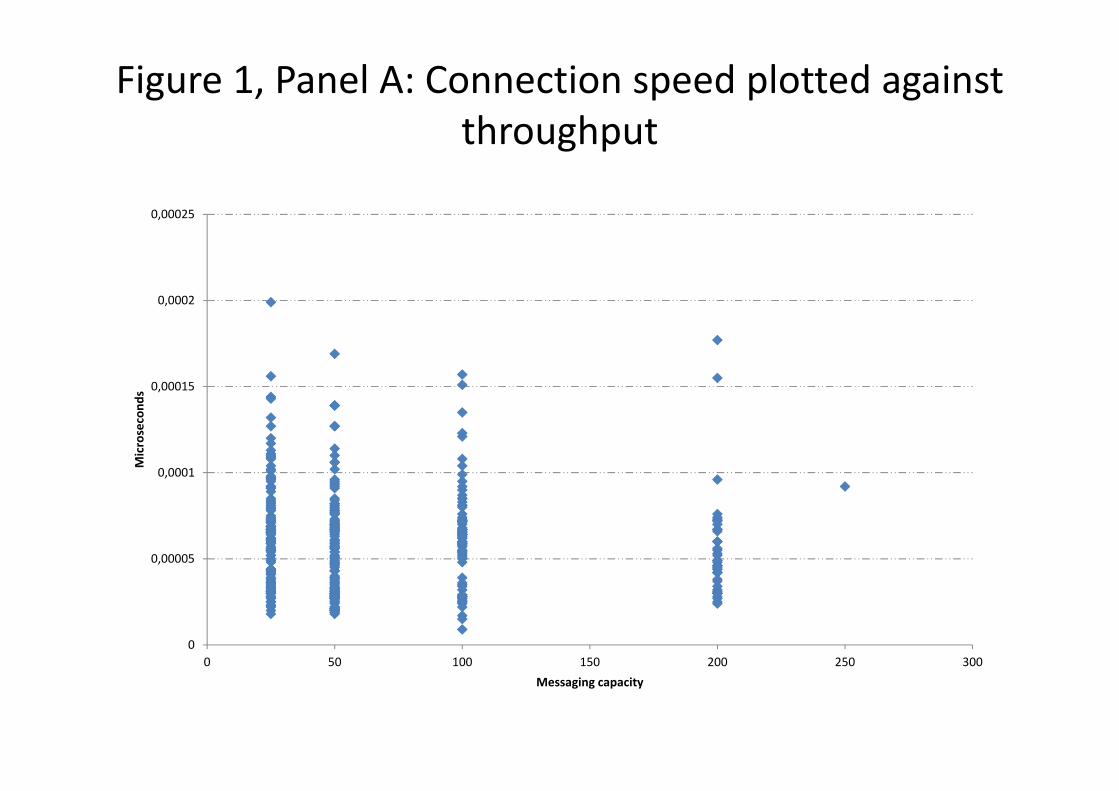
Figure 1, Panel A: Connection speed plotted againstthroughput

0

0,00005

0,0001

0,00015

0,0002

0,00025

0 50 100 150 200 250 300

Microsecond

s

Messaging capacity

0%

2%

4%

6%

8%

10%

12%

14%

16%

18%

[0 - 25] ]25 - 50] ]50 - 75] ]75 -100]

]100 -150]

]150 -200]

]200 -300]

]300 -400]

]400 -800]

]800 -1300]

]1300 -1600]

]1600 -2400]

]2400 -4600]

% of members

Max # messages per second

Figure 1, Panel B: Distribution of trading capacity across members

0

5

10

15

20

25

30

35

40

45

50

Jan-10 Feb-10 Mar-10 Apr-10 May-10 Jun-10 Jul-10 Aug-10 Sep-10

VIX

CrisisModeratevolat

April 23: Grece asks for bailout

May 7: June 14:  bailout downgrade

Low volat

Figure 2: VIX during the sample period

Figure 3, Panel A: Number of trades per member, stock and day

0

10

20

30

40

50

60

70

fast prop slow prop fast dual slow dual slow brokers

limit marketable

Figure 3, Panel B: Number of trades per member, stock and day – Large caps by period

0

20

40

60

80

100

120

140

160

fast prop slow prop fast dual slow dual slow brokers

Large caps, pre‐crisis limit Large caps, pre‐crisis marketable Large caps, crisis limit Large caps, crisis marketable Large caps, post‐crisis limit Large caps, post‐crisis marketable

Figure 3, Panel C: Number of trades per member, stock and day – Small and mid caps by period

0

5

10

15

20

25

fast prop slow prop fast dual slow dual slow brokers

Small & mid  caps, pre‐crisis limit Small & mid  caps, pre‐crisis marketable Small & mid  caps, crisis limit

Small & mid  caps, crisis marketable Small & mid  caps, post‐crisis limit Small & mid  caps, post‐crisis marketable

0%

5%

10%

15%

20%

25%

30%

35%

40%

45%

50%

Fast prop (888432obs)

Slow prop (377028obs)

Fast dual (1929653obs)

Slow dual 1276199obs)

Slow broker (167523obs)

Fast prop

Slow prop

Fast dual

Slow dual

Slow brokers

Figure 4: Who trades with whom?

Who placedthe marketableorder

Who placed the limit order that got hit

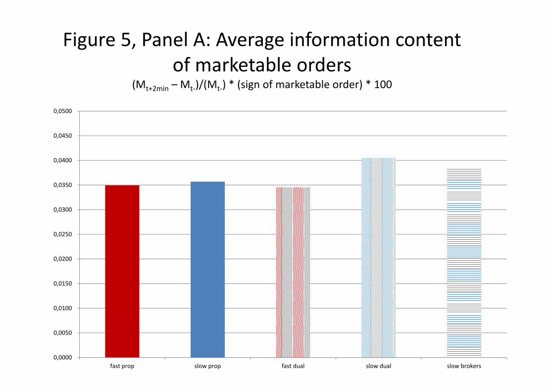
Figure 5, Panel A: Average information content of marketable orders

(Mt+2min – Mt‐)/(Mt‐) * (sign of marketable order) * 100

0,0000

0,0050

0,0100

0,0150

0,0200

0,0250

0,0300

0,0350

0,0400

0,0450

0,0500

fast prop slow prop fast dual slow dual slow brokers

Figure 5, Panel B: How does the information content of marketable orders vary?

(Mt+2min – Mt‐)/(Mt‐) * (sign of marketable order) * 100

0,0000

0,0100

0,0200

0,0300

0,0400

0,0500

0,0600

0,0700

0,0800

0,0900

0,1000

Pre‐crisis Crisis Post‐crisis Pre‐crisis Crisis Post‐crisis

 small & mid caps  large caps

fast prop

slow prop

fast dual

slow dual

slow brokers

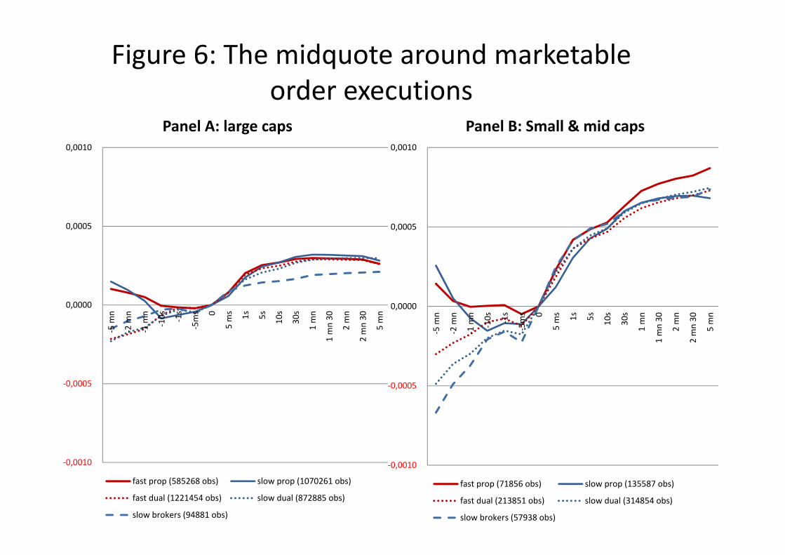
Figure 6: The midquote around marketableorder executions

‐0,0010

‐0,0005

0,0000

0,0005

0,0010

 ‐5 m

n

 ‐2 m

n

 ‐1 m

n

 ‐10s  ‐1s

 ‐5ms 0

5 ms 1s 5s 10s

30s

1 mn

1 mn 30

2 mn

2 mn 30

5 mn

Panel A: large caps

fast prop (585268 obs) slow prop (1070261 obs)

fast dual (1221454 obs) slow dual (872885 obs)

slow brokers (94881 obs)

‐0,0010

‐0,0005

0,0000

0,0005

0,0010

 ‐5 m

n

 ‐2 m

n

 ‐1 m

n

 ‐10s  ‐1s

 ‐5ms 0

5 ms 1s 5s 10s

30s

1 mn

1 mn 30

2 mn

2 mn 30

5 mn

Panel B: Small & mid caps

fast prop (71856 obs) slow prop (135587 obs)

fast dual (213851 obs) slow dual (314854 obs)

slow brokers (57938 obs)

Figure 7: Momentum and contrarianmarketable orders during crisis

‐0,0010

‐0,0005

0,0000

0,0005

0,0010

 ‐5 m

n

 ‐1 m

n

 ‐1s 0 1s 10s

1 mn

2 mn

5 mn

Panel A: Pre‐crisis

‐0,0010

‐0,0005

0,0000

0,0005

0,0010

 ‐5 m

n

 ‐1 m

n

 ‐1s 0 1s 10s

1 mn

2 mn

5 mn

Panel B: Crisis

‐0,0010

‐0,0005

0,0000

0,0005

0,0010

 ‐5 m

n

 ‐1 m

n

 ‐1s 0 1s 10s

1 mn

2 mn

5 mn

Panel C: Post‐crisis

Figure 8, Panel A: Marketable orders’ profits(Mt+2min – Pt)/(Mt‐) * (sign of marketable order) * 100

‐0,0400

‐0,0300

‐0,0200

‐0,0100

0,0000

0,0100

0,0200

fast prop slow prop fast dual slow dual slow brokers

‐0,0010

‐0,0008

‐0,0006

‐0,0004

‐0,0002

0,0000

0,0002

0,0004

0,0006Pre‐crisis Crisis Post‐crisis Pre‐crisis Crisis Post‐crisis

 small & mid caps  large caps

fast prop

slow prop

fast dual

slow dual

slow brokers

Figure 8, Panel B: Marketable orders’ profits by periods and by capitalization

Figure 9: Prob(marketable order n|marketable order n‐1)

0%

5%

10%

15%

20%

25%

30%

35%

40%

fast prop slow prop fast dual slow dual slow broker

marketable order at date t‐1

same trader, same direction

same trader, opp. direction

fast prop, same direction

fast prop, opp. Direction

slow prop, same direction

slow prop, opp. Direction

fast dual, same direction

fast dual, opp. Direction

slow dual, same direction

slow dual, opp. Direction

slow broker, same direction

slow broker, opp. Direction

Figure 10,panel A: Adverse selection cost for (non immediately executed) limit orders

(Mt+2min – Mt‐)/(Mt‐) * (sign of limit order) *100

‐0,0500

‐0,0450

‐0,0400

‐0,0350

‐0,0300

‐0,0250

‐0,0200

‐0,0150

‐0,0100

‐0,0050

0,0000fast prop slow prop fast dual slow dual slow brokers

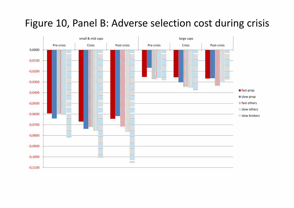
Figure 10, Panel B: Adverse selection cost during crisis

‐0,1100

‐0,1000

‐0,0900

‐0,0800

‐0,0700

‐0,0600

‐0,0500

‐0,0400

‐0,0300

‐0,0200

‐0,0100

0,0000Pre‐crisis Crisis Post‐crisis Pre‐crisis Crisis Post‐crisis

 small & mid caps  large caps

fast prop

slow prop

fast others

slow others

slow brokers

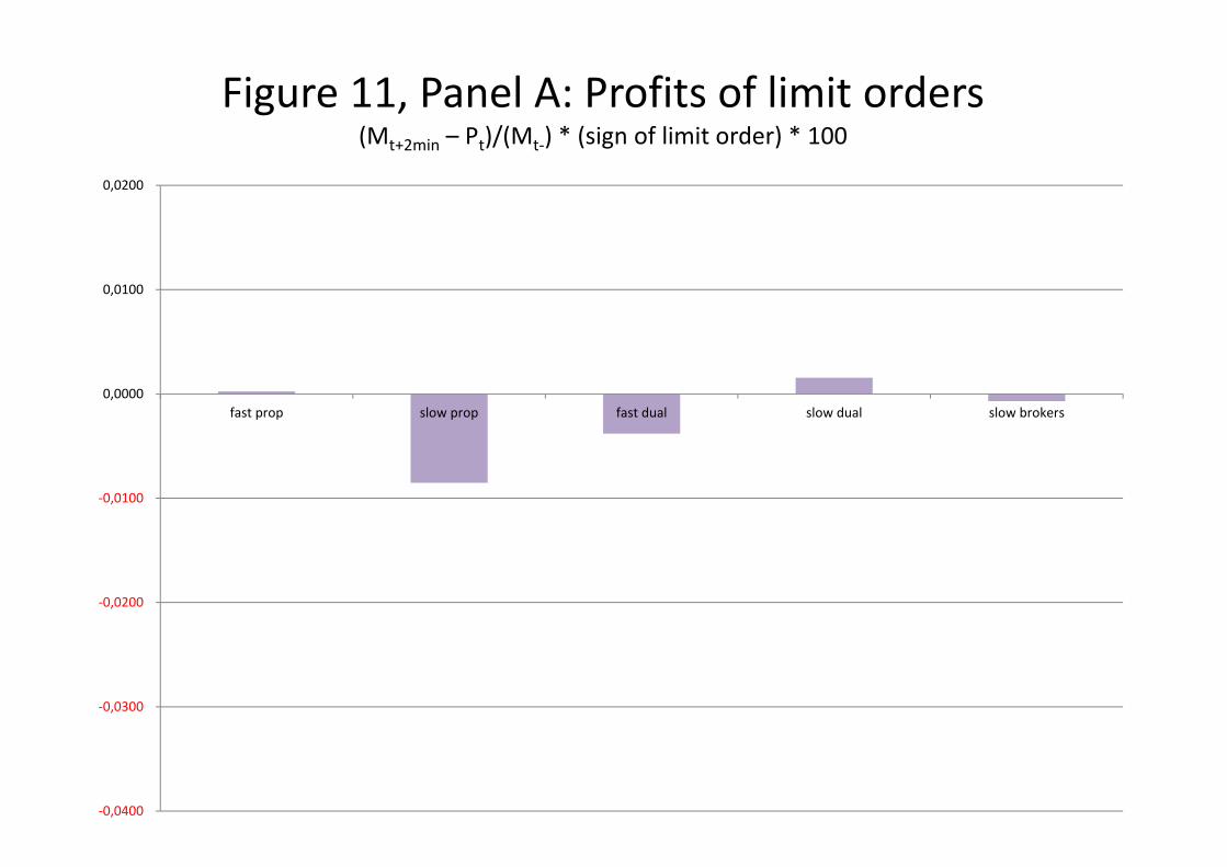
Figure 11, Panel A: Profits of limit orders(Mt+2min – Pt)/(Mt‐) * (sign of limit order) * 100

‐0,0400

‐0,0300

‐0,0200

‐0,0100

0,0000

0,0100

0,0200

fast prop slow prop fast dual slow dual slow brokers

‐0,0002

‐0,0001

0,0000

0,0001

0,0002

0,0003

0,0004

Pre‐crisis Crisis Post‐crisis Pre‐crisis Crisis Post‐crisis

 small & mid caps  large caps

fast prop

slow prop

fast dual

slow dual

slow brokers

Figure 11, Panel B: Profits of limit orders by capitalization and period

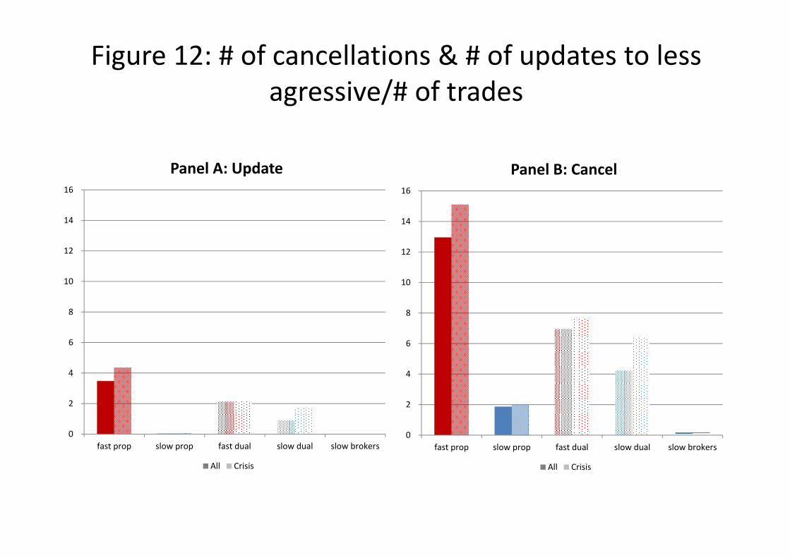
Figure 12: # of cancellations & # of updates to lessagressive/# of trades

0

2

4

6

8

10

12

14

16

fast prop slow prop fast dual slow dual slow brokers

Panel B: Cancel

All Crisis

0

2

4

6

8

10

12

14

16

fast prop slow prop fast dual slow dual slow brokers

Panel A: Update

All Crisis