Who Method for Life Table

8/3/2019 Who Method for Life Table

http://slidepdf.com/reader/full/who-method-for-life-table 1/33

1

WHO System of Model Life Tables

C.J.L. MurrayO.B. AhmadA.D. Lopez

J.A. Salomon

GPE Discussion Paper Series: No. 8

EIP/GPE/EBDWorld Health Organization



2

Introduction

The life table provides the most complete description of mortality in any population. The basic

data input needed for its construction are the age-specific death rates calculated from information

on deaths by age and sex (from vital registration) and population by age and sex (from census).

In many developing countries, these basic data either do not exist due to lack of functioning vital

registration systems, or are unusable because of incompleteness of coverage or errors in

reporting. Where the issue is principally one of incompleteness, demographers have devised

ingenious ways of deriving reasonably suitable life tables after the application of a variety of

appropriate adjustment techniques. In cases of unusable or non-existent vital registration data,

indirect techniques for obtaining mortality rates are employed. These techniques are predicated

on the observed similarities in the age-patterns of mortality for different populations, and may

range from the simple adoption of the mortality pattern of a neighbouring population with similar socio-biological characteristics, to the use of sophisticated demographic models.

The observed regularities in the age pattern of mortality is the prime motivation in the search for

mathematical functions that fully capture the observed variations of mortality with age

(Gompertz, 1825; Keyfitz, 1984). Failure to achieve this has led to the development of a number

of empirical “universal” mortality models (or model life tables) of varying degrees of

sophistication. The best known are (i) the UN Model Life Tables, (ii) The Coale-Demeny Model

Life Tables, (iii) the UN Model Life Tables for Developing countries, (iv) the Ledermann

System of Model Life Tables and (v) the Brass Logit System. The data underlying them vary in

the range of human experience they encompass. As such, particular mortality models may be

more or less suitable for specific geographic areas.

These models have contributed significantly to our understanding of levels and patterns of

mortality over the last half century in areas of the world with very little demographic data. There

are, however, substantial drawbacks to their continued use in many contemporary developing

countries. Principally, the restricted nature of the original sample of life tables that underlie these

models has always been a major disadvantage. It has become more so with the spread of

HIV/AIDS whose effect on the age pattern of mortality has no corollary in recent history.

Linked to these are the likely differences between the historical cause of death structure

underlying these models and the cause of death structure prevailing in many developing

countries today. Also, several of the models are essentially uni-parametric and therefore

relatively inflexible. In this regard, the Brass logit system offers considerable advantages by

being essentially independent of historical data. Such flexibility could be harnessed in extending

its application to situations of extreme data poverty, e.g. in Africa and parts of SE Asia. The

present paper presents a candidate method for achieving this, based on the relationship between



3

under-five mortality (5q0) and adult mortality (45q15) within a space bounded by the parameters of

the logit system. The technique allows the derivation of complete life tables from a knowledge

of the under-five mortality, the adult mortality (45q15) and a corresponding WHO regional

standard life table. It forms the basis for a new WHO system of model life tables.

In the subsequent sections, we provide a historical perspective on the development, shortcomings

and relative advantages of the model life table systems currently available. We assess, in

particular, the performance of the Coale Demeny model life table system relative to the logit. We

then rigorously evaluate and quantify the biases inherent in these models using both real data and

hypothetical data from the four families of the Coale-Demeny model life tables. We finally

evaluate the performance of the WHO system against real data. Detailed derivations of formulae

are shown in the appendix.

Historical perspectives

The basic objective in the creation of any model life table is to construct a system that gives

schedules of mortality by sex and age, defined by a small number of parameters that capture the

level as well as the age pattern of mortality. If a particular model adequately represents reality,

the characteristics of a given population can be summarized by the parameters of that model,

thereby facilitating the study of variation among populations or within a population over time.Thus, model life tables are essential demographic tools for populations lacking accurate

demographic data. The principles underlying each of the existing model life tables are discussed

below.

UN model life tables (1955). The first set of model life tables was published by the UN in 1955.

They were constructed using 158 life tables for each sex, using statistical techniques to relate

mortality at one age to mortality at another age for a range of mortality levels. The model

assumes that the value of n q

xfor each age interval in a life table is a quadratic function of the

rate in the preceding interval, namely 5 qx-n (except for the first two age groups, 1q0 and 4q1, all

the other groups considered are 5 years in length). Thus, knowledge of only one mortality

parameter (e.g., 1q0 or equivalently the mortality level that indexes the 1q0 values used)

determines a complete life table. For this reason, the UN model life tables are collectively

referred to as a one-parameter system. To each level of mortality there corresponds a model life

table for males, females and both sexes combined.

The coefficients of the quadratic equations for each sex were estimated from the corresponding

sample of 158 life tables. These were then used in generating the actual model life tables by first



4

choosing, arbitrarily, a convenient value of 1q0. This value was then substituted in the equation

relating 1q0 to 1q4 in order to obtain a value for 1q4, which in turn was substituted in the equation

relating 5q5 to 1q4 to obtain 5q5 , etc., etc. This “chaining” process continued until the model life

table was completed.

The Coale and Demeny regional model life tables. These were first published in 1966. They were

derived from a set of 192 life tables, by sex, from actual populations. This set included life tables

from several time periods (39 from before 1900 and 69 from after the Second World War) and

mostly from Western countries. Europe, North America, Australia and New Zealand contributed

a total of 176 tables. Three were from Israel; 6 from Japan, 3 from Taiwan; and 4 from the white

population of South Africa. All of the 192 selected life tables were derived from registration

data, and were subjected to very stringent standards of accuracy.

Further analysis of the underlying relationships identified four typical age patterns of mortality,

determined largely by the geographical location of the population, but also on the basis of their

patterns of deviations from previously estimated regression equations. Those patterns were

called: North, South, East, and West. Each had a characteristic pattern of child mortality. The

East model comes mainly from the Eastern European countries, and is characterized by high

child mortality in relation to infant mortality. The North model is based largely on the Nordic

countries, and is characterized by comparatively low infant mortality, high child mortality and

low old age mortality beyond age 50. The South model is based on life tables from the countriesof Southern Europe (Spain, Portugal, and southern Italy), and has a mortality pattern

characterized by (a) high child mortality in relation to infant mortality at high overall mortality,

and (b) low child relative to infant mortality at low overall mortality. The West model is based on

the residual tables not used in the other regional sets (i.e., countries of Western Europe and most

of the non-European populations). It is characterized by a pattern intermediate between North

and the East patterns. Because this model is derived from the largest number and broadest

variety of cases, it is believed to represent the most general mortality pattern. In this system, any

survivorship probability, whether from birth or conditional on having attained a certain age,

uniquely determines a life table, once a family has been selected. Although technically a one

parameter system, it could be argued that the choice of a family constitutes a separate dimension.

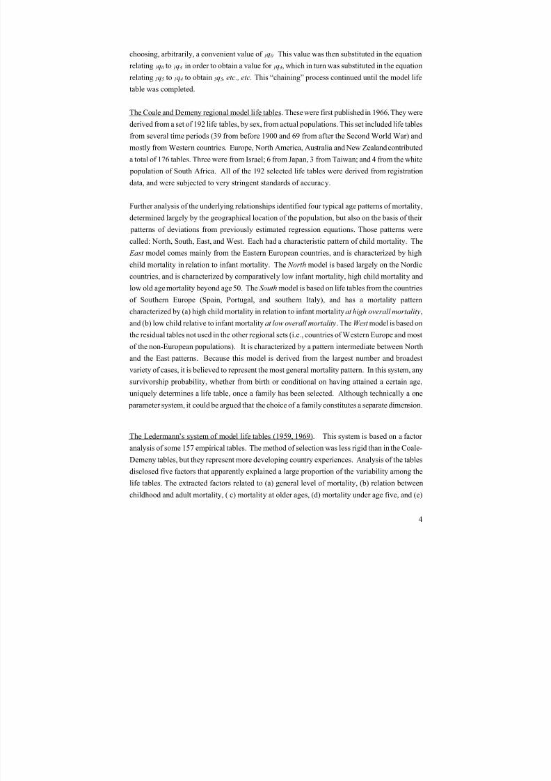
The Ledermann’s system of model life tables (1959, 1969). This system is based on a factor

analysis of some 157 empirical tables. The method of selection was less rigid than in the Coale-

Demeny tables, but they represent more developing country experiences. Analysis of the tables

disclosed five factors that apparently explained a large proportion of the variability among the

life tables. The extracted factors related to (a) general level of mortality, (b) relation between

childhood and adult mortality, ( c) mortality at older ages, (d) mortality under age five, and (e)



5

male-female difference in mortality in the age range 5-70 years. Later, Ledermann developed a

series of one- and two-parameter model life tables based on these result i.

Brass logit system (1971). This system provides a greater degree of flexibility than the empirical

models discussed above. It rests on the assumption that two distinct age-patterns of mortality can

be related to each other by a linear transformation of the logit of their respective survivorship

probabilities. Thus for any two observed series of survivorship values, l x and l s x , where the latter

is the standard, it is possible to find constants a and b such that

for all age x between 1 and T . If the above equation holds for every pair of life tables, then any

life table can be generated from a single standard life table by changing the pairs of (" ,$ ) values

used. In reality, the assumption of linearity is only approximately satisfied by pairs of actual life

tables. However, the approximation is close enough to warrant the use of the model to study and

fit observed mortality schedules. The parameter " varies the mortality level of the standard,

while $ varies the slope of the standard, i.e., it governs the relationship between the mortality in

children and adults. Figure 1 shows the result of varying " and $ . As $ decreases, there is higher

survival in the older ages relative to the standard, and vice versa. Higher values of " at a fixed $

lead to lower survival relative to the standard.

The UN model life table for developing countries (1981). These were designed to address the

needs of developing countries. The underlying data consisted of 36 life tables covering a wide

range of mortality levels from developing countries, by sex. Sixteen pairs of life tables came

from 10 countries in Latin America, 19 pairs from 11 countries in Asia, and one pair from Africa.

Five families of models were identified, each with a set of tables ranging from a life expectancy

of 35 to 75 years for each sex. Each family of models covers a geographical area: Latin

American, Chilean, South Asian, Far Eastern and a General . The general model was

constructed as an average of all the observations.

( ) ( )

( )

logit l

logit l

Then

x

x

= +

=-æ

è çö

ø÷

-æ

è ç

ö

ø÷ = +

-æ

è ç

ö

ø÷

a b

a b

log

. ln ( . )

. ln( . )

. ln( .

it l

if l l

l

l

l

l

x

s

x

x

x

x

x

s

x

s

0 5 10

0 510

0 510



6

Shortcomings of the empirical MLTs

There are three major criticisms of the UN model life tables. First, the fact that they are one-

parameter systems makes them relatively inflexible. Such a single parameter model cannot

adequately describe the complex mortality patterns available. In some cases, they have failed todescribe adequately life tables that were known to be accurate (Menken, 1977). Second, because

the estimate of mortality in each age-group is ultimately linked to the infant mortality rate

through the chaining process, measurement errors are easily accentuated. The third criticism

concerns the poverty of developing country life tables in the original design of the model.

Additionally, some of the empirical tables included were of dubious quality (UN, 1983). The

UN model life tables for developing countries also suffer from some of these limitations. Hence,

both systems of UN model life tables have a selective if not a limited range of application.

The Coale-Demeny model life tables had much higher standards of accuracy for the empirical

tables. This demand, however, limited the number of non-European countries represented. As

such, the Coale-Demeny tables may not cover patterns of mortality existing in the contemporary

developing world. In fact, there are examples of well documented mortality patterns that lie

outside the range of the Coale-Demeny tables. In particular, Demeny and Shorter found no table

within the family that adequately refleceted the Turkish mortality experience (Demeny &

Shorter, 1968). Although the North, South, East and West classification provides an added

dimension, the uni-parametric nature of each family still limits its flexibility.

The Ledermann system is criticized primarily for its relative complexity which essentially

precludes its use in most developing countries. Even though it does provide some flexibility

through a wider variety of entry values, in practice most of these values are not easily estimated

for most developing countries. This drawback reduces its relative advantages over the UN and

the Coale-Demeny models. A second major limitation is that the independent variables used in

deriving the model refer, with only one exception, to parameters obtained from data on both

sexes combined. The user is, therefore, forced to accept the relationships between male and

female mortality embodied in the model even when there is evidence to the contrary. For

instance, it is near impossible to estimate a Ledermann model life table in which the male

expectation of life exceeds that of females (UN, 1977).

Another shortcoming common to all three empirical models is their dependence on the type of

data that generated them. The databases upon which they were built exclude a significant

proportion of possible mortality schedules. Although the UN set of model life tables attempted



7

to address this issue, there were serious flaws in the selection of life tables as well as the criteria

of acceptance.

It is clear, therefore, that there are serious technical issues that complicate the use of existing

empirical models in describing mortality patterns in contemporary developing countries. These

are further compounded by the emergence of HIV/AIDS as a major cause of death in Africa and

parts of Asia. For these and other reasons WHO is proposing a new three-parameter system of

model life tables anchored on the logit system. The choice of the logit system was based on a

careful comparative evaluation of the logit and the Coale-Demeny systems. This evaluation

process is presented in the next section.

Contrasting the logit with the Coale -Demeny MLTs

Since the Coale-Demeny is the most extensively used of the empirical models, discussions will

be limited to it and the logit system. In contrast to the Coale-Demeny models, the logit system is

not dependent on any fixed empirical data. It allows the choice of a locally-applicable standard

life table. Once a suitable standard life table or equivalently a standard series of l x values has

been selected, the problem reduces to finding appropriate set of values of " and $ . A life table

can then be generated using the logit equations presented earlier. It is, therefore, possible to

generate a wide range of mortality schedules that provide a reasonably accurate representation of

most observbed mortality patterns.

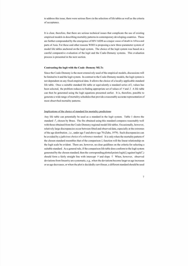
Implications of the choice of standard for mortality predictions

Any life table can potentially be used as a standard in the logit system. Table 1 shows the

standard l s x chosen by Brass. The fits obtained using this standard compares reasonably well

with those obtained from the Coale-Demeny regional model life tables. Occasionally, however,

relatively large discrepancies occur between fitted and observed data, especially at the extremes

of the age distribution , i.e., under age 5 and above age 70 (Zaba, 1979). Such discrepancies can

be avoided by a judicious choice of a reference standard. It is only when the mortality pattern of

the chosen standard resembles that of the comparison l x function will the linear relationship on

the logit scale be evident. There are, however, no clear guidlines on the criteria for selecting a

suitable standard. As a general rule, if the comparison life table does conform to the logit system

generated by the chosen standard, then the corresponding plotted points logit(l x) against logit(l s x)

should form a fairly straight line with intercept " and slope $ . When, however, observed

deviations from linearity are systematic, e.g., when the deviations become larger as age increases

or as age decreases, or when the plot is decidedly curvilinear, a different standard should be used



8

(UN, 1983). In appropriate cases, regression technmiques may be used to obtain the parameters

of the best fitting line.

Choosing standards for the WHO system of MLT

In selecting a standard for the WHO system of model life tables, the choices were between (i)

country-specific standard life table, (ii) a global standard life table, and (iii) a standard life table

based on WHO mortality strata (see Appendix A). For the country-specific standard, the life

table for the latest available year for each country was chosen. The global standard was based on

UN data from the 1998 revision of the World Population Prospect. The standards based on the

WHO mortality strata are from historical series and rely on several age patterns of mortality for

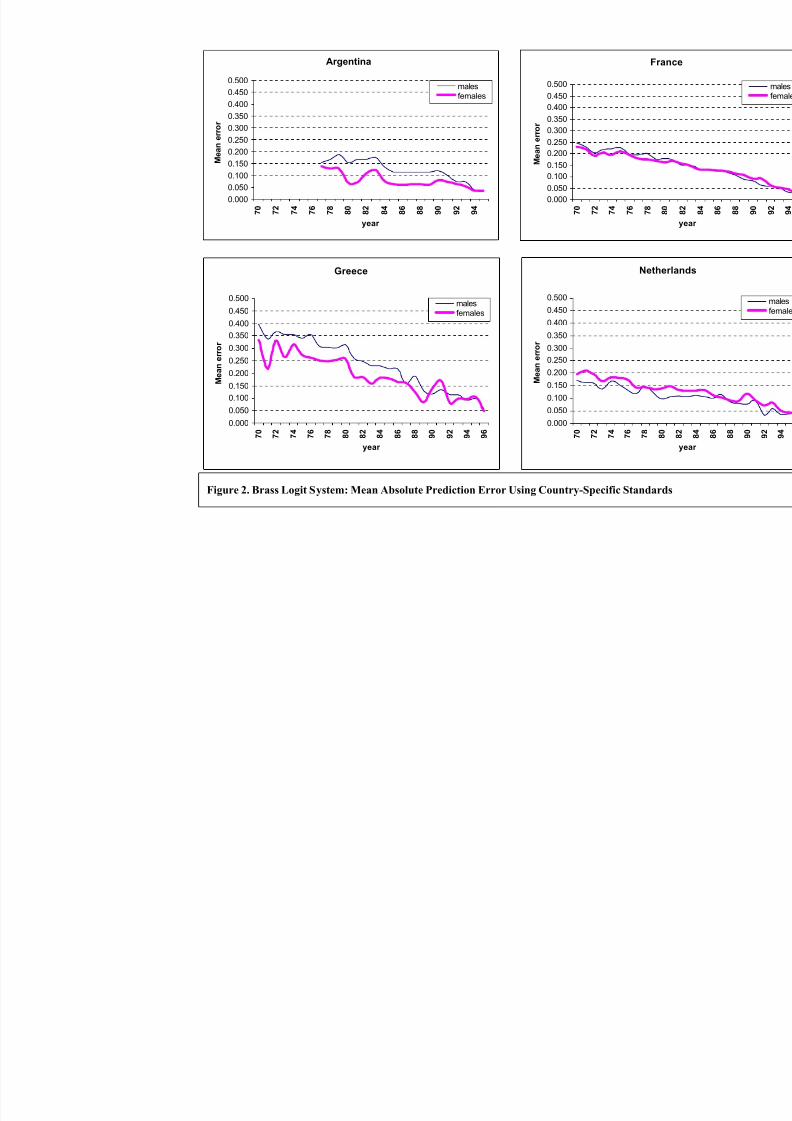
different kinds of populations. In order to objectively compare each of these standards, the mean

absolute deviation (or error) between the observed (real data) and predicted nq x, for a given

standard, were computed over the entire age range, for time series of data for France, Argentina,

Greece and the Netherlands.

In assessing the mean error using the country-specific standard, the following index was used:

where n is the number of age groups in each life table. A plot of the mean error over time for

France, Argentina, Greece and the Netherlands are shown in Figure 2. The results show that,

within the time series for any given country, the mean error for a prediction becomes smaller the

closer the time location of the standard relative to the predicted life table. The plots also show

marked variation in the size of the mean prediction error between countries. Hence, for the

purposes of international comparison, the use of country-specific standards is likley to produce

incomparable results depending on the age pattern of mortality in each country relative to the

standard. A "neutral" standard that is not based on the experience of any particular country will,

therefore, be preferable.

The choice is then between a single global standard and a set of region-specific standards based

on the WHO mortality strata. There are of course comparability issues surrounding the use of

regional standards, but these are no different from those concerning the use of different families

of the Coale-Demeny model life tables. The results of this comparison are shown in Figure 3 for Argentina (1977, 1985 and 1996) using Amr B standard, France (1970, 1985, 1996) and Greece

Mean absolute deviation

q

q

n

n x

n x

=

-æ

è ç

ö

ø÷å 1

$



9

(1970, 1985 and 1977) using Eur A standard, and for Poland(1970, 1985 and 1996) Using Eur B

standard. In general, the global standard tends to produce over-estimates of the age-specific

mortality rates at the extremes of the age range. This is particularly true in France, Greece and

Argentina, probably reflecting the younger age distribution of the standard relative to the

distributions in these populations. In contrast, the WHO regional mortality standards tend to

yield smaller mean errors. In the case of Argentina and Greece, the regional standards tend to

produce higher age-specific mortality rate between age 15 and 40 years. In the case of Poland,

the age pattern produced by the WHO regional standard closely approximates that of the global

standard. Thus relative to the global standard, the WHO regional standards tend to produce

smaller age-specific bias.

In summary, country-specific standards are ideal for country-specific comparisons. However, for international comparison, a neutral standard has obvious advantages. While a global standard

would have been preferable, it appears to be strongly influenced by the relative age pattern of

mortality at the extremes of the age range. In contrast, the regional standards tend to yield

smaller biases although, issues of comparability across regions must be taken into consideration

in interpreting results. After considering these issues, the WHO regional mortality standards

were chosen for subsequent analysis.

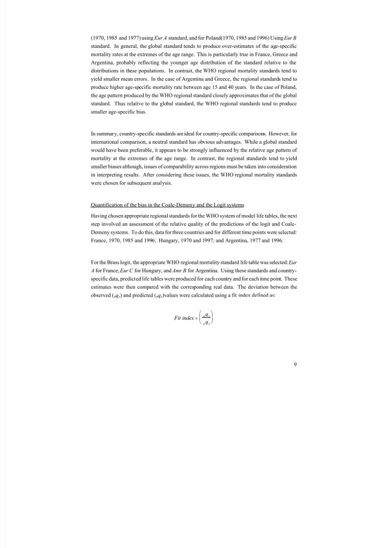
Quantification of the bias in the Coale-Demeny and the Logit systems

Having chosen appropriate regional standards for the WHO system of model life tables, the next

step involved an assessment of the relative quality of the predictions of the logit and Coale-

Demeny systems. To do this, data for three countries and for different time points were selected:

France, 1970, 1985 and 1996; Hungary, 1970 and 1997; and Argentina, 1977 and 1996.

For the Brass logit, the appropriate WHO regional mortality standard life table was selected: Eur

A for France, Eur C for Hungary, and Amr B for Argentina. Using these standards and country-specific data, predicted life tables were produced for each country and for each time point. These

estimates were then compared with the corresponding real data. The deviation between the

observed (nq x) and predicted (nq x)values were calculated using a fit index defined as:

Fit indexq

q

n x

n x

=æ

è ç

ö

ø÷

$



10

In each country and for each time point, a Coale-Demeny model life table corresponding to the

observed life expectancy was selected from each of the four families. Each identified life table

was compared with the life table based on real data. The fit index defined above was then used

to assess the deviation between observed and predicted. Figures 4-6 show comparison plots of

the age-specific devations due to the logit system and those due to the Coale-Demeny models for

each country and for each time point. The West and East families of the Coale-Demeny model

produce better overall fit to the data than the North and South, especially at the younger ages, 0-

15 years. The logit system systematically performs better than the Coale-demeny except in the

case of Argentina, where both systems do relatively poorly. In particular, the logit system tends

to over-estimate mortality while the Coale-Demeny under-estimates mortality. In France, the fit

produced by the logit system are practically similar to those from the East and West models,

except at the very youngest ages. In Argentina, the Coale-Demeny East and West models

significantly over-estimate mortality below age fifteen years.

In summary, the Coale-Demeny model life tables tend to exaggerate mortality at the younger

ages, especially in the case of the North and South models. In contrast, the Brass logit system

tends to produce better fit except in the case of Argentina, where both the Coale-Demeny and the

logit systems perform poorly. The logit system tends to fit poorly at the extremes of the age

range. This is probably a consequence of the age pattern of mortality implied by the standard.

However, the results vary significantly, with the time location of the observed data relative to the

standard. The more recent the data, the worse the predictions of both the logit and the Coale-

Demeny models, further emphasizing the caution needed in using these models in predicting

contemporary mortality schedules.

WHO system of model life tables

A desirable property of any new model life table will be a capacity to adequately reflect the age

patterns of mortality found in contemporary populations without being constrained to represent

exclusively the patterns in the data used to construct it. This is a specific advantage of the Brass

logit system, which makes it possible to construct logit model life tables with enough parameters

to provide greater accuracy in describing observed patterns of mortality (Brass, 1977; Zaba,

1979; Ewbank et al ., 1983). An important question though, is whether it is possible to construct

models with fewer parameters than the four or five parameter dimensions needed for greater

accuracy? Is it possible to identify parsimonius models whose relatively few parameters can be

selected on the bases of knowledge of auxilliary variables?



11

In attempting to answer these questions, we explored the relationship between under-five

mortality (5q0) and adult mortality (45q15) using the attractive properties of the logit scale. These

variables are known life table functions that are easily estimated, and many recent surveys

include questions designed to collect the necessary data for their calculation. An underlying

principle for the WHO system of model life tables is that, knowledge of the values of these two

auxilliary variables (5q0 and 45q15) and an appropriate regional standard life table should uniquely

define the set of " and $ parameters for a unique life table. One can then generate life tables for

any contemporary population.

Construction of the WHO system of MLTs

The WHO system of model life tables is a graphical extension of the Brass logit system anchored

on the relationship between under-five mortality and adult mortality, within a space whose

coordinates are defined by the coefficients of the logit equation, i.e., the " and $ parameters

corresponding to a given standard. The x-axis and y-axis reprsent the " and the $ values,

respectively. For each standard mortality schedule, e.g., the Eur A standard, isobars of 5q0 and

45q15 are plotted within the logit space according to the following equations:

where k=45q15 , c15=logit(l 15 Eur A

), c60=logit(l 60 Eur A

),l 5 and l 5 EurA

are constants. Also l 5 and l 5 EurA

are the probabilities of surviving to age 5 years in the life table of interest and the Europe A

standard life table, respectively. By definition, the isobars for the under-five mortality are linear

while those for the adult mortality are curvilinear. The detailed algebraic derivations of the above

equations are presented in the appendices B and C. In constructing the isobars for any given

value of under-five mortality, hypothetical values of b (e.g., from 0.2 to 1.4) are substituted in

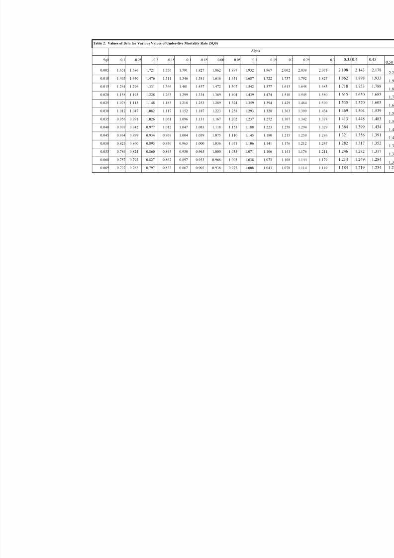
the first equation to obtain corresponding values of a on the given standard (Table 2). Similarly,

to construct an isobar for a given value of adult mortality (k ), different hypothetical values of $

are substituted in the second equation to obtain correspoding vales of " (Table 3).

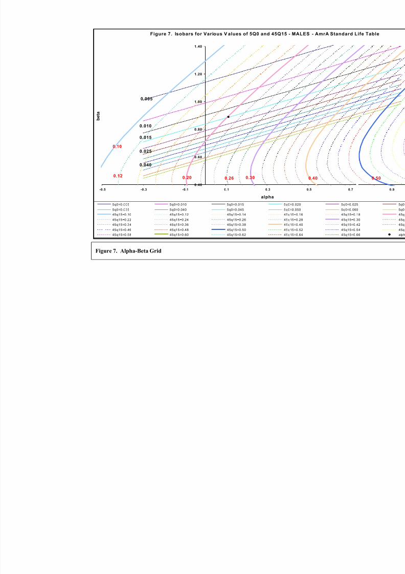
The paired (",$) values at any given level of under-five or adult mortality are plotted on the",$

grid. Points corresponding to the same level of mortality are then joined to form the isobars

(Figure 7). Figure 7 shows a detailed plot of the output grid from this model for the WHO Amr A

( ) ( )

( )

For q the general equation for the isobar is

it l it l

For q the general equation for the isobar isk

k e e

EurA

c c

5 0

5 5

45 15

0 51 60 15

a b

a b b

= -

=- -

é

ëê

ù

ûú

log log

. ln



12

standard life table. Isobars of constant child mortality (lines slanting from bottom left to upper-

right corner on the figure) and constant adult mortality (curves with convexity to the left) are

shown in fine gradations for values of 5q0 ranging from 0.005 to 0.065, and for values of 45q15

ranging from 0.1 to 0.66. Depending on need, the finer gradations may or may not be plotted

(see Figure 9).

The ",$ Grid

The point of intersection between an isobar for child mortaity and one for adult mortality

uniquely defines a life table. Thus, to estimate a life table for the population under study, the

point on the grid defined by values of 5q0 and 45q15 for a population is located, and the

corresponding values of " and $ are then read off corresponding axes. The ",$ pair

corresponding to this point and the age-specific logit values corresponding to the appropriate

WHO regional standard mortality schedule are substituted in the logit equation for that region to

generate a complete life table. As an example, suppose that values of 5qo and 45q15 are available

for a country from a demographic survey or from intercensal survival analysis. If these were

estimated at 20/1000 and 170/1000 respectively, then locating this point (marked with an *) on

Figure 7, and reading across and down to the axes, suggests a value of " = 0.11 and $ = 0.89.

Applying these values in the logit equation with the specified regional standard yields the

schedule of l x values at all ages.

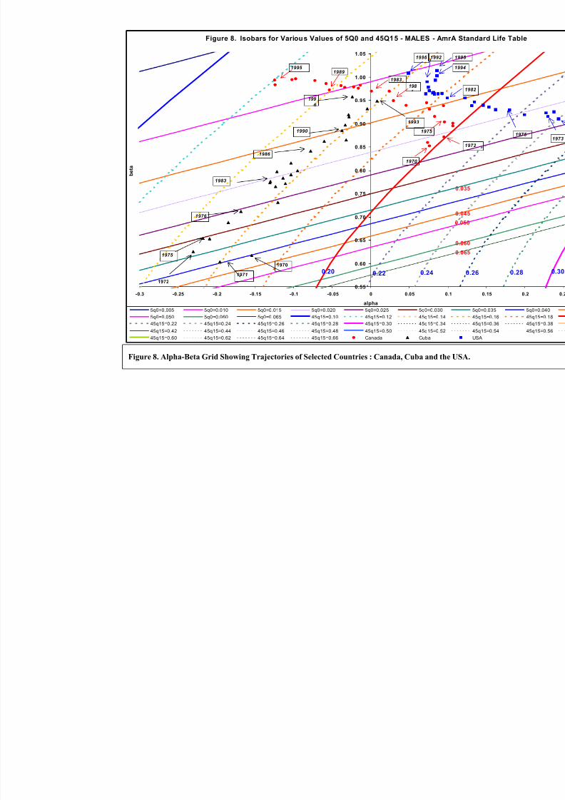
The plot also shows that as adult mortality levels decline, adult mortality isobars shift to the left

along a line at a positive angle to the x-axis ("-axis). In other words, both " and $ decrease in

value with decline in adult mortality. In contrast, " decreases but $ increases in value as child

mortality declines, albeit slowly. The child mortality isobars move to the left along a line at a

negative angle to the x-axis ("-axis).

For any given population and standard, a time series of points defined by " ,$ pairs represent themortality trajectory of that population over time. Figure 8 shows the trajectories for Canada,

Cuba and USA using Amr A standard life table. The USA and Canada show a sustained decline

in both adult and child mortality, with later slowdown in child mortality (at very low levels) in

the most recent period. Cuba demonstrates a substantial decline in child mortality with minimal

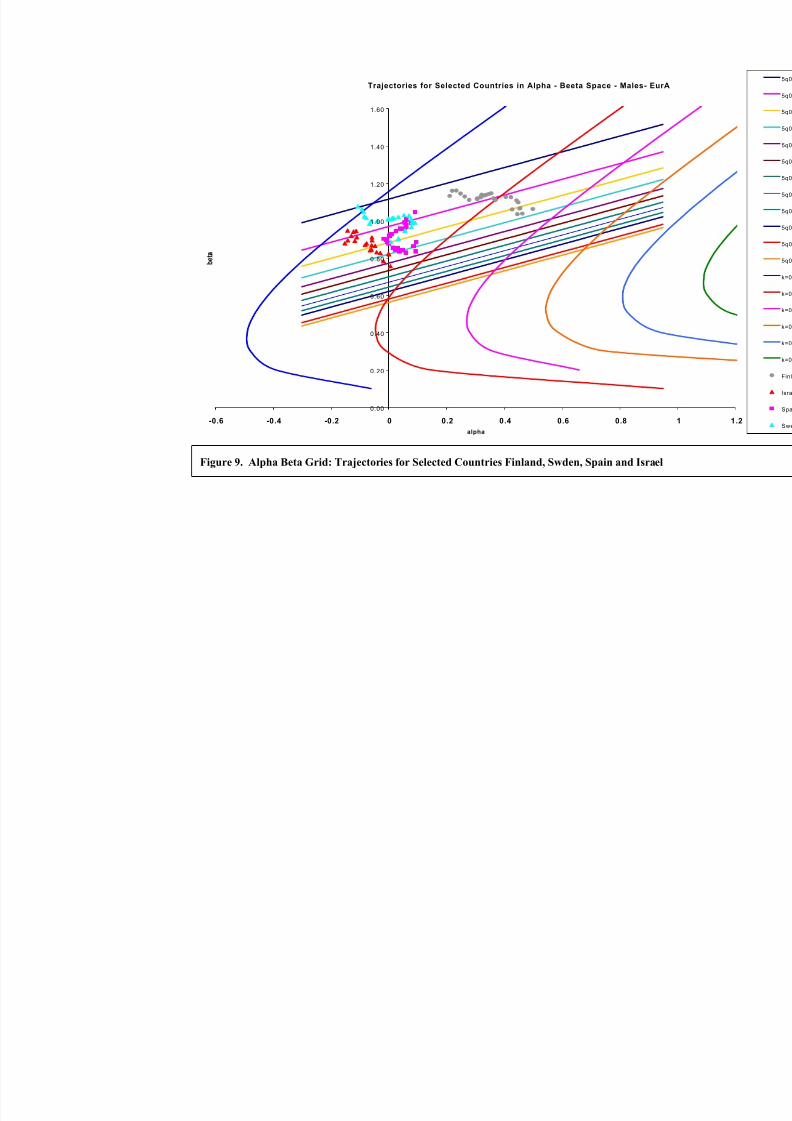
change in adult mortality. Figure 9 shows similar plots for Finland, Sweden, Spain and Israel.

Spain shows a historical pattern of decline in both adult and child mortality followed by contined

decline in child mortality but relatively little change in adult mortality. The plot for Sweden

shows two phases: an earlier phase of substantial decline in adult mortality with relatively littlechange in child mortality, followed by a second phase characterized by decline in both adult and



13

child mortrality. Finland shows a substantial decline in adult mortality with only marginal

change in child mortality at very low levels.

To summarize, in circumstances where an historical sequence of life tables are available it is

possible to generate a time series of a , b pairs using either a country-specific standard or a WHO

regional mortality standard. A plot of a and b , separately, against time should produce a

trajectory of points (see Lopez et al ., 2000). If the plot of points for each parameter fall along a

fairly straight line, that line could theoretically be projected forward to forecast estimates for any

time in the future. These a,b estimates can then be substituted into the appropriate logit

equations to obtain the corresponding life tables. Alternatively, it is possible to plot the a,b

pairs of points on the a,b grid corresponding to a particular WHO reference standard (see

Figures 8 and 9). The trajectory of such points could then be projected forward to obtainestimates of a and b. The disadvantage of this approach is that, it is not easy to assign a time

location to the life table generated.

In the absence of an historical trajectory, a life table may also be defined by first estimating 5q0

and 45q15 in the year of interest and then locating the point of intersection between the isobars

corresponding to these values of 5q0 and 45q15. The finer the gradations of the isobars the better

the predictions. Wide gradations lead to greater uncertainty. Using this method, the level of

uncertainty in the estimates of 5q0 and 45q15 may be translated into uncertainty around the life

table. For example, probability distributions around 5q0 and 45q15 may be defined, and multiple

life tables generated using Monte Carlo simulation methods. The range of life tables may then

represent the probability distribution of predicted age-specific mortality patterns given uncertain

summary measures of child and adult mortality. For more details refer to Salomon and Murray

(2000).

Discussion

The logit system for developing life tables has a number of intuitively appealing characteristics.

To begin with, the system is not dependent on the existence of a large empirical database of age-

specific mortality rates which are required to effectively model age-patterns of mortality. This is

particularly relevant for regions where reliable estimates of age-specific death rates may be

available for only a few countries, and then for only a few periods. The model does not assume

any a priori knowledge about the form of the relationship between age-specific death rates.

Rather, the statistical property of linearity in logits is atheoretical and invariant across mortality

patterns.



14

The higher degree of parametization in the WHO system (3 parameters: " ,$ and the choice of

standard) compared with the empirical systems of model life tables can also be expected to

provide a more robust basis for estimating mortality patterns and levels. The parameters" and$

are also readily interpretable. " varies around a central value of 0, with values greater than zero

indicating progressively higher mortality overall relative to the standard, and values below zero

the opposite. For $ , a reasonable range of values appear to be from about 0.6 to 1.4 (Newell,

1988 ), depending on the standard. Low values of $ suggest high infant and child mortality

relative to the standard, whereas high values imply the reverse (i.e. lower child, higher adult

mortality relative to the standard). (Note that choosing a value of $ = 1.0 reduces to a one-

parameter (" ) system, similar to the level parameter of conventional Coale-Demeny model life

table systems).

As overall population health improves, one would expect values of " to decrease. The trends in

$ are more difficult to predict and depends very much on the standard. Thus in the case of a

standard with relatively high mortality at younger ages, the age at which half the births exposed

to the standard mortality rates will survive is relatively low. Below this age, declining mortality

would result in b increasing, but decreasing above this age. As the standard migrates towards a

lower mortality set of l x’s, the median age of survival rises, often to age 80 or higher. As a result,

b tends to increase as mortality declines, as has been observed in the more developed countries

with low mortality standards over the past few decades.

Although data on child mortality are becoming increasingly available, reliable estimates of adult

mortality are much less common. Considerable uncertainty remains as to current adult mortality

levels, particularly in populations with high prevalence of HIV/AIDS. Using the methods

described in this paper, we have developed a new set of life tables that take into account the best

available data on child and adult mortality, while at the same time reflecting the different levels

of uncertainty around each of these inputs, and across different countries. Ranges of uncertainty

around the life tables were derived using simulation techniques, which allow the level of uncertainty around 5q0 and 45q15 to be translated easily into uncertainty around the ultimate

quantities of interest. In the World Health Report 2000, we report both the point estimates and

the uncertainty intervals for a variety of measures computed from the life tables, including life

expectancy at birth and disability-adjusted life expectancy, as described elsewhere. We believe

strongly that communicating this uncertainty is as critical as communicating point estimates.

Examining the level of uncertainty in each country helps to highlight the major challenges for

demographic estimation and to identify priorites for accelerating survey programmes and sentinel

surveillance in developing countries.



15

References

Gompertz B (1825). On the Nature of the Function Expressive of the Law of Human

Mortality; and on a New Mode of Determining the Value of Life Contingencies,

Philosophical Transactions of the Royal Society, Vol. 115, No. 27, Pp. 513-585.

Keyfitz N (1984). Choice of Function for Mortality Analysis: Effective Forecasting

Depends on a Minimum Partameter Representation, in Vallin, J., J,H, Pollard, and L.

Heligman (Eds.), Methodologies for the Collection and Analysis of Mortality Data.

IUSSP, Ordina Editions. Liege, Belgium. Pp. 225-241.

Coale AJ & Demeny P (1966). Regional Model Life Tables and Stable Population,

Princeton University Press, Princeton, N.J. 1966.

United Nations (1955). Age and Sex Patterns of Mortality: Model Life Tables for Under-Developed Countries. Population Studies, No. 22. Department of Social Affairs.

Sales No. 1955.XIII.9.

United Nations (1967). Methods for Estimating Basic Demographic Measures from

Incomplete Data: Manuals and Methods of Estimating Populations. Manual IV.

Population Studies, No. 42. Department of Economic Social Affairs. Sales No. 1967.

XIII.2

United Nations (1956). Manual III: Methods for Population Projections by Sex and

Age. United Nations Publications, Sales No. 1956.XIII.3.

Demeny P & Shorter FC (1968). Estimating Turkish Mortality, Fertility and Age

Structure. Istanbul, Istanbul University, Statistics Institute.

Ledermann S & Breas J (1959). Les Dimensions de la Mortalité. Population, Vol. 14,

No. 4., Pp. 637-682. Paris.

Ledermann S (1969). Nouvelles Tables-type de Mortalité. Traveaux et Document ,

Cahier No. 53. Paris, Institut National d’études Démographiques.

Brass W. et al (1968). The Demography of Tropical Africa. Princeton, Princeton

University.

Brass W (1971). On the Scale of Mortality, in W. Brass (ed.), Biological Aspects of

Demography. London: Taylor & Francis.

Carrier NH & Hobcraft J (1971). Appendix 1, Brass Model Life Table System, in

Demographic Estimation for Developing Societies, London: Population Investigation

Committees.

United Nations (1981). Model Life Tables for Developing Countries. United NationsPublication, Sales No. E.1981.XIII.7.



16

Menken J (1977). Current Status of Demographic Models, in Meetings of the ad hoc

Group of Experts on Demographic Models. Population Bulletin of the United Nations.

Vol. 9. Pp.22-34.

United Nations (1977). Demographic Models, in Meetings of the ad hoc Group of Experts on Demographic Models. Population Bulletin of the United Nations. Vol. 9.

Pp.11-26.

Zaba B (1979). The Four-Parameter Logit Life Table System. Population Studies, Vol.

33, No. 1. March. 1979. Pp. 79-100.

United Nations (1983). Manual X: Indirect Techniques for Demographic Estimation.

Department of International Economic and Social Affairs. Population Studies, No. 81.

ST/ESA/SER.A/81. United Nations Publication. Sales No. E.83.XIII.2.

Ahmad OB, Lopez AD & Inoue M (2000). Trends in Child Mortality: A Reappraisal.

Bulletin of the World Health Organizat, Vol. ?. No. ? (Forthcoming – September, 2000).

Newell C (1988). Methods and Models in Demography. The Guilford Press.

Eubank DC, Gomez de Leon JC, & Stoto MA (1983). A Reducible Four Parameter

System of Model Life Tables, Population Studies 37, Pp. 105-127.

Brass W (1977). Notes on Empirical Models, in Meetings of the ad hoc Group of

Experts on Demographic Models. Population Bulletin of the United Nations. Vol. 9.

Pp.38-42.



Table 1. Logit Values of the Brass General Standard Life Table

Age

(x) l x Logit

Value

Age

(x) l x Logit

Value

Age

(x) l x Logit

Value

Age

(x) l x Logit

Value

Age

(x)

l x

0 1.000

1 0.850 -0.867 21 0.707 -0.440 41 0.583 -0.167 61 0.383 0.2394 81 0.0

2 0.807 -0.715 22 0.700 -0.425 42 0.576 -0.153 62 0.368 0.2701 82 0.0

3 0.788 -0.655 23 0.694 -0.410 43 0.569 -0.138 63 0.345 0.3204 83 0.0

4 0.776 -0.622 24 0.688 -0.396 44 0.561 -0.123 64 0.338 0.3364 84 0.0

5 0.769 -0.602 25 0.683 -0.383 45 0.553 -0.107 65 0.322 0.3721 85 0.0

6 0.764 -0.588 26 0.676 -0.369 46 0.545 -0.091 66 0.306 0.4097 86 0.0

7 0.760 -0.577 27 0.670 -0.355 47 0.537 -0.075 67 0.289 0.4494 87 0.0

8 0.756 -0.567 28 0.664 -0.341 48 0.529 -0.057 68 0.272 0.4912 88 0.0

9 0.753 -0.558 29 0.658 -0.328 49 0.520 -0.040 69 0.255 0.5353 89 0.0

10 0.750 -0.550 30 0.652 -0.315 50 0.511 -0.021 70 0.238 0.5818 90 0.0

11 0.748 -0.543 31 0.647 -0.302 51 0.501 -0.002 71 0.221 0.6311 91 0.0

12 0.745 -0.537 32 0.641 -0.289 52 0.491 0.018 72 0.203 0.6832 92 0.0

13 0.743 -0.530 33 0.635 -0.276 53 0.481 0.038 73 0.186 0.7385 93 0.0

14 0.740 -0.522 34 0.628 -0.263 54 0.470 0.060 74 0.169 0.7971 94 0.0

15 0.736 -0.513 35 0.622 -0.250 55 0.459 0.082 75 0.152 0.8593 95 0.0

16 0.733 -0.504 36 0.616 -0.236 56 0.447 0.106 76 0.136 0.9255 96 0.0

17 0.729 -0.494 37 0.610 -0.223 57 0.435 0.130 77 0.120 0.9960 97 0.0

18 0.724 -0.482 38 0.603 -0.209 58 0.423 0.155 78 0.105 1.0712 98 0.0

19

0.719 -0.469 39 0.597 -0.196 59 0.410 0.182

79

0.091 1.1516 99 0.0

20 0.713 -0.455 40 0.590 -0.182 60 0.397 0.210 80 0.078 1.2375



Table 2. Values of Beta for Various Values of Under-five Mortality Rate (5Q0)

Alpha

5q0 -0.3 -0.25 -0.2 -0.15 -0.1 -0.05 0.00 0.05 0.1 0.15 0.2 0.25 0.3

0.005 1.651 1.686 1.721 1.756 1.791 1.827 1.862 1.897 1.932 1.967 2.002 2.038 2.073

0.010 1.405 1.440 1.476 1.511 1.546 1.581 1.616 1.651 1.687 1.722 1.757 1.792 1.827

0.015 1.261 1.296 1.331 1.366 1.401 1.437 1.472 1.507 1.542 1.577 1.613 1.648 1.683

0.020 1.158 1.193 1.228 1.263 1.299 1.334 1.369 1.404 1.439 1.474 1.510 1.545 1.580

0.025 1.078 1.113 1.148 1.183 1.218 1.253 1.289 1.324 1.359 1.394 1.429 1.464 1.500

0.030 1.012 1.047 1.082 1.117 1.152 1.187 1.223 1.258 1.293 1.328 1.363 1.399 1.434

0.035 0.956 0.991 1.026 1.061 1.096 1.131 1.167 1.202 1.237 1.272 1.307 1.342 1.378

0.040 0.907 0.942 0.977 1.012 1.047 1.083 1.118 1.153 1.188 1.223 1.258 1.294 1.329

0.045 0.864 0.899 0.934 0.969 1.004 1.039 1.075 1.110 1.145 1.180 1.215 1.250 1.286

0.050 0.825 0.860 0.895 0.930 0.965 1.000 1.036 1.071 1.106 1.141 1.176 1.212 1.247

0.055 0.789 0.824 0.860 0.895 0.930 0.965 1.000 1.035 1.071 1.106 1.141 1.176 1.211

0.060 0.757 0.792 0.827 0.862 0.897 0.933 0.968 1.003 1.038 1.073 1.108 1.144 1.179

0.065 0.727 0.762 0.797 0.832 0.867 0.903 0.938 0.973 1.008 1.043 1.078 1.114 1.149



Figure 1. Effect of Changing Alpha and Beta on Pattern of Observed Mortality Relative to Standa

Effect of Varying Be ta at a Fixed Alpha Parame ter

-6.0

-5.0

-4.0

-3.0

-2.0

-1.0

0. 0

1.0

2. 0

3. 0

-3.0 -2.0 -1.0 0 .0 1.0 2.0 3.0

Logit (standard)

L o g i t ( o b s e r v e d )

b=0.2 b=0.4 b=0.6 b=0.8

b=1.0 b=1.2 b=1.4

Effect of Varyin g Alpha at

-2.5

-2.0

-1.5

-1.0

-0.5

0.0

0.5

1.0

1.5

2.0

2.5

-3 .0 -2.0 -1.0

Logit (st

L o g i t ( o b s e r v e d l x )

a=-1.5 a=-1.0a=0.5 a=1.0

Variation in Beta at Con stant Alpha

0.00

0.10

0.20

0.30

0.40

0.50

0.60

0.70

0.80

0.90

1.00

- 10 20 30 40 50 60 70 80 90

Age

S u r v i v o

r s h i p

beta=0.8 b=0.6 b=0.4 Standard

Variation in Alpha

0.0000

0.2000

0.4000

0.6000

0.8000

1.0000

1.2000

- 10 20 30 40

A

S u r v i v a l

Standard a=0.2

a=.8 a=1.0



Franc

0.000

0.050

0.100

0.150

0.200

0.250

0.300

0.350

0.400

0.450

0.500

7 0

7 2

7 4

7 6

7 8

8 0

M e a n e r r o r

Argentina

0.000

0.050

0.100

0.150

0.200

0.250

0.300

0.350

0.400

0.450

0.500

7 0

7 2

7 4

7 6

7 8

8 0

8 2

8 4

8 6

8 8

9 0

9 2

9 4

year

M e a n e

r r o r

malesfemales

Greece

0.000

0.050

0.100

0.150

0.200

0.250

0.300

0.350

0.400

0.450

0.500

7 0

7 2

7 4

7 6

7 8

8 0

8 2

8 4

8 6

8 8

9 0

9 2

9 4

9 6

year

M e a n e r r o r

malesfemales

Netherla

0.000

0.050

0.100

0.150

0.200

0.250

0.300

0.350

0.400

0.450

0.500

7 0

7 2

7 4

7 6

7 8

8 0

M e a n e r r o r

Figure 2. Brass Logit System: Mean Absolute Prediction Error Using Country-Specific Standards



Fr

-0.5

0

0.5

1

1.5

2

2.5

3

3.5

4

a

Argentina

-0.5

0

0.5

1

1.5

2

2.5

3

3.5

4

0 1 5 10 15 20 25 30 35 40 45 50 55 60 65 70 75 80 85+age- gro up

1977 using Amr B98 as stand

1977 using Global98 as stand





Greece

-0.5

0

0.5

1

1.5

2

2.5

3

3.5

4

0 1 5 10 15 20 25 30 35 40 45 50 55 60 65 70 75 80 85+age-group

1970 using EurA98 a s stand

1970 using Global98 sta nd.

1985 using EurA98 a s stand.


1997 using EurA98 a s stand.

1997 using Global98 as stand.

P

-0.5

0

0.5

1

1.5

2

2.5

3

3.5

4

0 1 5 10 15 20 25 30

Figure 3. Brass Logit System: Mean Prediction Error in nqx - WHO Regional Standard Versus a Gl



North model

0. 000

1. 000

2. 000

3. 000

4. 000

5. 000

6. 000

7. 000

8. 000

9. 000

0 1 5 10 15 20 25 30 35 40 45 50 55 60 65 70 75 80 85+

age-gr oup

1970 Logit

1997 Logit

1970 C-D (North)

1997 C-D (North)

South mode

0. 000

1. 000

2. 000

3. 000

4. 000

5. 000

6. 000

7. 000

8. 000

9. 000

0 1 5 10 15 20 25 30 35

age

East model

0 . 000

1.000

2 . 000

3 . 000

4 . 000

5 . 000

6 . 000

7 . 000

8 . 000

9 . 000

a g e - g r o u p

1970 Logit

1997 Logit

1970 C-D (East)

1997 C-D (East)

West mo

0 . 000

1.000

2 . 000

3 . 000

4 . 000

5 . 000

6 . 000

7 . 000

8 . 000

9 . 000

a g e

Figure 4. Index of Fit - Brass Logit and the Coale-Demeny Models - Hungary - Males, by Age and



South mod

0. 00

0. 50

1. 00

1. 50

2. 00

2. 50

3. 00

3. 50

4. 00

4. 50

5. 00

5. 50

6. 00

6. 50

7. 00

0 1 5 1 0 1 5 2 0 2 5 3 0 3 5 age-

West mode

0. 00

0. 50

1. 00

1. 50

2. 00

2. 50

3. 00

3. 50

4. 00

4. 50

5. 00

5. 50

6. 00

6. 50

7. 00

0 1 5 1 0 1 5 2 0 2 5 3 0 3 5

age

North mode l

0 . 0 0

0 . 5 0

1 . 00

1 . 50

2 . 0 0

2 . 5 0

3 . 0 0

3 . 5 0

4 . 0 0

4 . 5 0

5 . 0 0

5 . 5 0

6 . 0 0

6 . 5 0

7 . 0 0

age - gr oup

1970 Logit1985 Logit1996 Logit1970 C-D (North)1985 C-D (North)1996 C-D (North)

East m odel

0 . 0 0

0 . 5 0

1 . 00

1 . 50

2 . 0 0

2 . 5 0

3 . 0 0

3 . 5 0

4 . 0 0

4 . 5 0

5 . 0 0

5 . 5 0

6 . 0 0

6 . 5 0

7 . 0 0

age - gr oup

1970 Logit1985 Logit1996 Logit1970 C-D (East)1985 C-D (East)1996 C-D (East)

Figure 5. Index od Fit - Brass Logit and the Coale-Demeny Models - France - Males, by Age and T



Figure 8. Alpha-Beta Grid Showing Trajectories of Selected Countries : Canada, Cuba and the USA.

Figure 8. Isobars for Various Values of 5Q0 and 45Q15 - MALES - AmrA Standa

0.55

0.60

0.65

0.70

0.75

0.80

0.85

0.90

0.95

1.00

1.05

-0.3 -0.25 -0.2 -0.15 -0.1 -0.05 0 0.05 0.1

alpha

b e t a

5q0=0.005 5q0=0.010 5q0=0.015 5q0=0.020 5q0=0.025 5q0=0.030 5q0=

5q0=0.050 5q0=0.060 5q0=0.065 45q15=0.10 45q15=0.12 45q15=0.14 45q1

45q15=0.22 45q15=0.24 45q15=0.26 45q15=0.28 45q15=0.30 45q15=0.34 45q1

45q15=0.42 45q15=0.44 45q15=0.46 45q15=0.48 45q15=0.50 45q15=0.52 45q1

45q15=0.60 45q15=0.62 45q15=0.64 45q15=0.66 Canada Cuba USA

1970

1971

1972

1975

1976

1983

1986

1990

1996

1993

1982

1994

1996 1995 1992

1970

1972

1975

198

1983

19891995

0.065

0.060

0.050

0.045

0.035

0.20 0.260.240.22



Trajectories for Selected Countries in Alpha - Beeta Space - Males- EurA

0.00

0.20

0.40

0.60

0.80

1.00

1.20

1.40

1.60

-0.6 -0.4 -0.2 0 0.2 0.4 0.6 0.8

alpha

Figure 9. Alpha Beta Grid: Trajectories for Selected Countries Finland, Swden, Spain and Israel



29

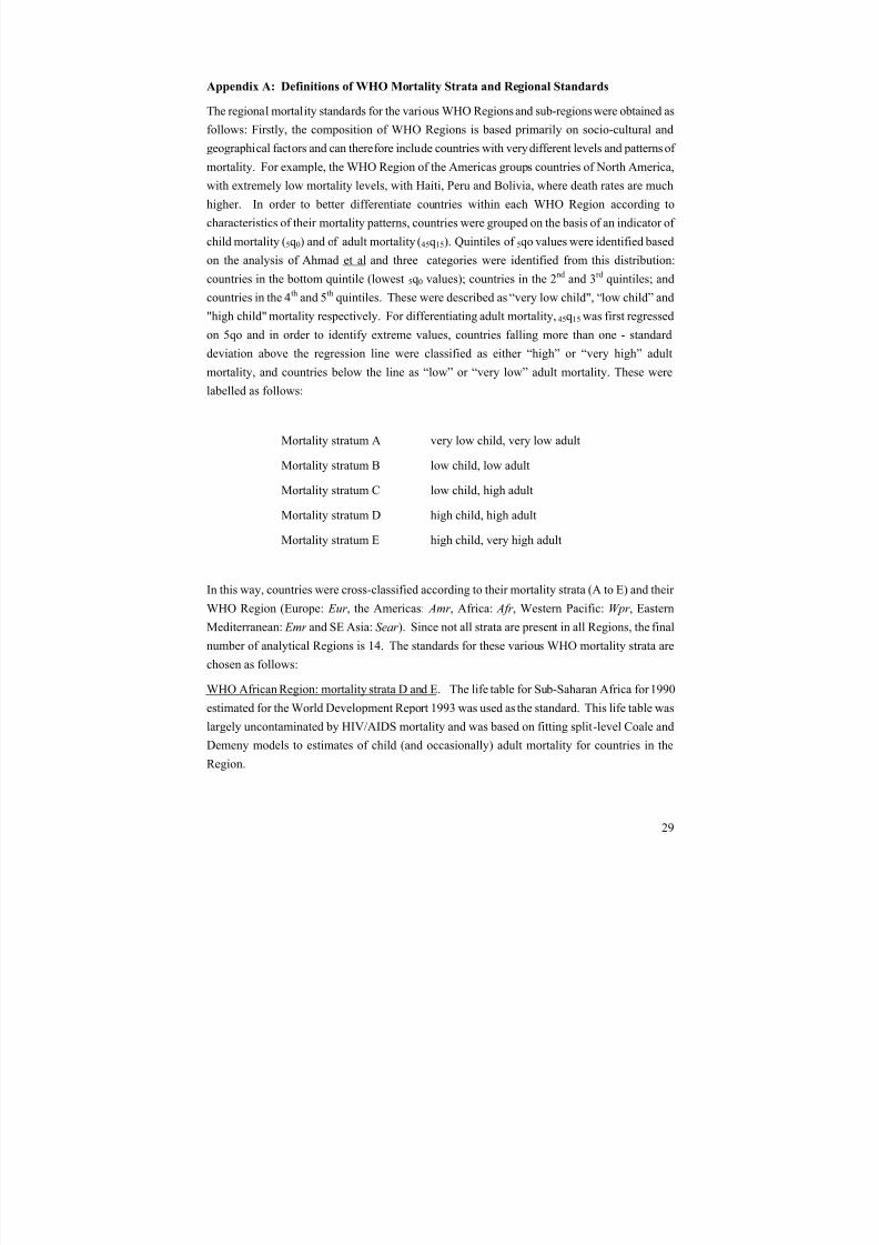
Appendix A: Definitions of WHO Mortality Strata and Regional Standards

The regional mortality standards for the various WHO Regions and sub-regions were obtained as

follows: Firstly, the composition of WHO Regions is based primarily on socio-cultural and

geographical factors and can therefore include countries with very different levels and patterns of mortality. For example, the WHO Region of the Americas groups countries of North America,

with extremely low mortality levels, with Haiti, Peru and Bolivia, where death rates are much

higher. In order to better differentiate countries within each WHO Region according to

characteristics of their mortality patterns, countries were grouped on the basis of an indicator of

child mortality (5q0) and of adult mortality (45q15). Quintiles of 5qo values were identified based

on the analysis of Ahmad et al and three categories were identified from this distribution:

countries in the bottom quintile (lowest 5q0 values); countries in the 2nd

and 3rd

quintiles; and

countries in the 4th and 5th quintiles. These were described as “very low child", “low child” and

"high child" mortality respectively. For differentiating adult mortality, 45q15 was first regressed

on 5qo and in order to identify extreme values, countries falling more than one - standard

deviation above the regression line were classified as either “high” or “very high” adult

mortality, and countries below the line as “low” or “very low” adult mortality. These were

labelled as follows:

Mortality stratum A very low child, very low adult

Mortality stratum B low child, low adult

Mortality stratum C low child, high adult

Mortality stratum D high child, high adult

Mortality stratum E high child, very high adult

In this way, countries were cross-classified according to their mortality strata (A to E) and their

WHO Region (Europe: Eur , the Americas: Amr , Africa: Afr , Western Pacific: Wpr , Eastern

Mediterranean: Emr and SE Asia: Sear ). Since not all strata are present in all Regions, the final

number of analytical Regions is 14. The standards for these various WHO mortality strata are

chosen as follows:

WHO African Region: mortality strata D and E. The life table for Sub-Saharan Africa for 1990

estimated for the World Development Report 1993 was used as the standard. This life table was

largely uncontaminated by HIV/AIDS mortality and was based on fitting split-level Coale and

Demeny models to estimates of child (and occasionally) adult mortality for countries in the

Region.



30

WHO Western Pacific Region: mortality stratum E. The 1990 life table for China prepared for

the WDR 1993 was used. Deaths reported in the previous 12 months from the 1990 census were

adjusted for underreporting using standard demographic procedures.

WHO Eastern Mediterranean Region: mortality strata B and D. Mortality data from Egypt for

1991 and 1992 were averaged and adjusted for underreporting, particularly below age 5, based

on a review of all demographic data sources on child mortality levels in Egypt.

WHO European Region: mortality stratum B : This standard was based on the unweighted

aggregated mortality data for the following countries: Albania (1992-93), Armenia (1995-97),

Azerbaijan (1995-97), Bulgaria (1996-98), Georgia (1988-90), Kyrgystan (1996-98), Poland

(1994-96), Romania (1996-98), Slovakia (1993-95), Tajikistan (1990-92), Macedonia (1995-97),

Turkmenistan (1992-94) and Uzbekistan (1991-93)

WHO South East Asia Region: mortality stratum B. Mortality data for Sri Lanka for 1991 and

1995 were averaged, and added to adjusted mortality data for Thailand (1988-90) and Malaysia

(1974-76), using Growth-Balance to adjust for underreporting.

Mortality stratum D: Indian mortality data for 1995-97 from the Sample Registration Scheme

was used for the standard, with adjustments above age 5 for underreporting (estimated at 13-

14%, using the Bennet-Horiuchi technique).

WHO American Region: mortality stratum B. Based on average mortality rates for Argentina

(1990-96), Bahamas (1993-95), Barbados (1993-95), Belize (1995), Brazil (1996) (with

corrections for underreporting), Chile (1992-94), Columbia (1992-94) (corrected for

underreporting), Costa Rica (1992-94), Jamaica (1983 and 1985), Mexico (1993-95), Panama(1985-87) (adjusted for underreporting), Trinidad and Tobago (1992-94), Uruguay (1988-90)

and Venezuela (1992-94) (with adjustments for underreporting).

Mortality stratum D: historical data for Latin American countries at earlier (higher mortality)

periods were used. These included: Antigua (1970-72),

Argentina (1969-70), Bahamas (1971-72), Barbados (1970-72), Chile (1970-72), Costa Rica

(1970-72), El Salvador (1970-72), Dominican Rep. (1970-72), Mexico (1970-72), Panama(1970-72), Trinidad & Tobago (1970-72), Uruguay (1970-72), Venezuela (1970-72).



31

Appendix B - Derivation of the Equation for the Adult Mortality Isobars

( )

Logit l Logit l

Logit l Logit l

k ql l

l

l k l

s

s

15 15

60 60

45 15

15 60

15

15 60

1

2

3

1

= +

= +

= =-æ

è ç

ö

ø÷

\ - =

a b

a b

KKKKKKKKKK KKKKKK KKKKKKKK

KKKKKKKKKKKK KKK KKKKKKKKK

KKKKKKKKKKKKKKKK KKKKKKK KKK

KKKKKKKKKKKKKKK

. ..

. .

.. ..

( )( )

KKKK KKKKKKKKK

KKKKKKKKKKKKKKK

KKKKKKKKKKKKK KKKKKKKKKKKKK

KKKKKKKKKKKKKKKKKKK KKKKK

. .

,

..

. .

.

4

5

6

4 6

1 7

15 15 60 60

15 15

60 60

60

15 60

If C Logit l and C Logit l then

Logit l C

Logit l C

Substiituting equation for l in equation

Logit l k C

Expanding

s s= =

= +

= +

- = +

a b

a b

a b

( )

( )

the Logits

l

l C

l k

l k C

l

l C

0 51

8

0 51 1

19

12 2 10

15

15

15

15

15

60

15

15

15

. ln . ..

. ln . .

ln ..

ln

-æ

è ç

ö

ø÷ = +

- -

-

é

ëê

ù

ûú = +

-æ

è ç

ö

ø÷ = +

a b

a b

a b

KKKKKKKKKKKKKKK KKKKKKKK

KKKKKKKKKKKK KKKK KKKKK

KKKKKKKKKKKKKKKKKKKKKKKK

( )

( )

( )

1 1

12 2 11

12

1

1

112

15

15

60

15

15

15

2 2 2

15 15

2 2

15 2 2

15

15 15

15

15

- -

-

é

ëê

ù

ûú = +

-æ

è ç

ö

ø÷ = =

\ - =

\ =+

+

l k

l k C

Solving for l

l

l e e e

l l e e

l e e

Substituting for l inequation

C C

C

C

a b

a b a b

a b

a b

KKK KKKKKKKKKKKKKKKKKKK

KKKKKKKKKKKKKKKKK KKKKKKKK

.

. ..

( )

( )

( )

( )( )

( )

( ) ( ){ }( )

( )

( )

( ) ( ){ }( )

11

1 1

1

1

1

1

1

1

1 1

1

1

1

1 1

1

15

15

2 2 2 2

2 2

2 2

2 2

2 2

2 2

2 2

60 60

15

15

15

15

15

15

- -

-

é

ëê

ù

ûú = =

-

-

+-

+

é

ë

êêêê

ù

û

úúúú

=

+ - -

+-

+

é

ë

êêêêê

ù

û

úúúúú

=+ - -

-é

ë

êê

ù

û

+l k

l k e e e

k

e e

k

e e

e e k

e e

k

e e

e e k

k

C C

C

C

C

C

C

C

a b a b

a b

a b

a b

a b

a b

a b

( ) ( ){ } ( )( )

( ) ( )( )

( )( ) ( )

( )( )[ ]

( )( )

úú

=

\ + - - = -

\ + = -

\ - - =

\ - - =

\ =

- -

é

ë

êù

û

ú

e e

e e k k e e

e e k k e e

k e e e e k

e k e e k

k

k e e

C

C C

C C

C C

C C

C C

2 2

2 2 2 2

2 2 2 2

2 2 2 2

2 2 2

2 2

60

15 60

15 60

60 15

60 15

60 15

1 1 1

1

1

1

1

2 1

a b

a b a b

a b a b

a b a b

a b b

b b a ln .KKKKKKKKKKKKK KKKKKKK..13



32

Appendix C: Derivation of the Equation for the Child Mortality Isobars.

( ) ( )

( ) ( )

log log

log log

it l it l

it l it l

s

s

5 5

5 5

= +

\ = -

a b

a b



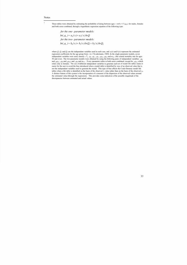
Notes

i These tables were obtained by estimating the probability of dying between ages x and x+5 ( 5q x ), for males, females

and both sexes combined, through a logarithmic regression equation of the following type:

for the one- parameter models:

for the two- parameter models:

ln( ) ( ) ( )ln

ln( ) ( ) ( )ln ( )ln

5 0 1

5 0 1 1 2 2

q a x a x Q

q b x b x Q b x Q

x

x

= +

= + +

where Q, Q1 and Q2 are the independent variables used in each case, and ai(x) and bi(x) represent the estimated

regression coefficients for the age group from x to T (Ledermann, 1969). In the single parameter models, seven

independent variables were used, namely: e00 , 1q0 , 5q0 , 15q0 , 20q30, 20q45 and m50+ (the central mortality rate for ages

50 and over). The two-parameter models were obtained by using the following pairs of independent variables: 5q0

and 20q45; 15q0 and 20q30; and 15q0 and m50+. Every parameter refers to both sexes combined, except for 20q30, which

refers only to females. The use of different independent variables to generate each set of model life tables makes it

easier for the user to avoid the bias introduced when a model table is identified by way of an observed value that is

not the independent variables used to generate the model. This type of bias affects the Coale-Demeny model life

tables when a life table is identified on the basis of the observed l 2 value rather than on the basis of the observed e0.

A distinct feature of this system is the incorporation of a measure of the dispersion of the observed values around

the estimated value (through the regression). This provides some indication of the possible magnitude of the

discrepancies between estimated and actual values.

Who Method for Life Table

Documents

Transcript of Who Method for Life Table