GEOG/GEOL 4093 Remote Sensing of the Environment

Lecture 9

Outline of today’s lecture

• Review

• Imaging Systems- Passive Sensors

• Whiskbroom vs. Pushbroom

• Multi-spectral remote sensing: Landsat (MSS, TM, and ETM+)

Aditive Substractive

Processes in color formation

Additive colors refer to the combination of light from multiple

sources at specific wavelengths

• used in remote sensing, and on computer monitors, etc.

Landsat TM and Color Composites

Band 2 Band 1 Band 3 Band 4 Band 5 Band 6 Band 7

0.450-0.515 µm

(Blue)

0.525-0.605 µm

(Green)

0.63-0.69 µm

(Red)

0.75-0.90 µm

(Near-Infrared)

1.55-1.75 µm

(Middle-Infrared)

2.08-2.35 µm

(Middle-Infrared)

10.40-12.50 µm

(Thermal-Infrared)

Spectral Signature

Spectral Band: A spectral band in a digital image represents a narrow slice of radiance in a given wavelength range. The brightness level in a given spectral band is measured using a sensor that is responsive only in that band or by placing a filter in front of a broad band sensor.

Resolution: Four types of resolutions in remote sensing:

(1) spatial: the smallest angular or linear separation between two objects that can be resolved by the sensor (IFOV).

(2) Temporal: the repeat frequency of information gathered at a specific point.

(3) spectral: the number and dimension of specific wavelength intervals in the EM spectrum to which the instrument is sensitive.

(4) Radiometric: sensitivity of the sensor to different signal strengths.

Imaging Systems

Many electronic (as opposed to photographic) remote sensors acquire data using scanning systems, which employ a sensor with a narrow field of view (i.e. IFOV) that sweeps over the terrain to build up and produce a two-dimensional image of the surface.

There are two main modes or methods of scanning employed to acquire multispectral image data - across-track scanning, and along-track scanning.

Imaging Systems: Whiskbroom Scanners

Across-track scanners scan the Earth in a series of lines. The lines are oriented perpendicular to the direction of motion of the sensor platform (i.e. across the swath). Each line is scanned from one side of the sensor to the other, using a rotating mirror.

Imaging Systems: Whiskbroom Scanners • The IFOV (C) of the sensor and the altitude of the platform determine the ground resolution cell viewed (D), and thus the spatial resolution. The angular field of view (E) is the sweep of the mirror, measured in degrees, used to record a scan line, and determines the width of the imaged swath (F).

• Because the distance from the sensor to the target increases towards the edges of the swath, the ground resolution cells also become larger and introduce geometric distortions to the images.

Whiskbroom Scanners: Dwell Time

• The amount of time a scanner has to collect photons from a ground resolution cell:

(scan time per line)/(#cells per line)

depends on:

– satellite speed

– width of scan line

– time per scan line

– time per pixel

(down track pixel size / orbital velocity)

(cross-track line width / cross-track pixel size)

dwell time =

[(30m / 7500 m/s)/(185000m / 30m)]

=6.5 x 10-7 seconds/pixel

This is a very short time per pixel

Dwell Time Example: Landsat TM

Imaging Systems: Pushbroom Scanners

• Pushbroom scanners use a

linear array of detectors (A) located at the focal plane of the image (B) formed by lens systems (C), which are "pushed" along in the flight track direction (i.e. along track).

• Each individual detector measures the energy for a single ground resolution cell (D) and thus the size and IFOV of the detectors determines the spatial resolution of the system.

Imaging Systems: Pushbroom Scanners

(down track pixel size / orbital velocity)

(cross-track line width / cross-track pixel size)

• denominator = 1.0

• dwell time is longer than that of whiskbroom

• but different response sensitivities in each detector can cause striping in the image

Dwell Time Example: Pushbroom Scanner

Whiskbroom vs. Pushbroom

Wide swath width

Complex mechanical system

Simple optical system

Filters and sensors

Shorter dwell time

Pixel distortion

Narrow swath width

Simple mechanical system

Complex optical system

Dispersion grating and CCDs

Longer dwell time

Less pixel distortion

Whiskbroom vs. Pushbroom

Whiskbroom

• Landsat Multispectral Scanner (MSS)

• Landsat Thematic Mapper (TM)

• Landsat 7 Enhancement Thematic

Mapper (ETM+)

• NOAA Advance Very High Resolution

Radiometer (AVHRR)

• Geostationary Operational

Environmental Satellite (GOES)

Pushbroom

• SPOT S 1,2, and 3 High Resolution

Visible (HRV) . SPOT 4 and 5 (HRVIR)

and Vegetation sensors

• Indian Remote Sensing System (IRS)

• Terra Advance Spacebone Thermal

Emission and Reflection Radiometer

(ASTER)

• Terra Multiangle Imaging

Spectroradiometer (MISR)

• IKONOS , QuickBird

Selected Remote Sensing System and Their characteristics

Adapted from Jensen, 2007

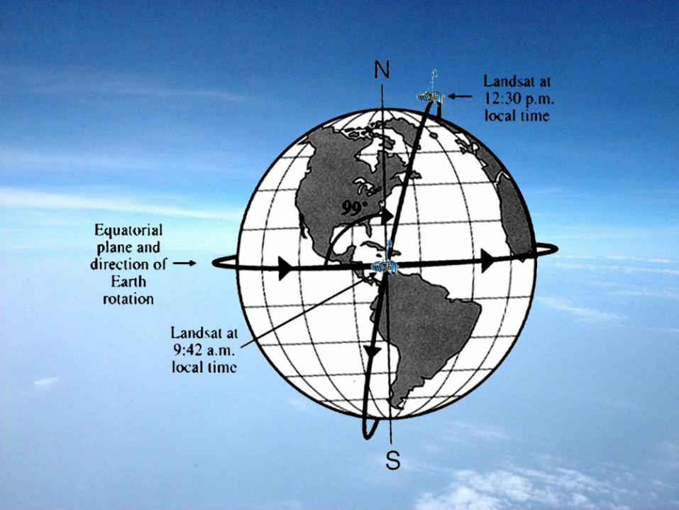
Multi-spectral remote sensing: Landsat (MSS, TM, and ETM+)

• Sun-synchronous near polar orbits

• Inclination 99° and 98.2°

• 919 km altitude (landsat 1, 2, 3), 705 km for the others

• Orbits the earth every 103 minutes (landsat 1, 2, 3)

• Cross latitude at approximately the same local time (equator 9:30 to 10:00 am)

Landsat 1: 1972–1978

Landsat 2: 1975–1982

Landsat 3: 1978–1983

Landsat 4: 1982–2001

Landsat 5: 1984–

Landsat 6: failed launch, 1993

Landsat 7: 1999–

LDCM: Scheduled to launch in December 2012

Multi-spectral remote sensing: Landsat (MSS, TM, and ETM+)

Landsat-1 to 3 Landsat-4 and 5 Landsat-6 and 7.

Landsats sensors

• carried combinations of 5 types of sensors:

– Return Beam Vidicon (RBV) camera systems • Imaged entire ground scene instantaneously

• Improved cartographic fidelity

• Only flew on Landsats 1-3

– Multispectral Scanner (MSS) systems

– Thematic Mapper (TM)

– Enhanced Thematic Mapper (ETM)

– Enhanced Thematic Mapper Plus (ETM+)

Landsat Ground Receiving Station

http://landsat.usgs.gov/about_ground_stations.php

Landsat 4 & 5 coverage

• Augmented by Tracking and Data Relay Satellite System (TDRS) - Geosynchronous

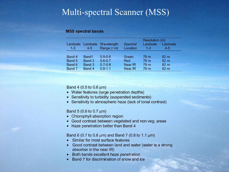
Multi-spectral Scanner (MSS)

IFOV at nadir 79 x 79 m for bands 4 to 7

240 x 240 m for band 8

Quantization levels 6 bit (values from 0 to 63) in 1970’s

8 bit (values from 0 to 255) in 1980’s

Earth coverage 18 days Landsat 1,2,3

16 days Landsat 4,5

Altitude 919 km

Swath width 185 km

Inclination 99°

Multi-spectral Scanner (MSS)

MSS Scanning Geometry

Multi-spectral Scanner (MSS)

Landsat 4 and 5 Thematic Mapper (TM)

IFOV at nadir 30 x 30 m for bands 1through 5, 7

120 x 120 m for band 6

Quantization levels 8 bit (values from 0 to 255)

Earth coverage 16 days Landsat 4,5

Altitude 705 km

Swath width 185 km

Inclination 98.2°

Landsat 4 and 5 Thematic Mapper (TM)

Landsat 4 and 5 Thematic Mapper (TM)

Enhanced Thematic Mapper Plus (ETM+)

IFOV at nadir 30 x 30 m for bands 1through 5, 7

60 x 60 m for band 6

15 x 15 m for band 8 (panchromatic)

Quantization levels 8 bit (values from 0 to 255)

Revisit 16 days

Altitude 705 km

Swath width 185 km

Inclination 98.2°

Enhanced Thematic Mapper Plus (ETM+)

Spatial and Spectral Resolution of Landsat

Multi-spectral Scanner (MSS), Thematic Mapper (TM),

and Enhanced Thematic Mapper Plus (ETM+)

Multi-spectral Scanner (MSS), Thematic Mapper (TM),

and Enhanced Thematic Mapper Plus (ETM+)

Jensen, 2007

Landsat Path and Row

• Orbit paths are numbered westward, with path 001 passing through Eastern Greenland and South America

• Image rows are numbered southward beginning at 80 deg. N. Latitude, and with row 60 being closest to the equator

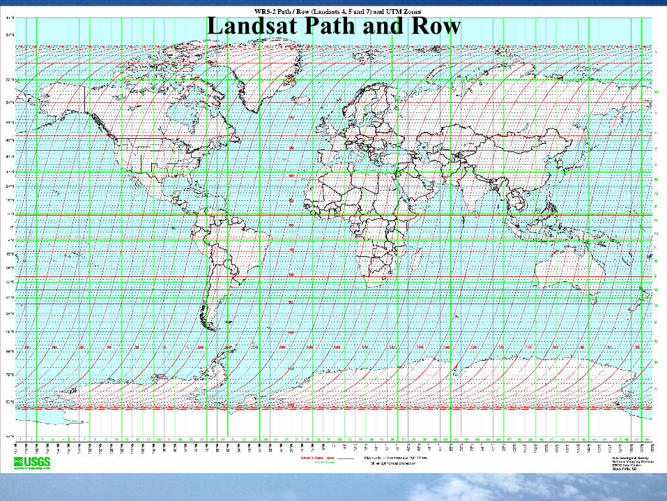
Landsat Path and Row

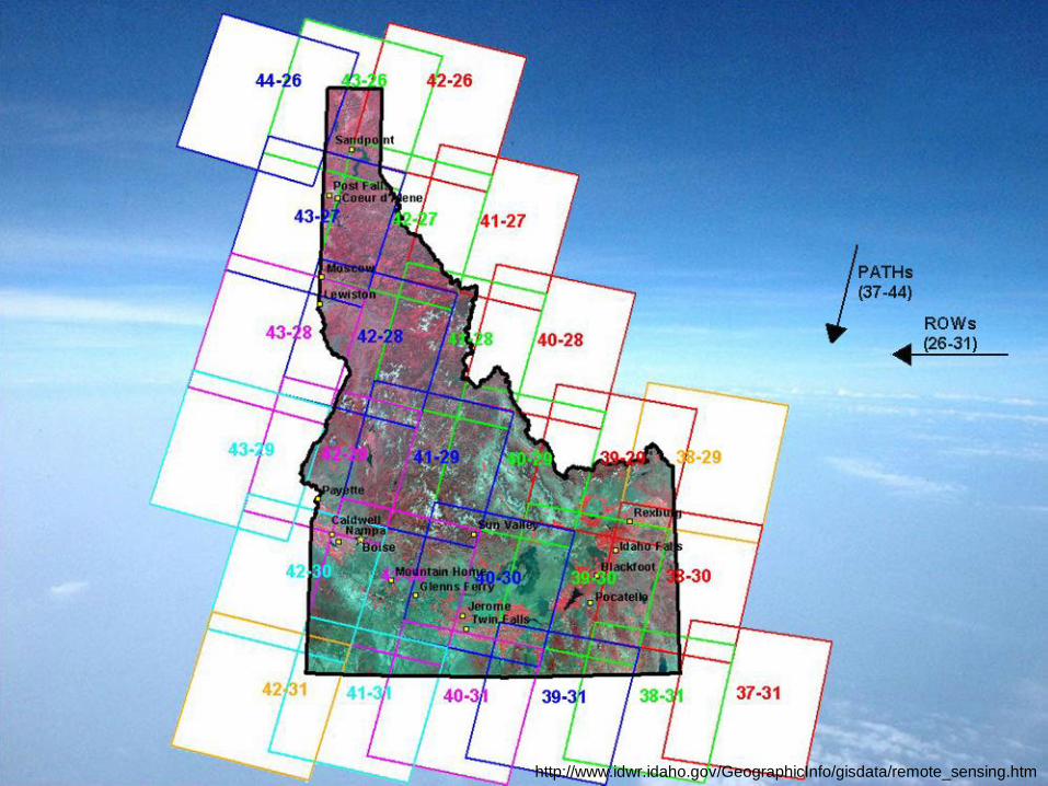
http://www.idwr.idaho.gov/GeographicInfo/gisdata/remote_sensing.htm

Landsat Path and Row

http://glovis.usgs.gov/

Landsat Data Availability

• All data available through EROS Data Center (EDC); partnership w/USGS

• Prices Prior to 2009:

– ETM+ ~$600/scene ($250 each additional scene)

– TM ~$400/scene ($200 each additional scene)

– MSS ~$200/scene ($100 each additional scene)

• Since 2009, global data sets have been made available free of charge from Landsats 4, 5, and 7, TM.

The 1973

Mount St. Helens

http://eros.usgs.gov/

The 1983

Mount St. Helens

http://eros.usgs.gov/

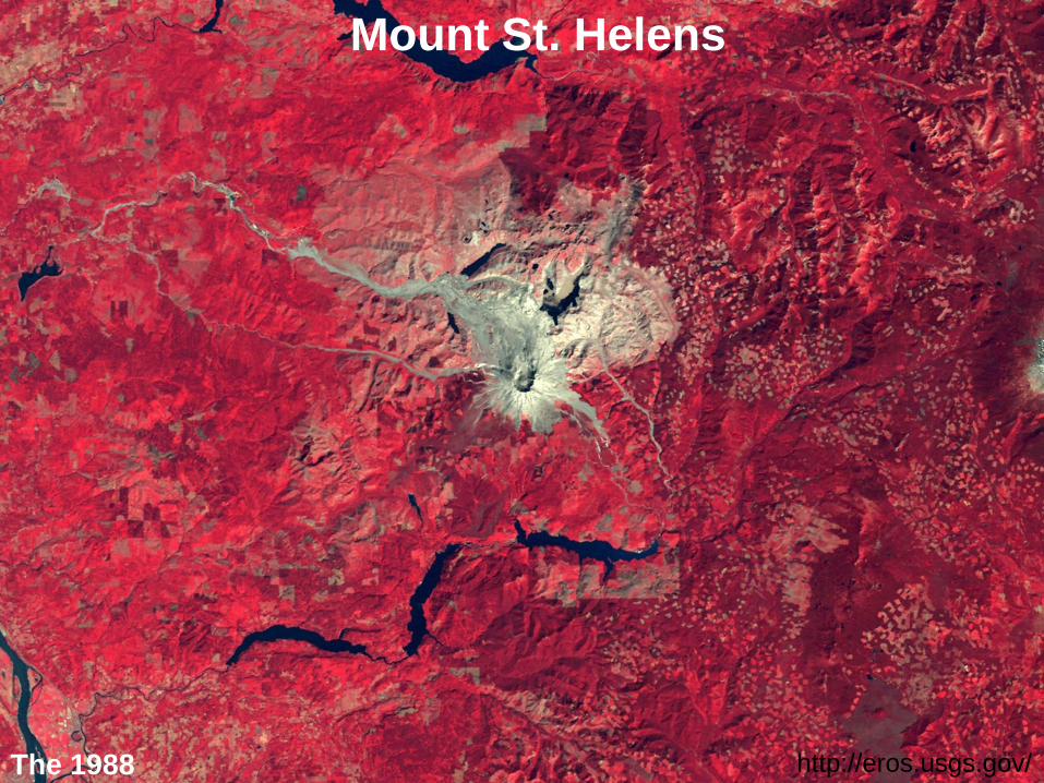
The 1988

Mount St. Helens

http://eros.usgs.gov/

The 1992

Mount St. Helens

http://eros.usgs.gov/

Mount St. Helens: Thirty Years Later

NASA Goddard space flight center