While there is a generally While there is a generally accepted precise definition accepted precise definition for the term "first order for the term "first order differential equation'', this differential equation'', this is not the case for the term is not the case for the term "Bifurcation''. View "Bifurcation''. View "bifurcation" as a "bifurcation" as a description of certain description of certain phenomena insteadphenomena instead..

In a very crude way, we will say In a very crude way, we will say that a system undergoes a that a system undergoes a bifurcation if and only if the global bifurcation if and only if the global behavior of a system, which behavior of a system, which depends on a parameter, changes depends on a parameter, changes when the parameter varies. Let us when the parameter varies. Let us illustrate this through the illustrate this through the population dynamics example. population dynamics example. Indeed, consider the logistic Indeed, consider the logistic equation describing a certain fish equation describing a certain fish

populationpopulation )1( ppdt

dp

where where PP((tt) is the population of the ) is the population of the fish at time fish at time tt. If we assume that . If we assume that the fish are harvested at a the fish are harvested at a constant rate (for example), then constant rate (for example), then we have to modify the differential we have to modify the differential

equation toequation to

Hppdt

dp )1(

where where HH > 0 is the constant harvesting > 0 is the constant harvesting rate. Here is a simple example of a real-rate. Here is a simple example of a real-world problem modeled by a differential world problem modeled by a differential equation involving a parameter (the equation involving a parameter (the constant rate constant rate HH). Clearly, the fishermen ). Clearly, the fishermen will be happy if will be happy if HH is big, while ecologists is big, while ecologists will argue for a smaller will argue for a smaller HH (in order to (in order to protect the fish population). What then protect the fish population). What then is the ``optimal'' constant is the ``optimal'' constant HH (if such (if such constant exists) which allows maximal constant exists) which allows maximal harvesting without endangering the harvesting without endangering the

survival of the fish populationsurvival of the fish population??

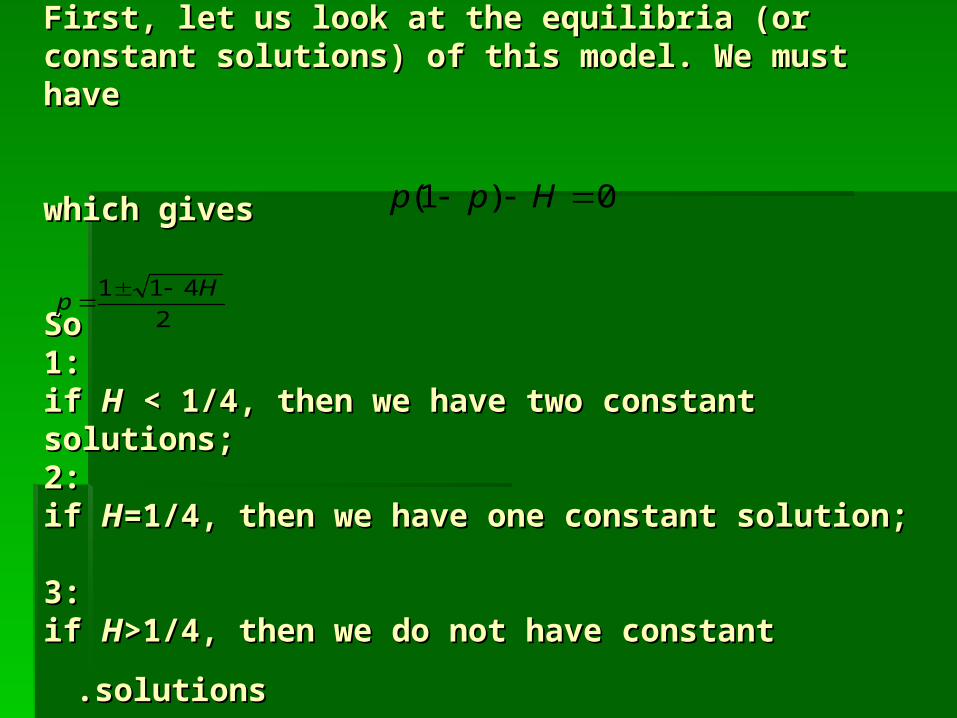
First, let us look at the equilibria (or constant First, let us look at the equilibria (or constant solutions) of this model. We must have solutions) of this model. We must have

which gives which gives

SoSo1:1:if if HH < 1/4, then we have two constant solutions; < 1/4, then we have two constant solutions;

2: 2: if if HH=1/4, then we have one constant solution; =1/4, then we have one constant solution; 3: 3: if if HH>1/4, then we do not have constant >1/4, then we do not have constant

solutionssolutions..

0)1( Hpp

2

411 Hp

This is an example of what is This is an example of what is meant by "bifurcation". As you meant by "bifurcation". As you see the number of equilibria (or see the number of equilibria (or constant solutions) changes constant solutions) changes (from two to zero) as the (from two to zero) as the parameter parameter HH changes (from changes (from below 1/4 to above 1/4). Note below 1/4 to above 1/4). Note that this is just one form of that this is just one form of bifurcation; there are other bifurcation; there are other forms or changes, which are forms or changes, which are

also called bifurcationsalso called bifurcations

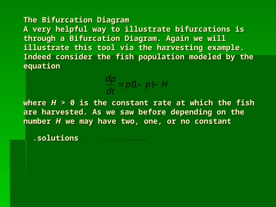
The Bifurcation DiagramThe Bifurcation DiagramA very helpful way to illustrate bifurcations is through A very helpful way to illustrate bifurcations is through a Bifurcation Diagram. Again we will illustrate this tool a Bifurcation Diagram. Again we will illustrate this tool via the harvesting example. Indeed consider the fish via the harvesting example. Indeed consider the fish population modeled by the equation population modeled by the equation

where where HH > 0 is the constant rate at which the fish are > 0 is the constant rate at which the fish are harvested. As we saw before depending on the number harvested. As we saw before depending on the number

HH we may have two, one, or no constant solutions we may have two, one, or no constant solutions..

Hppdt

dp )1(

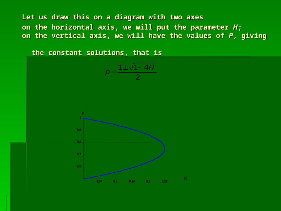
Let us draw this on a diagram with two axes Let us draw this on a diagram with two axes

on the horizontal axis, we will put the parameter on the horizontal axis, we will put the parameter HH; ; on the vertical axis, we will have the values of on the vertical axis, we will have the values of PP, giving the , giving the

constant solutions, that isconstant solutions, that is

2

411 Hp

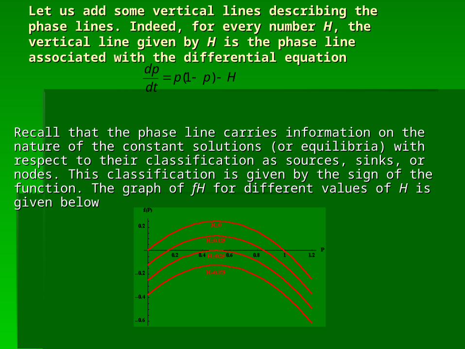
Let us add some vertical lines describing the phase Let us add some vertical lines describing the phase lines. Indeed, for every number lines. Indeed, for every number HH, the vertical line , the vertical line given by given by HH is the phase line associated with the is the phase line associated with the differential equationdifferential equation

Recall that the phase line carries information on the nature of the constant Recall that the phase line carries information on the nature of the constant solutions (or equilibria) with respect to their classification as sources, sinks, solutions (or equilibria) with respect to their classification as sources, sinks, or nodes. This classification is given by the sign of the function. The graph or nodes. This classification is given by the sign of the function. The graph of of fHfH for different values of for different values of HH is given below is given below

Hppdt

dp )1(

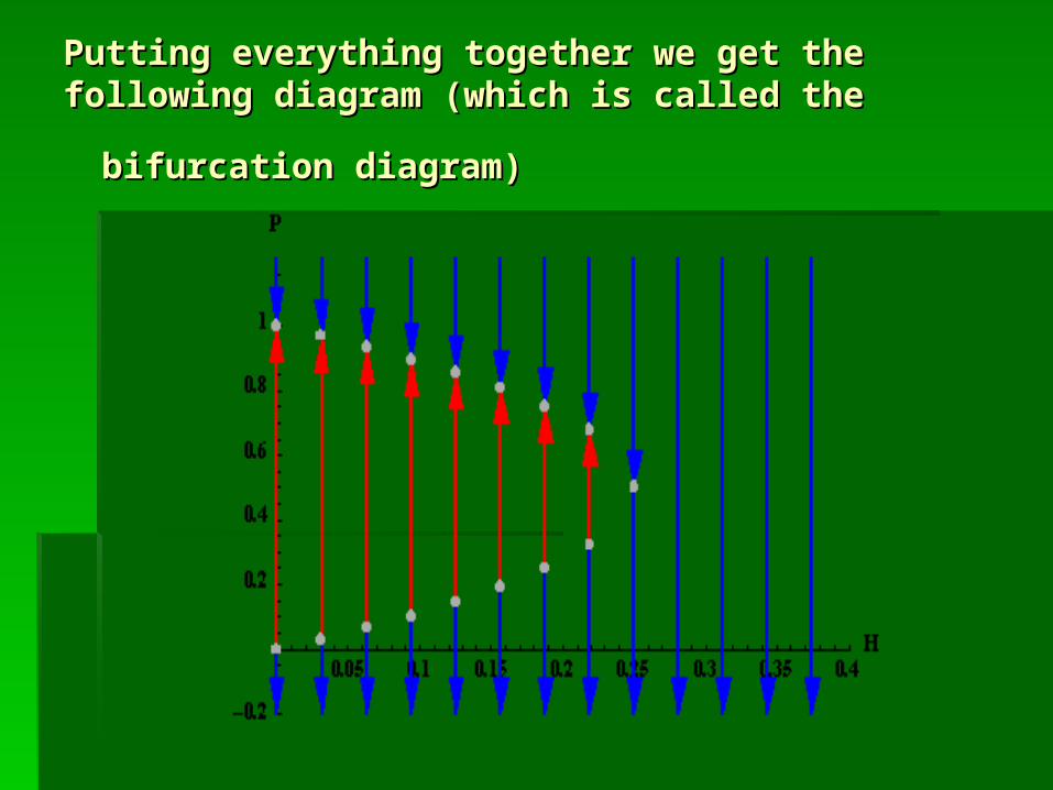
Putting everything together we get the Putting everything together we get the following diagram (which is called the following diagram (which is called the

bifurcation diagram)bifurcation diagram)

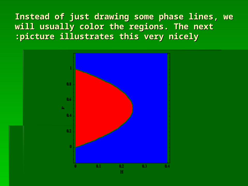
Instead of just drawing some phase lines, we Instead of just drawing some phase lines, we will usually color the regions. The next picture will usually color the regions. The next picture illustrates this very nicelyillustrates this very nicely::

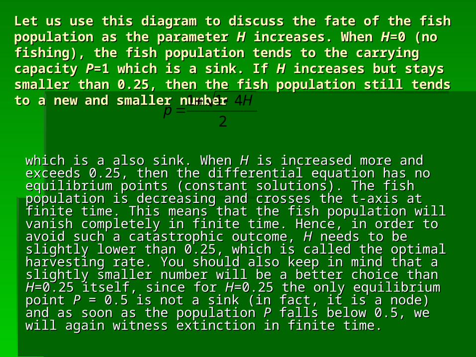
Let us use this diagram to discuss the fate of the fish Let us use this diagram to discuss the fate of the fish population as the parameter population as the parameter HH increases. When increases. When HH=0 (no =0 (no fishing), the fish population tends to the carrying capacity fishing), the fish population tends to the carrying capacity PP=1 which is a sink. If =1 which is a sink. If HH increases but stays smaller than increases but stays smaller than 0.25, then the fish population still tends to a new0.25, then the fish population still tends to a new and and smaller numbersmaller number

which is a also sink. When which is a also sink. When HH is increased more and exceeds is increased more and exceeds 0.25, then the differential equation has no equilibrium points 0.25, then the differential equation has no equilibrium points (constant solutions). The fish population is decreasing and (constant solutions). The fish population is decreasing and crosses the t-axis at finite time. This means that the fish crosses the t-axis at finite time. This means that the fish population will vanish completely in finite time. Hence, in order population will vanish completely in finite time. Hence, in order to avoid such a catastrophic outcome, to avoid such a catastrophic outcome, HH needs to be slightly needs to be slightly lower than 0.25, which is called the optimal harvesting rate. You lower than 0.25, which is called the optimal harvesting rate. You should also keep in mind that a slightly smaller number will be a should also keep in mind that a slightly smaller number will be a better choice than better choice than HH=0.25 itself, since for =0.25 itself, since for HH=0.25 the only =0.25 the only equilibrium point equilibrium point PP = 0.5 is not a sink (in fact, it is a node) and = 0.5 is not a sink (in fact, it is a node) and as soon as the population as soon as the population PP falls below 0.5, we will again witness falls below 0.5, we will again witness extinction in finite time.extinction in finite time.

2

411 Hp

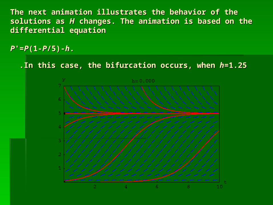
The next animation illustrates the behavior of the The next animation illustrates the behavior of the solutions as solutions as HH changes. The animation is based on the changes. The animation is based on the differential equation differential equation

PP'='=PP(1-(1-PP/5)-/5)-hh..

In this case, the bifurcation occurs, when In this case, the bifurcation occurs, when hh=1.25=1.25..

Example: Consider the autonomous equation Example: Consider the autonomous equation

with parameter with parameter aa. . 1.Draw the bifurcation diagram for this differential 1.Draw the bifurcation diagram for this differential equation.equation. 2.Find the bifurcation values and describe how the 2.Find the bifurcation values and describe how the behavior of the solutions changes close to each behavior of the solutions changes close to each bifurcation value. bifurcation value.

Solution:Solution: First, we need to find the equilibrium points (critical First, we need to find the equilibrium points (critical points). They are found by setting . We get points). They are found by setting . We get This a quadratic equation which solves intoThis a quadratic equation which solves into

42 ayydt

dy

0dt

dy.042 ayy

442

2

aa

y

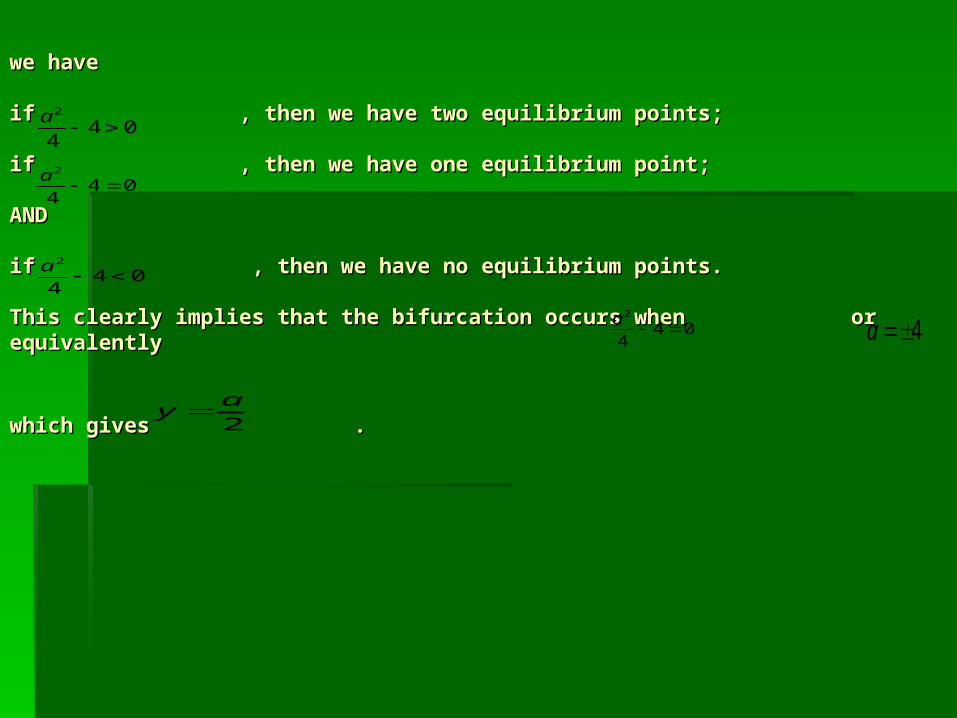
we havewe have if , then we have two equilibrium points; if , then we have two equilibrium points;

if , then we have one equilibrium point; if , then we have one equilibrium point;

ANDAND if , then we have no equilibrium points. if , then we have no equilibrium points.

This clearly implies that the bifurcation occurs when or This clearly implies that the bifurcation occurs when or equivalently equivalently

which gives .which gives .

044

2

a

044

2

a

044

2

a

4a

2

ay

044

2

a

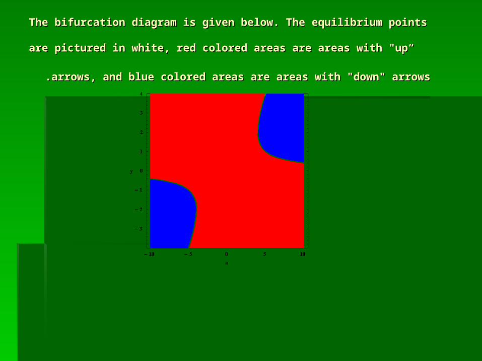
The bifurcation diagram is given below. The equilibrium points The bifurcation diagram is given below. The equilibrium points

are pictured in white, red colored areas are areas with "up“ arrows, are pictured in white, red colored areas are areas with "up“ arrows,

and blue colored areas are areas with "down" arrowsand blue colored areas are areas with "down" arrows..

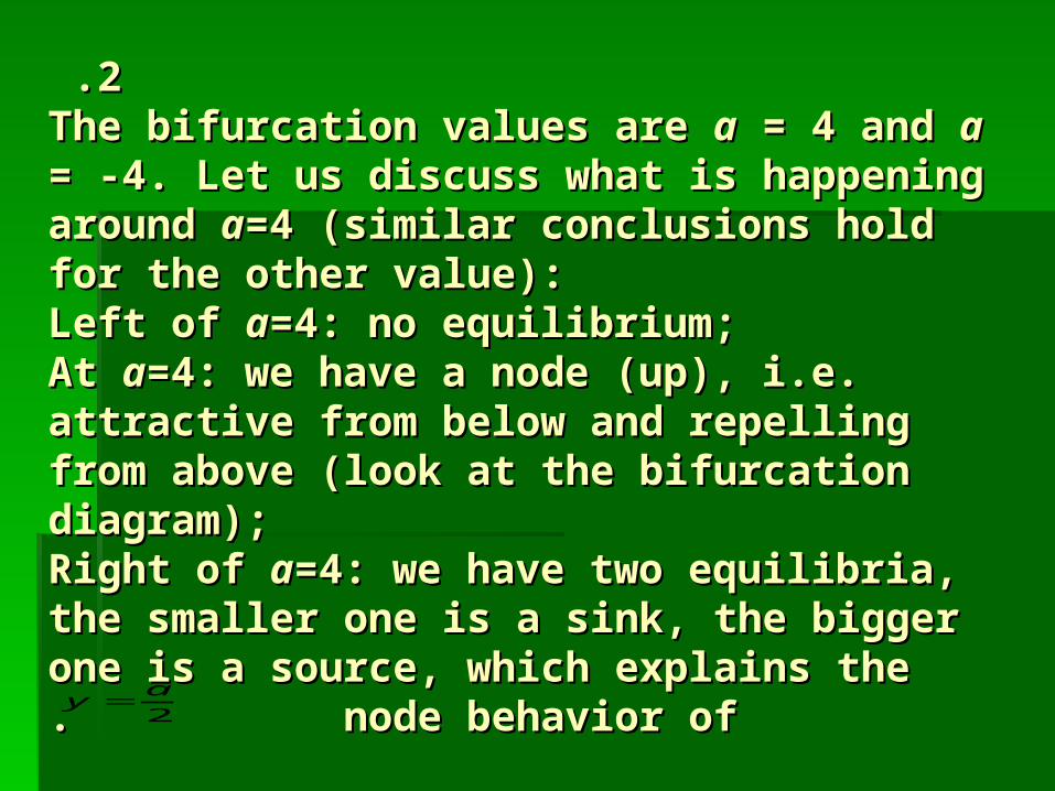
22 . .The bifurcation values are The bifurcation values are aa = 4 and = 4 and aa = - = -4. Let us discuss what is happening 4. Let us discuss what is happening around around aa=4 (similar conclusions hold for =4 (similar conclusions hold for the other value): the other value): Left of Left of aa=4: no equilibrium; =4: no equilibrium; At At aa=4: we have a node (up), i.e. =4: we have a node (up), i.e. attractive from below and repelling from attractive from below and repelling from above (look at the bifurcation diagram); above (look at the bifurcation diagram); Right of Right of aa=4: we have two equilibria, the =4: we have two equilibria, the smaller one is a sink, the bigger one is a smaller one is a sink, the bigger one is a source, which explains the node source, which explains the node

behavior ofbehavior of. . 2

ay