Which Sums of Squares Are Best in Unbalanced Analysis · PDF fileWhich Sums of Squares Are...

Which Sums of Squares Are BestIn Unbalanced Analysis of Variance?

Donald B. Macnaughton*

Note added on May 10, 1998: A few months after I originally published this paper I discovered a particular (infrequentlyoccurring) situation in which the recommended HTO approach to unbalanced analysis of variance is invalid. (The HTOSapproach, which I recommend in appendix D as an extension of the HTO approach, is valid in this situation.) I shall dis-cuss this matter in a forthcoming paper.

Three fundamental concepts of science and statistics areentities, variables (which are formal representations ofproperties of entities), and relationships between vari-ables. These concepts help to distinguish between twouses of the statistical tests in analysis of variance(ANOVA), namely• to test for relationships between the response variable

and the predictor variables in an experiment• to test for relationships among the parameters of the

model equation in an experiment.Two methods of computing ANOVA sums of squares are:• Higher-level Terms are Omitted from the generating

model equations (HTO = SPSS ANOVA EXPERIMEN-TAL ≈ SAS Type II ≈ BMDP4V with Weights are Sizes)

• Higher-level Terms are Included in the generating modelequations (HTI = SPSS ANOVA UNIQUE = SPSSMANOVA UNIQUE = SAS Type III = BMDP4V withWeights are Equal = BMDP2V = MINITAB GLM =SYSTAT MGLH = Data Desk Type 3).

This paper evaluates the HTO and HTI methods of com-puting ANOVA sums for squares for fulfilling the twouses of the ANOVA statistical tests. Evaluation is interms of the hypotheses being tested and relative power.It is concluded that (contrary to current practice) the HTOmethod is generally preferable when a researcher wishesto test the results of an experiment for evidence of rela-tionships between variables.

KEY WORDS: Relationships between variables; Rela-tionships among parameters; Philosophy of ANOVA;Power of ANOVA.

1. INTRODUCTIONMethods of computing analysis of variance (ANOVA)

sums of squares for unbalanced experiments were intro-duced by Yates in 1934. Recently there has been contro-versy over which method is “best”. This expository paper

addresses some areas of the controversy.Section 2 gives references to earlier work. Sections 3

- 6 discuss preparatory topics. Sections 7 - 11 describetwo uses of the ANOVA statistical tests. Sections 12 and13 describe two methods of computing ANOVA sums ofsquares. Sections 14 - 18 evaluate the two methods forfulfilling the two uses. Five appendices extend the ideas.

I hope that knowledgeable readers will indulge myinitial concentration (in sections 3 - 6) on some fundamen-tal concepts of human thought. These concepts may atfirst seem trivial or obvious. However, these concepts de-serve careful study because they are foundations for manyother concepts in science and statistics, including theconclusions of this paper.

Most of the discussion that follows is non-mathemati-cal. However, readers who enjoy a mathematical cres-cendo may get some satisfaction from the elegant sim-plicity of works of three statisticians excerpted in appen-dix C.

2. HISTORYReaders wishing to trace the development of ideas

about unbalanced ANOVA will find the works by thefollowing authors of interest (given here in chronologicalorder): Yates (1934), Kempthorne (1952), Scheffé(1959:112-119), Elston and Bush (1964), Gosslee and Lu-cas (1965), Bancroft (1968), Overall and Spiegel (1969),Speed (1969), Francis (1973), Urquhart, Weeks, andHenderson (1973), Appelbaum and Cramer (1974),Burdick, Herr, O’Fallon, and O’Neill (1974), Carlson andTimm (1974), Kutner (1974), Kutner (1975), Hocking andSpeed (1975), Overall, Spiegel, and Cohen (1975), Golharand Skillings (1976), Hocking and Speed (1976), Kerenand Lewis (1976), O’Brien (1976), Speed and Hocking(1976), Heiberger and Laster (1977), Nelder (1977), Ait-kin (1978), Herr and Gaebelein (1978), Hocking, Hack-ney, and Speed (1978), Speed, Hocking, and Hackney(1978), Urquhart and Weeks (1978), Burdick (1979),Frane (1979), Bryce, Scott, and Carter (1980), Burdickand Herr (1980), Cramer and Appelbaum (1980), Good-night (1980), Hocking, Speed, and Coleman (1980),Searle (1980), Steinhorst and Everson (1980), Overall,Lee, and Hornick (1981), Rubin, Stroud, and Thayer(1981), Searle (1981), Searle, Speed, and Henderson

*Donald B. Macnaughton is president of MatStat Research ConsultingInc. 246 Cortleigh Blvd., Toronto Ontario, Canada M5N 1P7. Email:[email protected] This article is a revised version of a paper pre-sented at the Joint Statistical Meetings in Boston, August 1992. Theauthor thanks Donald S. Burdick for the proof of theorem 2, and DonaldS. Burdick, Donald F. Burrill, Ramon C. Littell, and Jacqueline Oler forhelpful comments.

Sums of Squares in Unbalanced ANOVA 2.

(1981), Spector, Voissem, and Cone (1981), Calinski(1982), Howell and McConaughy (1982), Nelder (1982),Steinhorst (1982), Aitkin (1983), Littell and Lynch (1983),Schmoyer (1984), Johnson and Herr (1984), Hocking(1985), Elliott and Woodward (1986), Pendleton, VonTress, and Bremer (1986), Finney (1987), Knoke (1987),Milligan, Wong, and Thompson (1987), Searle (1987),Helms (1988), Singh and Singh (1989), Turner (1990),and Macdonald (1991). An excellent overview and fur-ther early references are given by Herr (1986).

3. ENTITIESIf you observe your train of thought, you will prob-

ably agree that you think about various “things”. For ex-ample, during the next few moments you might thinkabout, among other things, a friend, an appointment, to-day’s weather, and an idea. Each of these things is an ex-ample of an entity.

The concept of entity is perhaps the broadest of allhuman concepts, because literally everything (whether itexists or not) is an instance of an entity. Table 1 illus-trates the broadness by listing a variety of entity types.

cussions usually concern one or more types of entities,which are best referred to by their type names. (For ex-ample, medical scientists often study a of type of entitycalled human beings.) Or discussions may refer to one ormore individual entities, which are best referred to bytheir individual names. However, it is useful to be awareof the central role that the concept of entity plays in hu-man thought.

4. PROPERTIES OF ENTITIESAssociated with every entity are attributes or proper-

ties. Table 2 lists some entity types and some of the prop-erties associated with entities of each type.

TABLE 2

Entity Types with Examples ofSome of Their Properties

Entity Type Properties of Entities of this Type

physical objects weightchemical compositionage

persons heightintelligence quotientblood typepolitical affiliationwhether presently alive

forces magnitudedirectionlocus of application

national economies gross national productcost of livingrate of inflation

populations sizeproportion of the population

having a specified level of a property

events probability of occurrencewhether occurredduration

works of art beauty

TABLE 1

A List of Some Common Entity Types(some categories overlap)

physical objects (examples: trees, automobiles, protons)

processes (examples: a leaf blowing in the wind, a ma-chine building another machine, a chemical reaction)

events

organisms

minds

symbols

forces (examples: force needed to lift a physical object,magnetic forces)

mathematical entities (examples: sets, functions, num-bers, spaces, vectors)

relationships between entities

properties of entities

Most people view most entities as existing in two dif-ferent places: in the external world and in our minds. Weuse the entities in our minds mainly to stand for the enti-ties in the external world. This helps us to understand theexternal world. In language we represent entities withnouns.

The concept of entity does not often appear in scien-tific or statistical discussions because it is not often neces-sary to discuss things at such a general level. Instead, dis-

Properties are an important aspect of entities becausewe can only know or experience an entity by knowing orexperiencing its properties.

Kendall, Stuart, and Ord (1987:1.1-1.3) discuss therole of properties in statistics.

5. VALUES OF PROPERTIES OF ENTITIESFor any particular entity, each of its properties has a


value. People usually report the value of a property of anentity by one or more words or by a number. For exam-ple, table 3 lists some of the properties and the associatedvalues for the entity known as the United Nations Build-ing in New York City.

And the intersection of a row and a column contains thevalue of the property associated with the column for theparticular entity that is associated with the row.

• The concepts of entities and properties appear directly inknowledge representation in artificial intelligence(expert) systems where they are sometimes organizedinto “semantic networks” or “frames”.

• Entities and properties appear in object-oriented pro-gramming languages in the sense that the objects andattributes (variables) of such languages are simply enti-ties (or sometimes classes of entities) and properties re-spectively.

6. RELATIONSHIPS BETWEEN PROPERTIES(RELATIONSHIPS BETWEEN VARIABLES)

6.1 Science as a Study of Relationships Between Prop-erties

In view of the broad generality of the concepts ofentities and properties, it is helpful to consider scientificresearch in terms of those concepts. In those terms, muchof science can be seen as a study of relationships betweenproperties of entities.

One can characterize a relationship between proper-ties as follows:

There is a relationship in entities between a propertyy and one or more other properties x1, x2, ..., xp if anyof the following (equivalent) conditions are satisfied:• the measured value of y in the entities “depends” on

the measured values of the x’s in the entities or• the measured value of y in the entities varies wholly

or partially “in step” with the measured values ofthe x’s in the entities or

• y is some function of the x’s in the entities—that is

y f x x xp= +( , , , )1 2 K e (1)

(where I discuss the term e below).

For example, medical scientists have discovered thatthere is a relationship in humans between the property“concentration of insulin in the bloodstream” and theproperty “rate of carbohydrate metabolism”. Specifically,as insulin in the bloodstream increases (within a certainrange), carbohydrate metabolism also increases.

Scientists often summarize their findings of a rela-tionship between properties with a graph, such as figure 1.

We can see the generality of the concept of arelationship between properties of entities if we examinethe so-called laws of science, and if we note that many ofthese laws are statements of relationships between proper-ties of entities. For example, the ideal gas law, PV = nRT,that relates pressure (P), volume (V), amount (n), andtemperature (T) of an ideal gas is a statement of a relation-ship between certain properties of a mass of gas. (The Ris the constant of proportionality.)

TABLE 3

Properties of the United Nations Buildingand Their Associated Values

Property Value of the Property

height tall (i.e., the word tall)

height in meters 165.8

primary building materials concrete, glass, steel

In language we often use adjectives and adverbs toreport the values of properties. For example, we mightuse the adjective tall to report (the value of) the height(property) of a building, or the adverb quickly to report(the value of) the speed (property) of (the process of)someone running in a race.

Adjectives and adverbs are useful for reporting thevalues of properties because they are compact—within asingle word we can both identify the property of interestand indicate a particular value of it. However, adjectivesand adverbs are also imprecise. If we need higher preci-sion in the report of the value of a property, we can usenumbers because numbers can represent any degree ofprecision we wish.

If we wish to determine the value of a property of anentity, we can apply an appropriate measuring instrumentto the entity. If the instrument is measuring correctly, itwill return a value to us that is an estimate of the value ofthe property in the entity at the time of the measurement.

References to values of properties of entities are sucha fundamental part of people’s thinking that we usuallymake these references automatically, without being spe-cifically aware that we are using the general concept of avalue of a property of an entity. Therefore, the impor-tance of values of properties of entities in models of theexternal world may be sometimes underestimated.

Computer models of the external world are playingincreasingly important roles in science, business, and gov-ernment. Therefore, it is interesting to note the centralroles that entities, properties, and values play in suchmodels:• Each table in a computer database is associated with a

different type of entity about which the user of the data-base wishes to keep information. For any given table,the rows of the table represent different instances of en-tities of the type associated with the table. The columnsrepresent different properties of entities of this type.


TABLE 4

Classification of “Laws” Defined inDictionary of Scientific Terms

Type of Statement % Count*

relationship between properties 75 184

non-relationship between properties(including 10 conservation laws)

11 27

law of mathematics(axiom or theorem)

6 14

relationship between entities 4 9

value of a property 2 5

distribution of the values of a property 2 4

existence of a property 1 2

existence of an entity <1 1

other 0 0

*The sum of the counts is greater than 213 because some laws containedtwo or more independent statements, and each such statement was classi-fied separately. For some laws, instances of the one or more statementsthat constitute the law could sometimes, by taking different points of view,be classified in more than one of the first eight ways. In those cases, thecount reflects the way of classifying the statement that was judged easiestto understand.

0

3

6

9

0 50 100 150

Insulin Concentration in mU/ml

GlucoseUptake Rate

in mg/(kg-min)

Figure 1. A graph showing the relationship between carbohy-drate metabolism (specifically glucose uptake) and insulin con-centration for fifteen normal young adults. Data are from anexperiment by Gottesman et al (1982). The height of each blacksquare indicates the mean glucose uptake when the subjectswere maintained at the insulin concentration shown on the hori-zontal axis directly beneath the square. (Plasma glucose wasmaintained at approximately 92 mg/dl throughout.) The hori-zontal bars show plus and minus the standard error of each glu-cose uptake mean.

Similarly, Einstein’s equation, E = mc2 is a statementof a relationship between two properties of matter: con-tained energy (E) and mass (m). (The c2 is the constant ofproportionality, which Einstein has shown to be equal tothe square of the speed of light.)

To explore the generality of the concept of a relation-ship between properties, two assistants each scanned eachpage of the 2088-page McGraw-Hill Dictionary of Scien-tific and Technical Terms (Parker 1989) for entries thatcontain the word law in the definiendum. They found213 entries that define different “laws” of science. Foreach entry I then tried to express the definition in terms ofthe concepts of entities, properties, and relationships be-tween properties. This yielded the classification shown intable 4.

The most common type of statement in science—astatement of a relationship between properties—is also themost important because knowledge of relationships be-tween properties gives us the ability to predict (and some-times control) the values of properties in new similar enti-ties, and such ability is often of great value. For example,knowledge of the relationship between “concentration ofinsulin in the bloodstream” and “rate of carbohydrate me-tabolism” in humans has helped doctors to control diabe-tes, a disease that is characterized by poor carbohydratemetabolism.

Summarizing: Study of relationships between prop-

erties of entities is a central activity of science becauseknowledge of such relationships gives us the ability topredict and control (values of) properties, and such abilityis often of great value.

6.2 Properties as VariablesBypassing some details (see Macnaughton 1997), we

can roughly say that scientists and statisticians usually re-fer to properties as variables. Much of statistics is aimedat providing techniques to help scientists study relation-ships between variables, whether through the t-test,ANOVA, regression, exploratory data analysis, nonpara-metric analysis, categorical analysis, time series analysis,survey analysis, factor analysis, correspondence analysis,or various other techniques.

In the rest of the paper I use standard terminology anddiscuss properties and relationships between propertiesmainly in terms of variables and relationships betweenvariables. However, readers new to the ideas may find ithelpful to keep in mind that the variables that are dis-cussed in science are simply representations of propertiesof entities. And the value of any variable represents thevalue of the property in the associated entity (usually at aparticular time).


(In the physical sciences, properties, variables, or val-ues are sometimes called physical quantities.)

Barnett (1988) gives a general discussion of the con-cept of a relationship between variables.

6.3 Response Variables and Predictor VariablesIn studying relationships between variables, scientists

often classify the variables in a research project into re-sponse variables and predictor variables. The responsevariables are the variables that the scientist would like todiscover how to control (or at least predict). The predic-tor variables are the variables that the scientist will control(or just measure) in an attempt to discover how to control(predict) the values of the response variables.

For example, when medical scientists study the rela-tionship between “concentration of insulin in the blood-stream” and “rate of carbohydrate metabolism”, they view“rate of carbohydrate metabolism” as the response vari-able because they wish to learn how to control carbohy-drate metabolism by controlling insulin concentration (andnot the other way around).

Most scientists find it efficient to concentrate onlearning how to control or predict a single variable at atime in the entities they are studying. Therefore, withoutloss of relevant generality, this paper discusses researchprojects (or standalone units of analysis in research pro-jects) that have a single response variable (which may bemeasured just once or repeatedly in entities) and one ormore predictor variables.

6.4 A Definition of a Relationship Between Properties(Variables)

The characterization of a relationship between prop-erties given in section 6.1 is statistically weak so, since weneed a statistical definition below, let us convert the char-acterization into such a definition. I begin with two pre-liminary definitions:

Definition: The expected value of a variable in apopulation is the average value of the variable acrossall the entities in the population under a given set ofconditions.

Definition: The expected value of a variable in apopulation conditioned on the values of one or moreother variables is the average value of the variableacross all the entities in the population under a givenset of conditions including the condition that the othervariables have particular stated values.

I shall represent the expected value of some variabley as E y( ) , and I shall represent the expected value of y

conditioned on the values of variables x xp1, ..., as

E y x xp( | ,..., ).1

Using the concept of expected value, let us now con-sider a formal definition of a relationship between proper-ties (variables):

Definition: If y is a variable that reflects a measuredproperty of entities in some population, and ifx xp1, ..., are a set of one or more other variables thatreflect distinct other measured properties of the enti-ties (or of the entities’ environment), then a relation-ship exists in the entities between y and the x xp1, ,Kif, for each integer i, where 1 £ £i p

E y x x x x x

E y x x x x

i i i p

i i p

( | ,..., , , ,..., )

( | ,..., , ,..., ).

1 1 1

1 1 1

- +

- +π

If p = 1, the inequality simplifies toE y x E y( | ) ( ).1 π

Each of the p inequalities is deemed to be satisfied ifthere is at least one set of specific values of the xs thatsatisfies the inequality. (Notes: (1) A different set ofvalues of the xs may be used for each inequality; (2)if y is not a numeric variable, then for a relationshipto exist, the p inequalities must each be satisfied forat least one recoding of the values of y into numericvalues. A different recoding may be used for each in-equality.)

Note that this definition of a relationship betweenproperties is operationally equivalent to the characteriza-tions of a relationship given in section 6.1 because if astate of affairs satisfies the definition, it will also satisfyany of the characterizations, and vice versa.

Other mathematical definitions of a relationship be-tween properties are given (in terms of causal relation-ships) by Granger (1980), Chowdhury (1987), and Poirier(1988).

6.5 The Null and Alternative HypothesesFor any type of entity and any response variable and

any set of one or more predictor variables, exactly one ofthe following two hypotheses is true:• Null Hypothesis: there is no relationship between the

response variable and any of the predictor variables inthe population of entities of this type

• Alternative Hypothesis: there is a relationship betweenthe response variable and one or more of the predictorvariables in the population.

Scientists usually begin study of a relationship be-tween variables with the formal assumption that null hy-pothesis is true. (Informally we usually suspect and hopethat the alternative hypothesis is true or there would be nopoint in seeking evidence of relationships in the particularset of variables we are studying.) The practice of begin-ning with the (impossible-to-prove) assumption that thenull hypothesis is true is entailed by the principle of par-simony, which tells us to keep things as simple as possi-


ble. The simplest situation is that of no relationship, sowe begin with that assumption.

After making the assumption that the null hypothesisis true, scientists who wish to study a relationship thenperform an appropriate research project in an attempt toinvalidate the assumption. If the results of the researchproject show reasonable evidence that a relationship ex-ists, then the scientific community (through informal con-sensus) rejects the null hypothesis and concludes that arelationship between variables similar to that suggested bythe results probably actually exists.

Tukey (1989:176) suggests that there may be a rela-tionship (albeit sometimes very weak) in entities betweenall measurable pairs of variables, regardless of the vari-ables’ identities. Given that point, we may ask why it isnecessary to begin with the assumption that the null hy-pothesis is true. Researchers begin initial study of a rela-tionship between variables with the (formal) assumptionthat there is no relationship in order to avoid the problemof thinking that they know more about a relationship thanthey actually do. And only if all of the following condi-tions are satisfied do careful researchers accept the exis-tence of a particular relationship between variables:• someone has performed an appropriate empirical re-

search project• the research project has found reasonable (see below)

evidence of a relationship between the variables• the research project has been carefully scrutinized for er-

rors (and perhaps replicated) by the scientific commu-nity (and anyone else who is interested)

• nobody has been able to come up with a reasonable al-ternative explanation of the results of the research pro-ject (see Mosteller 1990, Lipsey 1990, Macnaughton1997).

6.6 Experiments and CausationWhen scientists can control (“manipulate”) the values

of variables (as opposed to being able only to observethem), they usually study relationships between variablesby performing “experiments”.

Definition: An experiment consists of our manipulat-ing one or more predictor variables in one or moreentities while we observe a response variable in theentities.

Of course, we manipulate a variable in entities bysomehow causing the variable to have certain values ofour choosing in the entities. For example, in a medicalexperiment we can manipulate the concentration of insulinin the bloodstreams of patients by administering differingamounts of insulin to them.

When feasible, experiments are preferred to observa-tional (i.e., non-manipulative) research projects becauserelationships between variables found in experiments

usually allow us to infer causation while relationshipsbetween variables found in observational research projectsusually do not allow us to (confidently) infer causation—they only allow us to infer association.

This paper concentrates on analyzing the results ofexperiments. And although some of the points below alsoapply to non-experimental (i.e., observational) researchprojects, interpretation of such research projects is moredifficult, and beyond the present scope.

Landmark books about the design and analysis of ex-periments are by Fisher (1935 [1990]), Kempthorne(1952), Cochran and Cox (1957 [1992]), Cox (1958[1992]), Finney (1960), Winer (1971), and Box, Hunter,and Hunter (1978).

6.7 ANOVAIf certain often-satisfiable assumptions (discussed

below) are adequately satisfied, ANOVA is well suited toanalyze the results of an experiment to help determine ifthere is evidence of a relationship between the responsevariable and one or more of the predictor variables.

ANOVA works by taking as input the results of aproperly-carried-out experiment. That is, the input is the(ordered) set of values of the response and predictor vari-ables that were measured in the entities that participatedin the experiment. Through a mathematical procedure,ANOVA provides as its output a set of numbers called p-values. A p-value is:

the probability of obtaining the evidence(or stronger evidence)

available from the results of the experimentthat the particular type of relationship

(between the response variableand the predictor variables)

that is suggested by the resultsactually exists

if in fact there is no such relationship.Thus the lower a p-value, the more improbable it is

that the obtained result would be obtained if there is norelationship. Thus if a p-value for a relationship is lowenough, we can tentatively reject the null hypothesis andconclude that there is a relationship between the responsevariable and the relevant predictor variable(s).

In evaluating the work of others, scientists often usethe reasonable convention that a p-value must be less thana critical value of .05 (or sometimes .01) before they willreject the null hypothesis and tentatively conclude that therelationship that is associated with a p-value actually ex-ists.

The practice of computing a p-value and examining itto determine whether it is less than a critical value iscalled a statistical test of the hypothesis that the associ-ated relationship exists.

Once we have concluded (from a statistical test or


otherwise) that a particular relationship exists, we canthen use our knowledge of the relationship to help usmake predictions or exercise control.

6.8 Does ANOVA Detect Relationships Between Vari-ables?

Some readers may question whether we can view theuse of the statistical tests in ANOVA (or in its simplest in-carnation, the t-test) as a means for detecting relationshipsbetween variables. For example, consider a research pro-ject that uses a t-test to check if there evidence of a differ-ence between women and men in their response to somestandard form of medical treatment (as measured by somemedically acceptable measure of the response). Mostreaders will agree that a response variable is clearly pre-sent in this research project, namely the measured value ofthe “response” to the treatment for each person who par-ticipates in the research project. But some readers mayquestion whether there is a predictor variable, or whetherit is useful to view this research project in terms of seek-ing evidence of a relationship between variables.

We can answer these questions by first noting that thepredictor variable in the research project is the variable“gender”, which reflects an important property of the pa-tients. (“Gender” is a variable in the sense that for anypatient in the research project this variable has a particularvalue, namely, “female” or “male”, and the values varysomewhat from patient to patient.) Thus we can view theresearch project as an attempt to see if there is a relation-ship in humans between the variables “gender” and“response”.

Similarly, in an n-way ANOVA there are n differentpredictor variables, each of which represents a differentproperty of the entities that are under study, or of the enti-ties’ environment. (Of course, in the case of a treatmentthat is applied to the entities, the associated predictorvariable reflects a property of the entities after they havereceived the treatment. That is, the predictor variable re-flects the amount of the treatment—possibly zero—that anentity received.) Thus, as we shall see in more detail be-low, we can use ANOVA to help us determine whetherthere is evidence of a relationship between the responsevariable and one or more of the predictor variables in anexperiment.

But even if we agree that there are response and pre-dictor variables present in every ANOVA, the questionstill remains whether it is useful to view ANOVA as atechnique for detecting relationships between variables.To answer that question note that:• It is precisely instances of the concept of relationships

between variables in entities that most scientists are in-terested in detecting and describing when they useANOVA in research projects. That is, most scientistsare precisely interested in determining whether the ex-

pected value of some variable y depends on the values ofcertain other x-variables. They are interested in makingthis determination because if they find such a relation-ship, then we (as society) can confidently use theknowledge of the relationship to make predictions or toexercise control.

• As noted above, virtually all the statistical techniques asthey are used in empirical research can be viewed astechniques for studying (i.e., detecting and describing)relationships between variables. Viewing ANOVA andthe other techniques as techniques for studying relation-ships between variables helps to unify the techniques,and this unification facilitates understanding. The unifi-cation is especially helpful to newcomers to the field ofstatistics because it helps them to view the field in termsof an easy-to-understand and practical concept. (Thestatistical techniques for studying standalone distribu-tions are instances of the study of relationships betweenvariables in the sense that such techniques study rela-tionships between a response variable and a set ofpredictor variables when the set of predictor variables isempty. The techniques for studying relationships withnon-empty sets of predictor variables collapse neatlyinto this degenerate case.)

• Viewing ANOVA as a technique for studying relation-ships between variables helps to unravel certainimportant statistical problems, as we shall see later inthis paper.

6.9 Why We Need Statistical TestsOf course, we need not use a statistical test if we have

discovered a very strong relationship between variablesbecause in that case the results of the research project willusually leave no doubt as to the existence of the relation-ship. However, nowadays new strong relationships be-tween variables are not often discovered, perhaps becausemost of the strong relationships have already been discov-ered. Thus most relationships that are currently studiedare weak enough that statistical tests are necessary.

Recall Tukey’s (1989:176) suggestion that there maybe a relationship (albeit sometimes very weak) in entitiesbetween all measurable pairs of variables, regardless ofthe variables’ identities. Given that suggestion (and de-spite the arguments made in section 6.5 for beginning byassuming that the null hypothesis is true), we can still askwhy we need to use statistical tests to determine whetherthere is a evidence of a relationship between a particularpair of variables when, in fact, there almost surely is.

We need statistical tests because, as Tukey notes, inaddition to wishing to know with confidence whetherthere is a relationship between the variables, we usuallyneed information about the direction or profile of the re-lationship. (The profile tells us whether, when the valueof a given predictor variable increases in entities, the


value of the response variable can be expected to increaseor to decrease or perhaps to sometimes increase andsometimes decrease depending on the values of othervariables.) Only when we perform statistical tests can webe confident that the modest relationships between vari-ables that are typically suggested by the results of modernresearch accurately reflect profiles that we can expect tofind in similar entities in similar situations.

6.10 Interactions and Simple Relationships BetweenVariables

It is useful to classify relationships between variablesinto interactions and simple relationships:

Definition: If:• there is a relationship in entities between a re-

sponse variable y and p predictor variables x1, x2,..., xp where p ≥ 2 and

• the conditioning of y on the x’s cannot be repre-sented as a mathematical sum of separate simplerconditionings of y on one or more proper subsets ofthe same x’s and

• there is no higher-level interaction between the x1,x2, ..., xp and other predictor variables with respectto their joint relationship to y

we say the relationship is a p-way interaction betweenthe x1, x2, ..., xp with respect to their joint relationshipto y.

(The minor difficulty with the word interaction ap-pearing in the body of its own definition can be resolvedwith a more elaborate recursive definition, which I omithere for simplicity.)

Note that I have defined the concept of an interactionin terms of the more fundamental concept of a relationshipbetween variables. Interactions were invented by Fisher(1935, ch. VI) mainly as a means for detecting any formof relationship that might exist between the response vari-able and the predictor variables in a research project.

Definition: If:• there is a relationship in entities between a re-

sponse variable y and a single predictor variable x1

and• there is no evidence that there is an interaction

between x1 and any other predictor variable(s) with

respect to its relationship to ywe say the relationship is a simple relationship(sometimes called a main effect relationship).

The last bulleted paragraph in each of the precedingtwo definitions is usually not included in definitions ofinteraction and simple relationship. I discuss the useful-ness of these paragraphs in section 2 of appendix B.

6.11 Summary And PreviewIn sections 3 - 6 I discussed the concept of a relation-

ship between variables and I noted that one use of theANOVA statistical tests is to test for evidence of relation-ships between the response variable and the predictorvariable(s) in the population of entities that is studied inan experiment. In section 10 (after some preparatorywork in sections 7 - 9) I discusses a contrasting second useof the ANOVA statistical tests.

7. GROUP TREATMENT TABLESWe can summarize the layout of most experiments

with a group treatment table, as used extensively by Winer(1971). For example, table 5 summarizes a 2 ¥ 3 ex-periment in which two predictor variables, A and B, aremanipulated while we observe a response variable, y.

TABLE 5

Group Treatment Tablefor a 2 ¥ 3 Experiment

______________________

These Variables are ManipulatedBetween Groups of Entities Group______________

A B______________________

a0 b0 g1

a0 b1 g2

a0 b2 g3

a1 b0 g4

a1 b1 g5

a1 b2 g6______________________

Each of the g’s in the right side of the table representsa different “treatment group” of the entities that partici-pate in the experiment. For example, in a medical ex-periment the treatment groups might be groups of patients.

The values shown in the two columns in the left sideof the table show which combination of the values of thetwo predictor variables (i.e., which “treatment combina-tion”) we apply to the entities in each of the six groups.For example, the fourth row of the table indicates that weapply level 1 of A and level 0 of B to the entities in groupg4. In a medical experiment treatment A might be insulinand treatment B might be another drug that we suspectwill enhance the effectiveness of insulin.

Of course, after the entities have received their treat-ment combinations for an appropriate length of time, wemeasure the value of the response variable in each entity.In a medical experiment the response variable might besome measure of the rate of carbohydrate metabolism in


patients.After we have carried out the experiment, if the un-

derlying assumptions of ANOVA (see below) are ade-quately satisfied, we can then use ANOVA to help usanalyze the results of the experiment to determine if thereevidence of a relationship between the response variable(y) and one or both of the predictor variables (A and B).

The experiment summarized in table 5 is called a 2 ¥3 experiment because the first predictor variable (A) hastwo different values in the experiment and the secondpredictor variable (B) has three different values, and all ofthe 2 ¥ 3 = 6 combinations of values of the predictorvariables are present in the experiment.

In experiments that use repeated measurements, wecan use the column dimension in the right side of a grouptreatment table to show both the repeated measurement ofthe response variable in the entities and the different val-ues of the within-entities predictor variables in the groupsof entities in the experiment. For example, table 6 sum-marizes a 2 ¥ 3 ¥ 2 repeated measurements experimentin which we manipulate the first two variables (A and B)within the experimental entities, and we manipulate (orpossibly simply observe) C between the groups of entities.

good test of whether you understand the design of an ex-periment is whether you can draw a group treatment tablefor it.

8. FULLY CROSSED EXPERIMENTS,UNBALANCED EXPERIMENTS,

AND EMPTY CELLSDefinition: An experiment is fully crossed if all thepossible combinations of the values chosen for thepredictor variables are present in the experiment.(Fully crossed experiments are also sometimes calledfactorial experiments.)

The experiments summarized in tables 5 and 6 areboth fully crossed. Scientists often use fully crossed ex-periments because such experiments allow study of all thepossible interactions between the predictor variables withrespect to their joint relationship to the response variable,and because the results of such experiments are relativelyeasy to analyze.

Customarily, scientists design experiments so that thesame number of experimental entities is assigned to eachcell in the group treatment table. For example, if the ex-periment summarized in table 5 is a medical experiment,we might design it so that each cell in the table has agroup of twenty patients assigned to it, implying that thereis a total of 6 ¥ 20 = 120 patients in the experiment.

If a fully crossed experiment has the same number ofexperimental entities assigned to each cell in the grouptreatment table, the experiment is a balanced experiment;otherwise the experiment is unbalanced. Searle (1988)gives a more complete definition of balance, which coversexperiments that are not fully crossed.

Scientists usually design experiments to be balancedexperiments because an unbalanced experiment usuallyprovides no advantage over the associated balanced ex-periment, and because unbalanced experiments are harderto analyze. However, after an experiment is performed,some of the data for one or more of the experimental enti-ties will often be, for some reason, unavailable, and there-fore the experiment will have become unbalanced. Forexample, a patient may withdraw from a medical experi-ment partway through, and thus at least one value of theresponse variable for the patient will be unavailable, andtherefore the experiment will have become unbalanced.

This paper addresses the common situation in ex-perimental research in which:• an experiment whose results are being analyzed is un-

balanced• there is no evidence that the imbalance is related to the

values of the response or predictor variables• each cell in the group treatment table has at least one

value of the response variable associated with it—that is,there are no “empty” cells in the table.

TABLE 6

Group Treatment Table for a2 ¥ 3 ¥ 2 Repeated Measurements Experiment

______________________________________________

This Variable These Variables are Varies Manipulated Within Entities Between Groups _____________________________

of Entities a0 a1 ← A ______________ __________ __________

C b0 b1 b2 b0 b1 b2 ← B ______________________________________________

c1 g1 g1 g1 g1 g1 g1

c2 g2 g2 g2 g2 g2 g2 ______________________________________________

As before, the g1’s and g2’s represent the twotreatment groups of entities in the experiment, and the a0,a1, and b0, b1, b2, and c1, c2 denote the different valuesof predictor variables A, B, and C respectively. The tableimplies that we measure the value of the response variablesix successive times in each entity in each group (one timefor each column in the right side of the table, and eachtime after setting the within-entities predictor variables tothe appropriate values), hence the name “repeated meas-urements”.

We can also use group treatment tables to describeexperiments that use blocking designs, or fractional facto-rial designs, or incomplete block designs, or nested de-signs, or other more unusual experimental designs. A


(Experiments with empty cells are uncommon be-cause most scientists are aware that research projects withempty cells are more difficult to analyze, so they usuallydesign their experiments in ways that minimize the chancethat empty cells will occur.)

9. MODEL EQUATIONS9.1 The Cell-Means Model Equation

The cells in the right side of a group treatment table(i.e., the locations of the g’s) are the “cells” of the cell-means model equation that scientists sometimes use tomodel the behavior of the response variable in experi-ments. For the experiment summarized in table 5, thecell-means model equation is:

yijk ij ijk= +m e (2)where:yijk = the value of the response variable for the kth entity

in the treatment group (cell) that received level i ofA and level j of B (i = 1, 2; j = 1, 2, 3)

m ij = the hypothetical expected value of the responsevariable for the measurements of the response vari-able in all the entities in the population if they weregiven the treatment combination associated withthe ij cell in the group treatment table under condi-tions identical to those of the experiment

e ijk = an “error” term reflecting the difference betweenthe m ij and the yijk .

Irwin (1931), Elston and Bush (1964), Speed (1969),and Urquhart, Weeks, and Henderson (1973) were earlycontributors to the development of the cell-means modelequation.

9.2 The Error Term and the Underlying AssumptionsThe error term in an ANOVA model equation is im-

portant because the ANOVA p-values that are computedfrom the results of an experiment may be incorrect unlessthe following assumptions about the error term are ade-quately (but not necessarily fully) satisfied:• For all the (combinations of) values of the predictor

variable(s) used in the experiment, there must be no re-lationship between the error term and the response vari-able, or between the error term and any of the predictorvariables either in the population of entities under studyor in the sample of entities used in the experiment.

• For each cell in the group treatment table, the values ofthe error term must be distributed with a normal distri-bution in both the population and the sample.

• The distribution of the values of the error term musthave the same expected variance in all the cells in thegroup treatment table in both the population and thesample.

In this paper I refer to these assumptions as the“underlying assumptions” of ANOVA. It is, of course, an

important step in analyzing the results of any experimentto check how well these assumptions are satisfied. Fortu-nately, they are adequately satisfied in many experiments,especially if the entities in the sample are randomly se-lected from the population (not always feasible), and if theentities in the sample are randomly assigned to the varioustreatment groups.

9.3 The Overparameterized Model EquationWe can also model the behavior of the response vari-

able in the experiment summarized in table 5 as:yijk i j ij ijk= + + + +m a b f e (3)

where:yijk = the value of the response variable for the kth entity

in the treatment group (cell) that received level i ofA and level j of B (the same as in the cell-meansmodel equation)

m = the hypothetical grand mean of the values of theresponse variable that would be obtained if a bal-anced version of the experiment was performed onthe entire population of entities that are under study(other definitions consistent with this paper arepossible)

a i = the hypothetical simple effect on the mean of thevalues of the response variable (i.e., on the mean ofthe values of the yijk ) of giving an entity level i ofvariable A

b j = the hypothetical simple effect on the mean of thevalues of the response variable of giving an entitylevel j of variable B

f ij = the hypothetical interaction effect on the mean ofthe values of the response variable (independent ofeither of the above two simple effects) of concur-rently giving an entity level i of variable A andlevel j of variable B [sometimes also written( )ab ij ]

e ijk = an error term reflecting the difference between thesum of the preceding four terms and the value ofyijk ; this is the same random variable with thesame assumptions as the e ijk in (2).

The model equation in (3) is called an overparameter-ized model equation. The a ’s, b ’s, and f ’s (but not thee ’s) in the overparameterized model equation are calledthe parameters of the equation.

Fisher and Mackenzie (1923) hinted at the idea of theoverparameterized model equation, and the idea was de-veloped by Fisher’s colleagues, especially Allan and Wis-hart (1930) and Yates (1933, 1934).

For the experiment summarized in table 5, the linkbetween the cell-means model equation and the over-parameterized model equation is

m m a b fij i j ij= + + + .


9.4 Using Model Equations to Make PredictionsAn obvious use of model equations is to make pre-

dictions of the value of the response variable in new enti-ties that are similar to the entities that participated in theresearch project. To make these predictions we first ob-tain numerical estimates of the values of the parameters inthe appropriate model equation.

For example, suppose we have performed the experi-ment summarized in table 5. We can analyze the resultsof the experiment to obtain numerical estimates for the m ,the 2 a ’s, the 3 b ’s and the 2 ¥ 3 = 6 f ’s shown in (3).Then, given an entity for which we wish to make a pre-diction, we determine the values of the predictor variablesfor that entity, and then we substitute the estimated nu-merical values of the parameters that correspond to thevalues of the predictor variables into the right-hand side ofthe model equation, and then (ignoring the error term be-cause we don’t know its value) we add the substituted es-timated numerical values of the parameters together to getthe predicted value of the response variable for the entity.

We usually determine the estimates of the values ofthe parameters in a model equation by requiring that thepredictions we obtain when we use the estimates to helpus make predictions be as accurate as possible. Thisleads to the least-squares method under which we substi-tute the values of the response variable and the predictorvariables from the results of a research project into certaindifferential equations. Then we (or a computer) solve theequations to obtain estimated values of the parameterssuch that the sum of the squared errors in the predictionsis minimized if we use the model equation together withthe estimated values of the parameters to make predictionsfor all the values of the response variable obtained in theresearch project.

9.5 The Estimates of the Values of the Parameters inan Overparameterized Model Equation Are NotUnique

Overparameterized model equations are so named be-cause there are more parameters in such an equation thanthere are non-empty cells in the group treatment table thatdescribes the associated research project. For example, inthe experiment summarized in table 5 and (3), there are 2¥ 3 = 6 cells in the group treatment table. But if wecount all the parameters in (3), we can see that there are 1m + 2 a ’s + 3 b ’s + (2 ¥ 3) f ’s = 12 parameters in theequation. Since there are more parameters than cells, itfollows from linear algebra and calculus that it is impos-sible, without further information, to write a set of least-squares differential equations (employing data from a re-search project that is consistent with the model equation)that we can then solve to obtain unique estimates of thevalues of the parameters.

(If an unsaturated model equation is used—see be-

low—then there are more parameters in the model equa-tion than there are cells in the associated collapsed grouptreatment table.)

Although we cannot write least-squares equations andsolve them for unique estimates of the values of the pa-rameters in an overparameterized model equation, linearalgebra and calculus still allow us to write least-squaresequations and solve them for non-unique estimates of thevalues of the parameters. Of course, these non-unique es-timates are not completely non-unique—that is, jointlyfree to assume any values—or the estimates would bemeaningless. Instead, these non-unique estimates are al-ways constrained to be estimates of the values of the pa-rameters that minimize the sum of the squared errors inprediction of the value of the response variable across allthe values that were obtained in the research project.

9.6 Sigma RestrictionsIt is generally easier to obtain the solution to a set of

equations that has a unique solution than to obtain a solu-tion to a set of equations that has a non-unique solution.Therefore, without loss of relevant generality, we can fa-cilitate solving for estimates of the values of the parame-ters in an overparameterized model equation by forcing aunique solution on the estimates. Scientists usually dothis by pre-defining certain restrictions (constraints) on theestimates. These restrictions are specified in terms ofequations that state reasonable relationships among theestimates. When the restriction equations are taken to-gether with the original least-squares differential equa-tions, the full set of equations has a unique solution thatwe can easily obtain through matrix algebra with a com-puter or hand calculator. This gives us unique estimatesof the values of the parameters.

In view of the way they are written, the additional re-strictions on the estimates of the values of the parametersare called sigma restrictions (or sometimes called sideconditions). The following four equations show the sigmarestrictions that scientists sometimes use for the over-parameterized model equation shown in (3):

a

b

f

f

ii

jj

iji

ijj

j

i

ÂÂÂÂ

=

=

= "

= "

0

0

0

0 .

(4)

Although the sigma restrictions give us “unique” es-timates of the values of the parameters in the model equa-tion, these estimates are unique only relative to the par-ticular set of sigma restrictions that we have chosen. And,in general, if we choose another set of sigma restrictions(there are infinitely many choices), we will obtain another


“unique” set of estimates of the values of the parameters.

9.7 The Use of Overparameterized Model EquationsBecause the estimates of the values of the parameters

in an overparameterized model equation are not unique,scientists who are analyzing the data of an experimentusually do not, as a practical matter, bother to obtain esti-mates of the values of the parameters in the associatedoverparameterized model equation.

(Scientists may, however, be interested in having thecomputer supply the predicted value of the response vari-able for each cell in the group treatment table, and thesepredicted values, which are not always simple cell means,can be readily computed from the estimated values of theparameters. Perhaps surprisingly, but of course ultimatelynecessary for reasonableness, for a given model equation,the predicted values of the response variable are inde-pendent of the particular set of [linear] constraints [i.e.,sigma restrictions] that we have chosen to facilitate solv-ing for the estimates of the values of the parameters.)

Because overparameterized equations have “toomany” parameters, and because the estimated values ofthe parameters are not unique, some scientists have com-pletely abandoned overparameterized model equations.However, overparameterized model equations are usefulin discussing experiments and ANOVA because:• overparameterized model equations provide an easy-to-

grasp overview of the relationship between the responsevariable and the predictor variables in an experiment,including illustrating the roles that simple effects andinteractions play in the relationship

• the parameters in overparameterized model equationscan be used to describe what is being tested in statisticaltests, and are especially helpful in providing understand-able descriptions of tests of interactions

• the parameters in overparameterized model equationscan help to characterize different possible forms of therelationship between the response and predictor vari-ables, as an aid to power calculations

• overparameterized model equations can help to charac-terize the computation of sums of squares in ANOVA, asdiscussed in sections 12 - 17.

As suggested by the last item in the preceding list,some of the following discussion is in terms of over-parameterized model equations with sigma restrictions. Iuse these equations because they facilitate understanding.However, the conclusions I draw are independent of theform of the model equation. That is, in order to draw theconclusions, we need not use sigma restrictions to force aunique solution for the estimates of the values of the pa-rameters. (However, sigma restrictions are sometimesnecessary for another purpose, which I discuss in a techni-cal note at the end of section 13.2.) And we can draw thesame conclusions in this paper using an overparameterized

model equation without “forcing” sigma restrictions, orusing a cell-means model equation.

10. RELATIONSHIPS AMONG PARAMETERS10.1 Review of Relationships Between Variables

In section 6 I noted that one use of the statistical testsin ANOVA is to help us analyze the results of an experi-ment to see whether there is significant evidence of a re-lationship between the response variable and the predictorvariables in the entities in the population under study. Forexample, for the experiment summarized in table 5 and in(2) and (3), we can use ANOVA to help us determinewhether there is evidence of a relationship between the re-sponse variable y and predictor variable A. That is, wecan use ANOVA to test whether the expected value of y inentities depends on the value of A. In yet other words,using the formal definition of a relationship given in sec-tion 6.4, we can test whether

H0: E(y) = E(y|A). (5)And if our test provides sufficient evidence that H0 is

not satisfied, we can then conclude that there is a relation-ship between y and A. Let us call this use of a statisticaltest in ANOVA testing for relationships between vari-ables.

10.2 Relationships Among ParametersA second use of the statistical tests in ANOVA is to

test whether subsets of the (population) parameters in themodel equation bear particular numerical relationships toone another. For example, for the experiment summarizedin table 5 and in (2) we may wish to use ANOVA to testthe hypothesis that the following relationship existsamong the parameters of (2):

¢ "ÂH b iijj0: /m equal (6)

where:b = the number of different values of predictor variable B

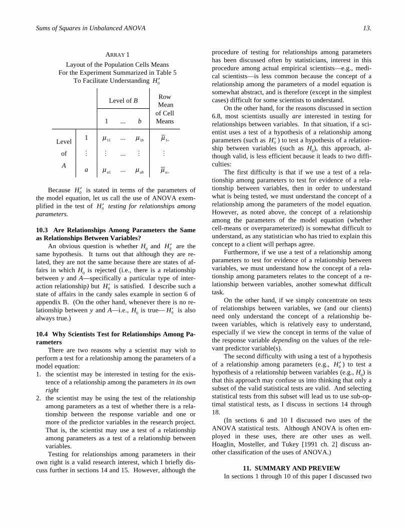
appearing in the experiment.To understand ¢H0 it is helpful to arrange the popu-

lation means for all the cells in the group treatment tablein a two-dimensional array, with the values of predictorvariable A indexing the rows and the values of predictorvariable B indexing the columns, as in array 1.

(The a and b in the array are the number of differentvalues appearing in the experiment of predictor variablesA and B respectively.)

The rightmost column in the array contains the meanof the cell means for each row. That is

m mi ijjb∑ = Â / .

Thus in terms of array 1, the hypothesis ¢H0 statesthat if we compute the mean of the population cell meansfor each row in the array, then these row means will all beequal to one another.


procedure of testing for relationships among parametershas been discussed often by statisticians, interest in thisprocedure among actual empirical scientists—e.g., medi-cal scientists—is less common because the concept of arelationship among the parameters of a model equation issomewhat abstract, and is therefore (except in the simplestcases) difficult for some scientists to understand.

On the other hand, for the reasons discussed in section6.8, most scientists usually are interested in testing forrelationships between variables. In that situation, if a sci-entist uses a test of a hypothesis of a relationship amongparameters (such as ¢H0 ) to test a hypothesis of a relation-ship between variables (such as H0), this approach, al-though valid, is less efficient because it leads to two diffi-culties:

The first difficulty is that if we use a test of a rela-tionship among parameters to test for evidence of a rela-tionship between variables, then in order to understandwhat is being tested, we must understand the concept of arelationship among the parameters of the model equation.However, as noted above, the concept of a relationshipamong the parameters of the model equation (whethercell-means or overparameterized) is somewhat difficult tounderstand, as any statistician who has tried to explain thisconcept to a client will perhaps agree.

Furthermore, if we use a test of a relationship amongparameters to test for evidence of a relationship betweenvariables, we must understand how the concept of a rela-tionship among parameters relates to the concept of a re-lationship between variables, another somewhat difficulttask.

On the other hand, if we simply concentrate on testsof relationships between variables, we (and our clients)need only understand the concept of a relationship be-tween variables, which is relatively easy to understand,especially if we view the concept in terms of the value ofthe response variable depending on the values of the rele-vant predictor variable(s).

The second difficulty with using a test of a hypothesisof a relationship among parameters (e.g., ¢H0 ) to test ahypothesis of a relationship between variables (e.g., H0) isthat this approach may confuse us into thinking that only asubset of the valid statistical tests are valid. And selectingstatistical tests from this subset will lead us to use sub-op-timal statistical tests, as I discuss in sections 14 through18.

(In sections 6 and 10 I discussed two uses of theANOVA statistical tests. Although ANOVA is often em-ployed in these uses, there are other uses as well.Hoaglin, Mosteller, and Tukey [1991 ch. 2] discuss an-other classification of the uses of ANOVA.)

11. SUMMARY AND PREVIEWIn sections 1 through 10 of this paper I discussed two

ARRAY 1

Layout of the Population Cells MeansFor the Experiment Summarized in Table 5

To Facilitate Understanding ¢H0

Level of BRow

Mean

1 ... bof CellMeans

Level1 m11 ... m1b m1∑

of M M ... M M

Aa m a1 ... m ab m a∑

Because ¢H0 is stated in terms of the parameters ofthe model equation, let us call the use of ANOVA exem-plified in the test of ¢H0 testing for relationships amongparameters.

10.3 Are Relationships Among Parameters the Sameas Relationships Between Variables?

An obvious question is whether H0 and ¢H0 are thesame hypothesis. It turns out that although they are re-lated, they are not the same because there are states of af-fairs in which H0 is rejected (i.e., there is a relationshipbetween y and A—specifically a particular type of inter-action relationship) but ¢H0 is satisfied. I describe such astate of affairs in the candy sales example in section 6 ofappendix B. (On the other hand, whenever there is no re-lationship between y and A—i.e., H0 is true— ¢H0 is alsoalways true.)

10.4 Why Scientists Test for Relationships Among Pa-rameters

There are two reasons why a scientist may wish toperform a test for a relationship among the parameters of amodel equation:1. the scientist may be interested in testing for the exis-

tence of a relationship among the parameters in its ownright

2. the scientist may be using the test of the relationshipamong parameters as a test of whether there is a rela-tionship between the response variable and one ormore of the predictor variables in the research project.That is, the scientist may use a test of a relationshipamong parameters as a test of a relationship betweenvariables.Testing for relationships among parameters in their

own right is a valid research interest, which I briefly dis-cuss further in sections 14 and 15. However, although the


uses of the ANOVA statistical tests, namely:• to test for relationships between variables (section 6) and• to test for relationships among the parameters of the

model equation (section 10).I noted that scientists are often interested in testing forrelationships between variables. In sections 12 through 18I will discuss two methods of computing ANOVA sums ofsquares and will evaluate the two methods of computingsums of squares for fulfilling the two uses of the ANOVAstatistical tests.

12. RESIDUAL SUMS OF SQUARESIn sections 9.3 - 9.6 of this paper I noted that for any

overparameterized model equation, and for the results ofany research project that is consistent with the modelequation and that has no empty cells in the group treat-ment table, we can (using the method of least squares andpossibly using the sigma restrictions) “fit” the equation tothe results of the research project and thereby obtain esti-mates of the values of the parameters in the equation.

For example, suppose we have performed the 2 ¥ 3experiment summarized in table 5. In section 9.3 I notedthat this experiment has the following overparameterizedmodel equation:

yijk i j ij ijk= + + + +m a b f e . (3)

In section 9.4 I noted that we can use the method of leastsquares to fit (3) to the results of the experiment andthereby obtain estimates of the values of the m , a ’s,b ’s, and f ’s in the equation for the population of entitieswe are studying.

I also noted that once we have obtained estimates ofthe values of the parameters, we can then substitute theappropriate estimates into the model equation to predictthe value of the response variable for each entity in eachcell in the group treatment table in the research project.(Of course, for any given cell in the group treatment table,the predicted value for all the entities in the cell is thesame.)

Using the foregoing ideas, let us consider a definitionof the concept of a residual sum of squares:

Definition: For any research project in which the re-sponse variable has numeric values, the residual sumof squares of a model equation in the research projectis the sum across all the values of the response vari-able in the research project of the squared deviationof the value predicted by the model equation for anentity from the actual measured value of the responsevariable in the entity. That is, for any model equationin a research project, the residual sum of squares is

SSr measured predicted= -Â( ) .2

It is, of course, the residual sum of squares that the

least-squares procedure minimizes in order to determinethe estimates of the values of the parameters. I use theconcept of the residual sum of squares of a model equa-tion shortly.

13. TWO METHODS OF COMPUTINGANOVA SUMS OF SQUARES

A critical step in computing the p-values in anANOVA is to compute different “sums of squares” fromthe results of the experiment. (Please distinguish ANOVAsums of squares from the closely related residual sums ofsquares discussed in the preceding section.) Variousmethods of computing ANOVA sums of squares are avail-able, two of which I discuss in this section.

We can characterize both methods of computingANOVA sums of squares in terms of the difference be-tween the residual sums of squares of two model equations(Yates 1934:63, Scheffé 1959, Searle 1971). I shall callthese equations the two generating equations for anANOVA sum of squares.

13.1 The HTO Method of Computing Sums of SquaresOne method of computing ANOVA sums of squares

is to have Higher-level Terms Omitted from the two gen-erating model equations (HTO). For example, if we haveperformed the experiment summarized in table 5, then un-der the HTO method we can compute the ANOVA sum ofsquares for the A simple relationship (main effect) by firstfitting (separately) the following two new model equationsto the data:

yijk j ijk= + +m b e (7)

yijk i j ijk= + + +m a b e (8)

where in each equation (if the associated term is present):

a iiÂ = 0

b jjÂ = 0.

Then under the HTO method, the sum of squares forthe A simple relationship is the residual sum of squares for(7) minus the residual sum of squares for (8). [This dif-ference will always be non-negative because (8) has anadditional term, and thus will always provide at least asclose a fit to the data as (7).] Thus (7) and (8) are thegenerating model equations for the HTO sum of squaresfor the A simple relationship for the experiment.

By examining (7) and (8) we can see that under theHTO method of computing sums of squares we are testingthe effect on y of a change in the value of variable A bystudying the reduction in the residual sum of squares if weinclude a term for variable A in the model equation, usinga model equation with no interaction term. It is custom-


ary to say that the interaction term is a higher-level termthan the A term because the interaction term refers to twoof the predictor variables (i.e., A and B) while the A termrefers to only one. I use the name HTO to reflect the factthat (although terms at the same level are included)Higher-level Terms are Omitted from the two generatingmodel equations.

Generating equations (7) and (8) are called unsatu-rated model equations because not all the possible termsin the standard overparameterized model equation for theexperiment [i.e., equation (3)] are included in the equa-tions. We can always use the least-squares procedure toobtain estimates of the values of the parameters in an un-saturated overparameterized model equation. If we wish,we can use sigma restrictions to facilitate the solution.

The procedure of computing an HTO sum of squaresby computing the difference in the residual sums ofsquares of two generating model equations illustrates whatis being computed when we compute the sum of squares.There are, of course, computationally or algebraicallymore efficient (but conceptually less transparent) proce-dures for performing the same computation as discussedbriefly in the second part of appendix C. For detailedcoverage of the methods, see the landmark discussions byHocking (1985) and Searle (1987).

13.2 The HTI Method of Computing Sums of SquaresA second method of computing ANOVA sums of

squares is to have Higher-level Terms Included in the twogenerating model equations (HTI). For example, if wehave performed the experiment summarized in table 5,then under the HTI method we can compute the ANOVAsum of squares for the A simple relationship by first fitting(separately) the following two model equations to thedata:

yijk j ij ijk= + + +m b f e (9)

yijk i j ij ijk= + + + +m a b f e (10)

where we use the sigma restrictions from (4).Then under the HTI method, the sum of squares for

the A simple relationship is the residual sum of squares for(9) minus the residual sum of squares for (10).

By examining (9) and (10) we can see that under theHTI method of computing sums of squares we are testingthe effect on y of a change in the value of variable A bystudying the reduction in the residual sum of squares if weinclude a term for variable A in the model equation, butthis time we are using model equations with an interactionterm. I use the name HTI to reflect the fact that (in addi-tion to including terms at the same level) Higher-levelTerms are Included in the two generating model equa-tions.

[On a technical matter, in unsaturated generating

model equations, in addition to allowing us to obtainunique estimates of the value of the parameters, some ofthe sigma restrictions play a second role: they prevent theinteraction terms in the model equation from wrongly ac-counting for variation in the values of the response vari-able that should be accounted for by lower-level terms or,as in (9), that should not be accounted for at all. This ap-proach, which is entailed by the principle that each inter-action term in a model equation should be independent ofthe effects of all of the other terms, solves a problemidentified by Searle (1971, 1987:339-340) and Nelder(1977:50) concerning certain ANOVA sums of squaresthat would undesirably turn out to be zero.]

13.3 General CommentsI have illustrated the HTO and HTI methods of com-

puting ANOVA sums of squares in terms of an experimentwith two predictor variables. The distinction between thetwo methods can be generalized to include experimentswith any number of predictor variables by noting that wecan view each method in terms of fitting two generatingmodel equations to the data: one equation containing theterm for the effect being tested, and the other equationlacking the term for the effect being tested. And the de-sired sum of squares is the difference between the residualsums of squares of the two generating equations. In com-puting the HTO sums of squares, Higher-level Terms areOmitted from the two generating equations although (withone obvious exception) all the terms at the same level as,and at lower levels (if any) than, the effect being testedare included. On the other hand, in computing the HTIsums of squares, all the Higher-level Terms are Includedin the two generating equations along with all the terms atthe same and lower levels (with the same one exception).

The HTO and HTI methods of computing ANOVAsums of squares generally yield numerically different val-ues from each other in an unbalanced experiment. How-ever, they always yield identical values in a balanced ex-periment. Furthermore, in a balanced experiment the twomethods yield sums of squares that are identical to thesums of squares obtained through the standard ANOVAtechniques for balanced experiments.

In a fully crossed unbalanced experiment with two ormore predictor variables (and with no empty cells), it canbe shown that the HTO and HTI sums of squares for thehighest-level interaction are always identical. Similarly,in an unbalanced experiment with only a single predictorvariable, it can be shown that the HTO and HTI sums ofsquares for the simple relationship are always identical.

Table 7 shows the names that twelve articles andeight statistical computer programs use for the HTO andHTI methods of computing ANOVA sums of squares inexperiments with two predictor variables.


TABLE 7

Names Used by Twelve Articles and Eight Computer Programsfor Two Methods of Computing Sums of Squares

in Two-Way Unbalanced ANOVA _________________________________________________________________________________

Reference HTO HTI _________________________________________________________________________________

ARTICLES

Yates (1934) fitting constants weighted squares of means

Overall and Spiegel (1969) method 2 method 1

Burdick et al (1974) method 2 method 1

Kutner (1974) hypotheses F and G hypotheses A and B

Hocking and Speed (1975) hypotheses HA** and HB** hypotheses HA and HB

Speed and Hocking (1976) hypotheses 5 and 6 hypotheses 1 and 2

Herr and Gaebelein (1978) EAD (method 3) STP (method 1)

Speed, Hocking, and Hackney (1978) hypotheses 3 and 7 hypotheses 1 and 5

Burdick (1979) hypothesis 3 hypothesis 1

Elliott and Woodward (1986) hypotheses 3 and 6 hypotheses 1 and 2

Milligan et al (1987) hypothesis H3 and H7 hypothesis H1 and H5

Singh and Singh (1989) hypotheses H5 and H6 hypotheses H1 and H2

COMPUTER PROGRAMS

SAS GLM (SAS Institute 1990:109) Type II Type III

SPSS ANOVA (SPSS 1990:64) method = experimental method = unique

SPSS MANOVA (SPSS 1990:377) - unique method

BMDP 4V (Dixon 1990a:1155) weights = sizes weights = equal

BMDP 2V (Dixon 1990b:489) - default method

SYSTAT MGLH (Wilkinson 1990:140) - default method

MINITAB GLM (Minitab 1989:8-27) - default method

Data Desk Linear Models (Velleman n.d.:39) - Partial (Type 3) _________________________________________________________________________________

Table 7 covers only two-way experiments. For three-way and higher experiments, the SPSS ANOVA EX-PERIMENTAL sums of squares are identical to HTOsums of squares. However, for three-way and higher ex-periments, although some SAS type II sums of squares andsome BMDP4V WEIGHTS = SIZES sums of squares areidentical to HTO sums of squares, others are not. (Nor arethe SAS type II sums of squares and the correspondingBMDP4V WEIGHTS = SIZES sums of squares alwaysidentical to each other.) Davidson and Toporek (1979:21)compare sums of squares from the three statistical pack-ages for two- and three-way experiments. In their com-parison the SPSS-D (for “default”) sums of squares areidentical to what are now called SPSS ANOVA EX-PERIMENTAL sums of squares and URWAS is the old

name for the computer program that is now calledBMDP4V.

If you need to compute an HTO (or certain othertypes of) sum of squares, but if the available statisticalpackage cannot do the computation directly, then (withmost packages) you can do the computation indirectly byusing the following steps for each sum of squares youwish to compute:• Specify to the linear regression program in the package

the first of the two generating model equations for thesum of squares and then use the regression program tocompute the residual sum of squares for that modelequation. (Use full-rank dummy-variable specifica-tion—which has the same effect as imposing sigma re-strictions—in this and the next step in order to bypass


the problem discussed in the last paragraph of section13.2.)

• Specify to the regression program the second of the twogenerating equations and then use the program to com-pute the residual sum of squares for that equation.

• Subtract the smaller residual sum of squares from thelarger to yield the associated ANOVA sum of squares.

Alternatively, you can obtain the same result usingthe matrix arithmetic procedure given in the second partof appendix C.

14. THE HTO METHOD IS GENERALLYINAPPROPRIATE WHEN TESTING FOR

RELATIONSHIPS AMONG PARAMETERSI have now discussed:

• using ANOVA to test for relationships between variablesand using ANOVA to test for relationships among theparameters of the model equation (sections 6 and 10 re-spectively)

• the HTO and HTI methods of computing ANOVA sumsof squares (section 13).

In this and the next three sections I address the ques-tions of which of the HTO and HTI methods is better fortesting for relationships between variables, and which isbetter for testing for relationships among parameters. Ibegin by considering the HTO method and testing for re-lationships among parameters.

Several authors have correctly noted that the HTOmethod of computing sums of squares is generally not ap-propriate if we wish to test for relationships among pa-rameters (Carlson and Timm 1974, Kutner 1974, Speed,Hocking, and Hackney 1978, Hocking, Speed, and Cole-man 1980, Searle 1987). These authors have shown that,in general, under the testing for relationships among pa-rameters approach, the HTO method does not test mean-ingful, useful, or interesting hypotheses.

For example, consider the two-way ANOVA for theexperiment summarized in table 5. Searle (1987:115)notes that the HTO sum of squares for the A simple rela-tionship (main effect) in this experiment enables us to testwhether the following relationship exists among the pa-rameters of (2), the associated cell-means model equation:

nn n

niij ijj

ij tj

jtjtj

m mÂ ÂÂ= "∑

(11)

where:nij = number of entities in the ij cell in the group treat-

ment table and

n nj iji∑ = Â .

Searle also notes (1987:333) that the same HTO sumof squares for the A simple relationship enables us to test

whether the following relationship exists among the pa-rameters of (3), the associated overparameterized modelequation:

nn n

niij i ijj

ij tj

jt tjtj

( ) ( ) .a f a f+ = + "Â ÂÂ∑

(12)

The important question is whether either of these testsof relationships among the parameters in an unbalancedexperiment is of any use. And, as the authors cited abovehave noted, scientists are virtually never specifically inter-ested in testing whether the (equivalent but somewhat ar-cane) relationships shown in (11) and (12) exist among theparameters of the model equation. This example illus-trates why the HTO method of computing sums of squaresis generally inappropriate if our goal is to test for relation-ships among parameters.

15. BUT THE HTI METHOD IS APPROPRIATEWHEN TESTING FOR RELATIONSHIPS

AMONG PARAMETERSOn the other hand, Searle (1987:335) notes that the

HTI test for the A simple relationship (main effect) testswhether the following relationship (discussed earlier insection 10.2) exists among parameters of the cell-meansmodel equation:

¢ "ÂH b iijj0: / .m equal (6)

Similarly, Searle (1987:335) notes that the same HTItest for the A simple relationship tests whether the follow-ing relationship exists among the parameters of the over-parameterized model equation:

a fi ijjb i+ "Â / .equal (13)

If the sigma restrictions are imposed, the relationshipin (13) reduces to:

a i i= "0 . (14)

The relationships shown in (6), (13), and (14) arerelatively easy to understand and are relationships amongparameters that scientists are sometimes interested intesting.

Because statisticians have endorsed the HTI methodof computing ANOVA sums of squares (because the as-sociated statistical tests test hypotheses of interest for re-lationships among parameters), and because many scien-tists are not familiar with the facts discussed below, manyscientists choose the HTI method of computing sums ofsquares in unbalanced ANOVA even when they are notinterested in testing for relationships among parameters,but are instead actually interested in testing for relation-ships between variables. Unfortunately, as I shall discussbelow, this choice is sub-optimal.


16. BOTH THE HTO AND HTI METHODSARE APPROPRIATE WHEN TESTING

FOR RELATIONSHIPS BETWEENTHE RESPONSE VARIABLE AND

THE PREDICTOR VARIABLESIn the preceding two sections I reviewed the well-

known conclusions that the HTO sums of squares are gen-erally not appropriate if our goal is to test for relationshipsamong parameters while the HTI sums of squares are gen-erally appropriate for that goal. That review was includedto help readers contrast its conclusions with the main ar-gument of this paper. Let me now return to the main ar-gument and evaluate the HTO and HTI methods of com-puting sums of squares if our goal is to test for relation-ships between the response variable and the predictorvariables in the population of entities under study in anexperiment.

I begin with a definition of a valid statistical test for arelationship between variables:

Definition: In situations in which the associated un-derlying assumptions are satisfied, an F-ratio-basedstatistical test for a relationship between variables is avalid test if:• in the absence of the indicated relationship the F-

ratio yielded by the test can be shown to have acentral F-distribution with known degrees of free-dom and

• in the presence of the indicated relationship the ex-pected value of the numerator of the F-ratio can beshown to be greater than the expected value of thedenominator.

The definition implies that if an ANOVA statisticaltest for a relationship between variables is valid (and if theunderlying assumptions of ANOVA are adequately satis-fied), we can then be confident that the p-values that areyielded by the test are correct estimates of the probabili-ties that they purport to estimate. Obviously, it is impor-tant that ANOVA statistical tests for relationships betweenvariables be valid.

Let us now consider a theorem that shows that theHTO sums of squares provide valid statistical tests for re-lationships between variables in certain general situations:

Theorem 1 (proved in appendix A): Consider an n-way fully crossed research project (where n > 1) withno empty cells in the group treatment table. Supposethat the underlying assumptions of ANOVA are satis-fied. Select any q of the predictor variables where 1£ q < n. Suppose that there are no (q + 1)-way orhigher-way population interactions involving all ofthe q selected predictor variables (it being only neces-sary to consider variables measured in the researchproject). Then the HTO statistical test that is associ-ated with the q predictor variables is a valid test if we

wish to test for evidence of a q-way population rela-tionship between the q selected predictor variableswith respect to their joint relationship to the responsevariable. (That is, if q > 1, the test is a valid test forthe presence of the q-way interaction, and if q = 1, thetest is a valid test for the presence of the simple rela-tionship.) Similarly, the n-way HTO test is a validtest if we wish to test for evidence of an n-way popu-lation interaction between all of the predictor vari-ables with respect to their joint relationship to the re-sponse variable.

Put simply, theorem 1 implies that the HTO sums ofsquares are (with one qualification, and if the underlyingassumptions are adequately satisfied) valid for use in sta-tistical tests if our purpose is to test the results of a re-search project for evidence of a population relationshipbetween the response variable and the predictor variables.

Theorem 1 can also be proven for statistical tests thatare based on the HTI sums of squares.

Thus both the HTO and HTI sums of squares are ap-propriate for testing for population relationships betweenthe response variable and the predictor variables in an ex-periment, at least in the absence of associated higher-levelinteractions.

I discuss why higher-level interactions usually do notcreate problems when scientists are testing for relation-ships between variables in appendix B.

17. THE HTO METHOD IS GENERALLY MOREPOWERFUL THAN THE HTI METHOD

WHEN TESTING FORRELATIONSHIPS BETWEEN VARIABLES

Definition: If• we apply an ANOVA statistical test of a relation-

ship between variables to the results of a researchproject and

• the underlying assumptions of ANOVA are ade-quately satisfied and

• (most importantly) the p-value that is yielded by thetest is less than or equal to the critical p-value thatwe have chosen for the test (i.e., usually .05 or .01),

then we say that the statistical test provides reason-able evidence that the relationship exists.

Using the concept of providing reasonable evidencethat a relationship exists, let us now define the power of astatistical test.

Definition: For a given form of a relationship be-tween variables, the power of a statistical test of therelationship is the fraction of the times that the test isperformed (each time with a fresh random samplefrom the population of interest) that the test will pro-vide reasonable evidence that the relationship exists,given that the relationship has the specified form.


Within the limits of time and cost constraints,scientists generally prefer to use statistical tests that (whenoperating in the vicinity of the expected form of the rela-tionship) have the highest possible power because suchtests are more likely to discover the sought-after relation-ship, if it exists. Thus having noted that both the HTOand HTI sums of squares are appropriate for testing forrelationships between the response variable and the pre-dictor variables, an important question is: Of the HTOand HTI methods of computing sums of squares, whichmethod yields more powerful statistical tests for detectingrelationships between variables?

Theorem 2 (proved in appendix C): Consider an n-way fully crossed research project (where n > 1) withno empty cells in the group treatment table. Supposethat the underlying assumptions of ANOVA are satis-fied. Select any q of the predictor variables where 1£ q < n. Suppose that there are no (q + 1)-way orhigher-way population interactions among the predic-tor variables in the research project with respect totheir joint relationship to the response variable. Thenif a q-way population interaction (or, if q = 1, a sim-ple relationship) exists between the selected predictorvariables with respect to their joint (its) relationshipto the response variable, the statistical test (usingwithin-cell error) for the q-way interaction (or, if q =1, for the simple relationship) based on the HTO sumof squares is at least as powerful for detecting the in-teraction (simple relationship) as the statistical test(also using within-cell error) based on the HTI sum ofsquares.

Theorem 2 implies that an HTO statistical test is, un-der certain general conditions, at least as powerful for de-tecting relationships between variables as the associatedHTI statistical test. However, because the two tests haveexactly the same power only when special conditions ob-tain, usually in unbalanced experiments the HTO test ismore powerful than the HTI test. Of course, the size ofthe difference in power between the two tests depends onthe pattern of imbalance in the experiment. (Littell andLynch [1983] examine the simplest case.) Furthermore,often the difference in power will be small. However,given the possible high social cost of a failure to discovera useful existing relationship between variables, the dif-ference in power is large enough to be a considerationwhen deciding which method of computing sums ofsquares to use when testing for relationships between vari-ables.

You can easily empirically see the validity of theorem2 by analyzing several sets of unbalanced experimentaldata with an unbalanced ANOVA computer program thatcan compute both types of sums of squares. (Of course,for each experiment there must be no empty cells in the

group treatment table, the data must contain evidence of arelationship, and the experiment must have two or morepredictor variables.) Except for the highest-level interac-tion (for which the HTO and HTI sums of squares areidentical), whenever an effect is significant, the HTO sumof squares for the statistical test will usually (but not al-ways) be larger than the corresponding HTI sum ofsquares, and thus the p-value for the HTO sum of squareswill usually be smaller than the p-value for the HTI sumof squares, which indirectly implies that statistical testsbased on the HTO method of computing sums of squaresare generally more powerful.

Theorem 2 implies that statistical tests based on theHTO method of computing sums of squares are preferredto statistical tests based on the HTI method in ANOVA ofunbalanced experiments with no empty cells when thereare no higher-level interactions if (as is often the case) ourgoal is to test for relationships between the response vari-able and the predictor variables. That is the main point ofthis paper.

I discuss an extension to the HTO approach for three-way and higher experiments in appendix D and I discussother approaches to ANOVA statistical tests in appendixE.

18. SUMMARYEntities, properties of entities, and relationships be-

tween properties of entities are fundamental concepts ofhuman thought. In science, properties are roughly syn-onymous with variables. Relationships between variablesare of central concern to scientists.

Two uses of the ANOVA statistical tests are:• to test for population relationships between the response

variable and the predictor variables in an experiment• to test for population relationships among the parameters

of the model equation in an experiment.Two popular approaches for computing ANOVA

sums of squares are the HTO approach or the HTI ap-proach.

If we wish to test for relationships between the re-sponse variable and the predictor variables in an experi-ment, both the HTO and HTI approaches are appropriate(valid).

Main point: If we wish to use ANOVA to test forevidence of relationships between variables in an experi-ment with no empty cells, statistical tests based on theHTO approach are preferred to statistical tests based onthe HTI approach because the former tests are generallyslightly more powerful.

APPENDIX A: PROOF OF THEOREM 1The following proof is a generalization of the first

part of a theorem proved in the two-way case by Burdick


and Herr (1980:239):As exemplified by Searle (1987), for any given HTO

ANOVA statistical test, the hypothesis being tested can beshown in terms of one or more expressions that containonly terms in parameters of the overparameterized modelequation. Furthermore, for a given HTO test, these ex-pressions contain only terms in the parameters associatedwith (a) the effect being tested and (b) the associatedhigher-level interactions. For example, see (12).

(*) For any q-way effect in an overparameterizedmodel equation (i.e., an effect for a particular interactionor an effect for a particular simple relationship), if:• there are no associated higher-level interactions in the

population between the predictor variable(s) associatedwith the effect and other predictor variables in the re-search project with respect to their joint relationship tothe response variable and

• there is no associated q-way relationship in the popula-tion between the predictor variable(s) associated withthe effect with respect to their (its) joint relationship tothe response variable

then the parameters in the overparameterized model equa-tion that are associated with the effect will be all identical.(This can be derived from the definition of interactive andsimple relationships between variables and from thedefinition of an overparameterized model equation.)

If the parameters associated with a higher-level inter-action in an expression of a hypothesis being tested are allidentical, we can remove any terms that are associatedwith that interaction from the expression of the hypothesisin order to obtain a more succinct statement of the hy-pothesis. (This can be seen by examining the expressionsof the hypothesis being tested such as (12) and noting thatif the f ij ’s are all replaced by a constant k, then the corre-sponding statement of the hypothesis with the k’s omittedcan be derived from the statement with the k’s includedthrough some minor algebra.)

If we remove all the higher-level interaction termsfrom the expressions of a hypothesis, examination of theresulting expressions reveals that the test is a test (using aweighting to reflect the relative accuracy of the estimatedvalues of the parameters) of whether all the parameters as-sociated with the effect in question are identical. (Thiscan be seen in (12) by noting that if the f ' s are all re-moved, and if the a ’s in the i expressions are all setidentical to some value k, then the expressions in (12) allbecome tautologically true.)

But from (*) if there is no associated higher-level in-teraction and no q-way relationship, the parameters asso-ciated with the effect will all be identical.

Thus if there is no associated population higher-levelinteraction and no population q-way relationship, the ex-pression of the hypothesis associated with the HTO sum ofsquares will be satisfied, and thus (if the underlying as-

sumptions of ANOVA are satisfied) the numerator meansquare and the denominator mean square in the F-ratiowill have the same expected value. Thus if there is no as-sociated population higher-level interaction and no popu-lation q-way relationship, (and if the underlying assump-tions of ANOVA are satisfied), the HTO F-ratio will havea central F-distribution. And thus the HTO statistical testsatisfies the first part of the definition of a valid ANOVAstatistical test.

On the other hand, if there is a visible (within thecontext of the experiment) population relationship be-tween the predictor variable(s) associated with the effectof interest with respect to their joint (its) relationship tothe response variable (but there is no associated higher-level interaction), then the parameters associated with theeffect will not be all identical and thus, because the termassociated with those non-identical parameters is omitted,the model equation with the omitted term [e.g., (7)] willhave an inflated residual sum of squares. Thus the effectmean square based on the difference of the residual sumsof squares of the two model equations [e.g., (7) and (8)]will have an expected value that is greater than the errormean square. Thus the expected value of the numerator ofthe HTO F-ratio will be greater than the expected value ofthe denominator. And thus the HTO statistical test satis-fies the second part of the definition of a valid ANOVAstatistical test.

And thus the theorem is proved.

APPENDIX B: HIGHER-LEVEL INTERACTIONSIn this appendix I discuss why the qualification about

higher-level interactions given at the end of section 16usually does not create problems when scientists are test-ing for relationships between variables.

B.1 A Reasonable Approach to ANOVAScientists who are testing for relationships between

variables usually use ANOVA to help them answer thefollowing two questions:• As x1 changes in an entity, can we also expect y to

change in the entity? That is, is there a relationshipbetween x1 and y?

• Given that there is a relationship between x1 and y inentities, does the profile of the relationship depend onthe level of x2, x3, ... in the entities? That is, is the rela-tionship an interactive relationship?

A reasonable approach to answering these questions is(after performing an appropriate experiment) to examinethe components (rows) in the ANOVA table beginningwith the highest-level interaction and working down to thesimple relationships (main effects). As we work down, ifwe find a significant component, we can tentatively con-clude that there is a relationship between (a) the responsevariable and (b) the set of one or more predictor variables


that are associated with the component. (Of course, if ppredictor variables are associated with a significant com-ponent, where p > 1, we can tentatively conclude thatthere is a p-way interaction between the p predictor vari-ables with respect to their joint relationship to the re-sponse variable.)

Let us use the term associated lower-level compo-nents to refer to components in an ANOVA table that areassociated only with predictor variables that are all in-volved in a particular higher-level interaction. For exam-ple, consider a four-way ANOVA in which the predictorvariables are A, B, C, and D, and consider the A ¥ B ¥ Cinteraction. Then the associated lower-level componentsfor this interaction are all the components in the ANOVAtable that contain one or two of variables A, B, and C.There are six such components, namely A, B, and C, and A¥ B, A ¥ C, and B ¥ C.

After finding a significant component in an ANOVAtable, we can continue (in the order mentioned above)checking components in the table. However, as suggestedby Appelbaum and Cramer (1974:340), Aitkin (1978:200),and Cox (1984:16) if we are seeking evidence of relation-ships between variables, once we have found a significantinteraction component we are usually not interested in anyof the associated lower-level components. We are usuallynot interested in these components because the higher-level interaction will have already told us that there is arelationship between the response variable and the asso-ciated predictor variables, and the relationship is interac-tive at the indicated level. And if we are seeking evidenceof relationships between variables, checking the associ-ated lower-level components will usually give us no fur-ther useful information (beyond giving us more evidencethat the relationship exists).

Some writers disagree with the preceding sentence.Sections B.2 - B.5 address arguments that have been madein favor of checking associated lower-level componentsfor statistical significance in the presence of a significanthigher-level interaction.

B.2 Lower-Level Relationships Cannot Be Present inthe Presence of a Higher-Level Associated Interaction

One argument in favor of checking the associatedlower-level components is that such checking enables usto see whether simple relationships or lower-level interac-tions exist between the response variable and the associ-ated predictor variables. However, if there is an interac-tion between two or more predictor variables with respectto their joint relationship to the response variable, then(for reasons given below) a simple relationship betweenthe response variable and any of the predictor variablesinvolved in the interaction cannot exist. Similarly, if thereis an interaction between p predictor variables with re-spect to their joint relationship to the response variable

where p > 2, then a lower-level interaction between two ormore of the predictor variables involved in the interactionalso cannot exist. Thus if there is a significant interaction,checking the associated lower-level components of theinteraction does not allow us to see whether simple rela-tionships or lower-level interactions exist between the re-sponse variable and the associated predictor variables be-cause (for reasons given below) such simple relationshipsand interactions cannot exist.

The conclusion of the preceding paragraph is derivedfrom the definition of a simple relationship between vari-ables and from the definition of an interaction, which areboth given in section 6.10. To help understand the con-clusion, let us revisit the definitions. A critical feature ofthe definitions is that each definition contains a clause thatlimits each predictor variable to being involved in onlyone type of relationship (or no relationship) with the re-sponse variable at a time. That is, a particular predictorvariable can only be involved in a simple relationship orin a particular single interaction at a time, and another re-lationship between that predictor variable and the responsevariable cannot exist.

The fact that a given predictor variable can only beara single type of relationship to the response variable at atime is, of course, not an empirical fact, but instead sim-ply results from a definition. Thus we could easily choosesome other definition for a simple relationship or an inter-action. In particular, we could choose a definition thatallows simple relationships and interactions to exist evenin the presence of associated higher-level interactions.

However, the requirement of the definitions that apredictor variable can only bear one type of relationship tothe response variable at a time is helpful in formulating aneasily-grasped concept of a relationship between variablesbecause the requirement simplifies the concept of a rela-tionship without limiting its generality.

In particular, it is important to recognize that thedefinitions given in section 6.10 of simple and interactiverelationships between variables do not prevent us fromhaving terms for both an interaction effect and an associ-ated lower-level effect in a model equation at the sametime, if we wish. But even when we include terms ofvarious levels in a model equation, it is still perhaps sim-plest to view the relationship in terms of the highest-levelinteraction—as a single high-level interaction between allof the associated predictor variables with respect to theirjoint relationship to the response variable, rather than as acombination of two or more different relationships. Fromthis point of view, once we decide that there is an interac-tion, there is no need to examine associated lower-levelcomponents to see if there is any evidence that the asso-ciated lower-level relationships exist because (by defini-tion) they cannot.


B.3 The Final Form of the Model Equation: PracticalConsiderations

If we are using an overparameterized model equation,another argument in favor of testing the associated lower-level components for significance in the presence of asignificant higher-level interaction is that such tests tell uswhich terms to include in the final form of the modelequation. However, knowledge of whether we need toinclude a simple-effect (or lower-level interaction) term ina model equation is often of little practical use becauseoften in performing ANOVA we are not interested inknowing which terms are required in the final form of themodel equation, and we are only interested in knowingwhich relationships, if any, exist between the responsevariable and the predictor variables.

We are usually not interested in the final form of themodel equation because the model equations used inANOVA are usually of little use beyond providing a wayof understanding what is being tested in a statistical test,and for enabling analysis of the power of statistical tests,and for providing an easily-understood way of describingthe computation of sums of squares. That is, ANOVAmodel equations are not often used in substantive areas todescribe relationships between variables or to make pre-dictions. ANOVA model equations are not often used insubstantive areas because the discrete-valued terms thatsuch equations contain are cumbersome, and the same de-scriptions and predictions can be made more easily andwith better understanding from the (appropriately col-lapsed, if necessary) table of predicted means of the val-ues of the response variable for the different cells in thegroup treatment table, or (perhaps better) from a graphbased on the (appropriately collapsed) table of means.(For unsaturated model equations, we may have to obtainestimates of the values of the parameters to enable us touse the model equation to compute the associated col-lapsed predicted means, but once these means are com-puted, the parameter estimates and the model equation areof little further use.) Of course, model equations that arenot ANOVA model equations are often used in substantiveareas, especially in the hard sciences, to describe relation-ships between variables. Such model equations usuallycontain continuous terms rather than discrete-valuedterms.

B.4 The Final Form of the Model Equation: Theoreti-cal Considerations

Another argument in favor of checking the associatedlower-level components for significance in the presence ofa significant higher-level interaction is that such checkstell us which terms to include in the final form of themodel equation, and this knowledge may be useful to sci-entific theoreticians in understanding the underlying proc-esses in the entities under study.

However, model equations derived in standardANOVA are not often viewed as reflecting (in any illumi-nating way) the underlying processes in the entities be-cause the equations are designed to be capable of handlingany set of means of the values of the response variable forthe various cells in the group treatment table—that is, theequations are completely general—and (apart from show-ing which type of relationship has been found, and if in-teraction is found, that a model equation with only simpleeffect terms will not work) such completely general modelequations usually cannot provide much insight into theunderlying processes in the entities. (On the other hand,the appropriately collapsed cell means can provide usefulinsight because they can assist the theoretician to test thefit of a specific function to the data to describe the rela-tionship between the response variable and the relevantpredictor variables.)

B.5 A Graphical ArgumentThe lack of usefulness of performing a statistical test

of a simple relationship or interaction when there is evi-dence that the predictor variable(s) associated with the ef-fect or interaction are all involved in a significant higher-level interaction can also be seen in terms of graphs. Per-forming a statistical test of a lower-level relationshipwhen the predictor variable(s) associated with the rela-tionship is (are all) involved in a significant higher-levelinteraction is equivalent to looking at a collapsed graph ofthe predicted cell means of the values of the responsevariable—collapsed over all the predictor variables exceptthe variables associated with the lower-level relationship.But we should generally never collapse over predictorvariables involved in a significant interaction because theresulting graph will be concealing information about thetrue nature of the relationship between the response vari-able and the predictor variables. And predictions of thevalue of the response variable for new individual entities(in the same population under the same conditions) madeon the basis of this graph (or on the basis of the associatedcollapsed cell means) will be less accurate than predic-tions made on the basis of the graph (or cell means) of thefull interaction.

B.6 ExceptionsDespite the points made above, there are rare situ-

ations in which it is necessary to perform a lower-levelstatistical test even though an associated predictor variableis also clearly involved in a higher-level interaction.Tukey (1977) gives an example of such a situation, whichI have enhanced slightly for realism:

Suppose we work in the marketing department of acandy manufacturer, and suppose a particular brand ofcandy we sell is available in two flavors, and suppose, forbudgetary reasons, it is necessary to discontinue selling


one of the flavors and, for obvious reasons, we have de-cided to discontinue selling the flavor that has the lessersales. To evaluate the relative sales of the two flavors,consider an observational study in which the entities are arandom sample of people in the geographic area where thecandy is sold, the response variable is the volume of salesof each flavor of the candy to each person, and the predic-tor variable is the flavor of the candy. Suppose we haveperformed this (repeated measurements) study, and sup-pose we also happen to know the sex of each person whoparticipated in the study, and suppose our application ofANOVA to the data reveals that there is an interactionbetween flavor and sex with respect to their joint relation-ship to sales. That is, the difference in sales between thetwo flavors is different for females from the difference insales between the two flavors for males.

Despite the fact that we have found an interaction, westill need to know whether one flavor sells significantlybetter overall than the other, so that we can confidentlydiscontinue selling the lesser-selling flavor. Thus despitethe interaction, we still need to perform a statistical test ofthe simple relationship between flavor and sales to de-termine if we have good evidence as to which flavor sellsbetter than the other.

[Note that in performing the statistical test of thesimple relationship between flavor and sales, we shoulduse the HTO sum of squares because the HTI sum ofsquares is effectively comparing the collapsed-over-sexmean of the two cell means for the first flavor with thecollapsed-over-sex mean of the two cell means for thesecond flavor and, of course, this comparison will fail todetect a difference if the two means of the cell means areidentical. However, if the two population sales means(across sex) of the cell means are identical, and if thereare more females than males in the population (or moremales than females), this does not imply that the two fla-vors have identical sales in the population. Instead, if thepopulation ratio of females to males differs substantiallyfrom 1:1, it is possible to build a situation (specifically, aparticular type of interaction between flavor and sex) inwhich there is a substantial difference in overall salesbetween the two flavors, but the two collapsed-over-sexmeans of the population cell means are identical. In thatsituation (and in situations approaching that situation) theHTI test can be expected to fail to detect the difference inoverall sales between the two flavors. On the other hand,if the sample is random, it is not possible to build a situ-ation in which the HTO test can be expected to fail to de-tect an existing difference in overall sales between the twoflavors (although, naturally, the power of the HTO testvaries with the form of the relationship and the pattern ofimbalance).]

The candy sales example shows a practical situationin which we will still be interested in performing a statis-

tical test for a simple relationship (main effect) eventhough the predictor variable involved in the simple rela-tionship is also involved in a significant interaction.However, it is important to note that the example is un-usual because (unlike most other research projects) in theexample we are not interested in optimizing the value ofthe response variable in individual entities, but instead weare interested in optimizing (i.e., maximizing) the sum ofthe values of the response variable across all the entities inthe population. (That is, we are interested in maximizingsales across people.) If it were not for the unusual sum-ming feature of this research project, it would generallynot make sense to perform the test for the simple relation-ship in the presence of the higher-level interaction.

That is, if we wish to maximize the sales of the candyto individuals, and if there is an interaction between flavorand sex, and if we are only able to offer one flavor to eachsex, then we should offer to sell to each individual the fla-vor that sells best to that individual’s sex, with (in view ofthe interaction) it being possible that one flavor will sellbetter to one sex, and the other flavor will sell better to theother. Or, in more general terms, if we wish to predict (orpossibly control) the values of the response variable innew entities that are similar to those used in the researchproject (as opposed to wishing to predict or control thesum of the values of the response variable across suchentities), we should view the relationship between the re-sponse variable and the predictor variables in its fullcomplexity because only from that point of view can wemake the best predictions (or possibly exercise the bestcontrol).

Elston and Bush (1964:686) and Frane and Jennrich(1977) give examples that are similar to Tukey’s in thatthey reflect situations in which the scientist is interested inoptimizing the sum of the values of the response variableacross all the entities in the research project as opposed tooptimizing the value of the response variable in individualentities.

Thus despite the preceding unusual example, it is stillreasonable to conclude from the earlier arguments thatenlightened scientists will usually not be interested in ex-amining lower-level relationships between the responsevariable and the predictor variables once they have con-cluded that an associated higher-level interaction exists.

B.7 Valid Means of RebuttalNote that the arguments in sections B.2 to B.5 are not

incontrovertible because it is logically impossible to provethat no (further) reasonable use exists for a lower-leveltest in the presence of a significant associated higher-levelinteraction. Thus to disprove the arguments given in thosesections one need only describe a frequently applicablereasonable use for an associated lower-level test in thepresence of a significant higher-level interaction.


Here the important word is “reasonable”. If we viewstatistics as a tool of scientific research, any acceptableargument about a reasonable use of lower-level tests in thepresence of an associated higher-level interaction must becouchable in terms of an example of a “reasonable” sci-entific research project. Thus examples with toy data orexamples that are designed to teach statistics, but that sci-entists in a substantive area would not consider reason-able, are themselves not reasonable. And for an argumentto be convincing, it must present a situation in which anenlightened scientist (not just a statistician) who is study-ing relationships between variables would have a clearinterest in knowing whether a lower-level test is signifi-cant in the presence of a believably significant associatedhigher-level interaction. This paper claims that suchsituations, although they do occur, are rare.

Nelder (1977) and Aitkin (1978) and their discussantsgive further thoughts on the usefulness of performing astatistical test for a simple relationship or lower-level in-teraction in the presence of a higher-level interaction in-volving the same predictor variables.

B.8 Breakdown AnalysesI have discussed reasons why if we are seeking evi-

dence of relationships between variables, we are usuallynot interested in testing associated lower-level ANOVAcomponents in the presence of a believably significanthigher-level interaction. However, the procedure of test-ing associated lower-level components should be clearlydistinguished from the procedure of performing a“breakdown analysis” of an interaction. A breakdownanalysis consists of analyzing one or more subsets of thefull data. In the simplest case each subset contains datafrom only one of the levels of one of the predictor vari-ables that are in the interaction, but includes data for all ofthe levels of all of the other predictor variables that are inthe interaction. (More generally, a breakdown analysiscan include data for a subset of the levels of a subset ofthe predictor variables that are in the interaction, and canalso include data for all of the levels of some or all of theother predictor variables that are in the interaction or thatare in the experiment.) Although breakdown analysessacrifice some power and generality, their use is somet-imes justified because they can help to simplify compli-cated relationships.

B.9 Extant But Non-Significant Higher-Level Interac-tions

I have concluded that a researcher usually need not beinterested in performing statistical tests of lower-levelcomponents once he or she has decided that the associatedpredictor variables are all involved in a higher-level inter-action if the researcher is seeking evidence of relation-ships between variables. Therefore, if we are seeking evi-

dence of relationships between variables, the fact (noted atthe end of section 16) that some lower-level tests are validonly in the absence of the associated higher-level interac-tions is generally not a problem in situations in whichthere is a significant higher-level interaction because, inthat case, we are usually not interested in performing theassociated lower-level tests.

But suppose an interaction exists in the population,but a statistical test of the interaction fails to find evidenceof it. If the effects of the interaction are just below thelevel of detectability, then the presence of the interactionterms in the HTO test of a lower-level relationship maymake it more likely that the lower-level relationship testwill be significant. However, this is desirable since theexistence of the interaction implies that there is a relation-ship between the response variable and the associatedpredictor variables, and we would like at least one of ourstatistical tests to find some evidence of it.

On the other hand, if an interaction exists in thepopulation, but our statistical test of the interaction fails tofind evidence of it, then the presence of the undetectedinteraction terms in the HTO test of a lower-level relation-ship may make it less likely that the lower-level test willbe significant. Further investigation of this possibility isneeded. However, the fact [as can be seen by comparing(11) and (12) with (6), (13), and (14)] that the HTO statis-tical test appropriately weights (using the cell counts) eachof the estimates of the values of the parameters accordingto its relative accuracy while the HTI test uses no suchweighting suggests that the HTO test will not often (ifever) be less powerful than the HTI test in this specialsituation.

B.10 SummaryIn section 16 I noted that the HTO sums of squares

are appropriate if our goal is to test for evidence of a rela-tionship between variables in the absence of associatedhigher-level interactions. In this appendix I discussedwhy the qualification about higher-level interactionsusually does not give rise to problems.

APPENDIX C: PROOF OF THEOREM 2Theorem 2 was first stated for the two-way case by

Yates (1934:66). As noted by Knoke (1987), theorem 2can be derived from the fact that the maximum likelihoodestimator has maximum power in an ANOVA context, assuggested by Wald (1942). Theorem 2 was directlyproved geometrically for the two-way case by Burdick andHerr (1980:239) and algebraically for the two-way case byHocking (1985:152).

The following geometric proof for the n-way case isdue to Donald S. Burdick:

Definition: The response vector is the vector of allthe usable values of the response variable that were


obtained in a research project, one element of thevector for each usable value of the response variablethat was obtained.

Definition: The observation space is the space inwhich the response vector lies.

Definition: The population mean vector lies in theobservation space and is identical to the responsevector except that each elemental value is replaced bythe (generally unknown) population mean value of theresponse variable for the cell in the group treatmenttable associated with that element.

The definition of the population mean vector con-strains it to lie in a subspace of the observation spacecalled the estimation space. The dimension of the esti-mation space is equal to the number of cells in the grouptreatment table (although, of course, the number of com-ponents in a vector in the estimation space remains thesame as the number of components in the response vec-tor).

For any given effect E, the associated sum of squares,whether HTO or HTI, is the squared length of the projec-tion of the response vector on a subspace of the observa-tion space. The power of a statistical test of E is an in-creasing function of the noncentrality, which is in turn anincreasing function of the length of the same projection ofthe population mean vector on the subspace.

Using the standard sequential—i.e., orthogonal—partitioning we can decompose the population mean vec-tor into the sum of its projections on two subspaces of theestimation space:• the subspace of the other effects at the Same or Lower

level as E (which I call the SL subspace)• the subspace of vectors in the estimation space that are

orthogonal to the SL subspace (which I call the test sub-space).

The test subspace contains the subspace associatedwith the HTO sum of squares for E. (This is because theHTO sum of squares is identical to the next sum ofsquares in the orthogonal partitioning mentioned in thepreceding paragraph.)

The test subspace also contains the subspace associ-ated with the HTI sum of squares for E. (This is becausethe HTI sum of squares is identical to the next sum ofsquares in an orthogonal partitioning in which the othereffects at the same and lower levels and all the effects atthe higher levels have already been fitted.)

If there are no higher-level interactions, the compo-nent of the population mean vector in the test subspacelies entirely in the subspace associated with the HTO sumof squares. (This is because the HTO subspace is capableof capturing—in the absence of higher-level interac-

tions—all of the variation in the mean vector apart fromthat captured in the SL subspace.) That in turn impliesthat the component of the population mean vector in theHTI subspace is a projection of the HTO component withthe result that the HTI component is a leg of a right trian-gle of which the HTO component is the hypotenuse.Since a leg can be no longer than a hypotenuse, the non-centrality for HTI can be no greater than the noncentralityfor HTO.

And thus the theorem is proved.__________

I now summarize two simple matrix algebra proce-dures that illustrate the ideas of theorem 2. You may findit helpful to program the procedures in a matrix algebracomputer language, after which you can try them on dif-ferent datasets.

You can obtain the matrix of the projection and theresulting sum of squares for the HTO, HTI, HTOS(appendix D), or the sequential statistical tests with thefollowing procedure, which is based on a discussion byHocking (1985:152-155):• specify y, the response vector, which we assume has n

elements• specify C, a cell-means contrast matrix of the hypothesis

to be tested; C has one row for each degree of freedomin the hypothesis and it has one column for each cell inthe group treatment table; each row of C specifies a dif-ferent contrast of the cell means; collectively thesecontrasts define a hypothesis to be tested; see below fora procedure to generate different versions of C

• specify W, the counting (incidence) matrix; W has nrows and it has one column for each cell in the grouptreatment table; an entry in a cell of W is 1 if the y-valueassociated with the row is associated with the group-treatment-table cell that is associated with the column,and zero otherwise

• compute H, a response-vector contrast matrix of the hy-pothesis to be tested, by using W to scale C:

H = C(W'W)-1W'H has one row for each degree of freedom in the hy-pothesis and n columns

• compute P, the response-vector projection matrix, bysquaring and normalizing H:

P = H'(HH')-1H (15)P has n rows and n columns

• compute p, the projection of the response vector:p = Py

p has n elements• compute SS, the desired ANOVA sum of squares, by

computing the squared length of p:SS = p'p.

Graybill (1983:69-76, 434-437) discusses the algebraof projections.


If you are using a matrix algebra computer package todo the arithmetic, specifying C is the only difficult step inusing the foregoing procedure. (Of course, the rows of Care simply variations of the contrasts that are used in thebalanced case. These variations can be obtained by mul-tiplying the balanced-case coefficients in a row by variousfunctions of the cell counts.) For the two-way case youcan derive different versions of C from (6) and (11) orfrom the formulas given by Speed, Hocking, and Hackney(1978, table 1), Herr and Gaebelein (1978, table 2), andKutner (1974).

For the general case you can use the following proce-dure to generate an H matrix directly, thereby bypassingthe need to specify C and W. Page references below areto Searle’s Linear Models for Unbalanced Data (1987)and references to IML are to the SAS IML User’s Guide(SAS Institute, 1988):• specify the full (but not necessarily saturated) over-

parameterized model equation [e.g., (8) above] and thereduced overparameterized model equation [e.g., (7)above] whose residual sums of squares you wish to dif-ference to obtain the desired sum of squares

• specify a simple full-rank design sub-matrix for eachpredictor variable in the ANOVA; a simple full-rankdesign sub-matrix has n rows and it has as many col-umns as there are degrees of freedom associated with thepredictor variable (i.e., one less than the number of val-ues that the associated predictor variable had in the re-search project); each column reflects a contrast of thevalues of the response variable for different values of thepredictor variable that is associated with the sub-matrix;you can use the SAS IML DESIGNF function to gener-ate a simple full-rank design sub-matrix from the vectorof the raw values of a predictor variable

• specify full-rank design sub-matrices for all of the inter-actions; a full-rank design sub-matrix for an interactionconsists of the horizontal direct product of all the simplefull-rank design sub-matrices for predictor variables thatare associated with the interaction; you can use the SASIML HDIR function to compute horizontal direct prod-ucts of matrices

• specify X2 as the full-rank design sub-matrix for theparticular component of the ANOVA for which youwish to compute the sum of squares (that is, X2 is one ofthe design sub-matrices you specified in the precedingtwo steps)

• specify X1 as the horizontal concatenation of all of thedesign sub-matrices whose associated terms are in thefull model equation specified above including a vectorof 1’s for the constant term m but excluding the designsub-matrix for the term being tested; you can use theSAS IML horizontal concatenation operator | | to per-form horizontal concatenation of matrices

• compute M1 as defined in Searle’s equation (76) on

pages 263 and 318:

M I X X1 1 1= - +

where X+ denotes the Moore-Penrose generalized in-verse of X

• compute A as a normalized form of M1X2, as defined bySearle’s equation (82) on page 264 and equation (90) onpages 272 and 318:

A M X M X= +1 2 1 2( )

• if d is the number of degrees of freedom in the hypothe-sis, then the d rows of an H matrix are equivalent to thed characteristic vectors (eigenvectors) of A that corre-spond to the d nonzero characteristic values(eigenvalues) as shown by Searle in subsection -iv onpage 235.

After computing an H matrix with the foregoing pro-cedure, you can then, if you wish, compute a C matrixfrom H as HW.

Note that for a given approach to computing a sum ofsquares, C and H are generally not unique. That is, anyset of linearly independent vectors that generate the sub-space of the projection represent a valid statement of thehypothesis being tested (in terms of contrasts of the re-sponse vector). Of course, all the different statements ofthe hypothesis are different but equivalent expressions ofthe same test of the hypothesis that there is a relationshipbetween the response variable and the particular predictorvariable(s) associated with the test.

In particular, (M1X2)' is another statement of the hy-pothesis being tested (in terms of contrasts of the responsevector) and thus can be used in place of H in (15) to com-pute P, thereby bypassing the need to compute A and itscharacteristic vectors.

I noted above that an ANOVA sum of squares is equalto the squared length of a projection Py. Another fre-quently used general theoretical formula for computingANOVA sums of squares is the quadratic form y'Ay whereA is as defined above. Thus

y'Ay = (Py)'Py= y'(P'P)y

thus illustrating that P is simply a partitioning (“squareroot”) of A.

APPENDIX D: AN EXTENSION TO THE HTOAPPROACH FOR THREE-WAYAND HIGHER EXPERIMENTS

D.1 The HTOS Approach to Computing ANOVASums of Squares

I have concluded that for the ANOVA statistical testof any particular type of relationship (i.e., a particularsimple relationship or interaction) between the responsevariable and the predictor variables:• in the absence of higher-level interactions, the HTO


method of computing sums of squares is preferred to theHTI method

• in the presence of higher-level interactions that involveall of the predictor variables associated with the rela-tionship being tested, we are usually not interested inperforming the lower-level statistical test.

Let us now turn to the situation in which there is ahigher-level interaction in the population among some ofthe predictor variables (with respect to their joint relation-ship to the response variable) but this interaction is not as-sociated with all of the predictor variables that are asso-ciated with the particular relationship between variablesthat we are currently interested in testing. (In fact, theinteraction may not even be associated with any of thepredictor variables associated with the relationship.) Thissituation occurs in some experiments with three or morepredictor variables. As we shall see, in this situation weare sometimes interested in performing lower-level statis-tical tests in the presence of higher-level interactions, andthus it is of interest to compare various methods of com-puting the relevant sums of squares for these tests.

For example, suppose we wish to analyze the resultsof a fully crossed three-way experiment in which the pre-dictor variables are A, B, and C. We can write the satu-rated overparameterized model equation for the relation-ship between the response variable and the predictor vari-ables as:

yijkl i j k

ij ik jk

ijk ijkl

= + + ++ + +

+ +

m a b gab ag bg

abg e

( ) ( ) ( )

( ) .

where the ( ) , ( ) , ( )ab ag bgij ik jk and terms represent thethree two-way interactions and the ( )abg ijk term repre-sents the three-way interaction.

Suppose our analysis has found no evidence that pre-dictor variable A is involved in any of the interactions, andthus we are interested in testing for the A simple relation-ship (main effect). If we use the HTO approach, we willcompute the numerator sum of squares for the A statisticaltest by, in effect, differencing the residual sums of squaresof the following two generating model equations:

yijkl j k ijkl= + + +m b g e

yijkl i j k ijkl= + + + +m a b g e .

Now suppose that we have evidence (through the B¥ C statistical test) that a B ¥ C interaction is present inthe population. Then the question arises whether, as wellas including terms for predictor variables B and C as isdone in the preceding two equations, we should also in-clude a term for the B ¥ C interaction in the two generat-ing model equations. That is, the question arises whetherwe should compute the sum of squares for the A simplerelationship by differencing the residual sums of squares

of the following two model equations:

yijkl j k jk ijkl= + + + +m b g bg e( )

yijkl i j k jk ijkl= + + + + +m a b g bg e( ) .

We represent this new approach to computing sums ofsquares with the name HTOS because Higher-level Termsare Omitted except for any Significant higher-level inter-actions that are not associated with all of the predictorvariables that are associated with the effect being tested.The HTOS approach was proposed by Heiberger andLaster (1977).

Two questions arise about the HTOS approach:• Is the HTOS approach valid for testing for relationships

between the response variable and the predictor vari-ables?

• Given that the HTOS approach is valid, which approachis more powerful—HTOS, HTO, or HTI?

Although the details are beyond the scope of this pa-per, it can be shown that the HTOS approach is valid.Furthermore, it can be shown that in the presence ofhigher-level population interactions between the predictorvariables that are not associated with all of the predictorvariable(s) associated with the test (but in the absence ofhigher-level interactions that are associated with all of thepredictor variables associated with the test), the HTOSapproach generally provides a more powerful statisticaltest than either the HTO approach or the HTI approach.(Of course, when there are no such non-associated higher-level interactions, the definitions imply that the HTOS andHTO sums of squares are identical, and thus the associatedHTOS and HTO statistical tests will have identicalpower.)

Thus when we are testing for relationships betweenthe response variable and the predictor variables in unbal-anced ANOVA with no empty cells in the group treatmenttable, the HTOS sums of squares are preferred to both theHTO and the HTI sums of squares because the HTOSsums of squares generally provide slightly more powerfulstatistical tests.

D.2 The HTOS Cutoff PointWhen we use the HTOS approach in three-way and

higher experiments we need a procedure for decidingwhether to include a particular non-associated higher-levelinteraction term in the two generating model equations fora given statistical test. A reasonable procedure is to de-fine a critical p-value for such interactions, and then to usethis critical p-value as a cutoff point: If the p-value for anon-associated higher-level interaction is greater than thecutoff point, we (or the computer) form the two generatingmodel equations for the effect being tested omitting theterm for that interaction from both the model equations.But if the p-value for the interaction is less than or equal


to the cutoff point, we form the two generating modelequations for the effect being tested including the term forthat interaction in both the equations.

In choosing the cutoff point it seems a more seriouserror to omit needed terms from the generating equations(which results in a violation of the assumption of inde-pendence of the values of the error term) than to includeunneeded terms in the equations (which has no effect onthe independence of the values of the error terms), andtherefore it seems reasonable to choose a relatively highcutoff point for this procedure such as .1 or .2. A cautiousscientist may even decide to use a cutoff point of 1, whichis the limiting case. Then terms for all the non-associatedhigher-level interactions will always be included in thetwo generating model equations at a cost of a slight de-crease in power relative to the appropriate HTOS generat-ing model equations.

D.3 How To Compute HTOS Sums of SquaresCurrently, the HTOS sums of squares are not directly

available in the ANOVA or general linear model proce-dures of any of the popular statistical computer packages.However, as noted above, the HTOS sums of squares areidentical to the HTO sums of squares (which are availablein some packages) except when there are significant non-associated higher-level interactions. If the available pack-age cannot compute HTO sums of squares, or if there is anon-associated higher-level interaction, you can computethe necessary HTOS sums of squares by using the proce-dures discussed in the last two paragraphs of section 13.3.

APPENDIX E: OTHER APPROACHES TO ANOVASTATISTICAL TESTS

In addition to the HTOS, HTO, and HTI methods ofcomputing and performing ANOVA statistical tests, vari-ous other methods have been proposed. (Some of thesemethods can be defined in terms of differencing the resid-ual sums of squares of two generating model equations.)Therefore, it is useful to ask whether another methodmight be better than any of the preceding methods if wewish to test for evidence of a population relationship be-tween the response variable and the predictor variables inan experiment.

Although detailed discussion of other methods is be-yond the scope of this paper, the following criteria arereasonable for evaluating any proposed method of com-puting and performing ANOVA statistical tests if we wishto test for evidence of a relationship:• for any proposed method, the resulting tests should be

valid in the sense given in section 16• of all the valid proposed tests of a given relationship, the

test of choice should, in general, have the greatest power• to eliminate arbitrariness, the p-values obtained from a

test should not depend on an ordering of the predictor

variables (as occurs with tests based on so-called se-quential or hierarchical sums of squares) unless there isa clear rationale for using such an ordering

• to lessen the need for a formal procedure to correct forthe multiplicity of statistical tests (because such a proce-dure will often substantially diminish the power of thetests), formally only a single test should be defined foreach component in the ANOVA table (although (a) asdiscussed in the preceding section, the definition of anytest may be contingent on the outcome of logically priortests and (b) informally we may perform as many differ-ent tests as we wish to help us to understand the data)

• to lessen the need for a formal procedure to correct formultiplicity, formal tests of pooled components shouldusually be omitted

• tests can be chosen keeping in mind that they will usu-ally only be used when it is reasonable to assume thatassociated higher-level interactions are non-existent, asdiscussed in appendix B.

These criteria rule out some other methods ofcomputing and performing ANOVA statistical tests.

The importance of maximizing the power of theANOVA statistical tests (while maintaining their validity)implies that it may be reasonable to define criteria forpooling F-ratio denominator sums of squares in someANOVA situations (as discussed by Steinhorst and Ever-son 1980, and Hocking 1985:150). However, discussionof such denominator pooling should be distinguished fromthe discussion in this paper, which is about methods ofcomputing F-ratio numerator sums of squares

REFERENCESAitkin, M. 1978. The analysis of unbalanced cross-clas-

sifications (with discussion). Journal of the RoyalStatistical Society, Ser. A 141:195-223.

Aitkin, M. 1983. Unbalanced data (letter). The AmericanStatistician 37:93-94.

Allan, F. E., and J. Wishart. 1930. A method of estimat-ing the yield of a missing plot in field experimentalwork. Journal of Agricultural Science 20:399-406.

Appelbaum, M. I., and E. M. Cramer. 1974. Some prob-lems in the nonorthogonal ANOVA. PsychologicalBulletin 81:335-343.

Bancroft, T. A. 1968. Topics in Intermediate StatisticalMethods, Volume I. Ames, Iowa: Iowa State UniversityPress.

Barnett, V. 1988. “Relationship”. In Encyclopedia ofStatistical Sciences vol. 8 ed. by S. Kotz and N. L. John-son. New York: Wiley.

Box, G. E. P., W. G. Hunter, and J. S. Hunter. 1978.Statistics for Experimenters: An Introduction to Design,Data Analysis, and Model Building New York: Wiley.

Box, G. E. P., and N. R. Draper. 1987. Empirical ModelBuilding and Response Surfaces. New York: Wiley.


Bryce, G. R., D. T. Scott, and M. K. Carter. 1980. Esti-mation and hypothesis testing in linear models - Areparameterization approach to the cell means model.Communications in Statistics—Theory and Methods9:131-150.

Burdick, D. S. 1979. Rows adjusted for columns versussimple row means in two-way ANOVA: When are thetwo hypotheses equivalent? Journal of the AmericanStatistical Association 74:457-458.

Burdick, D. S., and D. G. Herr. 1980. Counterexamplesin unbalanced two-way ANOVA. Communications inStatistics—Theory and Methods 9:231-241.

Burdick, D. S., D. G. Herr, W. M. O’Fallon, and B. V.O’Neill. 1974. Exact methods in the unbalanced, two-way analysis of variance—A geometric view. Commu-nications in Statistics 3:581-595.

Calinski, T. 1982. On some problems in analyzing non-orthogonal designs. In COMPSTAT, Fifth Symposiumon Computational Statistics. International Associationfor Statistical Computing.

Carlson, J. E., and N. H. Timm. 1974. Analysis ofnonorthogonal fixed effect designs. Psychological Bul-letin 81:563-570.

Chowdhury, A. R. 1987. Are causal relationships sensi-tive to causality tests? Applied Economics 19:459-465.

Cochran, W. G., and G. M. Cox. 1957. ExperimentalDesigns 2nd ed. New York: Wiley.

Cox, D. R. 1984. Interaction (with discussion). Interna-tional Statistical Review 52:1-31.

Cox, D. R. 1958. Planning of Experiments. New York:Wiley.

Cramer, E. M., and M. I. Appelbaum. 1980. Nonorthog-onal ANOVA—Once again. Psychological Bulletin87:51-57.

Davidson, M. L., and J. D. Toporek. 1979. ANOVA WithGeneral Cell Weights. BMDP Technical Report #59.Los Angeles, CA: BMDP Statistical Software, Inc.

Dixon, W. J. 1990a. BMDP Statistical Software Manual(vol. 2). Berkeley, CA: University of California Press.

Dixon, W. J. 1990b. BMDP Statistical Software Manual(vol. 1). Berkeley, CA: University of California Press.

Elliott, A. C., and W. A. Woodward. 1986. Analysis ofan unbalanced two-way ANOVA on the microcomputer.Communications in Statistics—Simulation and Compu-tation 15:215-225.

Elston, R. C., and N. Bush. 1964. The hypotheses thatcan be tested when there are interactions in an analysisof variance model. Biometrics 20:681-698.

Finney, D. J. 1960. An Introduction to the Theory of Ex-perimental Design. Chicago: University of ChicagoPress.

Finney, D. J. 1987. Why did he not ...? The AmericanStatistician 41:244-245.

Fisher, R. A. 1935. The Design of Experiments. Edin-

burgh: Oliver and Boyd. The 8th edition of this seminalwork appears in Fisher (1990).

Fisher, R. A. 1990. Statistical Methods, ExperimentalDesign, and Scientific Inference edited by J. H. Bennett.Oxford: Oxford University Press.

Fisher, R. A., and W. A. Mackenzie. 1923. Studies incrop variation: II. The manurial response of differentpotato varieties. Journal of Agricultural Science13:311-320.

Francis, I. 1973. A comparison of several analysis ofvariance programs. Journal of the American StatisticalAssociation 68:860-865.

Frane, J. W. 1979. Some Computing Methods for Unbal-anced Analysis of Variance and Covariance. BMDPTechnical Report #52. Los Angeles, CA: BMDP Sta-tistical Software, Inc. Also published in 1980 under thesame title in Communications in Statistics—Theory andMethods 9:151-166.

Frane, J., and R. Jennrich. 1977. Discussion of an articleby J. A. Nelder. Journal of the Royal Statistical Society,Ser. A 140:73.

Golhar, M. B., and J. R. Skillings. 1976. A comparisonof several analysis of variance programs with unequalcell size. Communications in Statistics—Simulation andComputation 5:43-53.

Goodnight, J. H. 1980. Tests of hypotheses in fixed ef-fects linear models. Communications in Statistics—Theory and Methods 9:167-180.

Gosslee, G. D., and H. L. Lucas. 1965. Analysis of vari-ance of disproportionate data when interaction ispresent. Biometrics 21:115-133.

Gottesman, I., L. Mandarino, C. Verdonk, R. Rizza, and J.Gerich. 1982. Insulin increases the maximum velocityfor glucose uptake without altering the Michaelis con-stant in man. Journal of Clinical Investigation 70:1310-1314.

Granger, C. W. J. 1980. Testing for causality: A per-sonal viewpoint. Journal of Economic Dynamics andControl 2:329-352.

Graybill, F. W. 1983. Matrices with Applications in Sta-tistics (2nd ed). Belmont, CA: Wadsworth.

Heiberger, R. M., and L. L. Laster. 1977. Maximizingpower in the unbalanced higher-way ANOVA. Proceed-ings of the American Statistical Association StatisticalComputing Section 234-239.

Helms, R. W. 1988. Comparisons of parameter and hy-pothesis definitions in a general linear model.Communications in Statistics—Theory and Methods17:2725-2753.

Herr, D. G. 1986. On the history of ANOVA in unbal-anced, factorial designs: The first 30 years. TheAmerican Statistician 40:265-270.

Herr, D. G., and J. Gaebelein. 1978. Nonorthogonal two-way ANOVA. Psychological Bulletin 85:207-216.


Hoaglin, D. C., F. Mosteller, and J. W. Tukey. 1991.Fundamentals of Exploratory Analysis of Variance.New York: Wiley.

Hochberg, Y., and A. C. Tamhane. 1987. Multiple Com-parison Procedures. New York: Wiley.

Hocking, R. R. 1985. The Analysis of Linear Models.Monterey, CA: Brooks/Cole.

Hocking, R. R., O. P. Hackney, and F. M. Speed. 1978.“The Analysis of Linear Models with Unbalanced Data.”In Contributions to Survey Sampling and Statistics, Fest-schrift for H. O. Hartley edited by H. A. David. NewYork: Academic Press.

Hocking, R. R., and F. M. Speed. 1975. A full rankanalysis of some linear model problems. Journal of theAmerican Statistical Association 70:706-712.

Hocking, R. R., and F. M. Speed. 1976. Letter to theeditor. The American Statistician 30:206.

Hocking, R. R., F. M. Speed, and A. T. Coleman. 1980.Hypotheses to be tested with unbalanced data. Commu-nications in Statistics—Theory and Methods 9:117-129.

Howell, D. C., and S. H. McConaughy. 1982. Nonor-thogonal ANOVA: Putting the question before the an-swer. Educational and Psychological Measurement42:9-24.

Irwin, J. O. 1931. Mathematical theorems involved inthe analysis of variance. Journal of the Royal StatisticalSociety 94:284-300.

Johnson, R. E., and D. G. Herr. 1984. The effect ofnonorthogonality on the dependence of F-ratios sharinga common denominator. Journal of the American Sta-tistical Association 79:702-708.

Kempthorne, O. 1952. The Design and Analysis of Ex-periments. New York: Wiley.

Kendall, M., A. Stuart, and J. K. Ord. 1987. Kendall’sAdvanced Theory of Statistics. Vol 1. London: CharlesGriffin.

Keren, G., and C. Lewis. 1976. Nonorthogonal designs—sample versus population. Psychological Bulletin83:817-826.

Knoke, J. D. 1987. Unique analyses for unbalanced,factorial designs. The American Statistician 41:245.

Kutner, M. H. 1974. Hypothesis testing in linear models(Eisenhart Model I). The American Statistician 28:98-100.

Kutner, M. 1975. Correction. The American Statistician29:70.

Lipsey, M. W. 1990. “Theory as Method: Small Theo-ries of Treatments”. In Research Methodology:Strengthening Causal Interpretations of Nonexperimen-tal Data ed. by L. Sechrest, E. Perrin, and J. Bunker.Rockville MD: U. S. Department of Health and HumanServices.

Littell, R. C., and R. O. Lynch. 1983. “Power Compari-son of the Weighted Squares of Means Method (Type

III) and the Method of Fitting Constants (Type II) inUnbalanced ANOVA. In Proceedings of the Eighth An-nual SAS Users Group International Conference. Cary,NC: SAS Institute. 757-764.

Macdonald, R. R. 1991. The importance of being OS-CAR or Balance and the analysis of factorial designs.British Journal of Mathematical and Statistical Psychol-ogy 44:207-220.

Macnaughton, D. B. 1997. How to Predict the Unknown:An Introduction to Scientific Thinking With Statistics.Unpublished manuscript.

Milligan, G. W., D. S. Wong, and P. A. Thompson. 1987.Robustness properties of nonorthogonal analysis of vari-ance. Psychological Bulletin 101:464-470.

Minitab, Inc. 1989. Minitab Reference Manual Release7. State College, PA: author.

Mosteller, F. 1990. “Improving Research Methodology:An Overview”. In Research Methodology: Strengthen-ing Causal Interpretations of Nonexperimental Data ed.by L. Sechrest, E. Perrin, and J. Bunker. Rockville MD:U. S. Department of Health and Human Services.

Nelder, J. A. 1977. A reformulation of linear models(with discussion). Journal of the Royal Statistical Soci-ety, Ser. A 140:48-76.

Nelder, J. A. 1982. Linear models and non-orthogonaldata. Utilitas Mathematica 21B:141-152.

O’Brien, R. G. 1976. Comment on some problems in thenonorthogonal analysis of variance. Psychological Bul-letin 83:72-74.

Overall, J. E., D. M. Lee, and C. W. Hornick. 1981.Comparison of two strategies for ANOVA in nonorthog-onal designs. Psychological Bulletin 90:367-375.

Overall, J. E., and D. K. Spiegel. 1969. Concerning leastsquares analysis of experimental data. PsychologicalBulletin 72:311-350.

Overall, J. E., D. K. Spiegel, and J. Cohen. 1975.Equivalence of orthogonal and nonorthogonal ANOVA.Psychological Bulletin 82:182-186.

Parker, S. P. (ed.) 1989. McGraw-Hill Dictionary of Sci-entific and Technical Terms. New York: McGraw-Hill.

Pendleton, O. J., M. Von Tress, and R. Bremer. 1986.Interpretation of the four types of analysis of variancetables in SAS. Communications in Statistics—Theoryand Methods 15:2785-2808.

Poirier, D. J. 1988. Causal relationships and replicability.Journal of Econometrics 39:213-234.

Rubin, D. B., T. W. F. Stroud, and D. T. Thayer. 1981.Fitting additive models to unbalanced two-way data.Journal of Educational Statistics 6:153-178.

SAS Institute Inc. 1988. SAS IML User’s Guide, Release6.03 Edition. Cary, NC: author.

SAS Institute Inc. 1990. SAS/STAT User’s Guide, Ver-sion 6, 4th ed. Vol 1. Cary, NC: author.

Scheffé, H. 1959. The Analysis of Variance. New York:


Wiley.Schmoyer, R. L. 1984. Everyday application of the cell

means model. The American Statistician 38:49-52.Searle, S. R. 1971. Linear Models. New York: Wiley.Searle, S. R. 1980. Arbitrary hypotheses in linear models

with unbalanced data. Communications in Statistics—Theory and Methods 9:181-200.

Searle, S. R. 1981. Quirks in linear model calculationswith unbalanced data. Proceedings of the Sixth AnnualSAS Users Group International Conference. 38-45.

Searle, S. R. 1987. Linear Models for Unbalanced Data.New York: Wiley.

Searle, S. R. 1988. Best linear unbiased estimation inmixed models of the analysis of variance. In Probabilityand Statistics Essays in Honor of Franklin A. Graybill,edited by J. Srivastava. Amsterdam: North-Holland.

Searle, S. R., F. M. Speed, and H. V. Henderson. 1981.Some computational and model equivalences in analysisof variance of unequal-subclass-numbers data. TheAmerican Statistician 35:16-33.

Singh, K. P., and U. Singh. 1989. A technique for theanalysis of unbalanced data. Biometrical Journal 31:3-17.

Spector, P. E., N. H. Voissem, and W. L. Cone. 1981. AMonte Carlo study of three approaches to nonorthogonalanalysis of variance. Journal of Applied Psychology66:535-540.

Speed, F. M. 1969. A new approach to the analysis oflinear models. NASA Technical Memorandum NASATM X-58030. Houston, TX: NASA Manned SpacecraftCenter.

Speed, F. M., and R. R. Hocking. 1976. The use of R()-notation with unbalanced data. The American Statisti-cian 30:30-33.

Speed, F. M., R. R. Hocking, and O. P. Hackney. 1978.Methods of analysis of linear models with unbalanceddata. Journal of the American Statistical Association73:105-112.

SPSS, Inc. 1990. SPSS Reference Guide. Chicago, IL:author.

Steinhorst, R. K. 1982. Resolving current controversiesin analysis of variance. The American Statistician36:138-139.

Steinhorst, R. K., and D. O. Everson. 1980. Nonorthogo-

nal analysis of balanced data. Proceedings of the FifthAnnual SAS Users Group International Conference, 219-223. Cary, NC: SAS Institute.

Tukey, J. 1977. Discussion of an article by J. A. Nelder.Journal of the Royal Statistical Society, Ser. A 140:72.

Tukey, J. 1977. Exploratory Data Analysis. Reading,MA: Addison-Wesley.

Tukey, J. 1989. “SPES in the Years Ahead”. InProceedings of the American Statistical AssociationSesquicentennial Invited Paper Sessions. Alexandria,Virginia: The American Statistical Association.

Turner, D. L. 1990. An easy way to tell what you aretesting in analysis of variance. Communications in Sta-tistics—Theory and Methods 19:4807-4832.

Urquhart, N. S., and D. L. Weeks. 1978. Linear modelsin messy data: Some problems and alternatives. Bio-metrics 34:696-705.

Urquhart, N. S., D. L. Weeks, and C. R. Henderson.1973. Estimation associated with linear models: A re-visitation. Communications in Statistics 1:303-330.

Velleman, P. F. n.d. Data Desk Quickstart Guide.Northbrook, IL: Odesta Corp.

Wald, A. 1942. On the power function of the analysis ofvariance test. Annals of Mathematical Statistics 13:434-439.

Wilkinson, L. 1990. SYSTAT: The System for Statistics.Evanston, IL: Systat, Inc.

Winer, B. J. 1971. Statistical Principles in ExperimentalDesign 2nd ed. New York: McGraw-Hill.

Yates, F. 1933. The principles of orthogonality and con-founding in replicated experiments. Journal ofAgricultural Science 23:108-145.

Yates, F. 1934. The analysis of multiple classificationswith unequal numbers in the different classes. Journalof the American Statistical Association 29:51-56.

(version of November 28, 1997, except that the note beforethe abstract was added and typographical errors were

corrected on May 10, 1998.)

Mathematical expressions in this document were gener-ated with MathType by Design Science,http://www.mathtype.com/mathtype/


CONTENTS 1. Introduction 1 2. History 1 3. Entities 2 4. Properties of Entities 2 5. Values of Properties of Entities 2 6. Relationships Between Properties (Relationships Between Variables) 3

6.1 Science as a Study of Relationships Between Properties 36.2 Properties as Variables 46.3 Response Variables and Predictor Variables 56.4 A Definition of a Relationship Between Properties (Variables) 56.5 The Null and Alternative Hypotheses 56.6 Experiments and Causation 66.7 ANOVA 66.8 Does ANOVA Detect Relationships Between Variables? 76.9 Why We Need Statistical Tests 76.10 Interactions and Simple Relationships Between Variables 86.11 Summary and Preview 8

7. Group Treatment Tables 8 8. Fully Crossed Experiments, Unbalanced Experiments, and Empty Cells 9 9. Model Equations 10

9.1 The Cell-Means Model Equation 109.2 The Error Term and the Underlying Assumptions 109.3 The Overparameterized Model Equation 109.4 Using Model Equations To Make Predictions 119.5 The Estimates of the Values of the Parameters In An Overparameterized Model Equation

Are Not Unique 119.6 Sigma Restrictions 119.7 The Use of Overparameterized Model Equations 12

10. Relationships Among Parameters 1210.1 Review of Relationships Between Variables 1210.2 Relationships Among Parameters 1210.3 Are Relationships Among Parameters the Same as Relationships Between Variables? 1310.4 Why Scientists Test For Relationships Among Parameters 13

11. Summary and Preview 1312. Residual Sums of Squares 1413. Two Methods of Computing ANOVA Sums of Squares 14

13.1 The HTO Method of Computing Sums of Squares 1413.2 The HTI Method of Computing Sums of Squares 1513.3 General Comments 15

14. The HTO Method Is Generally Inappropriate When Testing For Relationships Among Parameters17

15. But the HTI Method Is Appropriate When Testing For Relationships Among Parameters 1716. Both the HTO and HTI Methods Are Appropriate When Testing For Relationships Between the

Response Variable and the Predictor Variables 1817. The HTO Method Is Generally More Powerful Than the HTI Method When Testing For

Relationships Between Variables 1818. Summary 19Appendix A: Proof of Theorem 1 19Appendix B: Higher-Level Interactions 20

B.1 A Reasonable Approach To ANOVA 20B.2 Lower-Level Relationships Cannot Be Present In the Presence of a Higher-Level

Associated Interaction 21

Draft of May 10, 1998.


B.3 The Final Form of the Model Equation: Practical Considerations 22B.4 The Final Form of the Model Equation: Theoretical Considerations 22B.5 A Graphical Argument 22B.6 Exceptions 22B.7 Valid Means of Rebuttal 23B.8 Breakdown Analyses 24B.9 Extant But Non-Significant Higher-Level Interactions 24B.10 Summary 24

Appendix C: Proof of Theorem 2 24Appendix D: An Extension To the HTO Approach For Three-Way and Higher Experiments 26

D.1 The HTOS Approach To Computing ANOVA Sums of Squares 26D.2 The HTOS Cutoff Point 27D.3 How To Compute HTOS Sums of Squares 28

Appendix E: Other Approaches To ANOVA Statistical Tests 28References 28

Draft of May 10, 1998.

Which Sums of Squares Are Best in Unbalanced Analysis · PDF fileWhich Sums of Squares Are...

Documents

Transcript of Which Sums of Squares Are Best in Unbalanced Analysis · PDF fileWhich Sums of Squares Are...