Which sectors of a modern economy are most central?

Florian BlochlHelmholtzZentrum Munich

Eric O’N. FisherCalifornia Polytechnic State University

Fabian TheisHelmholtzZentrum Munich ∗

February 18, 2010

Abstract

We analyze input-output matrices for a wide set of countries as weighted directed networks. Thesegraphs contain only 47 nodes, but they are almost fully connected and many have nodes with strongself-loops. We apply two measures: random walk centrality and one based on count-betweenness.Our findings are intuitive. For example, in Luxembourg the most central sector is “Finance andInsurance”and the analog in Germany is “Wholesale and Retail Trade” or “Motor Vehicles”, accord-ing to the measure. Rankings of sectoral centrality vary by country. Some sectors are often highlycentral, while others never are. Hierarchical clustering reveals geographical proximity and similardevelopment status.

1 IntroductionIt is natural to think of an input-output matrix as a network. Each sector is a vertex, and the flow ofeconomic activity from one sector to another constitutes an edge. Studying the network properties ofthese matrices poses four practical problems. First, at the usual level of aggregation, these networksare dense; they are typically completed connected. Second, they are directed; for example, in theUnited States in 2003, $11.3 billion of rubber and plastic products were used in the production ofmotor vehicles, but only $97 million of the output of the motor vehicle industry was used in theproduction of rubber and plastic products. Third, these networks have self-loops; in the same case,more than thirty percent of total industry output was used as its own input. Fourth, they are weighted;for example, the output of the sector transit and ground transportation was only about six percent ofthat of motor vehicles in the United States in 2003.

In this paper we develop two measures of betweenness that are suited for these networks. Weapply our measures to a wide array of input output tables for the OECD countries. These data are

∗The authors’ emails are florian.bloechl@helmholtz-muenchen.de, efisher@calpoly.edu, and fabian.theis@helmholtz-muenchen.de. Fisher thanks the ETH at Zurich for the hospitality that allowed this work to be completed. All the dataand Matlab programs are available upon request.

1

consistent in two ways. First, they are derive from macroeconomic accounts; the total of value addedacross sectors is equal to national income. Second; they are consistent across countries. The levelof aggregation and the definition of sectors allows us to compare networks across countries in anappealing and intuitive way.

Each edge is the local currency value of a sector’s output that is used as an input into anothersector, including perhaps itself. An industry’s outputs need not be closely related to its inputs, andeach row of the table is as a directed flow of economic activity. For example, motor vehicle industrymay be severely affected by bottlenecks in the production of rubber and plastic products, but theconverse is not true.

We are not the first to emphasize that an input output matrix is a directed network. GanchoGanchev, Lothar Krempel, and Margarita Shivergeva [6] give a nice visual representation of thestructure of the Bulgarian economy. McNerney [12] also investigates applications of network analysisto national input-output tables, although he empahsizes measures of flow, not centrality.

Freeman [3] introduced the notion of centrality in a network; he defined the centrality of a node asthe average number of shortest links between pairs of other nodes that pass through it. His definitionis not adequate for an economic network in which edges may have different capacities. Freeman,Borgatti, and White [5] describe a measure of flow for weighted networks that is based upon a maxi-mum capacity of flows between nodes. Their measure ignores the possibility of parallel processing,whereby information might flow between nodes through many different channels. Addressing thisdeficiency forthrightly, Newman [13] defined random-walk betweenness. Our measures build uponhis important work, and they are easy to calculate.

It is alleged that Leontief [9] developed aspects of input-output accounting during the SecondWorld War partly as an attempt to help identify strategic weaknesses in the German economy. Thetechniques of input-output accounting have ready applications in economic planning. One of themost important reasons for collecting and constructing economic data at a disaggregated level is toidentify the influence of sectors on national economic activity. Fischer Black (1987) hypothesized thebusiness cycle might arise because of the propagation of shocks between the sectors of an economy,and Long and Plosser [10] developed an elegant analysis of the United States economy based on thisidea. Our analysis is an attempt to quantify which sectors are most central in this process.

The first step in our analysis is to normalize the row sums to unity.1 Then a row shows the sharesof output that goes into each sector; it is also the probability that a given dollar’s worth of output willflow into any one sector. Hence, we do not distinguish between economies that have very differentvectors of aggregate output, as long as commodities flow the same way in every sector. This has theadvantage of allowing us to compare economies of very different sizes, and it is somewhat akin todefining countries as having identical technologies when their unit input requirements are identical.For us, two economies are identical when their normalized output flows are the same for every sector.

Consider a unit of agricultural output. In equilibrium, a farmer will be indifferent between sell-ing to the manufacturing sector or the construction sector since the marginal revenues are identical.Hence the output will flow randomly to any one of several sectors. Also, payments received willarrive from any random business using the output as an intermediate input; after all, a dollar is greenno matter its provenance. Thus centrality measures based upon the random flow of goods betweensectors–and the corresponding random flows of payments between businesses–will be quite apt. We

1Indeed, the matrices as raw data are not comparable for two reasons. First, each table is defined in a local currency.Second, there is an enormous difference between th volume of economic activity in American, which accounts for about 24%of world GDP, and the Slovak Republic, which contributes 0.2% to world output.

2

develop and implement two of them.Our first centrality measure is based upon the concept of Mean First Passage Time, a measure

of the distance between a source and target sector. Imagine a supply shock to any one sector. Theincremental output will flow randomly into all the sectors of the economy. We compute the expectedtime it takes first to reach any particular target sector, where it is used for final demand. We arguethat a sector is most central if on average any random supply shock first flows through it. For exam-ple, in the United States economy in 2000, the sector called “Public admin. & defence; compulsorysocial security”has the lowest Mean First Passage Time when one averages across all possible supplyshocks. We consider it the most central sector in the American economy; in essence, the govern-ment “purchases”as intermediate inputs a broad array of the outputs (including compulsory socialinsurance) from many different sectors. Thus it will feel the effects of supply shocks fairly early.

Our second measure is counting centrality. Again, imagine a supply shock falling on any onesector. The extra value added will eventually leak out of the system of intermediate inputs as a goodor service used for final demand. But first the incremental output will flow randomly through theeconomy, causing secondary effects everywhere before it leaks out to satisfy the final demand forconsumption, investment, government purchases, or net exports. We keep track of how often it isexpected to visit any node, and we average these numbers of visits across all possible pairs of supplyshocks and sectoral outflow for final demand For example, in the German economy in 2000, thesector called “Motor vehicles”has the highest counting centrality.

The rest of this paper is structured as follows. The second section gives some preliminary defini-tions. In the third section, we develop our two centrality measures and then contrast using a simplenetwork. The fourth section shows our results; to our knowledge, it is the first use in economics ofhierarchical clustering to identify similarities among countries. The fifth section presents some briefconclusions and suggestions for future research.

2 DefinitionsWe describe two measures of centrality that are designed to highlight aspects of the input outputmatrices. Both are based on the concept of random walks in graphs. These measures are highlycorrelated, but each has a slightly different focus.

Let G = (V,E) be a connected, weighted, and directed graph, consisting of a set of vertices Vand a set of edges E ⊂ V × V . Each edge (i, j) ∈ E is assigned a non-negative real weight aij . Ourgraph may contain self-loops but one an only one edge connects the ordered pair (i, j). The numberof vertices and edges is denoted by n and m respectively.

The graph can be represented by its n× n adjacency matrix A = (aij), where the (i, j) − thelement represents the weight of edge i → j. To keep notation simple, we name the vertices bynatural numbers, and we can identify them with the according positions in the adjacency matrix. Theout-degree of node i is k(i) =

∑nj=1 aij and the set of out-neighbors of i by N(i) = {j | (i, j) ∈ E},

so k(i) =∑

j∈N(i) aij . This yields the total weight of the graph k(G) =∑

i∈V k(i).Any real economic transaction has its monetary counterpart. Thus we can model the movement

of goods between sectors or the corresponding flow of payments. The weight aij in an input-outputmatrix corresponds to the value of goods produced in sector i sold to sector j. Hence it is the nominalvalue of a flow of commodities or services from i to j and also the corresponding flow of monetarypayments from j to i.

3

We model the movement of goods by random walks; see [1] for more details. In graph theory,a random walker starts out at a given position with an intended destination. He or she repeatedlychooses an edge incident to the current position, and these choices are made according to a probabilitydistribution determined by the edge weights. The random walker proceeds until the goal is reached.In an input-output table, a random walk keeps track of a dollar circulating through the economy, withthe transition probabilities given by the flow of goods and services between sectors. Because of thedual nature of all economic transactions, we are keeping track of the flow of the value of goods andservices from the source to the destination and also the flow of a dollar from the destination back tothe source.

The input-output matrices give us the sales of a large number firms in each sector. Hence bynormalizing an input-output matrix by its row sums, we get the transition probabilities for sales ofoutput by sector. We work with the Markov matrix

M = K−1A, (1)

where K is the diagonal matrix of the out-degrees k(i) defined above.2 It is entirely possible for adollar to become stuck in a sector if it makes sales only to itself and records no other transactionswith the rest of the economy, including payments to the factors of production.

The input-output matrix A is not a closed system. In particular, its row sums are not equal toits column sums. The table records only sales by firms to other firms of goods and services used asintermediate inputs in the production process. In national accounts, the total value of the gross outputof a sector is a row sum that includes sales for final demand, broken into consumption, investment,government purchases, and net exports. The total value of gross inputs into a sector is a column sumthat includes payments to the factors of production called, gross operating surplus, compensation toemployees, and indirect business taxes.

3 Two Centrality MeasuresIn this section, we define two centrality measures that describe the nodes in input-output matriceswell. We also give a simple example that contrasts them.

3.1 Random Walk CentralityIn social network analysis, closeness centrality, introduced by Freeman [4], is a widely used measure.It is usually defined as the inverse of the mean geodesic distance from all nodes to a given one. For aninput-output network, this measure makes little sense; no dollar knows how to travel along a shortestpath between sectors. It can take an arbitrarily long route, and it may even pass over the same linkmore than once. In fact, a dollar could easily cycle for a long time between sectors i to j beforeeventually moving on to k. Indeed, all real economies are so densely connected that one can getfrom any sector to any other in at most two transactions. Since there is an ineluctable element of

2In our empirical implementation, there are countries with sectors recording no output. These arise because of datalimitations in the local national accounts. The most serious case is the Russian Federation, where the OECD records outputin only 22 sectors. In essence, such a sector splits the economy into two disconnected components. Our empirical work isbased upon matrices where none of the row sums is zero. Then we assign zero centrality to a sector with no output.

4

randomness in how a dollar flows around the economy, we could have labeled our measure randomwalk closeness. But we wish to pay homage to [14]

Hence, we need to measure distance between nodes in a different way. We propose using theMean First Passage Time (MFPT) as a metric when dealing with random walk processes [1]. TheMFPT from node s to t is the expected number of steps a random walker starting at node s needs toreach node t for the first time:

H(s, t) :=∞∑r=1

r · Pr(sr→ t) . (2)

Here Pr(sr→ t) is the probability that it needs exactly r steps before the first arrival. 3 As we are

interested in the first visit of the target node, we consider an absorbing random walk, means we neverleave node t after we went there. It is appropriate to modify the Markov matrix M by deleting itst− th row and column, resulting in a (n− 1)× (n− 1) matrix that we denote by M−t.

The (s, i) element of the matrix((M−t)

r−1)si. (3)

gives the probability of starting at s and being at i in r− 1 steps, without ever having passed throught. Consider a walk of exactly r steps from s that first arrives at t. Its probability is:

Pr(sr→ t) =

∑i 6=t

((M−t)r−1)simit .

Plugging this into equation (2), we find

H(s, t) =

∞∑r=1

r∑i 6=t

((M−t)r−1)simit .

The infinite sum∑∞

r=1 r(M−t)r−1 = (I −M−t)

−2, where I is the n−1 dimensional identity matrix.Being able to make this inversion is the reason for deleting one row and column from the originaltransition matrix M . Lovasz [11] shows that (I −M−t) is invertible as long as there are no absorbingstates, whereas (I −M) is not since M is a Markov matrix. So

H(s, t) =∑i 6=t

((I −M−t)

−2)simit .

This can be easily vectorized:

H(., t) = (I −M−t)−2m−t .

where H(., t) is the vector of mean first hitting times for a walk that ends at target t and m−t =(m1t, ...,mt−1,t,mt+1,t, ...,mnt)

′ is the t − th column of M with the element mtt deleted. Further,let e be an n− 1 dimensional vector of ones. Then m−t = (I −M−t)e. Hence

H(., t) = (I −M−t)−1 e . (4)

3By convention, H(t, t) = 0 since Pr(tr→ t) = 0 for r ≥ 1.

5

This equation allows calculation of the MFHT matrix row-by-row with basic matrix operations only.Using Sherman-Morrison formula [7], we can speed up the n matrix inversions further.

In principle, the MFHT is not symmetric, even for undirected graphs. This property reflects thefact that it is much easier to travel from the periphery to the center than it is to go the other wayaround. Using the natural analogy with closeness centrality, we define random walk centrality as theinverse of the average mean first hitting time to a given node:

C1(i) =n∑

j∈V H(j, i). (5)

This measure is similar to the one proposed in [14]. Consider a supply shock that occurs with equalprobability in any sector. Then random walk centrality is the inverse of the expected number of stepsit will take for this shock to be felt in sector i. If this is a low number, then sector i is very sensitive tosupply conditions anywhere in the economy. Hence a sector that depends on a wide array of inputswill tend to have a high random walk centrality.

3.2 Counting CentralityOur second approach is inspired by Newman’s random walk betweenness [13]. We modify thisconcept slightly and generalize it to directed networks with self-loops. Also, this measure is a gen-eralization of betweenness centrality [3]: Betweenness centrality measures how often a certain nodelies on a shortest path if one averages over all possible pairs of source and target. A fast algorithmfor computing it is developed in [2]. Betweenness centrality is inadequate for networks based oninput output matrices since the shortest path concept is not useful in this case; also, betweennesscentrality does not allow for self-loops. We build on the concept of random walk betweenness anddefine a measure that we call counting betweenness. It counts how often a given node is visited onfirst passage walks, averaged over all pairs of source and target.

For a source node s and target node t 6= s, the probability of being at node i 6= t after r steps is((M−t)

r)si. Then the probability of going from i to j is mij . So the probability that a walker usesthe edge i → j immediately after r steps is ((M−t)r)sjmij . Summing over r we can calculate howoften the walker is expected to use this edge:∑

r

((M−t)r)simij = mij

∑r((M−t)

r)si

= mij ((I −M−t)−1)si

=: N stij

Notice that a walker never uses an edge i→ j if j is not a neighbor of i. The total number of times wego from i to j and back to i is N st

ij +N stji . Here we differ from [13], who excludes walks that oscillate

and thus counts only the net number of visits. On any walk from s to t, we enter node i 6= s, t asoften as we leave it. Hence, on a path from s to t, vertex i is visted

∑j 6=t(N

stij +N st

ji )/2 times. Forsource s and target t and vertex i 6= s, t, we define:

N st(i) =∑j 6=t

(N stij +N st

ji )/2 . (6)

6

a

b

c

A B a b cShortest-path betweenness 0.2 0.64 0.2Random Walk betweenness 0.27 0.67 0.33

Counting betweenness 1.93 2.80 1.03Random Walk Centrality 0.048 0.094 0.044

Figure 1: A A toy network, adapted from [13]. B Different centrality measures calculated for selectednodes.

Since self loops are completely normal in an input-output network, a random walk can follow the edgei→ i, in which case the vertex i is visited twice consecutively. Since it is possible that i = j 6= t, wemust take care to divide by 2 in all cases.

There are two special cases. If i = s, then the walker visits vertex s one extra time

N st(s) =∑j 6=t

(N stsj +N st

js)/2 + 1.

Also, if i = t, then the walker is absorbed by vertex t the first time it arrives there and

N st(t) = 1.

The counting betweenness of node i is the average of this quantity across all source-target pairs:

C2(i) =∑

s∈V∑

t∈(V−{s})Nst(i)

n(n− 1). (7)

Counting betweenness can be used as a micro-foundation for the velocity of money. Consider adollar of final demand that is spent with equal probability on the output of any sector, and assumethat all transactions for intermediate goods must be paid for with cash, not credit. Then the countingbetweenness of sector i is the expected number of periods that this dollar will spend there. If it isa high number, then that sector requires many transactions before the money is eventually returnedto the household sector as a payment to some factor of production. If each transaction takes a fixedamount of time, then a sector with a high betweenness is a drag on the velocity of money in theeconomy.

3.3 Toy examplesBefore applying our measures to the Input-Output graphs, we study their behavior on small toy exam-ples. Figure 1 shows a graph introduced by Newman [13] to illustrate different concepts of centralitymeasures. Here, all useful measures should rank nodes b as the most central ones. However, whileconcepts based on shortest paths do not account for the topologically central position of node a, theRandom Walk Betweenness does. Calculating our measures from the last section, we find that in con-trast both rank nodes of type a higher than node c. A random walker causes a large amount of trafficwithin the strongly connected subgraph which dominates the lower traffic over the bridge c. Thus, aswe do not average out traffic in opposite directions, this leads to a large counting betweenness of thenodes a.

7

2

3

1

4

0 1 2 3 4−2

−1

0

1

2

Self−loop weight a44

Diff

eren

ce: C

(4) −

C(3

)

Random Walk Centrality Counting Betweenness

A B

a44

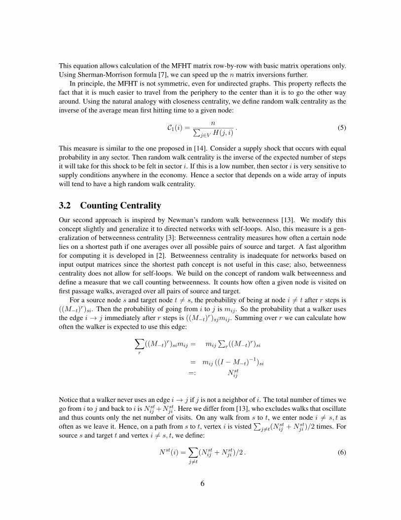
Figure 2: A A small network with a self-loop. B Centrality measure in

In Figure 2 we plot a small network illustrating the differences between our two centrality ap-proaches regarding the role of self-loops. Depending on the self-loop weight a44 either node 3 or 4has the highest counting betweenness in this network. In contrast, independently of a44 node 3 isalways most central with respect to random walk centrality.

4 Central Sectors in Modern EconomiesTable 1 presents the most central sectors in each economy. Our countries are Argentina, Australia,Austria, Belgium, Brazil, Canada, China, the Czech Republic, Denmark, Finland, France, Germanyin 1995 and in 2000, Great Britain, Greece, Hungary, India, Indonesia, Ireland, Israel, Italy, Japan,Korea, Luxembourg, the Netherlands, New Zealand, Norway, Poland, Portugal, the Russian Federa-tion, Slovakia, South Africa, Spain, Sweden, Switzerland, Turkey, Taiwan, and the United States in1995 and in 2000. These countries account for more than 85% of world gross domestic product.

It is striking that “Wholesale and retail trade”is most frequently the sector with highest centrality.In many economies, this sector has the highest share of final demand. Still, it is noteworthy that ournormalization does not depend upon this fact. For example, in Germany in 2000, this sector accountsfor 12% of final demand, but out normalization makes this sector’s entries sum to unity, just like anyothers. Real estate activities is the second most important sector accounting for 9.6% of final demand,but its random walk centrality is ranked only eighth. One can tentatively conclude that high randomwalk centrality is actually based upon a rich pattern of output linkages, not on the sector’s absoluteimportance in the economy.

Counting centrality captures sectors with hig average betweenness and also important self-loops.Focussing on counting centrality reveals the importance of Nokia in Finland and the motor vehiclesector in several advanced industrialized economies. Textiles play an important role in China, In-donesia, and Turkey, showing the importance of that manufacturing sector in a countries with lowwages. Finally, it is worth noting that public administration, defence, and compulsory social securityis most central in Israel, South Africa, and the United States.

8

Table 1: Most Central SectorsCountry Random Walk Centrality Counting Centralityarg1997 Food products Health and social workaus199899 Wholesale and retail trade Wholesale and retail tradeaut2000 Wholesale and retail trade Wholesale and retail tradebel2000 Wholesale and retail trade Motor vehiclesbra2000 Wholesale and retail trade Food productscan2000 Wholesale and retail trade Motor vehiclesche2001 Wholesale and retail trade Chemicals excluding pharmaceuticalschn2000 Construction Textilescze2000 Wholesale and retail trade Constructiondeu1995 Wholesale and retail trade Motor vehiclesdeu2000 Wholesale and retail trade Motor vehiclesdnk2000 Wholesale and retail trade Food productsesp2000 Wholesale and retail trade Constructionfin2000 Wholesale and retail trade Communication equipmentfra2000 Construction Motor vehiclesgbr2000 Wholesale and retail trade Health and social workgrc1999 Wholesale and retail trade Wholesale and retail tradehun2000 Wholesale and retail trade Motor vehiclesidn2000 Wholesale and retail trade Textilesind199899 Land transport Food productsirl2000 Construction Office machineryisr1995 Defence and social security Health and social workita2000 Wholesale and retail trade Wholesale and retail tradejpn2000 Other Business Activities Motor vehicleskor2000 Construction Motor vehicleslux2000 Finance and insurance Finance and insurancenld2000 Wholesale and retail trade Food productsnor2000 Wholesale and retail trade Food productsnzl200203 Wholesale and retail trade Food productspol2000 Wholesale and retail trade Wholesale and retail tradeprt2000 Wholesale and retail trade Health and social workrus2000 Wholesale and retail trade Food productssvk2000 Wholesale and retail trade Motor vehiclesswe2000 Other Business Activities Motor vehiclestur1998 Food products Textilestwn2001 Wholesale and retail trade Office machineryusa1995 Wholesale and retail trade Health and social workusa2000 Defence and social security Defence and social securityzaf2000 Defence and social security Defence and social security

It is impressive to visualize the structure in complicated sets of data by using clustering tech-niques. A clustering assigns a set of objects into groupings according to a measure of similarity. Ournormalized data are of dimension 2209 = 47 ∗ 47, but our focus on centrality reduces each economyto an element in a 47-dimensional space. Reducing the complex networks to a list of centrality val-

9

Belgium

Spain

Austria

Italy

Czech Republic

Poland Slovakia Finland Sweden

United Kingdom

Netherlands

Taiwan

Switzerland

Ireland

Germany1995

Germ

any

Fra

nce

Hun

gary

J

apan

USA1995

USA

Argentina Brazil

Greece Portugal

Australia

Canada

South Africa

Norway

Denmark

nzl

Israel Luxembourg Indonesia

China K

orea

India

Tur

key

Rus

sia

Germ

any1995

Germ

any

France

United Kingdom

Netherlands

Austria Portugal Belgium Italy

Czech Republic

Spain

Poland

Slovakia

Hungary

Japan

USA19

95

USA

A

rgen

tina

Bra

zil South Africa

Australia Canada

Switzerland Ireland

Denmark

nzl

Israel

Greece

Luxembourg

Indonesia

Finland Sweden

Norway China India

Turke

y

Kor

ea

Tai

wan

Rus

sia

A B

Figure 3: Dendrograms of clusterings according to A Random Walk Centrality and B Counting Between-ness

ues, we can dramatically compress the relevant information. Even more, we do not want to attachtoo much importance to the actual centrality numbers themselves. Instead, we are concerned withtheir rankings. Thus, for us two economies are similar if their Spearman rank correlation of centralityacross sectors is high. This also captures the fact that we had to remove sectors without input oroutput to keep our measures well-defined.

Perhaps the easiest and most commonly used clustering method is hierarchical clustering, fora detailed treatment see e.g. [8]. This iterative algorithm groups economies starting with the mostsimilar ones. Our distance measure is Spearman rank correlation. Figure 2 shows that Belgiumand Spain are the two most similar networks; hence, they are the closest two networks. We usecomplete linkage clustering to draw the rest of the dendrogram with respect to a ranking accordingto a betweenness measure: Let A and B be two sets; then distance between them is d(A,B) =max{d(x, y) : x ∈ A, y ∈ B}. The clustering algorithm proceeds iteratively by identifying nearestneighbors and showing their distance using branch heights in the dendrogram. When all the initialsingletons are linked, the algorithm stops. Cutting the tree at a predefined threshold gives a clusteringat the selected precision. For example, at the threshold 0.65, there are three clear clusters in Figure 2:(1) a group of advanced industrial economies ranging from Belgium through the United States; (2) amixed group of countries where agriculture may be important; and (3) a group of rapidly emergingeconomies ranging from China through Russia.

Figure 3b shows a clustering based upon the similarity of networks according to counting central-ity. Taiwan is grouped quite differently in the two clusterings. According to random walk centrality,it is in the middle of the advanced industrial economies. But in the clustering according to countcentrality, it is a close neighbor of Korea, in the “Asian Tigers”sub-group of the emerging economies.

10

An important reason for this different grouping is that Korea and Taiwan have food products andtextiles industries that both have large self-loops. This clustering captures the remnants of the his-torical development process in which both economies were based on manufacturing sectors just onegeneration ago.

It is reassuring that the clusterings are stable across the two measures. The groupings are natural;it is appropriate that the American and German economies, each sampled five years apart, are mostclosely related their former selves. Leontief argued that the stability of input-output relations acrosstime was a good empirical justification for using a fixed-coefficients technology in his original work.These clusterings support his assertion.

Focusing on Random Walk Centrality, we turn briefly to a detailed study of two different pairsof similar economies. Tables 2 and 3 look into the details inherent in the clusterings that arise fromour the Random Walk Centrality. The two nearest neighbors are Belgium and Spain. We report theranks of the ten most central sectors in each country. There are forty-seven sectors in each case, butreporting all would overwhelm the reader. The list of ten sectors shows the level of disaggregation ofour data. The main conclusion drawn from Table 2 is that there is a remarkable similarity between theflow of intermediate inputs in each of these economies. Retail trade and construction are notoriouslypro-cyclical, and Random Walk Centrality shows that fact clearly.

Table 2: Two Similar Advanced EconomiesRank Sector in Belgium Sector in Spain1 Wholesale and retail trade Wholesale and retail trade2 Construction Construction3 Other Business Activities Hotels and restaurants4 Food products Other Business Activities5 Chemicals excluding pharmaceuticals Food products6 Hotels and restaurants Real estate activities7 Travel agencies Travel agencies8 Motor vehicles Other social services9 Agriculture Motor vehicles10 Health and social work Agriculture

India and Turkey cluster together, but they are somewhat less similar than Belgium and Spain;in Fig. 2, the length of the branch that brings them together is twice as high as that for Belgiumand Spain. Food products, construction, and hotels and restaurants all have high centrality rankings.These rankings seem to indicate that the sectoral composition of business cycles is somewhat differ-ent in an emerging economy.

11

Table 3: Two Similar Emerging EconomiesRank Sector in India Sector in Turkey1 Land transport Food products2 Food products Wholesale and retail trade3 Agriculture Construction4 Construction Hotels and restaurants5 Hotels and restaurants Agriculture6 Textiles Finance and insurance7 Health and social work Textiles8 Wholesale and retail trades Land transport9 Chemicals excluding pharmaceuticals Travel agencies10 Electricity Machinery, nec

5 ConclusionWe developed two centrality measures suited for measuring the flow of economic activity betweensectors in an economy. A node’s random walk centrality is the inverse of its mean first hitting time,averaged over all pairs of source and target. In an input-output table a central sector will bear thebrunt of a supply shock very quickly. A node’s counting centrality measures expected number oftimes that a commodity passes though before it exits the system as a good for final demand. Again,we average over all pairs of source and target. The main difference between the two measures is thatcounting centrality captures the effects of self-loops, an important part of economic networks.

We have concentrated on the flow of economic activity across the sectors of the economy. Ournormalization was to divide the input-output table by its row sums. Hence we treated sectors that hadlarge volumes of output of intermediate goods in the same way as those that had small volumes. Wedirected our attention to the flow of economic activities as intermediate outputs before they exited thesystem for use in final demand.

Taking full advantage of the the consistency of the data across countries, we have given the firsthierarchical clusterings of these economic networks. The clusterings were intuitive. They revealedlevel of development and similarity of the same economy across time. To the best of our knowledge,we have given the first hierarchical clusterings of the production structures of different economies.We anticipate that others will build on this aspect of our work.

Using random walk centrality, we interpret a central node as a sector that it is most immediatelyaffected by a random supply shock. Hence, if one could predict sectoral shocks accurately, one wouldshort equity in a central sector and go long equity in a remote sector during an economic downturn.Using counting centrality, we interpret a central sector as one that is both central and has a strongself-loop. This measure of centrality is related to the velocity of money, and it does not ignore thatfirms in the same sector actually buy and sell from each other.

There is a lot more work to be done in this area. The theory of networks has flourished inthe last two decades, and consistent international data has also become widely available during thistime. In the social sciences, network theory arose from theoretical sociology, but it obviously hasready applications to economic data, both real and financial. we expect that our techniques will beuseful for analyzing payment networks and other financial systems. Also, our measure of countingbetweenness is useful for any network where self-loops are important. If the nodes of a social network

12

describe aggregates such as clubs or teams–not just individuals themselves–then self-loops becomean important part of its architecture.

References[1] B. Bollobas. Random graphs. Cambridge Studies in Advanced Mathematics, 2001.

[2] Ulrik Brandes. A Faster Algorithm for Betweenness Centrality. Journal of Mathematical Soci-ology, 25(2):163–177, 2001.

[3] L. C. Freeman. A set of measures of centrality based on betweenness. Sociometry, 40:31–41,1977.

[4] L. C. Freeman. Centrality in social networks: Conceptual clarification ı. Social Networks,1(4):215–239, 1979.

[5] L. C. Freeman, S. P. Borgatti, and D. R White. Centrality in valued graphs: A measure ofbetweenness based on network flow. Social Networks, 13(2):141–154, 1991.

[6] Lothar Krempel Gancho Ganchev and Margarita Shivergeva. How to view structural change:The case of economic transition in bulgaria. Research Project at the Max-Planck Institute forthe Study of Societies: Visualizing Economic Tansition in Bulgaria, July 2001.

[7] G.H. Golub and C.F. Van Loan. Matrix computations. Johns Hopkins University Press, 1996.

[8] T. Hastie, R. Tibshirani, and J. Friedman. The Elements of Statistical Learning. Springer, 2001.

[9] Wassily Leontief. Input-Output Economics (2nd ed.). Oxford University Press, New York,1986.

[10] John B. Long and Charles I. Plosser. Real business cycles. Journal of Political Economy,91:39–69, 1983).

[11] L. Lovasz. Random walks on graphs: a survey. Combinatorics, 2(80):1–46, 1993.

[12] James McNerney. Network properties of economic-input output networks. International Insti-tute for Applied Systems Analysis Interim Repor IR-09-003, January 2009.

[13] M. E. J. Newman. A measure of betweenness centrality based on random walks. Social Net-works, 27(1):39–54, 2005.

[14] Jae Dong Noh and Heiko Rieger. Random walks on complex networks. Phys. Rev. Lett.,92(11):118701, 2004.

13