Which Countries Export FDI, and
44
Which Countries Export FDI, and How Much? ∗ by Assaf Razin, † Yona Rubinstein ‡ Efraim Sadka § November, 2003 ∗ We wish to thank Anil Kashyap, Elhanan Helpman, Gita Gopinath and John Romalis for many useful comments and suggestions. This paper was completed when Rubinstein and Sadka visited Razin at Cornell University. † Tel-Aviv University, Cornell University, CEPR, NBER and CESifo. ‡ Tel-Aviv University § Tel-Aviv University 1 Abstract The paper provides a reconciliation of Lucas’ paradox, based on fixed setup costs of new investments. With such costs, it does not pay a firm to make a “small” investment, even though such an investment is called for by marginal productivity conditions. Using a sample of 45 developed and developing countries we estimate jointly the participation equation (the decision whether to invest at all) and the FDI flow equation (the decision how much to invest). We find that countries which are more likely to serve as source for FDI exports than their characteristics project export lower flow of FDI than is predicted by their characteristics. This negative correlation suggests that the source countries with relatively low setup costs are also those with high marginal productivity of capital. Stanford University John A. and Cynthia Fry Gunn Building 366 Galvez Street | Stanford, CA | 94305-6015
Transcript of Which Countries Export FDI, and
Which Countries Export FDI, and How Much?∗
by
Assaf Razin,†
Yona Rubinstein‡
Efraim Sadka§
November, 2003
∗We wish to thank Anil Kashyap, Elhanan Helpman, Gita Gopinath and John Romalis for many
useful comments and suggestions. This paper was completed when Rubinstein and Sadka visited Razin
at Cornell University.†Tel-Aviv University, Cornell University, CEPR, NBER and CESifo.‡Tel-Aviv University§Tel-Aviv University
1
AbstractThe paper provides a reconciliation of Lucas’ paradox, based on fixed setup costs of new investments. With such costs, it does not pay a firm to make a “small” investment, even though such an investment is called for by marginal productivity conditions. Using a sample of 45 developed and developing countries we estimate jointly the participation equation (the decision whether to invest at all) and the FDI flow equation (the decision how much to invest). We find that countries which are more likely to serve as source for FDI exports than their characteristics project export lower flow of FDI than is predicted by their characteristics. This negative correlation suggests that the source countries with relatively low setup costs are also those with high marginal productivity of capital.
Stanford University John A. and Cynthia Fry Gunn Building
366 Galvez Street | Stanford, CA | 94305-6015

Table A2: Data Source Variables: Source:
Import of Goods Direction of Trade Statistics, IMF FDI Inflows International Direct Investment Database, OECD Unit Value of Manufactured Exports World Economic Outlook, IMF Population International Financial Statistics, IMF GDP World Development Indicators, World Bank Distance Shang Jin Wei’s Website: www.nber.org/~wei Bilateral Telephone Traffic Direction of Traffic: Trends in International
Telephone Tariffs, International Telecommunications Union
Education Attainment Burro-Lee Dataset: www.nber.org/N... Roads ….. Language ….. Longitude and Altitude ….

Table A1: List of Countries, by Observed Source/Host Status
Observed as Country Source1 Host
Argentina + + Australia + + Austria + + Belgium + Brazil + Canada + + Chile + China + Columbia + Denmark + Ecuador + Egypt + Finland + France + + Germany + + Greece + Hong Kong + India + Ireland + Israel + Italy + + Japan + + Korea + Kuwait + Malaysia + Mexico + Netherlands + + New Zealand + Nigeria + Norway + + Peru + Philippines + Portugal + Saudi Arabia + Singapore + South Africa + Spain + Sweden + + Switzerland + Taiwan + Thailand + Turkey +

United Kingdom + + United States + + Venezuala + 1We have information on whether a country is a source country only for OECD countries.

1 Introduction
In an influential paper, Lucas (1990) asks: “Why doesn’t capital flow from rich to poor
countries?” Indeed, the law of diminishing returns implies that the marginal product of
capital is high in poor countries and low in rich countries. Therefore, capital should flow
from rich to the poor countries.
With standard constant-returns-to-scale production functions, when the wage (per
efficiency units of labor) is higher in a rich country than in a poor country, then the
return to capital must be lower in the rich country than in the poor country. Therefore,
the existence of “huge” wage gap between rich and poor countries must be associated
with an opposite gap in the rates of return to capital. Given that labor is not allowed
to freely migrate from poor to rich countries, it follows that capital would flow in the
opposite direction, thereby equaling the returns to capital and concomitantly wages too.
The equalization of wages (indirectly through international capital flows) would eliminate
the need to control migration. In practice, however, this is hardly the case. Even though
barriers to international capital mobility are by and large being eliminated, the wage gap
is still in force, and migration quotas from poor to rich countries have to be enforced.1
Lucas reconciled this paradox by appealing to a human capital externality that gen-
erates a Hicks-neutral productivity advantage for rich countries over poor countries. The
average level of educational attainment is an external factor into the production function,
that raises the productivity of labor, and more importantly, capital. As a result, capital
flows, though equalize the rates of return to capital, fall short of equalizing the capita-
labor ratio. Therefore, wages (per efficiency units) are not equalized. Labor of all skill
levels has still strong incentives to migrate from poor to rich countries.
In this paper we provide yet another reconciliation of Lucas’ paradox, based on fixed
setup costs of new investments. With such costs, it does not pay a firm to make a
“small” investment, even though such an investment is called for by marginal productivity
conditions (that is, the standard first-order conditions for profit maximization). Put it
1Note also that despite the expansion of international trade in goods, still the Stolper-Samuelson
(1941) factor price equalization theorem does not manage to eliminate the wage gap.
2

differently, the firm’s investment decision is twofold now: marginal productivity conditions
determine how much to invest, whereas a “participation” condition determines whether
to invest at all. In such a framework, the Lucas paradox can be reconciled: rates of
return to capital are equalized and concomitantly the wage gap remains in force.
When one looks at data on gross international capital flows of foreign direct investment
(FDI), one is immediately struck by the lack of flows from many rich countries to many
host countries. We looked at data on bilateral FDI flows in a sample of 45 countries,
both developing and developed, over the period of years from 1981 to 1998. Out of 45 x
44 = 1980 source-host pairs of countries with potential bilateral FDI flows, we found that
the number of pairs with actual flows is only 334! There were only 12 countries that made
any FDI export over that period and most of these countries exported FDI to only one
other country. These crude findings provide a prima facia suggestion for the existence
of fixed setup costs of investment that nullify the potential of “small” capital flows that
may have been called for by marginal productivity conditions.
We emphasize again that whether a cell of s−h pair becomes active or inactive and howmuch flow is recorded in this cell in case it becomes active are jointly and simultaneously
determined. Thus, the selection of pairs of countries into active and inactive cells is not
exogenous. If one treats this selection as exogenous, the estimates of the determinants
of FDI flows are biased. We therefore employ a Heckman selection-bias method in order
to simultaneously estimate the determinants of FDI flows and the selection of countries
into pairs of s− h countries.2
The organization of the paper is as follows. Section 2 explains the way Lucas reconciles
the paradox of the inadequacy of capital flows from rich to poor countries. Section 3
presents our model of fixed setup costs of investment. This model is used in Section
4 to provide an alternative reconciliation of Lucas’ paradox. Section 5 presents the
econometric approach. The data are described in Section 6. A crude examination of
the potential for selection bias in the data is done in Section 7. Simultaneous estimation
results of the determinants of FDI flows and whether they are formed at all are presented
2See Heckman (1979).
3

in Section 8. The results are interpreted and conclusions are drawn in Section 9. Section
10 concludes.
2 Lucas’ Reconciliation of the Paradox
The law of diminishing returns implies that the marginal product of capital is high in poor
countries and low in rich countries. Therefore, capital should flow from rich to the poor
countries. But, it is hard to account in reality for any significant income-equalizing capital
flows. Addressing the question: “Why doesn’t capital flow from rich to poor countries?”,
Lucas (1990) employs a standard constant-returns-to-scale production function:
Y = AF (K,L), (1)
where Y is output, K is capital and L is effective labor. The latter is used in order
to allow for differences in the human capital content of labor between developed and
developing countries. The parameter A is a productivity index which may reflect the
average level of human capital in the country, external to the firm as in Lucas (1990). In
addition, A may reflect the stock of public capital (roads and other infrastructure) that
is external to the firm. In per effective-labor terms, we have:
y ≡ Y/L = AF (K/L, 1) ≡ Af(k). (2)
The return to capital is:
r = Af 0(k), (3)
whereas the wage per effective unit of labor is:
w = A[f(k)− kf 0(k)]. (4)
Let a variable with an asterisk (∗) stand for a rich (developed) country and a variablewithout an asterisk for a poor (developing) country. The function f is common to all
4
countries. Initially, r∗0 < r0. But when capital can freely move from rich to poor countries,
then rates of return are equalized, so that:
r∗ = A∗f∗0(k∗) = Af 0(k) = r. (5)
Lucas (1990) essentially assumes thatA∗ > A (because of a human-capital externality).
Hence, it follows from equation (5) that k∗ > k (because of a diminishing marginal product
of capital). Therefore, employing equation (4) it follows that w∗ > ω.
That is, at equilibrium, workers can earn higher wages (per effective labor) in the
rich country than in the poor country, and administrative means (migration quotas) are
employed to impede the flow of labor from poor to rich countries. Yet there is no pressure
on capital to flow in the opposite direction because rates-of-return on capital are equalized.
Note that with A = A∗, one cannot explain the puzzle posed by Lucas (1990), which is
the existence of a pressure on labor to move from poor countries to rich countries without
the existence at the same time of a pressure on capital to flow in the opposite direction.
The next section provides another explanation for this puzzle.
3 Lumpy Adjustment Cost of Investment
We employ a “lumpy” adjustment cost for new investment, in the form of a fixed setup
cost of investment. This specification, which has been recently supported empirically by
Caballero and Engel (1999, 2000), creates economies of scale in investment.3
Consider a two-period economy with a single, all-purpose good. In the first period
there exists a continuum of N firms which differ from each other by a productivity index
ε. We denote a firm which has a productivity index of ε by an ε−firm. The cumulativedistribution function of ε is denoted by G(·), with a density function g(·).
3Economies of scale either in the production or investment technologies are also a key contributor to
the gains from trade and economic integration. For example, based on estimates taken from a partial equi-
librium analysis, the Cecchini (1988) Report assessed that the gains from taking advantage of economies
of scale will constitute about 30 percent of the total gains from the European market integration in 1992.
5

We denote the initial net capital stock of each firm by (1−δ)K0. This consists of the net
initial stock, K0, of the preceding period, multiplied by one minus the depreciation rate, δ.
If an ε−firm invests I in the first period, it augments its capital stock toK = (1−δ)K0+I
and its gross output in the second period will be AF (K,L)(1 + ε), where L is the labor
input (in effective units). Naturally, ε ≥ −1 so that G(−1) = 0.We assume that there exists a fixed setup cost of investment, C, which is the same for
all firms (that is, independent of ε). If an ε−firm invests in the first period an amount
I = K−(1−δ)K0 in order to augment its stock of capital toK, its present value becomes:
V +(ε;K,L) =F (K,L)(1 + ε)− wL+ (1− δ)K
1 + r− [K − (1− δ)K0 + C].
This firm chooses K and L in order to maximize its value. The first-order conditions
FK(K,L)(1 + ε) = r + δ (6)
and
FL(K,L)(1 + ε) = w (7)
define the optimal K and L for an ε−firm, if it chooses to make a new investment atall. These are denoted by K+(ε;w, r) and L+(ε;w, r), respectively. Note, however, that
an ε−firm may chose not to invest at all [that is, to stick to its existing stock of capital
(1 − δ)K0)] and avoid the setup lumpy cost C. In this case its labor input, denoted by
L−(ε;K0;w, r) is defined by:
FL[(1− δ)K0, L](1 + ε) = w. (8)
Note that L− depends on the initial stock of capital. Naturally, low ε−firms may not findit worthwhile to incur the setup cost C. In this case its present value is:
V −[ε; (1−δ)K0, L−(ε;K0, w, r)] = {F [(1−δ)K0, L
−(ε;K0;w, r)](1+ε)−wL+(1−δ)K20}/(1+r).(9)
6

Therefore, there exists a cutoff level of ε, denoted by ε0, such that an ε−firm will make anew investment if and only if ε > ε0. This cutoff level of ε depends on K0, w and r. We
write it as ε0(K0;w, r) and define it by:
V +©ε0(K0;w, r);K
+ [ε0(K0;w, r);w, r] , L+[ε0(K0;w, r);w, r]
ª(10)
= V −©ε0(K0;w, r); (1− δ)K0, L
−[ε0(K0;w, r);K0;w, r]ª.
We continue to assume that labor is confined within national borders. Denoting the
country’s endowment of labor in effective units by L̃0, we have the following labor market
clearance equation:
N
ε0(K0;w,r)Z−1
L−[ε;K0, w, r]g(ε)dε+N
ε̄Zε0(K0;w,r)
L+(ε;w, r)g(ε)dε = L̃0,
where ε̄ is the upper productivity level. Dividing the latter equation through by N, yields:
ε0(K0;w,r)Z−1
L−[ε;K0;w, r]g(ε)dε+
ε̄Zε0(K0;w,r)
L+[ε;K, r]g(ε) = L0, (11)
where L0 ≡ L̃0/N is the effective labor per firm.
Note that no similar market clearance equation is specified for capital, as we continue
to assume that capital is freely mobile internationally and its rate of return is equalized
internationally.
4 An Alternative Reconciliation of the Paradox
Let us focus on the international differences in the abundance of effective labor relative
to the number of firms, that is, L0. We therefore assume at this stage that K0 = K∗0 and
C = C∗. Naturally, effective labor per firm is more abundant in the developing country.
That is, we assume that:
L̃0/N ≡ L0 > L∗0 ≡ L̃∗0/N∗. (12)
7
We demonstrate that in this case that even though r = r∗ (by the capital mobility
assumption), we nevertheless have w < ω∗. That is, labor wishes to migrate from poor to
rich countries even though capital moves freely from rich to poor countries.
To see this, suppose, on the contrary, that w = w∗. Then the demand for effective
labor of an ε−firm is the same in both countries:
L−(ε;K0;w, r) = L−(ε;K∗0 ;w
∗, r∗)
for the non-investing firms and:
L+(ε;w, r) = L+(ε;w∗, r∗)
for the investing firms. Furthermore, the cutoff productivity level is the same in both
countries:
ε0(K0;w, r) = ε0(K∗0 ;w
∗, r∗).
Hence, the demand for effective labor (per firm) is the same in both countries. There-
fore, this cannot be an equilibrium because the supply of effective labor (per firm) is
higher in the poor country. Thus, at equilibrium, the wage per effective unit of labor
must be lower in the poor country than in the rich country.
It also follows that the higher wage in the rich country reduces the profit from invest-
ment and therefore the cutoff productivity level is also higher in the rich country:
ε0(K0;w, r) < ε0(K∗0 ;w
∗, r∗). (13)
(Recall that K0 = K∗0 and r = r∗.)
In fact, the wage differential must be high enough so as to push ε0(K∗0 ;w
∗, r∗) all the
way to the upper bound ε̄.4 That is, no firm in the rich country makes new investment. To
see this, note that for the investing firms, the capital-labor ratio is governed by equation
4Evidently, if capital mobility is not as perfect as in the model, the rich country will continue to make
new investment (that is, ε∗0 < ε̄).
8

(6). (Recall that with constant returns-to-scale, FK depends on K/L only). Thus, with
r = r∗, the capital-labor ratio for the investing ε−firmmust be the same in both countries.But then equation (7) implies that the wage (per an effective unit of labor) must be the
same in both countries, in contradiction to our conclusion that w < w∗.
To complete the picture, we briefly discuss also international differences in the setup
cost (C). It is plausible that the setup cost is higher in poor countries than in rich countries.
This is because the setup cost may reflect the level of public capital (transportation
infrastructure, communication infrastructure, etc.) and the average level of human capital
[as in Lucas (1990)]. The higher setup cost in the poor country induces fewer firms to
make new investment (that is ε0 shifts to the right). This exerts a further pressure down
on wages in poor countries (and attracts less capital from rich countries).
Consider now the possibility of establishing a new firm. Suppose that the newcomer
entrepreneur does not know in advance the productivity factor (ε) of the potential firm.
She therefore takes G(·) as the probability distribution of the productivity factor of thenew firm. The expected value of the new firm is therefore the maximized value (over K
and L) of:
V̄ (w, r) ≡Z ε̄
−1max
½max{K,L}
·F (K,L)(1 + ε)− wL+ (1− δ)K
1 + r− C −K
¸, 0
¾g(ε)dε,
where C is the setup cost of establishing a new firm and that ε is revealed to the firm
before it decide whether or not to make new investment. The lower wage (per effective
labor) in the poor country makes the expected value of a new firm higher. Therefore:
V̄ (w∗, r∗) < V̄ (w, r).
(Recall that r = r∗.) Thus, the poor country attracts more new firms. Assuming that
newcomer entrepreneurs evolve gradually over time, eventually this process may end up
with full factor price equalization. Naturally, the capital-labor ratios and L ≡ L̃/N
are equalized in this long-run steady state. All this happens even though labor is not
internationally mobile. The establishment of new firms in the global economy may be
9
an engine for FDI flows by multinationals, due to setup-cost advantage over domestic
investors in the host country.
Generally speaking, firms will enter so that in the long-run equilibrium the number of
workers per firm will be the same in both countries, and so will be the capital stock per
worker. During the transition to this long-run equilibrium, wages remain unequal and
FDI flows from the rich country to the poor country.
Our two-country model, which generates capital flows from the rich to the poor coun-
try, can be extended in two ways. First, by assuming more than one industry, each country
may have a setup-cost advantage in a different industry. Consequently, we can have two-
way FDI flows. Second, we may also consider an n-country model which gives rise to
n (n− 1) potential bilateral flows.5 We look at FDI because: (i) this form of internationalflow is assuming a dominant role among all other forms of international flows in recent
years; (ii) fixed setup costs are most pronounced in the case of FDI.
5 The Econometric Approach
The proceeding section presents a model of capital mobility distinguished by setup costs
of investment. In the model an important vehicle, through which capital flows from one
country to another, is foreign direct investment (hereafter: FDI), taking place either in
order to acquire existing firms and investing in them (Mergers and Acquisitions FDI), or
to establish new firms (Greenfield Investment FDI). Our empirical investigation is in the
tradition of the often used gravity models,6 with our adjustments for a selection bias into
5Helpman, Melitz and Yeaple (2003) pose the question of how a source country can simultaneously
make both FDI and exports to the same host country. Their answer rests on productivity heterogeneity
within the source country, and differences in the setup costs associated with FDI and exports. Their
explanation is thus geared toward firm-level decisions on exports and FDI in the source country.6Gravity models postulate that bilateral international flows (goods, FDI, etc.) between any two
economies are positively related to the size of the two economies (e.g., population, GDP), and negatively
to the distance (physical or other such as tariff barriers, information asymmetries, etc.) between them.
For instance, using population as the size variable, Loungani, Mody and Razin (2002) find that imports
are less than proportionately related to the host country population, while they are close to propor-
10

source and host countries. With n countries in the sample, there are potentially n(n−1)pairs of source-host (s−h) countries. In fact, as we show in the data section below, that
the actual number of s−h pairs is much smaller, less than thirty percent of the potential
number. Therefore, the selection into s−h pairs, which is naturally endogenous, cannot
be ignored; that is, this selection cannot be taken as exogenous, which is the standard
practice in most gravity models.
Denote by Yi,j,t the flow of FDI from source country i to host country j in period t.
FDI flows from source country j to host country i are denoted by Yj,i,t. Note that with
this notation, Yi,j,t is always non-negative. But, it may well be zero, because typically,
in a global economy, there are only a few countries which significantly export FDI.
The existence of a setup cost of investment makes investment “lumpy”. This means
that the conventional determinants of FDI flows (such as rate of returns differentials)
have to be strong enough in order to generate a large FDI flow that surpasses a certain
threshold. Otherwise, the observed FDI flow is practically zero. We argue that the sub-
sample of FDI source countries is not a random sample of the countries global economy,
if setup costs play a significant role in the determination of FDI flows. We now develop
a simple econometric approach to study the effect of setup costs and correct for selection
bias in the analysis of FDI flows.7
tionately related to the source country population. Correspondingly, FDI flows increase by more than
proportionately with both the source and the host-country populations.7Correction for selection bias is rare in international economics literature. A notable exposition is
Broner, Lorenzoni and Schmukler (2003) who applied the Heckman selection model in estimating the
average maturity of sovereign debt. They take into account the incidental truncation of the data, since
the average maturity is available only for countries which issue bonds to the world market. The missing
observations cannot be treated as zero maturity. They show, as expected, that countries with weak macro
economic stance are less likely to issue bonds. In this case the problem reduces to be the standard Tobin
model.
11

5.1 FDI Flows and the “Participation" Equation
To simplify, but without losing generality, let us assume that, in a world with no setup
costs, potential FDI flows exhibit the following linear form:
Yi,j,t = Xi,j,tβ + Ui,j,t, (14)
whereXi,j,t stands for a vector of observed variables, such as per-capita income differentials
between country i and country j (reflecting differences in the capital-labor ratio) that
potentially can explain the pattern of FDI flows, excluding the effect of setup costs. The
vector β is the ceteris paribus effect of Xi,j,t on Yj,i,t. The error term Ui,j,t, is a composite
of (i) an unobserved time-invariant heterogeneity factor (θi,j) , and (ii) a i.i.d. random
shock term which is i-j pairwise-specific¡ηi,j,t
¢, reflecting fluctuations in macroeconomic
policy, political events, etc., that are unique to the i-j pair. That is:
Ui,j,t = θi,j + ηi,j,t, (15)
Let Zi,j,t be a latent variable, indicating the maximized profit (hereafter: π) from the
direct investment made in host country j, by a firm in the source country i , in period t.
Following our model we allow Zi,j,t to be determined by setup costs (Ci,j + ci,j,t),
in addition to Xi,j,t and¡ηi,j,t
¢. Note that the setup costs consist of two elements: (a)
time- invariant costs (Ci,j), reflecting persistent features of the i−j pair, such as language,geographical distance etc., and (b) time-variant setup costs (ci,j,t), such as communication
and transportation costs. We assume that the vector Zi,j,t, as a function of Xi,j,t, exhibits
the following linear form:
Zi,j,t = Xi,j,tα+ Vi,j,t, (16)
where the vector α is the ceteris paribus effect of Xi,j,t on Zi,j,t. Note that in the case
where Xi,j,t affects the value of maximized profit, the same way as it influences Yi,j,t in
equation (14) , then α = β. The error term Vi,j,t , in the profit equation, is a composite of
(i) the unobserved setup costs (Ci,j + ci,j,t) and (ii) the pairwise-specific π shocks (νi,j,t):
Vi,j,t = −Ci,j (θi,j) + νi,j,t, (17)
12
where νi,j,t = ηi,j,t − ci,j,t. We further assume that, for a random sample, the classical
assumptions regarding the error term do hold. In particular, we assume that:8
E (Ui,j,t | Xi,j,t) = E (Ui,j,t) = 0 (18)
and
E (Vi,j,t | Xi,j,t) = E (Vi,j,t) = 0
It follows from equation (15) and equation (17) that:
cov (Ui,j,t, Vi,j,t) > 0. (19)
Now, according to our model, FDI flows (Yi,j,t) are positive, if and only if Zi,j,t > 0.
Denote by
Di,j,t =
1 if Zi,j,t > 0
0 otherwise.
(20)
Note that whereas Zi,j,t is not observed, the binary variable Di,j,t is indeed observed .
The fundamental parameters of interest in our analysis are β and Ci,j.
5.2 Setup Costs and Selection Bias
The population regression function for Equation (14) is:
E (Yi,j,t | Xi,j,t) = Xi,j,tβ (21)
Many previous studies aimed at estimating the effects of X on Y in the context of
international capital mobility (and also, similarly, in the context of goods mobility through
international trade) typically ignore the effect of unobserved setup costs on the observed
capital flows. However, the regression function for the sub-sample of countries, for which
we do indeed observe positive FDI flows is :
E (Yi,j,t | Xi,j,t, Di,j,t = 1) = Xi,j,tβ +E (Ui,j,t | Xi,j,t, Di,j,t = 1) (22)
8At this stage we ignore serial correlation in the error terms.
13
Note that the last term is no longer equal to zero. Furthermore, the termE (Ui,j,t | Xi,j,t, Di,j,t = 1)dep
on Xi,j,t, unlike the classical assumptions concerning regression functions applied to ran-
dom samples.
To see this more clearly, one can substitute equations (15) and (20)into (22) , to get:
E (Yi,j,t | Xi,j,t, Di,j,t = 1) = Xi,j,tβ+E [(θi,j + εi,j,t) | Xi,j,t, (−Ci,j − ci,j,t + εi,j,t) > −Xi,j,tα]
(23)
Now, one can verify directly from Equation (23) that the OLS estimator for β is indeed
biased.
Figure 1 provides the intuition. Suppose, for instance, that Xi,j,t measures the per-
capita income differential between the ith source country and the jth potential host coun-
try, holding all other variables constant, namely per-capita income differentials between
the ith source country and all the rest of the countries. Our theory predicts that parame-
ter β is positive in this case. This is shown by the upward sloping line AB. Note that this
slope is an estimate of the “true” underlying effect of Xi,j,t on Yi,j,t. But, recall that flows
could be equal to zero if the set up cost are sufficiently high. The capital-flow threshold
derived from the setup costs is shown as line TT’ in Figure 1.
However, recall that the data include only those country pairs for which Yi,j,t is positive.
This sub-sample is, therefore, no longer random . Moreover, as Equation (23) makes clear
the selection of country pairs into this sub-sample depends on the vector Xi,j,t.
To see this, suppose, for instance, that for high values of Xi,j,t (the specific level XH in
Figure 1) i-j pair-wise FDI flows are all positive. That is, for all pairs of countries potential
Yi,j,t are higher than the threshold line. Thus, the observed average, for Xi,j,t = XH is
also equal to the conditional population average, point R on the line AB. However, this
does not hold for low values of Xi,j,t (denoted by XL). For those i-j pairs we observe
positive values of Yi,j,t only in a non-random sample of the population. For instance,
point S is excluded from the observed sub-sample of positive FDI flows. consequently, as
predicted by our model, we observe only those with low setup cost (namely high Vi,j,t),
among those with low Xi,j,t .As seen in Figure 1, the observed conditional average is at
point M0, which lies above point M. The sub-sample OLS regression line is shown by the
14

line A0B
0, which understates the influence of the income per capita differentials on the
flows of FDI.
To overcome the selection bias we employ a variation of the standard Heckman’s
selection model (Heckman (1979)) extended to the analysis of panel data (Kyriazidou
(1996)). In the first stage we use a Probit analysis to estimate the Participation Equation,
namely the likelihood of having positive FDI flows in our sample. In the second stage,
we use estimates of unobserved set up costs are used to correct for selection bias in the
estimates of the effect of the per-capita income differentials on FDI flows.
As standard in the literature, we assume that the i-j pairwise-specific errors (νi,j,t) in
the π equation are distributed normally. That is:
νi,j,t ∼ N¡0, σ2
¢. (24)
Then, the probability of surpassing the FDI-flow threshold (for the Probit) exhibits the
following form:
Pr(Di,j,t = 1 | ·) = Φ (Xi,j,tα+ δi,jFi,j) , (25)
where
Fi,j =
1 if i is the source country and j is the host country
0 otherwise
We estimate Equation (25) by controlling for fixed-effects. Finally, the vector of estimated
fixed-effects (δi,j) , from the Probit model, yields an unbiased estimator vector for the
time-invariant element of the setup costs (Ci,j). Having these estimates, we get unbiased
estimates of β, as well.
Figure 2 provides an intuition for our econometric strategy to back up estimates for
the time invariant setup costs. On the horizontal axis we plot the error term in the π
equation (νi,j,t −Xi,j,tα). According to our model, there is a positive FDI flow from a
source country i to a host country j, if and only if, Xi,j,tα − Ci,j − νi,j,t > 0. For both
high and low values of Ci,j , there is a positive probability of observing FDI flows from
source country i to host country j . However, the likelihood to observe a positive flow
for high Ci,j
¡CHi,j
¢is lower than the likelihood for a medium-small Ci,j
¡CMi,j
¢. Therefore,
15

assuming that the stochastic properties of νi,j,t do not vary over time ( in particular no
serial correlation), it follows that the frequency of positive FDI flows between country pairs
associated with CHi,j is lower than the corresponding frequency associated with country
pairs with CMi,j . Therefore, there exists a mapping from Ci,j to the average Di,j,t (average
over t) which can be used for estimating the time-invariant setup costs.
Summing up, our econometric approach yields unbiased estimates of two classes of
determinants of FDI flows: (1) the effect of income per-capita differentials on FDI flows,
and (2) the effect of setup costs on FDI flows.
6 Data
Our data is drawn from a sample of 45 countries, both developing and developed countries,
over the period from 1961 to 1998. The data on FDI flows are for the period from 1981 to
1998 only. The FDI data are based on the OECD reports of FDI exports from 12 OECD
source countries to 45 OECD and non-OECD countries. To the best of our knowledge,
the only countries in our sample which do exports FDI but we miss these data are Taiwan
and Hong-Kong. We handle this issue in section 9.
We employ 3-year averages, so that we have six periods (each consisting of 3 years).
The main variables we employ are: (1) standard country characteristics such as GDP or
GDP per-capita, population, educational attainment, geographical longitude and altitude,
language, road length per country’s area, telephone lines per-capita, etc.; (2) s−h pair datasuch as s−h FDI flows, geographical distance, common language (zero-one variable), s−hflows of goods, bilateral telephone traffic, etc. The appendix provides more information
on the data: Table A1 describes the list of the 45 countries in the sample and whether
observed in the sample (at least once) as a source or host country; Table A2 describes the
sources for our data. It is worth emphasizing again that though we have 45 countries in
the sample and potentially 45 x 44 = 1980 s− h pairs (for each of the six periods in the
sample), there are only 540 s− h pairs (12 source countries and 45 host countries) with
positive flows.
16
7 A First Look at the Selection Bias Problem in the
Data
As was already pointed out, the selection of countries into s− h pairs is a key feature in
the data. Out of 1980 potential s− h pairs, we observe only 540 s− h pairs in the data
over a long period of years from 1981 - 1998. Therefore, in this section we take a first
look into the s− h selection pattern.
Consider first the sample of actual observations consisting of 540 s−h pairs, 12 sourceand 45 host countries. This sample exhibits an asymmetry in the (relatively small)
number of source countries and (relatively large) number of host countries. Moreover,
in this self-selected sample, not every source country exports FDI to all host countries.
Do all host countries import FDI from all source countries? This question is answered
in Figure 3, which depict the fraction of host countries that import FDI from x source
countries, x = 1, 2, ..., 12. If the answer is in the positive, then we should find just one
column equalling 45 for x = 12 and all other 11 columns being of zero height. But as
Figure 3 suggests, only 9 of the 45 host countries import FDI from all 12 source countries.
Similarly, Figure 4 depicts the fraction of source countries that export FDI to x host
countries, x = 0, 1, ..., 45. The figure suggests that no source country exports FDI to all
host countries. Furthermore, most source countries export to just one host country.
Given the selection of source and host countries, we next examine whether the number
of host countries each source country exports to and similarly the number of source
countries each host country imports from are random or depend on country characteristics.
Figure 5 illustrates the role of GDP per capita in host countries. The 45 host countries are
classified into (at most) twelve groups along the vertical axis, according to the number of
source countries from which they import FDI. For each such group of host countries, the
average GDP per-capita is depicted along the horizontal axis. The figure shows that the
higher the per-capita GDP in a host country, the larger is the number of source countries
it imports from. A similar pattern is found with respect to educational attainment: the
higher the level of educational attainment in a host country, the larger is the number of
17

source countries it imports from; see Figure 6. No such pattern is found with respect to
the characteristics of the source countries. The twelve source countries are classified into
(at most) 12 categories, according to the number of host countries they export to. (Each
category is a number between 1 and 45.) The average GDP per-capita and the average
educational attainment of the source countries in that category does not seem to affect
the number of host countries in each category; see Figure 7 and 8.
8 Estimation
The dependent variable in all the gravity equations is the log of the FDI flows, deflated
by unit value of manufactured exports.
As a benchmark, we simply estimate the gravity equation (14) as is. That is: (1) we
employ only actually observed s− h pairs, namely we employ the subset of 540 pairs (for
each of the six periods in the sample); (2) we ignore the “participation” equation (25)
which explains the endogenous selection of s− h matches, namely “zeros” were inserted
into the no-flow cells among the 540 cells. The rationale for inserting “zeros” is as follows.
Generally, when one observes no FDI flows between a pair of countries, it could be either
because the two countries do not wish to have such flows even in the absence of fixed cost
or because setup costs are prohibitive for low flows. But in the benchmark case which
ignores setup costs, cells with no FDI flows “truly” indicate zero flows. This is why we
assume a one-dollar value (with the log equalling zero) as a common low value for the
value of the FDI flows in the no-flow cells. (All other positive flows have logarithmic value
much exceeding zero.9)
The estimation results for this benchmark case are described in panel A of Table 1.
We make three alternative specifications (I, II, III). The difference between the first two
specifications is that the first one has GDP as one of the size (gravity) variables, whereas
in the second one population is the size variable. Specification II includes also GDP
9We performed robustness tests by replacing the zeros by large negative numbers. The conclusions
are not meaningfully changed.
18

per-capita as an explanatory variable. Two findings clearly emerge: first, the coefficients
(elasticities) of the GDP variable (in the first specification) in both the host and source
country and the GDP per-capita (in the second specification) in both the host and source
country are positive and significant. Second, the elasticity is significantly larger for the
source country. We also find that countries that share a common language has signifi-
cantly more (50%) FDI flows between them than countries that do not share a common
language. Likewise, the coefficient of distance is negative and significant. Specification
III employs source/host ratios of GDP per-capita, population and educational attainment.
Contrary to the premise that capital flows from rich to poor countries, the coefficient of
GDP per-capita ratio is negative and very significant with this specification. Likewise,
contrary to Lucas’ explanation, the coefficient of the ratio of educational attainment is
insignificant.
The benchmark case treats the selection of the 540 s− h pairs as exogeneous. That
is, it ignores the fact that 33 countries in the sample of 45 countries may have not chosen
to export FDI because of economic factors. In addition, the benchmark case ignores the
role that setup costs may have played in generating no-flow pairs: both by reducing the
number of source countries to 12, and by causing some zero flows from the remaining 12
countries. We now study in two stages the role of setup costs in the sample selection
of countries into s − h pairs. We first expand the sample to include all 1980 potential
s− h pairs. At this stage, we still ignore setup costs and insert a low common value for
the log of the FDI flow (namely, zero) in the no-flow cells. The findings are presented
in panel B of Table 1. The characteristics of the host countries drastically lose their
explanatory power. For example, the elasticity of FDI with respect to GDP in the
host country (Specification I) drops from 0.727 to 0.207. Likewise, the coefficient of the
variable of educational attainment in the host country drops from 0.153 to 0.045. The
relevance of the source country characteristics declines too but not as much as that of the
host country characteristics. Therefore, the source country characteristics become more
important relatively to the host country characteristics. FDI flows between countries
with a common language, which were 50% more than between other countries in the
19

benchmark case, are now only 22% higher. Similar findings are found in Specification
III.
This first stage corrects the anomaly found in the benchmark case in Specification III:
now the coefficient of source-host GDP per-capita ratio is positive and significant; namely,
capital flows from rich to poor countries. In addition, the source-host educational attain-
ment ratio becomes significantly positive in line with Lucas’ hypothesis. Nevertheless,
the coefficient of the common language variable is paradoxically negative and significant.
Finally, the complete picture and especially the role played by the unobserved setup
costs are brought to the limelights in the second stage. We do this by jointly estimating
the maximum likelihood of the gravity equation (14) for the full sample of 1980 s−h pairsand the participation equation (25), which arises because of the existence of setup costs.
The unbiased estimates of the coefficients of the gravity equation are presented in panel
A of Table 2. The coefficient of GDP per-capita of the source country (Specification
II), which was positive and significant both in the benchmark case and in the first stage,
becomes now in the full economic model negligible and insignificant. On the other hand,
the effect of the level of educational attainment in the source country is now twice as
large as in either the benchmark case or the first stage. Likewise, the magnitude of the
effect of common language more than doubles relative to either the benchmark case or
the first stage. A similar increase is observed for the distance variable. The effect of the
source-host GDP per-capita ratio (Specification III) disappears now, whereas the effect
of the source-host educational attainment ratio tripled in size.
The estimation results for the participation equation are reported in panel B of Table
2. Unlike in the gravity equation, the magnitude of the effect of GDP per-capita in
the source country (Specification II) is now almost ten times as high as that of the host
country. Furthermore, the effect of the educational attainment in the source country is
barely significant. Also, the common language variable is insignificant, but the coefficient
of the distance variable is negative and significant. Notice that the correlation between
the error terms in the gravity and participation equations (ρ) is negative and significant.
This means that if the actual probability of a pair of countries to be a source-host pair is
20
larger than what is predicted for this pair by the participation equation, then the actual
FDI flow between this pair of countries is smaller than what is predicted by the gravity
equation.
9 Robustness for some missing FDI export data
So far our results are derived from the full sample of countries. As we have already pointed
out, the FDI data are based on the OECD reports of FDI exports from 12 OECD source
countries to 45 OECD and non-OECD countries. The fact that only 12 countries in our
sample serve as source for FDI export may reflect miss-reporting problems rather than
zero FDI exports.
To guard against the possibility that the results presented in section 9 reflect miss-
reporting we re-estimate the model using the sub-sample of only the countries for which
we have FDI export data. This sub-sample contains 12 OECD FDI exporting countries.
We report our findings in Table 3 and Table 4. As both tables make clear, our findings,
concerning the role of country characteristics and h − s pair characteristics, in both the
gravity and the participation equation, hold for this sub-sample as well.
10 Interpretation
The finding that there is a significant correlation (ρ ) between the error terms in the gravity
and participation equations indicates that the formation of an s−h pair of countries and
the size of the FDI flow between this pair of countries are not independent processes.
Furthermore, being negative, this correlation is consistent with the hypothesis of setup
costs of investment. If the setup cost of forming a certain s − h pair of countries is
high, it is less likely for one to observe the formation of this pair. The error term
in the participation equation is thus negative. But then the error term in the gravity
equation is positive. The unobserved heterogeneity in the gravity equation is affected
only by the marginal productivity of capital. However, the unobserved heterogeneity in
21
the participation equation is affected both by the marginal productivity of capital and
by the setup costs of investment. The negative correlation implies that source countries
with low setup costs (and, therefore, with positive "errors" in the participation equation)
are also source countries with high marginal productivity of capital (and, therefore, with
negative "errors" in the gravity equation). Indeed, when we control for source and host
country fixed-effect, the error terms turn to be positively correlated. In other words, once
the invariant unobserved heterogeneity is taken into account we find the more a country
is likely to become a source for FDI exports, the more FDI exports do flow from this
country.
The benchmark case, which ignores the self-selection problem, provides no evidence
for the commonly held view that capital flows from rich to poor countries, because the
elasticity of FDI flow with respect to GDP per-capita in the host country was at least
as high as that in the source country. Also, the benchmark case provides no evidence
for Lucas hypothesis. In one case (Specification I and II) the elasticity of FDI flow with
respect to educational attainment in the source country was positive and about equal to
that in the host country. (Lucas’ hypothesis suggests that this elasticity should be negative
for the source country and positive for the host country). In another case (Specification
III), the coefficient of the ratio of source-host educational attainment was not significantly
different from zero. After correcting for the selection bias in the benchmark case, the
coefficient of the ratio of source-host educational attainment (Specification III) is positive
and significant.
If education, as measured by the average years of schooling is indeed a “good" measure
for cross-countries differences in human capital then these findings are consistent with
Lucas’ hypothesis, however in a subtle way. On the one hand, in agreement with the
Lucas’ hypothesis, the higher the average years of schooling in a host country is, the more
FDI exports flow into this country. On the other hand, it is worth noticing the it does not
hold for the direction of trade. The higher the average years of schooling in a (potential)
source country is the more likely this country is to export FDI flows. Hence, while FDI
exports flow from educated into less educated countries, the higher the education level is
22

the more FDI exports flow into the host countries.
11 Conclusion
The existence of setup costs of investment presents the firm with a twofold investment
decision: whether to invest at all and how much to invest. Therefore, we estimate jointly
a participation equation (the decision whether to invest at all) and a gravity equation
(the decision how much to invest). We find that the error terms in these two equations
are negatively and significantly correlated. The negative correlation suggests that source
countries with relatively low setup costs are also those with high marginal productivity
of capital. Indeed, controlling for source and host countries fixed (country) effect, the
correlation between these errors terms turns out to be in fact positive. These findings
provide supportive evidence for the existence and importance of setup costs of investment
and especially to the different effects on the FDI flows of the marginal productivity and
the setup costs conditions. We find that GDP per-capita differences between source and
host countries are a significant determinant of the decision of whether to invest at all,
but only marginal for the determination of the size of FDI flows. This suggests that
capital does flow from rich to poor countries, but in a more subtle way than what may
be inferred from the marginal productivity conditions. The evidence for the importance
of setup costs of investment, and the subtle way in which the flow of capital from rich to
poor countries, are consistent with our alternative reconciliation of the Lucas’ Paradox.
23
References
[1] Broner, Fernando, A., Guido Lorenzoni, and Sergio L. Schmukler, (2003),
”Why Do Emerging Markets Borrow Short Term?” Princeton University,
http://www.princeton.edu/~guido/shortterm.pdf , July.
[2] Caballero, Ricardo and Eduardo Engel (1999), ”Explaining Investment Dynamics in
US Manufacturing: A Generalized (S;s) Approach,” Econometrica, July, 741-82.
[3] __________________ (2000), ”Lumpy Adjustment and Aggregate In-
vestment Equations: A ”Simple” Approach Relying on and Cah Flow ”Information,”
mimeo.
[4] Cecchini, Paolo, (1988), The European Challenge 1992: The Benefits of a
Single Market, ”The Cecchhini Report”, Wilwood House.
[5] Heckman, James, J. (1979), “Sample Selection Bias as a Specification Error”, Econo-
metrica 42: 153-168
[6] Helpman, Elhanan, The Mystery of Economic Growth, manuscript, August 4,
2003.
[7] Helpman, Elhanan, Mark Melitz, and Steve Yeaple (2003), ”Exports vs FDI,” NBER
Working Paper No. 9439.
[8] Kyriazidou, Ekaterini, (1996) “Estimation of a Pnel Data Sample Selection Model,”
Econometrica 65 (6): 1335-1364.
[9] Lucas, Robert, E. (1990), ”Why Doesn’t Capital Flow fromRich to Poor Countries?”,
American Economic Review: Papers and Proceedings, 80(2), 92-96 (May).
[10] Loungani, Prakash, Ashoka Mody, and Assaf Razin (2002), “The Global Disconnect:
The Role of Transactional Distance and Scale Economies in Gravity Equations,"
Scottish Journal of Political Economy, 49 (5): 526-543.
24
[11] Mody, Ashoka, Assaf Razin, and Efraim Sadka, (2003), ”The Role of Information in
Driving FDI Flows: Host-Country Tranparency and Source Country Specialization,”
NBER working paper 9662.
[12] Melitz, Marc, J. (forthcoming) “The Impact of Trade on Intra-Industry Reallocations
and Aggregate Industry Productivity, Econometrica.
[13] Roberts, Mark, J. and James R. Tybout (mimeo 1991), “Size Rationality and Trade
Exposure in Developing Countries,” The World Bank.
[14] Stolper, Wolfgang and Paul A. Samuelson (1991). “Protection and Real Wages."The
Review of Economic Studies, 9: 56-73.
25

12 Appendix
Table A1: List of Countries, by Observed Source/Host Status
Country Source1 Host Country Source1 Host
Argentina + + Kuwait +
Australia + + Malaysia +
Austria + Mexico +
Belgium + Netherlands + +
Brazil + New Zealand +
Canada + + Nigeria +
Chile + Norway + +
China + Peru +
Columbia + Philippines +
Denmark + Portugal +
Ecuador + Saudi Arabia +
Egypt + Singapore +
Finland + South Africa +
France + + Spain +
Germany + + Sweden + +
Greece + Switzerland +
Hong Kong + Taiwan +
India + Thailand +
Ireland + Turkey +
Israel + United Kingdom + +
Italy + + United States + +
Japan + + Venezuela +
Korea +
Notes:
1We have information on whether a country is a source country only for OECD countries
26

Table A2: Data Source
Variables: Source:
Import of Goods Direction of Trade Statistics, IMF
FDI Inflows International Direct Investment Database, OECD
Unit Value of Manufactured Exports World Economic Outlook, IMF
Population International Financial Statistics, IMF
Distance Shang Jin Wei’s Website: www.nber.org/~wei
Bilateral Telephone Traffic Direction of Traffic:
Trends in International Telephone Tariffs,
International Telecommunications Union
Education Attainment Burro-Lee Dataset: www.nber.org/N...
Roads ....
Language ....
Longitude and Altitude ....
27

Figure 1: Selection Bias in the Presence of Setup Costs
Yi j t, ,
Xi j t, ,
RM’
MA’
A
T T’
X HX L
x
x
x
x
x
x
x
x
B’
B
S
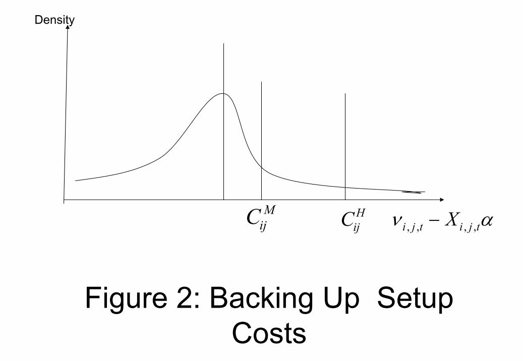
Figure 2: Backing Up Setup Costs
ν αi j t i j tX, , , ,−
Density
CijM Cij
H

Figure 3: The Fraction of Host Countries by the Number of Source Countries Exporting Positive FDI Flows between 1981-98 Max. Number of Source Countries: 12Total Number of Host Countries obs. = 270 (45 * 6)
0
2
4
6
8
10
12
14
16
18
20
22
24
1 2 3 4 5 6 7 8 9 10 11 12
The number of source countries
% o
f tot
al n
umbe
r of h
ost c
ount
ries
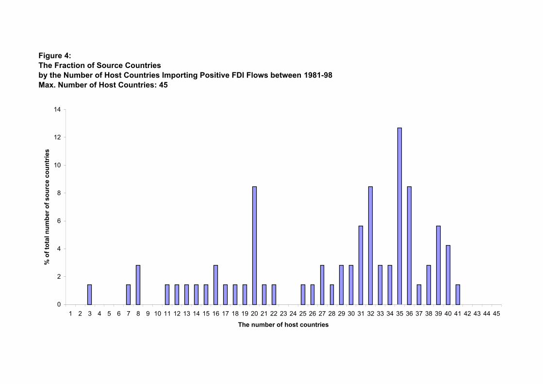
Figure 4: The Fraction of Source Countries by the Number of Host Countries Importing Positive FDI Flows between 1981-98Max. Number of Host Countries: 45
0
2
4
6
8
10
12
14
1 2 3 4 5 6 7 8 9 10 11 12 13 14 15 16 17 18 19 20 21 22 23 24 25 26 27 28 29 30 31 32 33 34 35 36 37 38 39 40 41 42 43 44 45
The number of host countries
% o
f tot
al n
umbe
r of s
ourc
e co
untr
ies
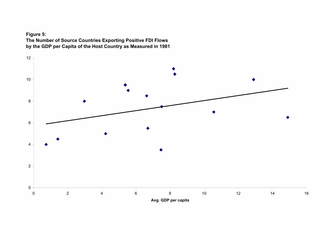
Figure 5: The Number of Source Countries Exporting Positive FDI Flowsby the GDP per Capita of the Host Country as Measured in 1981
0
2
4
6
8
10
12
0 2 4 6 8 10 12 14 16
Avg. GDP per capita

Figure 6: The Number of Source Countries by the Average Years of Schooling in the Host Country*
2
3
4
5
6
7
8
9
10
11
12
2 4 6 8 10 12 14 16 18
Avg. Years of Schooling
* Education is measured by the average number of years of schooling of total population age 25 and older in source (host) country. Source: Barro-Lee
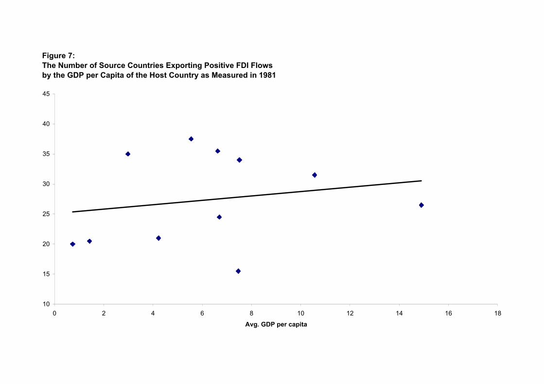
Figure 7: The Number of Source Countries Exporting Positive FDI Flowsby the GDP per Capita of the Host Country as Measured in 1981
10
15
20
25
30
35
40
45
0 2 4 6 8 10 12 14 16 18
Avg. GDP per capita
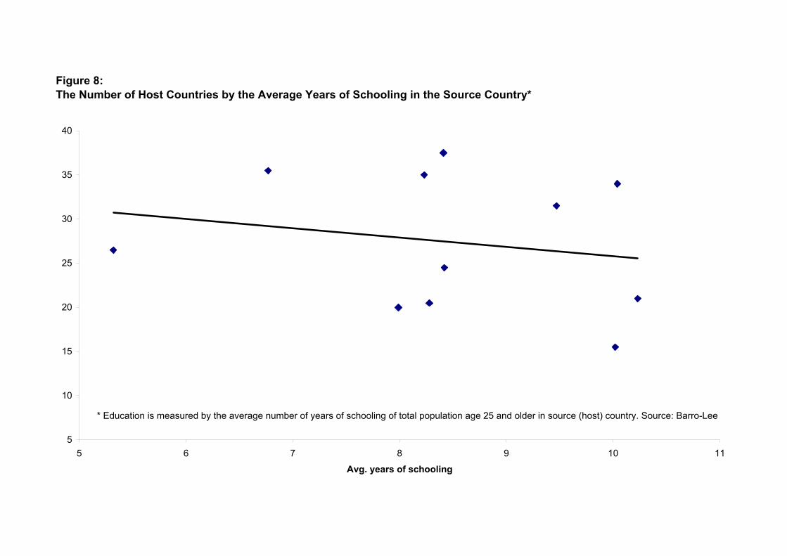
Figure 8: The Number of Host Countries by the Average Years of Schooling in the Source Country*
5
10
15
20
25
30
35
40
5 6 7 8 9 10 11
Avg. years of schooling
* Education is measured by the average number of years of schooling of total population age 25 and older in source (host) country. Source: Barro-Lee

Table 1:The OLS "Gravity" FDI EquationDependent variable: FDI (prices adjusted - in logs)
OLS* OLS*^ OLS* OLS*^ OLS* OLS*^Variables (i) (ii) (iii) (iv) (v) (vi)
GDP of the host country 0.727 0.207(0.031) (0.012)
GDP of the source country 0.926 0.700(0.033) (0.012)
GDP per capita - host 0.904 0.270(0.053) (0.019)
GDP per capita - source 1.656 0.794(0.169) (0.019)
S-H GDP per capita -0.514 0.318(0.053) (0.016)
Average years of schooling - host 0.153 0.045 0.074 0.019(0.018) (0.007) (0.025) (0.009)
Average years of schooling - source 0.154 0.168 0.123 0.128(0.026) (0.007) (0.026) (0.009)
S/H avg. school years ratio -0.002 0.092(0.100) (0.042)
Population - host 0.701 0.199(0.032) (0.012)
Population - source 0.897 0.686(0.034) (0.012)
S-H population gap 0.061 0.250(0.029) (0.010)
Same Language 0.489 0.221 0.564 0.219 0.506 -0.130(0.089) (0.032) (0.091) (0.032) (0.110) (0.039)
Distance -0.005 -0.002 -0.004 -0.002 -0.002 -0.002(0.001) (0.000) (0.001) (0.000) (0.001) (0.000)
Observations 2796 9843 2796 9843 2796 9843
Adj R-square 0.412 0.399 0.419 0.402 0.1074 0.0945
Note:* Replacing missing values (log(0)) with zeros. (Bechmark case)^ Including all possible S-H pairs. (Stage one)All specifications include year fixed-effects.( ) Standard errors in parenthesis
Specification I Specification II Specification III

Table 2:The Complete Gravity Model: FDI Flows and Selection into S-H PairsThe Full Maximum-Likelihood
Variables (i) (ii) (iii)
GDP of the host country^ 0.624(0.036)
GDP of the source country^ 0.567(0.072)
GDP per capita - host^ 0.762(0.054)
GDP per capita - source^ 0.002(0.207)
S-H GDP per capita gap^ -0.091(0.100)
Average years of schooling - host 0.151 0.087(0.016) (0.023)
Average years of schooling - source 0.232 0.295(0.029) (0.025)
S/H avg. school years ratio 0.298(0.112)
Population - host^ 0.583(0.036)
Population - source^ 0.557(0.059)
S-H population gap^ 0.345(0.060)
Same Language 1.249 1.209 0.596(0.082) (0.085) (0.124)
Distance -0.006 -0.006 -0.003(0.001) (0.001) (0.001)
Panel A: Flows Equation: Dependent variable: FDI (prices adjusted - in logs)
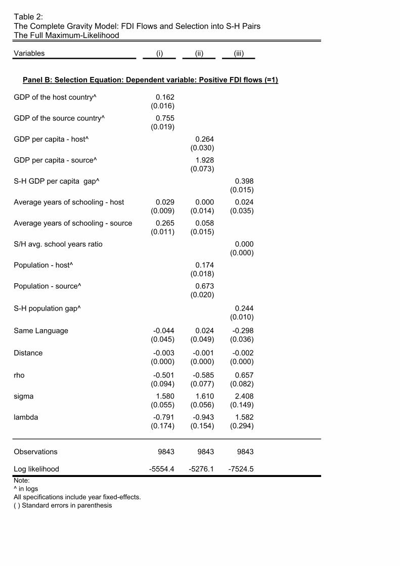
Table 2:The Complete Gravity Model: FDI Flows and Selection into S-H PairsThe Full Maximum-Likelihood
Variables (i) (ii) (iii)
GDP of the host country^ 0.162(0.016)
GDP of the source country^ 0.755(0.019)
GDP per capita - host^ 0.264(0.030)
GDP per capita - source^ 1.928(0.073)
S-H GDP per capita gap^ 0.398(0.015)
Average years of schooling - host 0.029 0.000 0.024(0.009) (0.014) (0.035)
Average years of schooling - source 0.265 0.058(0.011) (0.015)
S/H avg. school years ratio 0.000(0.000)
Population - host^ 0.174(0.018)
Population - source^ 0.673(0.020)
S-H population gap^ 0.244(0.010)
Same Language -0.044 0.024 -0.298(0.045) (0.049) (0.036)
Distance -0.003 -0.001 -0.002(0.000) (0.000) (0.000)
rho -0.501 -0.585 0.657(0.094) (0.077) (0.082)
sigma 1.580 1.610 2.408(0.055) (0.056) (0.149)
lambda -0.791 -0.943 1.582(0.174) (0.154) (0.294)
Observations 9843 9843 9843
Log likelihood -5554.4 -5276.1 -7524.5Note:^ in logsAll specifications include year fixed-effects.( ) Standard errors in parenthesis
Panel B: Selection Equation: Dependent variable: Positive FDI flows (=1)

Table 3:The OLS "Gravity" FDI Equation - OECD Countries OnlyDependent variable: FDI (prices adjusted - in logs)
OLS* OLS*^ OLS* OLS*^Variables (i) (ii) (iii) (iv)
GDP of the host country 0.712 0.192(0.184) (0.070)
GDP of the source country 0.930 0.922(0.175) (0.080)
GDP per capita - host -1.782 -0.740(0.701) (0.280)
GDP per capita - source 1.868 1.123(0.723) (0.105)
Average years of schooling - host 0.193 0.041 0.282 0.066(0.136) (0.051) (0.151) (0.054)
Average years of schooling - source 0.061 0.240 0.065 0.163(0.140) (0.030) (0.150) (0.045)
Population - host 0.789 0.221(0.181) (0.070)
Population - source 0.928 0.896(0.175) (0.078)
Same Language -0.368 -0.030 -0.490 -0.131(0.627) (0.229) (0.623) (0.233)
Distance -0.002 -0.002 -0.003 -0.001(0.003) (0.001) (0.003) (0.001)
Observations 795 2796 795 2796
Adj R-square 0.254 0.429 0.297 0.444
Note:* Replacing missing values (log(0)) with zeros. (Bechmark case)^ Including all possible S-H pairs. (Stage one)All specifications include year fixed-effects.( ) Standard errors in parenthesis
Specification I Specification II

Table 4:The Complete Gravity Model: FDI Flows and Selection into S-H Pairs Sample: OECD Countries OnlyThe Full Maximum-Likelihood
Variables (i) (ii)
GDP of the host country^ 0.669(0.113)
GDP of the source country^ 0.366(0.151)
GDP per capita - host^ -1.251(0.502)
GDP per capita - source^ 0.143(0.682)
Average years of schooling - host 0.285 0.394(0.069) (0.080)
Average years of schooling - source 0.156 0.346(0.078) (0.080)
Population - host^ 0.797(0.111)
Population - source^ 0.629(0.164)
Same Language 1.686 1.408(0.344) (0.375)
Distance -0.007 -0.010(0.002) (0.002)
Panel A: Flows Equation: Dependent variable: FDI (prices adjusted - in logs)

Table 4:The Complete Gravity Model: FDI Flows and Selection into S-H Pairs Sample: OECD Countries OnlyThe Full Maximum-Likelihood
Variables (i) (ii)
GDP of the host country^ 0.072(0.072)
GDP of the source country^ 0.790(0.102)
GDP per capita - host^ -0.632(0.343)
GDP per capita - source^ 2.363(0.272)
Average years of schooling - host 0.003 -0.017(0.052) (0.063)
Average years of schooling - source 0.291 0.039(0.040) (0.066)
Population - host^ 0.060(0.089)
Population - source^ 0.775(0.122)
Same Language -0.421 -0.377(0.222) (0.256)
Distance -0.002 0.001(0.001) (0.001)
rho -0.783 -0.661(0.109) (0.219)
sigma 1.775 1.537(0.171) (0.159)
lambda -1.389 -1.015(0.306) (0.430)
Observations 2796 2796
Log likelihood -1812 -1654Note:^ in logsAll specifications include year fixed-effects.( ) Standard errors in parenthesis
Panel B: Selection Equation: Dependent variable: Positive FDI flows (=1)