Which CL are you really flying ? &

Some ideas about aerodynamic optimization

matthieu.scherrer@free.fr March 2007

For the scientific modeller, many tools are available on the Internet for optimizing sailplane aerodynamics. Xfoils give access to very refined airfoils characteristics, whereas program as Nurflugel or AVL gives an insight into finite wing design. Finally tools like MIAReX or XFLR5 merges both view, i.e. Xfoil and finite wing. So, this is very cool, you can compute CL, CD for wings over large variation of many parameters (α, Re number, platform, etc…). The task might be simply expressed for aerodynamic geek :

“L/D augment you shall” Nevertheless, when performing optimization, we do observe aerodynamicist life is not that easy. It is not possible to enhance any part of the glider polar, but there are often trade off to accept.

What would be great to do… …and what

0

0.2

0.4

0.6

0.8

1

1.2

1.4

1.6

0 0.005

CL

0

0.2

0.4

0.6

0.8

1

1.2

1.4

1.6

0 0.005 0.01 0.015 0.02CD

CL

More lift, less drag

Then comes the question :

What is best to optimize, and where should we p This study is trying to answer this question, through a statistical studexperience during flights.

Recording a flight The first step is to be able to evaluate CL during flight. This is not nLift coefficient is given by :

SmgV

VVNzCCAS

L0

12

21 2 with ,

ρ==

With NZ the acceleration normal to the glider, V1 the speed of the gcondition (function of wing loading m/S) and VCAS is airspeed (calThis is all you need to know during the flight to compute CL.

less drag at some point,but less lift too

is possible to do.

0.01 0.015 0.02CD

ut our efforts ?

y of what our sailplane do

ecessarily an easy task.

lider for CL=1 in standard ibrated airspeed).

First I tried using portable GPS in recording mode within “big sailplane”. It was difficult to trust the values obtained, as :

• The rate of measurement is low (1 record per second max). • You have to evaluate the acceleration Nz from path, which is not that accurate. • You have to evaluate wind at any altitude, since GPS speed is ground speed.

To put it in a nutshell, you have to extract much information from scarce recording. This ends in a quite large uncertainty about CL values.

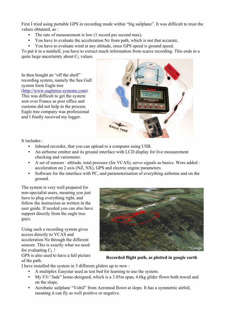
In then bought an “off the shelf” recording system, namely the Sea Gull system form Eagle tree (http://www.eagletree-systems.com). This was difficult to get the system sent over France as post office and customs did not help in the process. Eagle tree company was professional and I finally received my logger.

It includes :

• Inboard recorder, that you can upload to a computer using USB. • An airborne emitter and its ground interface with LCD display for live measurement

checking and variometer. • A set of sensors : altitude, total pressure (for VCAS), servo signals as basics. Were added :

acceleration on 2 axis (NZ, NX), GPS and electric engine parameters. • Software for the interface with PC, and parameterisation of everything airborne and on the

ground. The system is very well prepared for non-specialist users, meaning you just have to plug everything right, and follow the instruction as written in the user guide. If needed you can also have support directly from the eagle tree guys. Using such a recording system gives access directly to VCAS and acceleration Nz through the different sensors. This is exactly what we need for evaluating CL ! GPS is also used to have a full picture of the path.

Recorded flight path, as plotted in google earth

I have installed the system in 3 different gliders up to now : • A multiplex Easystar used as test bed for learning to use the system. • My F3i “Jade” home-designed, which is a 3.85m span, 4.6kg glider flown both towed and

on the slope. • Aerobatic sailplane “VoltiJ” from Aeromod flown at slope. It has a symmetric airfoil,

meaning it can fly as well positive or negative.

Easytar electric sailplane

Voltij aerobatic sailplane Jade F3i competition sailplane

GPS antennaPitot tube

Eagletree recorder Data transmitter antenna

Quick-and-dirty installation on board of Easystar test bed

Some preparation is necessary to have quality measurement. • You need to installed a Pitot tube for measuring airspeed VCAS. Recommendations are

given in the Eagletree user guide. Theoretically, measurement is sensible the location of both Pitot tube and static probe. I have investigated the accuracy of airspeed by comparing with GPS speed. I was able to repeatedly evaluate a 5kph wind in altitude, meaning the accuracy should be higher than 2.5kph.

• Acceleration sensor is to be calibrated, and need to be installed as close as possible as CG location (the wire for this sensor is somewhat short with respect to that).

Once everything is installed on board, using the system everyday is easy. When you power the sailplane, the init of the system begins. The dashboard is very useful for checking “live” that everything is running correctly. GPS coverage can be displayed, and all you need is wait for some 1-2minutes before enough GPS satellites are contacted. This being made, you just have to fly the glider. The recording duration depends on the recording rate. I use 2 record per second giving approx. one hour of recording with the full set of sensor. This duration can vary with the activity of the flight.

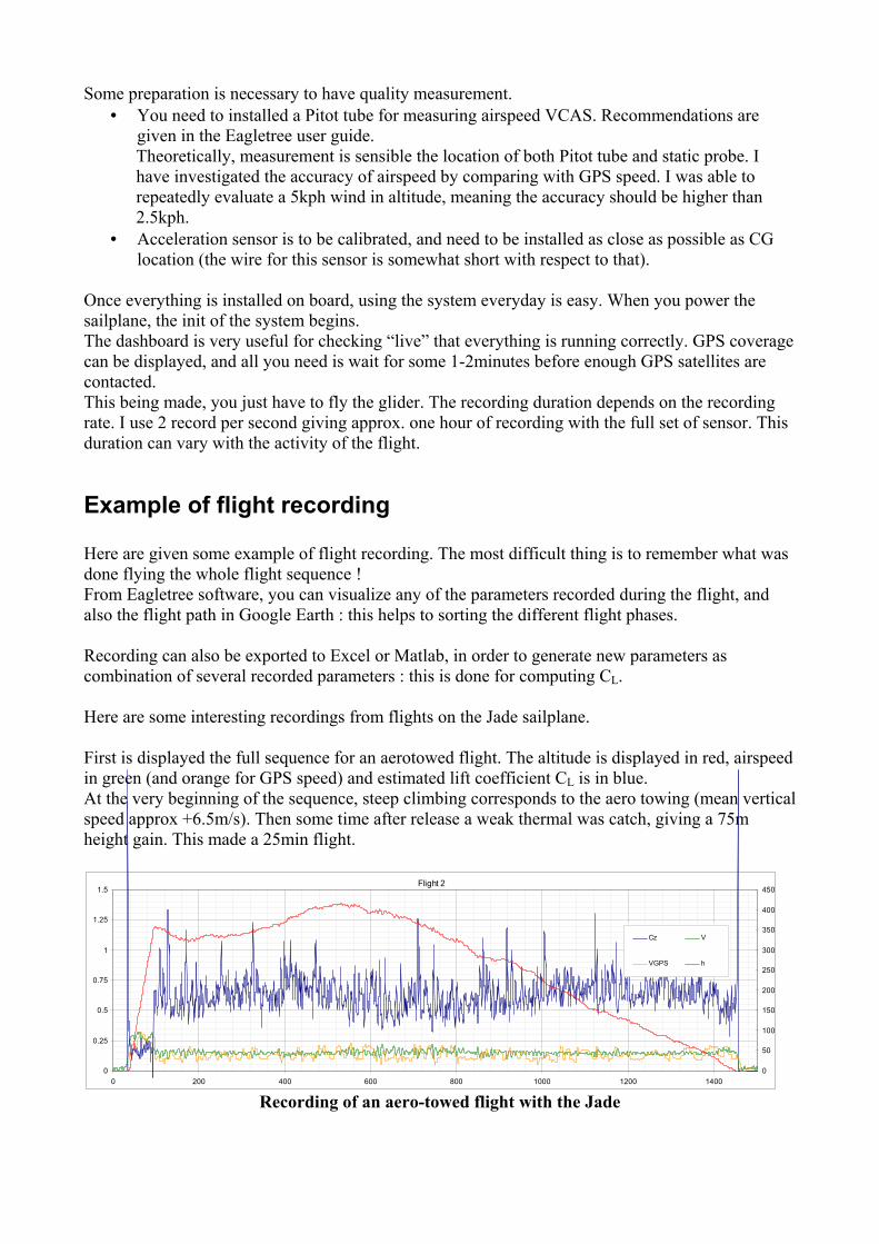
Example of flight recording Here are given some example of flight recording. The most difficult thing is to remember what was done flying the whole flight sequence ! From Eagletree software, you can visualize any of the parameters recorded during the flight, and also the flight path in Google Earth : this helps to sorting the different flight phases. Recording can also be exported to Excel or Matlab, in order to generate new parameters as combination of several recorded parameters : this is done for computing CL. Here are some interesting recordings from flights on the Jade sailplane. First is displayed the full sequence for an aerotowed flight. The altitude is displayed in red, airspeed in green (and orange for GPS speed) and estimated lift coefficient CL is in blue. At the very beginning of the sequence, steep climbing corresponds to the aero towing (mean vertical speed approx +6.5m/s). Then some time after release a weak thermal was catch, giving a 75m height gain. This made a 25min flight.

Flight 2

0

0.25

0.5

0.75

1

1.25

1.5

0 200 400 600 800 1000 1200 14000

50

100

150

200

250

300

350

400

450

Cz V

VGPS h

Recording of an aero-towed flight with the Jade

Next cession is the recording a simple looping manoeuvre during another aero towed flight. This gives an idea of the condition encountered by the sailplane in such a manoeuvre. The entry speed was roughly 155 kph and a gentle pull up (CL≈0.3) created 5.5Gs (black curve on the lower part of the graphic). The diameter was approx 45m. At the end of the manoeuvre, the speed was around 135kph, and altitude was 20m lower than in the beginning.

Paramètres de vol

0

0.25

0.5

0.75

1

1.25

1.5

255 260 265 270 275 2800

50

100

150

200

250

300

CLV (kph)h (m)

Looping

Paramètres de vol

-1

0

1

2

3

4

5

6

7

255 260 265 270 275 280

Battery (V)Nz (G)

Looping

Recording of a looping of Jade

Last but not least, here is a DS sequence flown on a calm day (15kph wind). This gives some information about aerodynamic parameters while DSing. The flight did look very gentle, as needed for a big lady as Jade sailplane. Already the condition encountered in such calm DS cession may seem tough! Some facts :

• From the altitude variation the mean radius of the path was around 45m (path considered as a 45deg tilted circle), and airspeed oscillate about +/-20kph around a mean value of 120kph.

• On each lap, the acceleration reaches round 6Gs, with some peak around 7gs. • The airspeed increase when, crossing the shear layer can be observed twice per lap, as “in

the book” : in the down leg and in the up leg. • Negative G’s, hence negative values for CL are encountered while crossing the shear layer.

Paramètres de vol

-0.4

-0.2

0

0.2

0.4

0.6

0.8

1

1200 1225 1250 1275 1300 1325 1350

0

20

40

60

80

100

120

140

CL

V (kph)

h (m)

Paramètres de vol

-4

-2

0

2

4

6

8

1200 1225 1250 1275 1300 1325 1350

Battery (V)

Nz (G)

Recording of 13 laps while DSing the Jade

This sequence closes the first part about raw experimental material.

Statistical study of a flight : the “flight template” There is a lot of information to treat within flight recording. In order to be focused on the most important results, a post-treatment of time CL history was performed. The objective is to have a statistical representation of the flight :

Following plots are giving an image of how many time was spent for each value of CL during the flight.

I have called this a "flight template", which represents the relative density of each CL. Here is given a typical example of flight template :

Typical flight template

-0,25 0 0,25 0,5 0,75 1 1,25

CL

dt/d

CL

3

21

Horizontal axis represents value of lift coefficient CL. On the vertical axis, the higher the value for one CL, the longer time was spent for this CL. Note that vertical axis values have no direct physical meaning. From former figure, several points can be addressed :

• The minimum value of lift coefficient reached during this flight is approx CL = -0.1 (1) • The maximum lift coefficient value reached is approx CL = 1.1 (2) • Most of the time during this flight was spent flying the lift coefficient around the main peak

of the curve, meaning between CL≈0.30 & CL ≈0.55 (3) Such a curve can be used for summarizing the flight at first sight, for it gives a qualitative and quantitative content of the flight you have performed. Note that such a curve can "a priori" be different for each flight, dependant upon several parameters, such as wing loading, etc... But surprisingly, general rules do appear independently from the kind of sailplane flown.

This means some aerodynamic paramount does exist for models, leading to design rules.

But lets talk first about practical examples of the so called “flight template”.

Practical example of flight template

Easystar I have been flying the Easystar electric glider quite extensively with eagle tree system onboard, without specific objective in flight : to put it in a nutshell, just flying for fun. I have picked up 7 flights and generated corresponding “flight templates”, representing approx 3hours of typical flight for this model : climbing in thermal when possible, playing at low altitude, etc… At the end we have here a summary of a typical flight condition for “everyday flight” on small sailplane.

Flight template

-0.25 0 0.25 0.5 0.75 1 1.25

CL

dt/d

CL

Zizi 27sept06Zizi 2oct06Zizi 8oct06-2Zizi 14oct0629 oct 06Zizi 16dec06Zizi 06jan07

Flight template obtained flying the Easystar

Several conclusions can be drawn from those curves:

• Evidence are converging to the fact that most of the time is spent flying in the 0.5-.075 CL range. This remains true over a wide range of “flight style”.

• The upper limit of CL experienced flying the Easystar is around CL. The airfoil being able to generate such a lift, it is used, but not that often.

• The more active flight, the lower the main peak and the wider its basis (“flatter” curve).

Jade sailplane Here are now described flight templates for 7 flights performed over 3 flight cessions. This summarizes close to 2h30 of effective flight time in different condition.

Flight template

-0,25 0 0,25 0,5 0,75 1 1,25

CL

dt/d

CL

Jade slope Flight 1Jade slope Flight 2Jade aerotowed Flight 1Jade aerotowed Flight 2Jade aerotowed Flight 3Jade aerotowed Flight 4Jade aerotowed Flight 5

1

2

5 4

1 2

3

Flight template obtained flying the Jade

In blue, two flights perform at slope, in altitude (1700m, Port de Bales in French Pyrenees mountains). In red three flights performed over flat land with aero towed start, on a fair day with broad but weak thermals. In orange flights from the same place, on a calm day with so to speak no lift. Several conclusion can be drawn for those data :

• At slope with very windy condition (blue line nb1) the need for lift coefficient is very reduced (CL=0.5 maximum). Most of the time is spent flying CL within 0.07-0.25 range. NB : this is probably a good indication of the fact that the wing loading was too low for this windy day…

• At slope with good condition but with less wind (blue line nb2), it can be observed that most of the time is speed flying CL around 0.15 - 0.5 which is quite low again. But this time, maximum value reached is around CL=0.9 - 1.

• Over flat land with low wind condition (red and orange curve), it seems most of the time is spent around CL=0.6, whatever the condition. This is in line with result from Easystar, even if the design is really different.

• Slightly negative values for CL are encountered, even without performing aerobatics. • The longer the flight while seeking thermal (red curves, weak thermal available), the more

flight template is focused around the mean value the typical CL. And the lower the curves at the extremity of the CL range.

• The shorter the flight and/or the more “activity” in the flight (orange curves, no thermal available : short flights and aerobatics), the flatter and wider flight template is, as the whole flight domain is more equally flown.

Voltij sailplane Here are flight templates for 2 flight performed at slope in fair lift condition. This represents approx. 0h40 of effective flight time while performing various aerobatics manoeuvres. This were quite “active flights”

Flight template

-1.25 -1 -0.75 -0.5 -0.25 0 0.25 0.5 0.75 1 1.25

CL

dt/d

CL

Voltij - Flight 1

Voltij - Flight 2

Flight template obtained flying the Voltij

Several conclusion can be drawn for those data :

• The positive CL part is quite consistent with results obtained from Jade sailplane flown at slope.

• Once again the need for high CL is not often verified. Nevertheless in the detail, it seems more (negative) lift is used in inverted flight than in positive.

• A symmetrical sailplane as Voltij can be use symmetrically, as mean peaks for positive and negative CL are symmetrically shared.

• The relative heights of the peaks for positive & negative CL means how many time was spent in normal flight / in inverted flight (here roughly 2/3 in positive, 1/3 in negative)

Airfoil analysis and design rules using lessons learned from flight templates Use of flight template in airfoil & sailplane design A flight template gives basically the image of which part of the CL is flown the more often. Then it comes quite logically to the mind following statement :

We should optimize the aerodynamic characteristics for the CL conditions that are the most flown.

To put it in a nutshell, the higher the flight template for one CL condition, the higher attention should be paid at the aerodynamic characteristic, and the more effort should be dedicated to reducing drag for this CL. The two typical flight template defined for slope flight and flight over flat land can now be used for helping designing of all around sailplane. For competition tasks, new specific flight template must be defined for helping designing for corresponding competitions.

Based on a given flight template, two main strategy for optimising aerodynamic characteristics can be adopted :

Typical flight template

-0,25 0 0,25 0,5 0,75 1 1,25

CL

dt/d

CL

• Maximise performance within the most flown area at any cost elsewhere This means optimizing only the most flown part of the domain (bold lines on chart) according to the “flight programme” depicted by the flight template. This is a risky strategy, as high CL are not flown very often, but nevertheless might be needed over a short period of time. This can be considered for hot competition sailplane, designing the best for the task represented by the flight template, but probably exhibiting a narrow flight domain, restricted to the completion of the task. • Maximise drag performance with attention paid to highest lift coefficients This means optimizing the most flown part of the domain (bold lines on chart) but also considering reaching the limit of the flown domain (doted lines). This is a less risky strategy, as some efforts are dedicated to fulfilling the upper end of the CL range. The sailplane will for sure be less slippery, as it will accept higher lift situation. Nevertheless it is not possible anymore to optimize as much the “peaky CL” range of the flight template.

NB : optimizing according to flight template is related to minimizing energy absorbed by drag. Strategy for automated numerical optimization can be derived, for more information see : http://perso.orange.fr/scherrer/matthieu/aero/papers/Flight%20template_OSTIV.pdf http://perso.orange.fr/scherrer/matthieu/aero/papers/Ostiv%20presentation%20V2.ppt

Typical “everyday flights” We have compiled all the data obtained through flight-testing on different sailplane in different conditions. Common conditions that can be encountered when flying model of sailplanes have been covered. It is now possible to define two “statistical flight templates”, representing two main CL range of conditions for flights either at slope or over flat land, whatever the sailplane : Typical flight performed at slope (in dark blue) :

• The airfoil is the most often used around CL=0.3 • Typical CL range of most use is 0.15 to 0.6 • Nevertheless, CL over 1 are flown, but not over a long period of time

NB : conclusion drawn here would be different when considering a F3F run, as the flight is much shorter and proportion of tight turn much higher. Typical flight performed over flat land (in red) :

• The airfoil is the most often used around CL=0.6 • Typical CL range most use is 0.3 to 0.8 • Nevertheless, CL up to 1.1 - 1.2 are flown, but not over a long periods of time

NB : conclusion drawn here might probably stand for duration tasks in competitions.

Flight template

-0.25 0 0.25 0.5 0.75 1 1.25

CL

dt/d

CL

Typical flightat slope

Typical flight over flat land

Typical flight template to consider for “everyday flights”

Illustrated use of flight template for airfoil selection Let’s have a look at the following test case. Hereafter are displayed Xfoil polars for the MG06 (very successful in 60inch class) and RG15, at rather low Re condition. According to those results :

• If we consider typical flight over flat land, we see that in the most often flown CL range (red, bold line on the left) RG15 do exhibit lower drag than MG06.

• For typical slope condition, this time MG06 has a lower drag than RG15 in the most often flown CL range (blue, bold line on the left).

At the end, RG15 seems a better all around airfoil than MG06, whereas MG06 is better adapted than RG15 to slope flying. Additionally the fact that MG06 is able to generate high lift at low Re numbers should make sailplane equipped with it easy to fly. This fits rather well with the observation in flight for 60inches glider equipped with those airfoils. NB : for completing the full view effect of flaps should be studied, as the MG06 range of use do improve much with dynamic use of flap.

Airfoil polars & range of use as described by flight template

Conclusion I hope you now have a better idea of the aerodynamic conditions as encountered by our sailplane models, and accordingly what needs to be done for better-optimized gliders. This was at first not an easy task to define a process that allows proper estimates of lift coefficients we are actually flying, as we are not in the sailplane.

Based on recordings, I have built the concept of “flight templates”, that are curves describing the content of the flight in term of lift coefficient CL. For “everyday flying”, typical template for flying at slope and over flat land have been extracted. It has been shown that some parts of the CL range are most often used than other. Surprisingly, value the most often flown lift coefficients, around CL≈0.5-0.6, may seem rather low. Nevertheless higher CL are experienced, over shorter period of time. For competition task flight template can be as well derived, for defining very precise aerodynamic specification for the optimization process. With the knowing of those statistical studies of flights, new optimization strategies can now be adopted, in order to design sailplanes that fit with the use we make of them. I now wish you happy designing and flying with the benefit of all this information !!