Where Quants Go Wrong - Institutional Money · 2009-03-05 · Where Quants Go Wrong A dozen basic...
83
Where Quants Go Wrong A dozen basic lessons in commonsense for quants and risk managers and the traders who rely on them Paul Wilmott Paul Wilmott is a financial consultant, specializing in derivatives, risk management and quan- titative finance. Paul is the author of Paul Wilmott Introduces Quantitative Finance (Wiley 2007), Paul Wilmott On Quantitative Finance (Wiley 2006), Frequently Asked Questions in Quantitative Finance (Wiley 2006) and other financial textbooks. He has written over 100 research articles on finance and mathematics. Paul Wilmott was a founding partner of the volatility arbitrage hedge fund Caissa Capital which managed $170million. His responsibilities included forecasting, derivatives pricing, and risk management. Dr Wilmott is the proprietor of www.wilmott.com, the popular quantitative finance commu- nity website, the quant magazine Wilmott and is the Course Director for the Certificate in Quantitative Finance www.7city.com/cqf. The CQF teaches how to apply mathematics to finance, focusing on implementation and pragmatism, robustness and transparency. c Paul Wilmott 1
Transcript of Where Quants Go Wrong - Institutional Money · 2009-03-05 · Where Quants Go Wrong A dozen basic...
Where Quants Go WrongA dozen basic lessons in commonsense forquants and risk managers and the traders
who rely on them
Paul Wilmott
Paul Wilmott is a financial consultant, specializing in derivatives, risk management and quan-titative finance. Paul is the author of Paul Wilmott Introduces Quantitative Finance (Wiley2007), Paul Wilmott On Quantitative Finance (Wiley 2006), Frequently Asked Questions inQuantitative Finance (Wiley 2006) and other financial textbooks. He has written over 100research articles on finance and mathematics.
Paul Wilmott was a founding partner of the volatility arbitrage hedge fund Caissa Capitalwhich managed $170million. His responsibilities included forecasting, derivatives pricing, andrisk management.
Dr Wilmott is the proprietor of www.wilmott.com, the popular quantitative finance commu-nity website, the quant magazine Wilmott and is the Course Director for the Certificate inQuantitative Finance www.7city.com/cqf. The CQF teaches how to apply mathematics tofinance, focusing on implementation and pragmatism, robustness and transparency.
c©Paul Wilmott
1

Quants and risk managers keep making the same mistakes over
and over again. Each time this happens the losses increase in
value. A small amount of commonsense and some basic mathe-
matics can stop this happening. However, this requires quants,
risk managers and their bosses to move their attention away from
complexity towards robustness of models.∗
Keywords: Jensen’s inequality; Sensitivity to parameters; Corre-
lation; Diversification; Dynamic hedging; Feedback; Supply and
demand; Closed-form solutions; Calibration; Modelling; Preci-
sion; Nonlinearity; CSI Miami
c©Paul Wilmott
∗This paper was borne out of a CQF lecture (www.7city.com/cqf) and aseries of blogs (www.wilmott.com/blogs/paul).
2
Topics
• Lack of diversification
• Supply and demand
• Jensen’s inequality arbitrage
• Sensitivity to parameters
• Correlation
• Reliance on continuous hedging (arguments)
• Feedback
• Reliance on closed-form solutions
• Valuation is not linear
• Calibration
• Too much precision
• Too much complexity
c©Paul Wilmott
3

But first a simple test-yourself quiz.
c©Paul Wilmott
4
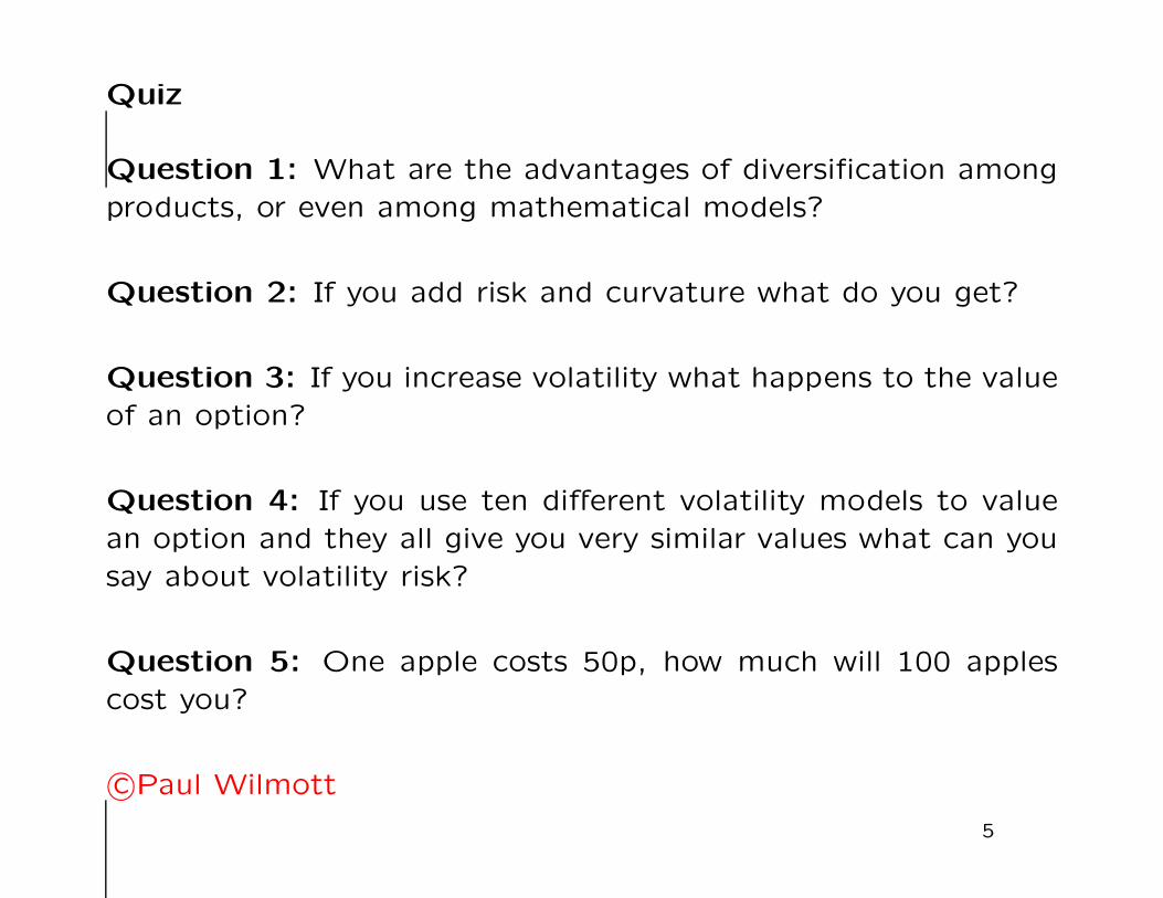
Quiz
Question 1: What are the advantages of diversification amongproducts, or even among mathematical models?
Question 2: If you add risk and curvature what do you get?
Question 3: If you increase volatility what happens to the valueof an option?
Question 4: If you use ten different volatility models to valuean option and they all give you very similar values what can yousay about volatility risk?
Question 5: One apple costs 50p, how much will 100 applescost you?
c©Paul Wilmott
5
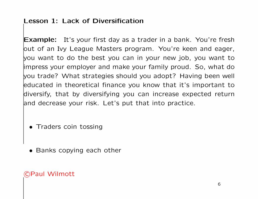
Lesson 1: Lack of Diversification
Example: It’s your first day as a trader in a bank. You’re fresh
out of an Ivy League Masters program. You’re keen and eager,
you want to do the best you can in your new job, you want to
impress your employer and make your family proud. So, what do
you trade? What strategies should you adopt? Having been well
educated in theoretical finance you know that it’s important to
diversify, that by diversifying you can increase expected return
and decrease your risk. Let’s put that into practice.
• Traders coin tossing
• Banks copying each other
c©Paul Wilmott
6

Keynes said, “It is better to fail conventionally than to succeed
unconventionally.”
There is no incentive to diversify while you are playing with OPM
(Other People’s Money).
Example: Exactly the same as above but replace ‘trades’ with
‘models.’ There is also no incentive to use different models from
everyone else, even if your are better.
c©Paul Wilmott
7

There’s a timescale issue here as well. Anyone can sell deep
OTM puts for far less than any ‘theoretical’ value, not hedge
them, and make a fortune for a bank, which then turns into a
big bonus for the individual trader. You just need to be able to
justify this using some convincing model. Eventually things will
go pear shaped and you’ll blow up. However, in the meantime ev-
eryone jumps onto the same (temporarily) profitable bandwagon,
and everyone is getting a tidy bonus. The moving away from un-
profitable trades and models seems to be happening slower than
the speed at which people are accumulating bonuses from said
trades and models!
c©Paul Wilmott
8

Envy:
We all know of behavioural finance experiments such as the fol-
lowing two questions.
First question, people are asked to choose which world they
would like to be in, all other things being equal, World A or
World B where
A. You have 2 weeks’ vacation, everyone else has 1 week
B. You have 4 weeks’ vacation, everyone else has 8 weeks
The large majority of people choose to inhabit World B. They
prefer more holiday to less in an absolute sense, they do not
suffer from vacation envy.
c©Paul Wilmott
9
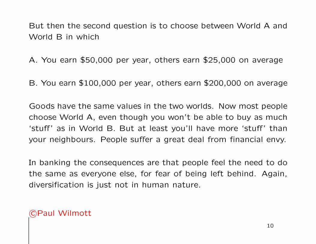
But then the second question is to choose between World A and
World B in which
A. You earn $50,000 per year, others earn $25,000 on average
B. You earn $100,000 per year, others earn $200,000 on average
Goods have the same values in the two worlds. Now most people
choose World A, even though you won’t be able to buy as much
‘stuff’ as in World B. But at least you’ll have more ‘stuff’ than
your neighbours. People suffer a great deal from financial envy.
In banking the consequences are that people feel the need to do
the same as everyone else, for fear of being left behind. Again,
diversification is just not in human nature.
c©Paul Wilmott
10

Lesson 2: Supply and Demand
Supply and demand is what ultimately drives everything! Butwhere is the supply and demand parameter or variable in Black–Scholes?
A trivial observation: The world is net long equities after youadd up all positions and options. So, net, people worry aboutfalling markets. Therefore people will happily pay a premiumfor out-of-the-money puts for downside protection. The resultis that put prices rise and you get a negative skew. That skewcontains information about demand and supply and not aboutthe only ‘free’ parameter in Black–Scholes, the volatility.
The complete-market assumption is obviously unrealistic, andimportantly it leads to models in which a small number of pa-rameters are used to capture a large number of effects.
c©Paul Wilmott
11

The price of milk is a scalar quantity that has to capture in a sin-gle number all the behind-the-scenes effects of, yes, production,but also supply and demand, salesmanship, etc. Perhaps thepint of milk is even a ‘loss leader.’ A vector of inputs producesa scalar price.
So, no, you cannot back out the cost of production from a singleprice.
Similarly
• you cannot back out a precise volatility from the price ofan option when that price is also governed by supply anddemand, fear and greed, not to mention all the imperfectionsthat mess up your nice model (hedging errors, transactioncosts, feedback effects, etc.).
c©Paul Wilmott
12
Supply and demand dictate prices, assumptions and models im-
pose constraints on the relative prices among instruments. Those
constraints can be strong or weak depending on the strength or
weakness of the assumptions and models.
c©Paul Wilmott
13

Lesson 3: Jensen’s Inequality Arbitrage
Jensen’s Inequality states that if f(·) is a convex function and x
is a random variable then
E [f(x)] ≥ f (E[x]) .
This justifies why non-linear instruments, options, have inherent
value.
c©Paul Wilmott
14

Example: You roll a die, square the number of spots you get,
and you win that many dollars. How much is this game worth?
(Assuming you expect to break even.) We know that the average
number of spots on a fair die is 312 but the fair ‘price’ for this
bet is not(312
)2.
For this exercise f(x) is x2, it is a convex function. So
E[x] = 312
and
f (E[x]) =(312
)2= 121
4.
But
E [f(x)] =1 + 4 + 9 + 16 + 25 + 36
6= 151
6 > f (E[x]) .
The fair price is 1516.
c©Paul Wilmott
15
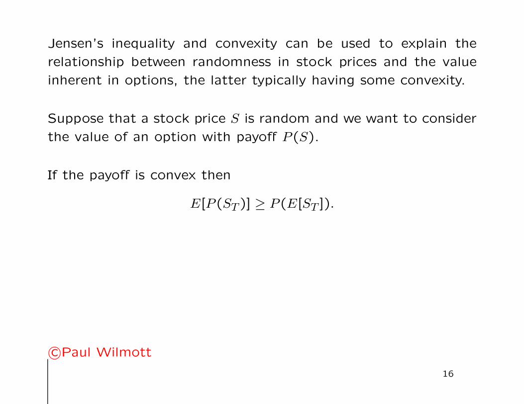
Jensen’s inequality and convexity can be used to explain the
relationship between randomness in stock prices and the value
inherent in options, the latter typically having some convexity.
Suppose that a stock price S is random and we want to consider
the value of an option with payoff P(S).
If the payoff is convex then
E[P(ST )] ≥ P(E[ST ]).
c©Paul Wilmott
16

We can get an idea of how much greater the left-hand side is
than the right-hand side by using a Taylor series approximation
around the mean of S. Write
S = S + ε,
where S = E[S], so E[ε] = 0. Then
E [f(S)] = E[f(S + ε)
]= E
[f(S) + εf ′(S) + 1
2ε2f ′′(S) + · · ·]
≈ f(S) + 12f ′′(S)E
[ε2
]
= f(E[S]) + 12f ′′(E[S])E
[ε2
].
Therefore the left-hand side is greater than the right by approx-
imately
12f ′′(E[S]) E
[ε2
].
c©Paul Wilmott
17

This shows the importance of two concepts
• f ′′(E[S]): This is the convexity of an option. As a rule this
adds value to an option. It also means that any intuition we
may get from linear contracts (forwards and futures) might
not be helpful with non-linear instruments such as options.
• E[ε2
]: This is the variance of the return on the random un-
derlying. Modelling randomness is the key to valuing options.
The lesson to learn from this is that whenever a contract has
convexity in a variable or parameter, and that variable or pa-
rameter is random, then allowance must be made for this in the
pricing.
c©Paul Wilmott
18
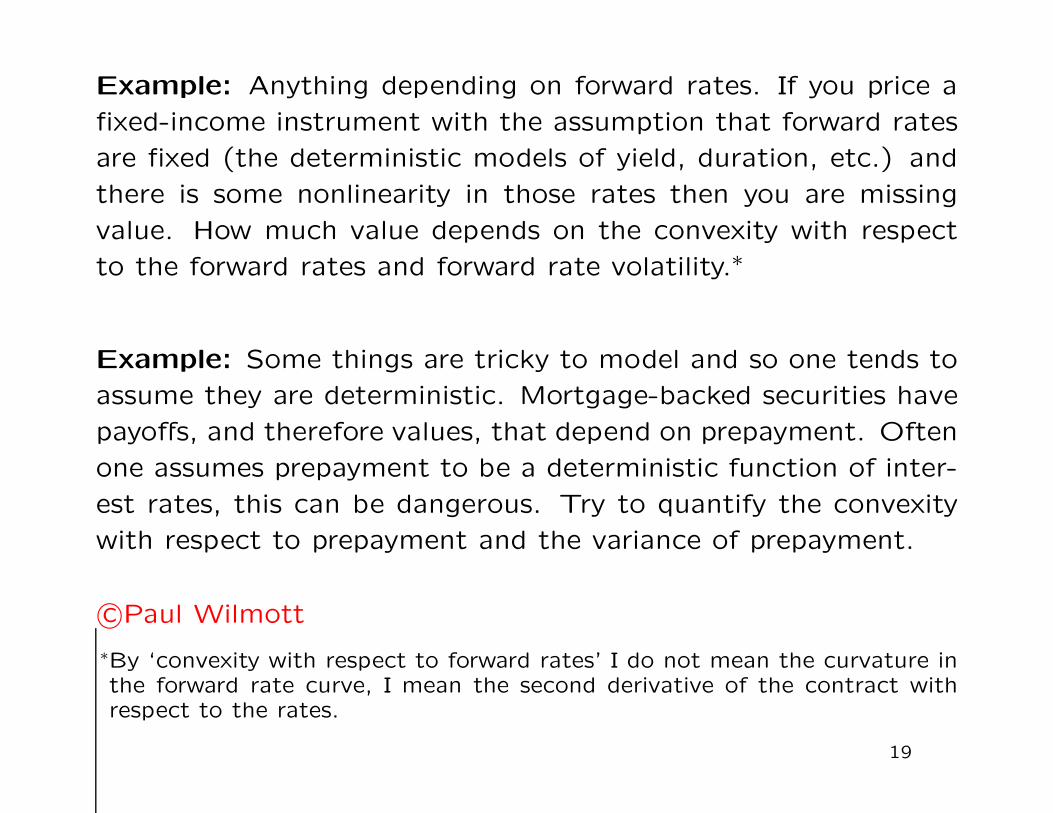
Example: Anything depending on forward rates. If you price a
fixed-income instrument with the assumption that forward rates
are fixed (the deterministic models of yield, duration, etc.) and
there is some nonlinearity in those rates then you are missing
value. How much value depends on the convexity with respect
to the forward rates and forward rate volatility.∗
Example: Some things are tricky to model and so one tends to
assume they are deterministic. Mortgage-backed securities have
payoffs, and therefore values, that depend on prepayment. Often
one assumes prepayment to be a deterministic function of inter-
est rates, this can be dangerous. Try to quantify the convexity
with respect to prepayment and the variance of prepayment.
c©Paul Wilmott
∗By ‘convexity with respect to forward rates’ I do not mean the curvature inthe forward rate curve, I mean the second derivative of the contract withrespect to the rates.
19

Lesson 4: Sensitivity To Parameters
If volatility goes up what happens to the value of an option?Did you say the value goes up? Oh dear, bottom of the class foryou! I didn’t ask what happens to the value of a vanilla option,I just said “an” option, of unspecified terms.
• Pricing an up-and-out call option
• Early-morning panic
• Vega
• Getting fired
c©Paul Wilmott
20

What went wrong was that you assumed volatility to be con-
stant in the option formula/model and then you changed that
constant. This is only valid if you know that the parameter is
constant but are not sure what that constant is. But that’s not
a realistic scenario in finance. In fact, I can only think of one
scenario where this makes sense. . .
• A hot tip from God
c©Paul Wilmott
21

By varying a constant parameter you are effectively measuring
∂V
∂ parameter.
This is what you are doing when you measure the ‘greek’ vega:
vega =∂V
∂σ.
But this greek is misleading. Those greeks which measure sen-
sitivity to a ‘variable’ are fine, those which supposedly measure
sensitivity to a ‘parameter’ are not. Plugging different constants
for volatility over the range 17% to 23% is not the same as exam-
ining the sensitivity to volatility when it is allowed to roam freely
between 17 and 23% without the constraint of being constant.
I call such greeks “bastard greeks” because they are illegitimate.
c©Paul Wilmott
22

An example:
Barrier value, various vol scenarios
0.0
0.5
1.0
1.5
2.0
2.5
0 20 40 60 80 100 120 140
S
V23% vol
17% vol
The value of some up-and-out call option using volatilities 17%
and 23%.
c©Paul Wilmott
23

The problem arises because this option has a gamma that changes
sign.
The relationship between sensitivity to volatility and gamma is
because they always go together. In the Black–Scholes equation
we have a term of the form
12σ2S2∂2V
∂S2.
The bigger this combined term is, the more the option is worth.
But if gamma is negative large volatility makes this big in abso-
lute value, but negative, so it decreases the option’s value.
c©Paul Wilmott
24

Barrier value, various vol scenarios
0.0
0.5
1.0
1.5
2.0
2.5
0 20 40 60 80 100 120 140
S
V
Worst price, 17% < vol < 23%
Best price, 17% < vol < 23%
23% vol
17% vol
Uncertain volatility model, best and worst cases.
c©Paul Wilmott
25
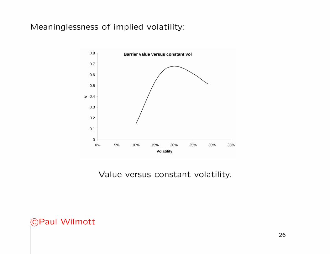
Meaninglessness of implied volatility:
Barrier value versus constant vol
0
0.1
0.2
0.3
0.4
0.5
0.6
0.7
0.8
0% 5% 10% 15% 20% 25% 30% 35%
Volatility
V
Value versus constant volatility.
c©Paul Wilmott
26

Lesson 5: Correlation
• Quant toolbox
When we think of two assets that are highly correlated then we
are tempted to think of them both moving along side by side
almost. Surely if one is growing rapidly then so must the other?
This is not true.
c©Paul Wilmott
27

Perfect positive correlation
0
5
10
15
20
25
30
35
40
0 5 10 15 20 25 30
Time
Ass
et v
alu
e
AB
Two perfectly correlated assets.
c©Paul Wilmott
28
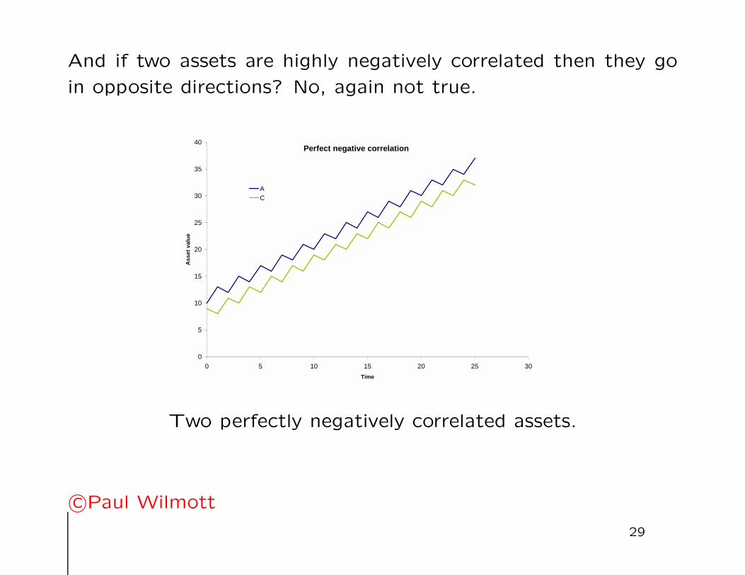
And if two assets are highly negatively correlated then they go
in opposite directions? No, again not true.
Perfect negative correlation
0
5
10
15
20
25
30
35
40
0 5 10 15 20 25 30
Time
Ass
et v
alu
eAC
Two perfectly negatively correlated assets.
c©Paul Wilmott
29

If we are modelling using stochastic differential equations thencorrelation is about what happens at the smallest, technicallyinfinitesimal, timescale. It is not about the ‘big picture’ direction.This can be very important and confusing. For example, if weare interested in how assets behave over some finite time horizonthen we still use correlation even though we typically don’t careabout short timescales only our longer investment horizon (atleast in theory).
However, if we are hedging an option that depends on two ormore underlying assets then, conversely, we don’t care aboutdirection (because we are hedging), only about dynamics overthe hedging timescale. The use of correlation may then be easierto justify. But then we have to ask how stable is this correlation.
So when wondering whether correlation is meaningful in anyproblem you must answer two questions (at least), one con-cerning timescales (investment horizons or hedging period) andanother about stability.
c©Paul Wilmott
30
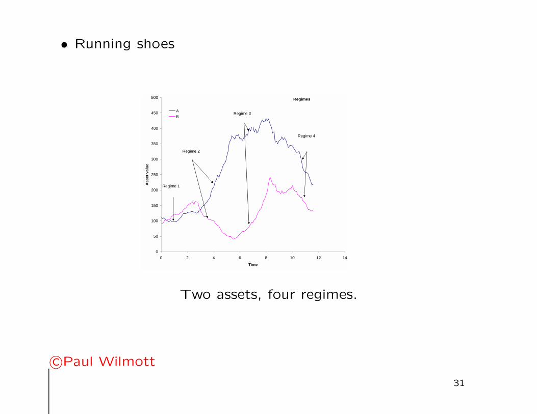
• Running shoes
Regimes
0
50
100
150
200
250
300
350
400
450
500
0 2 4 6 8 10 12 14
Time
Ass
et v
alu
e
A
B
Regime 1
Regime 2
Regime 3
Regime 4
Two assets, four regimes.
c©Paul Wilmott
31
As you can see, the dynamics between just two companies can
be fascinating. And can be modelled using all sorts of interesting
mathematics. One thing is for sure and that is such dynamics
while fascinating are certainly not captured by a correlation of
0.6!
c©Paul Wilmott
32

Example: Synthetic CDOs suffer from problems with correla-
tion. People typically model these using a copula approach, and
then argue about which copula to use. Finally because there
are so many parameters in the problem they say “Let’s assume
they are all the same!” Then they vary that single constant
correlation to look for sensitivity (and to back out implied cor-
relations). Where do I begin criticizing this model? Let’s say
that just about everything in this model is stupid and dangerous.
The model does not capture the true nature of the interaction
between underlyings, correlation never does, and then making
such an enormously simplifying assumption about correlation is
just bizarre. (I grant you not as bizarre as the people who lap
this up without asking any questions.)
c©Paul Wilmott
33

Synthetic CDO
-
10
20
30
40
50
60
70
80
90
0% 5% 10% 15% 20% 25% 30% 35% 40% 45%
Correlation
Pri
ce
Equity tranche 0-3%
Junior 3-6%
Mezzanine 6-9%
Mezzanine 9-12%
Various tranches versus correlation.
c©Paul Wilmott
34

Lesson 6: Reliance on Continuous Hedging (Arguments)
One of the most important concepts in quantitative finance is
that of delta or dynamic hedging. This is the idea that you can
hedge risk in an option by buying and selling the underlying asset.
This is called delta hedging since ‘delta’ is the Greek letter used
to represent the amount of the asset you should sell. Classical
theories require you to rebalance this hedge continuously. In
some of these theories, and certainly in all the most popular,
this hedging will perfectly eliminate all risk. Once you’ve got rid
of risk from your portfolio it is easy to value since it should then
get the same rate of return as putting money in the bank.
c©Paul Wilmott
35
This is a beautiful, elegant, compact theory, with lots of impor-
tant consequences. Two of the most important consequences
(as well as the most important which is. . . no risk!) are that,
first, only volatility matters in option valuation, the direction of
the asset doesn’t, and, second, if two people agree on the level
of volatility they will agree on the value of an option, personal
preferences are not relevant.
The assumption of continuous hedging seems to be crucial to
this theory. But is this assumption valid?
c©Paul Wilmott
36

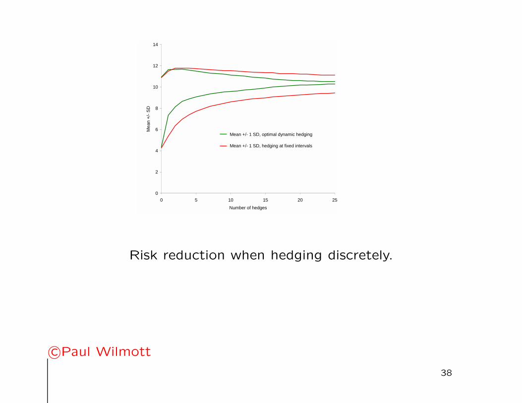
The figure shows a comparison between the values of an at-the-
money call, strike 100, one year to expiration, 20% volatility,
5% interest rate, when hedged at fixed intervals (the red line)
and hedged optimally (the green line). The lines are the mean
value plus and minus one standard deviation. All curves con-
verge to the Black-Scholes complete-market, risk-neutral, price
of 10.45, but hedging optimally gets you there much faster. If
you hedge optimally you will get as much risk reduction from
just 10 rehedges as if you use 25 equally spaced rehedges.
c©Paul Wilmott
37
0
2
4
6
8
10
12
14
0 5 10 15 20 25
Number of hedges
Mea
n +
/- S
D
Mean +/- 1 SD, optimal dynamic hedging
Mean +/- 1 SD, hedging at fixed intervals
Risk reduction when hedging discretely.
c©Paul Wilmott
38
From this we can conclude that as long as people know the best
way to dynamically hedge then we may be able to get away with
using risk neutrality even though hedging is not continuous.
But do they know this?
Everyone is brought up on the results of continuous hedging, and
they rely on them all the time, but they almost certainly do not
have the necessary ability to make those results valid!
c©Paul Wilmott
39
Lesson 7: Feedback
Are derivatives a good thing or a bad thing? Their origins are
in hedging risk, allowing producers to hedge away financial risk
so they can get on with making pork bellies or whatever. Now
derivatives are used for speculation, and the purchase/sale of
derivatives for speculation outweighs their use for hedging.
Does this matter? We know that speculation with linear forwards
and futures can affect the spot prices of commodities, especially
in those that cannot easily be stored. But what about all the
new-fangled derivatives that are out there?
c©Paul Wilmott
40

A simplistic analysis would suggest that derivatives are harmless,
since for every long position there is an equal and opposite short
position, and they cancel each other out. But this misses the
important point that usually one side or the other is involved in
some form of dynamic hedging used to reduce their risk. Often
one side buys a contract so as to speculate on direction of the
underlying. The seller is probably not going to have exactly the
opposite view on the market and so they must hedge away risk
by dynamically hedging with the underlying. And that dynamic
hedging using the underlying can move the market. This is the
tail wagging the dog!
c©Paul Wilmott
41

There are two famous examples of this feedback effect:
• Convertible bonds—volatility decrease
• 1987 crash and (dynamic) portfolio insurance—volatility in-
crease
c©Paul Wilmott
42
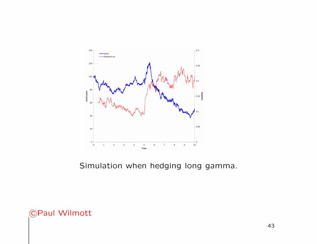
0
20
40
60
80
100
120
140
0 1 2 3 4 5 6 7 8 9 10
Time
Ass
et p
rice
0
0.05
0.1
0.15
0.2
0.25
0.3
Vo
lati
lity
Asset
Realized vol
Simulation when hedging long gamma.
c©Paul Wilmott
43

0
20
40
60
80
100
120
140
0 1 2 3 4 5 6 7 8 9 10
Time
Ass
et p
rice
0
0.1
0.2
0.3
0.4
0.5
0.6
0.7
0.8
Vo
lati
lity
Asset
Realized vol
Simulation when hedging short gamma.
c©Paul Wilmott
44

Lesson 8: Reliance on Closed-form Solutions
Example: You need to value a fixed-income contract and so
you have to choose a model. Do you (a) analyze historical fixed-
income data in order to develop an accurate model, this is then
solved numerically, and finally back tested using a decade’s worth
of past trades to test for robustness, or (b) use Professor X’s
model because the formulæ are simple and, quite frankly, you
don’t know any numerical analysis, or (c) do whatever everyone
else is doing? Typically people will go for (c), partly for reasons
already discussed, which amounts to (b).
c©Paul Wilmott
45

Example: You are an aeronautical engineer designing a new
airplane. Boy, those Navier–Stokes equations are hard! How do
you solve non-linear equations? Let’s simplify things, after all
you made a paper plane as a child, so let’s just scale things up.
The plane is built, a big engine is put on the front, it’s filled
with hundreds of passengers, and it starts its journey along the
runway. You turn your back, without a thought for what happens
next, and start on your next project.
One of those examples is fortunately not real. Unfortunately, the
other is.
c©Paul Wilmott
46

Quants love closed-form solutions. The reasons are
1. Pricing is faster
2. Calibration is easier
3. You don’t have to solve numerically
c©Paul Wilmott
47
Popular examples of closed-form solutions/models are, in equityderivatives, the Heston stochastic volatility model, and in fixedincome, Vasicek,∗ Hull & White, etc.
Models with closed-form solutions have several roles in quanti-tative finance. Closed-form solutions are
• useful for preliminary insight
• good for testing your numerical scheme before going on tosolve the real problem
• for examining second-year undergraduate mathematicians
c©Paul Wilmott∗To be fair to Vasieck I’m not sure he ever claimed he had a great model,his paper set out the general theory behind the spot-rate models, with whatis now known as the Vasicek model just being an example.
48

Lesson 9: Valuation is Not Linear
You want to buy an apple, so you pop into Waitrose. An apple
will cost you 50p. Then you remember you’ve got friends coming
around that night and these friends really adore apples. Maybe
you should buy some more? How much will 100 apples cost?
c©Paul Wilmott
49

Here’s a quote from a well-known book: “The change of nu-
meraire technique probably seems mysterious. Even though one
may agree that it works after following the steps in the chapter,
there is probably a lingering question about why it works. The
author’s opinion is that it may be best simply to regard it as a
‘computational trick’. Fundamentally it works because valuation
is linear. . . . The linearity is manifested in the statement that
the value of a cash flow is the sum across states of the world of
the state prices multiplied by the size of the cash flow in each
state. . . . After enough practice with it, it will seem as natural
as other computational tricks one might have learned.”
Note it doesn’t say that linearity is an assumption, it is casually
taken as a fact. Valuation is apparently linear. Now there’s
someone who has never bought more than a single apple!
c©Paul Wilmott
50

Example: The same author may be on a sliding royalty scale so
that the more books he sells the bigger his percentage. How can
nonlinearity be a feature of something as simple as buying apples
or book royalties yet not be seen in supposedly more complex
financial structured products?
c©Paul Wilmott
51

Example: A bank makes a million dollars profit on CDOs.
Fantastic! Let’s trade 10 times as much! They make $10mil-
lion profit. The bank next door hears about this and decides
it wants a piece of the action. They trade the same size. Be-
tween the two banks they make $18million profit. Where’d the
$2million go? Competition between them brings the price and
profit margin down. To make up the shortfall, and because of
simple greed, they increase the size of the trades. Word spreads
and more banks join in. Profit margins are squeezed. Total
profit stops rising even though the positions are getting bigger
and bigger. And then the inevitable happens, the errors in the
models exceed the profit margin (margin for error), and between
them the banks lose billions. “Fundamentally it works because
valuation is linear.” Oh dear!
c©Paul Wilmott
52
To appreciate the importance of nonlinearity you have to under-
stand that there is a difference between the value of a portfolio
of contracts and the sum of the values of the individual con-
tracts.∗ In pseudomath, if the problem has been set up properly,
you will get
Value(A + B) ≥ Value(A) + Value(B).
c©Paul Wilmott
∗What I call, to help people remember it, the ‘Beatles effect.’ The Fab Fourbeing immeasurably more valuable as a group than as individuals. . . Wings,Thomas the Tank Engine,. . .
53

• Static hedging of a barrier option
c©Paul Wilmott
54
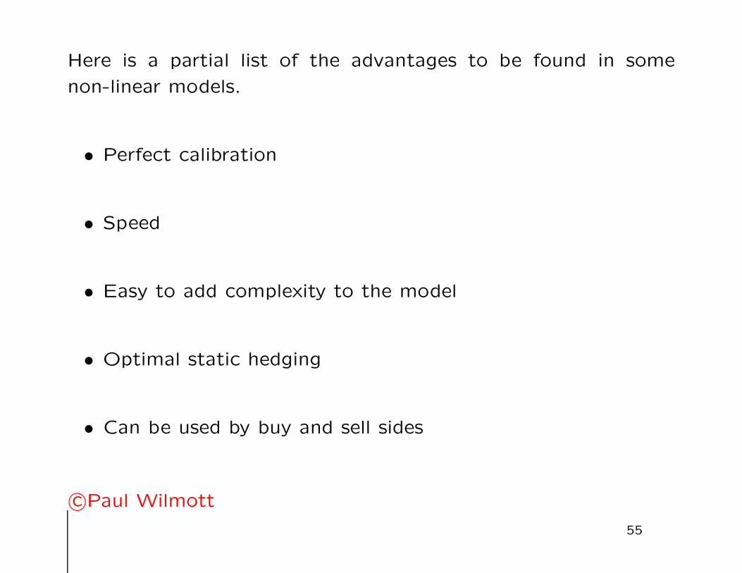
Here is a partial list of the advantages to be found in some
non-linear models.
• Perfect calibration
• Speed
• Easy to add complexity to the model
• Optimal static hedging
• Can be used by buy and sell sides
c©Paul Wilmott
55
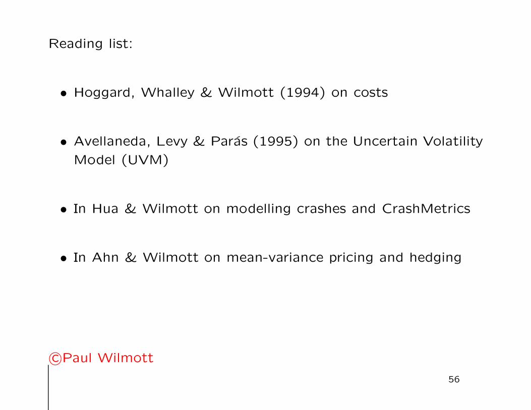
Reading list:
• Hoggard, Whalley & Wilmott (1994) on costs
• Avellaneda, Levy & Paras (1995) on the Uncertain Volatility
Model (UVM)
• In Hua & Wilmott on modelling crashes and CrashMetrics
• In Ahn & Wilmott on mean-variance pricing and hedging
c©Paul Wilmott
56

Lesson 10: Calibration
“A cynic is a man who knows the price of everything and the
value of nothing,” said Oscar Wilde.
Example: Wheels cost $10 each. A soapbox is $20. How much
is a go-cart? The value is $60.
Price?
Worth?
c©Paul Wilmott
57
• The WWVN
c©Paul Wilmott
58
• inverse problems
• frozen fish
• CSI Miami
• crystal balls
c©Paul Wilmott
59

Problems with calibration:
• Over fitting. You lose important predictive information if
your model fits perfectly. The more instruments you calibrate
to the less use that model is.
• Fudging hides model errors: Perfect calibration makes you
think you have no model risk, when in fact you probably
have more than if you hadn’t calibrated at all.
• Always unstable. The parameters or surfaces always change
when you recalibrate.
• Confusion between actual parameter values and those seen
via derivatives. For example there are two types of credit
risk, the actual risk of default and the market’s perceived
risk of default.
c©Paul Wilmott
60

Why is calibration unstable?
• Market Price of Risk
c©Paul Wilmott
61

Lambda
-20
-15
-10
-5
0
5
01/01/1982 04/06/1985 05/11/1988 08/04/1992 10/09/1995 11/02/1999 15/07/2002 16/12/2005
FEAR
GREED
Market price of interest rate risk versus time.
c©Paul Wilmott
62

When you calibrate you are saying that whatever the market
sentiment is today, as seen in option prices, is going to pertain
forever. So if the market is panicking today it will always panic.
But the figure shows that such extremes of emotion are short-
lived. And so if you come back a week later you will now be
calibrating to a market that has ceased panicking and is perhaps
now greedy!
Calibration assumes a structure for the future that is inconsistent
with experience, inconsistent with common sense, and that fails
all tests.
c©Paul Wilmott
63

Lesson 11: Too much precision
Given all the errors in the models, their unrealistic assumptions,
and the frankly bizarre ways in which they are used, it is surprising
that banks and funds make money at all!
• Zero sum
• Who owns the world
c©Paul Wilmott
64
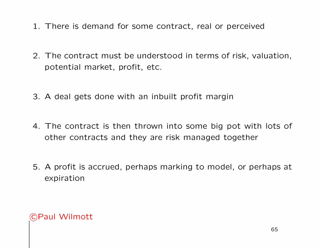
1. There is demand for some contract, real or perceived
2. The contract must be understood in terms of risk, valuation,
potential market, profit, etc.
3. A deal gets done with an inbuilt profit margin
4. The contract is then thrown into some big pot with lots of
other contracts and they are risk managed together
5. A profit is accrued, perhaps marking to model, or perhaps at
expiration
c©Paul Wilmott
65
Stages 2 and 4 are inconsistent.
c©Paul Wilmott
66

The point of this lesson is to suggest that more effort is spent
on the benefits of portfolios than on fiddly niceties of modelling
to an obsessive degree of accuracy. Accept right from the start
that the modelling is going to be less than perfect. It is not true
that one makes money from every instrument because of the
accuracy of the model. Rather one makes money on average
across all instruments despite the model. These observations
suggest to me that less time should be spent on dodgy mod-
els, meaninglessly calibrated, but more time on models that are
accurate enough and that build in the benefits of portfolios.
c©Paul Wilmott
67
Some models are better than others. Sometimes even working
with not-so-good models is not too bad. To a large extent what
determines the success of models is the type of market. Let me
give some examples.
Equity, FX and commodity markets: Here the models are
only so-so. There has been a great deal of research on im-
proving these models, although not necessarily productive work.
Combine less-than-brilliant models with potentially very volatile
markets and exotic, non-transparent, products and the result can
be dangerous. On the positive side as long as you diversify across
instruments and don’t put all your money into one basket then
you should be ok.
c©Paul Wilmott
68

Fixed-income markets: These models are pretty dire. So you
might expect to lose (or make) lots of money. Well, it’s not
as simple as that. There are two features of these markets
which make the dire modelling less important, these are a) the
underlying rates are not very volatile and b) there are plenty of
highly liquid vanilla instruments with which to try to hedge model
risk. (I say “try to” because most model-risk hedging is really a
fudge, inconsistent with the framework in which it is being used.)
c©Paul Wilmott
69

Correlation markets: Oh, Lord! Instruments whose pricing
requires input of correlation (FI excepted, see above) are acci-
dents waiting to happen. The dynamic relationship between just
two equities can be beautifully complex, and certainly never to
be captured by a single number, correlation. Fortunately these
instruments tend not to be bought or sold in non-diversified,
bank-destroying quantities. (Except for CDOs, of course!)
c©Paul Wilmott
70
Credit markets: Single-name instruments are not too bad.
Again problems arise with any instrument that has multiple ‘un-
derlyings,’ so the credit derivatives based on baskets. . . you know
who you are. But as always, as long as the trades aren’t too big
then it’s not the end of the world.
c©Paul Wilmott
71
Lesson 12: Too Much Complexity
“Four stochastic parameters good, two stochastic parameters
bad.” (Thanks to George Orwell.)
• Selling books to non mathematicians
• Impressing people (books with yellow covers)
c©Paul Wilmott
72

• 30 pages or 4 pages (Hyungsok Ahn)
• Rule 1 of quant finance seems to be ‘Make this as difficult
as we can.’
• Brainteaser on wilmott.com: Girsanov, Doleans-Dade mar-
tingales, and optimal stopping
c©Paul Wilmott
73

Bonus Lesson 13: The Binomial Method is Rubbish
I really like the binomial method. But only as a teaching aid. Itis the easiest way to explain
1. hedging to eliminate risk
2. no arbitrage
3. risk neutrality
I use it in the CQF to explain these important, and sometimesdifficult to grasp, concepts.∗ But once the CQFers have un-derstood these concepts they are instructed never to use thebinomial model again, on pain of having their CQFs withdrawn!
c©Paul Wilmott
∗It’s also instructive to also take a quick look at the trinomial version, becausethen you see immediately how difficult it is to hedge in practice.
74

The binomial model was the first of what are now known as
finite-difference methods. It dates back to 1911 and was the
creation of Lewis Fry Richardson, all-round mathematician, so-
ciologist, and poet.
Things have come on a long way since 1911.
c©Paul Wilmott
75

A lot of great work has been done on the development of these
numerical methods in the last century. But very little has been
done, relatively speaking, on the development of the binomial
model. The binomial model is finite differences with one hand
tied behind its back, hopping on one leg, while blindfolded.
• Lazy professors and their lecture notes
And so generations of students are led to believe that the bino-
mial method is state of the art when it is actually prehistoric.
c©Paul Wilmott
76
Summary
Question 1: What are the advantages of diversification among
products, or even among mathematical models?
Answer 1: No advantage to your pay whatsoever!
Question 2: If you add risk and curvature what do you get?
Answer 2: Value!
Question 3: If you increase volatility what happens to the value
of an option?
Answer 3: It depends on the option!
c©Paul Wilmott
77

Question 4: If you use ten different volatility models to value
an option and they all give you very similar values what can you
say about volatility risk?
Answer 4: You may have a lot more than you think!
Question 5: One apple costs 50p, how much will 100 apples
cost you?
Answer 5: Not £50!
c©Paul Wilmott
78
QF is interesting and challenging, not because the mathematics
is complicated, it isn’t, but because putting maths and trading
and market imperfections and human nature together and trying
to model all this, knowing all the while that it is probably futile,
now that’s fun!
c©Paul Wilmott
79
References
Ahmad, R & Wilmott, P 2005 Which free lunch would you like today, Sir?Delta hedging, volatility arbitrage and optimal portfolios. Wilmott magazineNovember 64–79
Ahmad, R & Wilmott, P 2007 The market price of interest rate risk: Mea-suring and modelling fear and greed in the fixed-income markets. Wilmottmagazine, January
Ahn, H & Wilmott, P 2003 Stochastic volatility and mean-variance analysis.Wilmott magazine November 2003 84–90
Ahn, H & Wilmott, P 2007 Jump Diffusion, Mean and Variance: How toDynamically Hedge, Statically Hedge and to Price. Wilmott magazine May2007 96–109
Ahn, H & Wilmott, P 2008 Dynamic Hedging is Dead! Long Live StaticHedging! Wilmott magazine January 2008 80–7
Avellaneda, M, Levy, A & Paras, A 1995 Pricing and hedging derivative se-curities in markets with uncertain volatilities. Applied Mathematical Finance2 73–88
Avellaneda, M & Paras, A 1996 Managing the volatility risk of derivative se-curities: the Lagrangian volatility model. Applied Mathematical Finance 321–53
c©Paul Wilmott
80
Avellaneda, M & Buff, R 1997 Combinatorial implications of nonlinear uncer-tain volatility models: the case of barrier options. Courant Institute, NYU
Derman, E & Kani, I 1994 Riding on a smile. Risk magazine 7 (2) 32–39(February)
Dupire, B 1993 Pricing and hedging with smiles. Proc AFFI Conf, La BauleJune 1993
Dupire, B 1994 Pricing with a smile. Risk magazine 7 (1) 18–20 (January)
Haug, EG 2007 Complete Guide to Option Pricing Formulas. McGraw–Hill
Ho, T & Lee, S 1986 Term structure movements and pricing interest ratecontingent claims. Journal of Finance 42 1129–1142
Hoggard, T, Whalley, AE & Wilmott, P 1994 Hedging option portfolios inthe presence of transaction costs. Advances in Futures and Options Research7 21–35
Hua, P & Wilmott, P 1997 Crash courses. Risk magazine 10 (6) 64–67(June)
Hua, P & Wilmott, P 1998 Value at risk and market crashes. DerivativesWeek
Hua, P & Wilmott, P 1999 Extreme scenarios, worst cases, CrashMetrics andPlatinum Hedging. Risk Professional
Hua, P & Wilmott, P 2001 CrashMetrics. In New Directions in MathematicalFinance. (Eds P.Wilmott and H.Rasmussen.)
c©Paul Wilmott
81

Hull, JC & White, A 1990 Pricing interest rate derivative securities. Reviewof Financial Studies 3 573–592
Schonbucher, PJ & Wilmott, P 1995 Hedging in illiquid markets: nonlineareffects. Proceedings of the 8th European Conference on Mathematics in In-dustry
Schoutens, W, Simons, E & Tistaert, J 2004 A perfect calibration! Nowwhat? Wilmott magazine March 2004 66–78
Rubinstein, M 1994 Implied binomial trees. Journal of Finance 69 771–818
Vasicek, OA 1977 An equilibrium characterization of the term structure. Jour-nal of Financial Economics 5 177–188
Whalley, AE & Wilmott, P 1993 a Counting the costs. Risk magazine 6 (10)59–66 (October)
Whalley, AE & Wilmott, P 1993 b Option pricing with transaction costs.MFG Working Paper, Oxford
Whalley, AE & Wilmott, P 1994 a Hedge with an edge. Risk magazine 7(10) 82–85 (October)
Whalley, AE & Wilmott, P 1994 b A comparison of hedging strategies. Pro-ceedings of the 7th European Conference on Mathematics in Industry 427–434
c©Paul Wilmott
82
Whalley, AE & Wilmott, P 1995 An asymptotic analysis of the Davis, Panasand Zariphopoulou model for option pricing with transaction costs. MFGWorking Paper, Oxford University
Whalley, AE & Wilmott, P 1996 Key results in discrete hedging and trans-action costs. In Frontiers in Derivatives (Ed. Konishi, A and Dattatreya, R.)183–196
Whalley, AE & Wilmott, P 1997 An asymptotic analysis of an optimal hedg-ing model for option pricing with transaction costs. Mathematical Finance 7307–324
Wilmott, P 2002 Cliquet options and volatility models. Wilmott magazineDecember 2002
Wilmott, P 2006a Paul Wilmott On Quantitative Finance, second edition.John Wiley and Sons
Wilmott, P 2006b Frequently Asked Questions in Quantitative Finance. JohnWiley and Sons
c©Paul Wilmott
83