Where Juvenile Serious Offenders Live: A Neighborhood ...WHERE JUVENILE SERIOUS OFFENDERS LIVE: A...

WHERE JUVENILE SERIOUS OFFENDERS LIVE: A NEIGHBORHOOD ANALYSIS

OF WAYNE COUNTY, MICHIGAN

Irene Y.H. Ng

Department of Social Work

National University of Singapore

AS 3 Level 4, 3 Arts Link

Singapore 117570

Singapore

Tel: (65) 6516-6050, Fax: (65) 6778-1213, E-mail: [email protected]

of 41

1

WHERE JUVENILE SERIOUS OFFENDERS LIVE: A NEIGHBORHOOD ANALYSIS

OF WAYNE COUNTY, MICHIGAN

Abstract: This article studies the relationship between neighborhood factors and

juvenile serious offenders in Wayne County, Michigan. This is where Detroit is, a city

with a glorious past but a bleak future. Administrative data are linked to tract-level

census characteristics that proxy for social disorganization structural factors. Results by

negative binomial regressions found significant associations in the expected direction

with concentrated disadvantage, concentrated affluence, and inequality. However,

concentrated immigration is insignificantly related to juvenile serious offending and

residential stability increases rather than decreases offending. These counter-theoretical

results may be due to the presence of homes to students and young professionals and

vibrant Latino immigrant communities. The stark contrasts documented by the analysis

and the high correlation of economic conditions to juvenile crime demand urgent and

radical responses to completely transform impoverished neighborhoods in Wayne

County.

Keywords: juvenile serious offending, Detroit, neighborhood

of 41

2

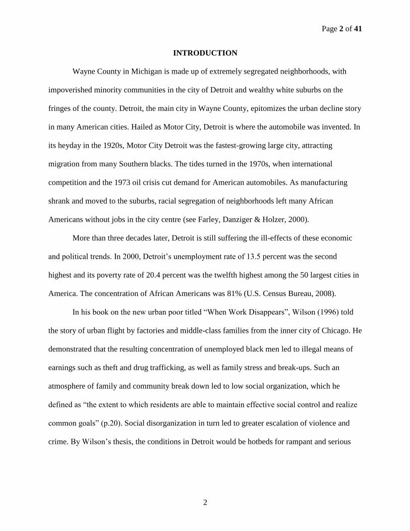
INTRODUCTION

Wayne County in Michigan is made up of extremely segregated neighborhoods, with

impoverished minority communities in the city of Detroit and wealthy white suburbs on the

fringes of the county. Detroit, the main city in Wayne County, epitomizes the urban decline story

in many American cities. Hailed as Motor City, Detroit is where the automobile was invented. In

its heyday in the 1920s, Motor City Detroit was the fastest-growing large city, attracting

migration from many Southern blacks. The tides turned in the 1970s, when international

competition and the 1973 oil crisis cut demand for American automobiles. As manufacturing

shrank and moved to the suburbs, racial segregation of neighborhoods left many African

Americans without jobs in the city centre (see Farley, Danziger & Holzer, 2000).

More than three decades later, Detroit is still suffering the ill-effects of these economic

and political trends. In 2000, Detroit’s unemployment rate of 13.5 percent was the second

highest and its poverty rate of 20.4 percent was the twelfth highest among the 50 largest cities in

America. The concentration of African Americans was 81% (U.S. Census Bureau, 2008).

In his book on the new urban poor titled “When Work Disappears”, Wilson (1996) told

the story of urban flight by factories and middle-class families from the inner city of Chicago. He

demonstrated that the resulting concentration of unemployed black men led to illegal means of

earnings such as theft and drug trafficking, as well as family stress and break-ups. Such an

atmosphere of family and community break down led to low social organization, which he

defined as “the extent to which residents are able to maintain effective social control and realize

common goals” (p.20). Social disorganization in turn led to greater escalation of violence and

crime. By Wilson’s thesis, the conditions in Detroit would be hotbeds for rampant and serious

of 41

3

crimes. Indeed, the violent crime rate in Detroit in 2000 was 23 per 1,000 inhabitants, the

seventh highest in the nation (Federal Bureau of Investigation, n.d.-a).

Several other crime ecology studies have documented the adverse consequences of

neighborhood structures on crime. Besides relating structural conditions directly with crime and

delinquency, many studies took a step further to model the mediation of social processes

between structural conditions and final outcomes (e.g. Martin, 2002; Morenoff, Sampson &

Raudenbush, 2001; Sampson, Raudenbush & Earls, 1997). With data at neighborhood as well as

individual levels, research has also been able to use multilevel models to establish neighborhood

effects on individual offending independent of individual characteristics such as age, sex,

socioeconomic status (SES), and prior offending (e.g. Gottfredson, McNeil III & Gottfredson,

1991). The empirical evidence from these studies is clear: neighborhood socioeconomic

conditions are strongly associated with offending, even after controlling for individual

characteristics. For example, Gottfredson et al. found that significantly fewer adolescent males

who lived in more affluent and educated neighborhoods self-reported theft and vandalism, after

controlling for individual and social factors such as peer influence, parental supervision and

school attachment. Sampson and colleagues explicitly modeled the link between structural

factors (such as concentrated disadvantage and residential stability) and crime through a social

process they called collective efficacy, defined as “social cohesion among neighbors combined

with their willingness to intervene on behalf of the common good” (Sampson et al., 1997). They

found that collective efficacy mediated a substantial portion of the association between structural

factors and crime outcomes such as homicide and violent victimization. Nevertheless, some

significant effects of structural factors on crime remain (e.g. Morenoff et al., 2001; Sampson et

al., 1997; Sampson, 1999).

of 41

4

These neighborhood effects studies have hailed mostly from Chicago (e.g. the collective

efficacy studies of Sampson and colleagues, and Wilson’s collection on the urban poor). Crime

ecology research on the Detroit area is more limited. Gyimah-Brempong (2001) related density

of stores selling alcohol to crime. Bergmann (2008) followed the lives of two young drug dealers

in Detroit. Martin (2002) might be closest in methodology to this study. He found that greater

concentrated poverty, lower social capital, and greater residential stability were correlated with

higher burglary rates in Detroit. Others are either dated or focused on employment opportunities

or social services.

This article studies whether and what neighborhood variables are related to juvenile

serious offending in Wayne County in Michigan. Compared to the hierarchical methods

employed in the existing studies which nest individual level variables within neighborhood

variables, this study is limited because only aggregate level variables are available as correlates

of youth serious offending. With data only from the Census and limited juvenile offender data

from the State, this study also examines only structural variables without considering social

mediators. Despite the above data limitations, though, given the limited neighborhood research

on Detroit and Wayne County, the findings here can offer important crime prevention and

community rehabilitation applications for an area in dire need. Using the social disorganization

theories as framework, this study provides a test of whether and how the structural variables that

have been identified through existing area studies pan out in Wayne County. Does the story in

Wayne County support findings in other parts of the United States? Or do particular

characteristics in Wayne County yield results that diverge from other findings? The study also

offers insight into serious crimes by young males, the type of crime which social disorganization

theories claim to explain.

of 41

5

The rest of the article progresses as follows. The next section explains the social

disorganization framework used in the analysis. The framework informs the empirical model,

which is discussed next with an outline of the independent variables, an explanation of how the

dependent variable - juvenile serious offending rates – is constructed, and the analytical strategy.

The findings section first show the descriptive contrast of neighborhoods in Wayne through a

comparison with the rest of Michigan and the U.S. Then, it presents the multivariate results from

negative binomial regressions. Due to the high number of neighborhoods with no serious youth

offenders, negative binomial regression corrects for the over dispersion of zeroes. This gets

around the specification problem of OLS, which requires an assumption of normality. The article

closes with a discussion of the implications of the findings for intervention and future research.

THE SOCIAL DISORGANIZATION FRAMEWORK

This study follows the social disorganization framework first adopted by Shaw and

McKay (1942) and further developed by others such as Wilson (1987, 1996), and Sampson and

colleagues (e.g. Sampson, Morenoff & Earls, 1999; Sampson et. al., 1997; Sampson & Wilson,

1995). In terms of specification of an empirical model, Sampson et al. (1999) (SME) applied four

structural factors of disorganization that they termed as structural antecedents. First, following

Wilson (1996, 1978), where the problems of family breakdown, ethnic concentration, poverty

and unemployment are intertwined with the flight of industries and middle-class whites from

urban centers, it might be important to operationalize an index of concentrated disadvantage that

combines economic as well as the social disadvantages of family structure and ethnic minority

status. Second, following Coleman’s (1988, 1990) theory of continuity of community structure,

SME suggested that “a high rate of residential turnover, especially population loss, fosters

of 41

6

institutional disruption and weakens interpersonal ties” (p.636). Homeowners, in particular, have

the shared interest to support neighborhood networks. This problem of transitional residents was

also highlighted in Shaw and McKay (1942). Third, concentration of immigrant groups might

have a separate effect on neighborhood disorganization “because of linguistic barriers and

cultural isolation” (p.637). Fourth, with results from Brooks-Gunn et al. (1993) showing positive

effects of concentrated socioeconomic advantage on children, SME also suggested including a

measure of concentrated affluence that reflect high socio-economic status in terms of earnings,

occupation, and education.

Contrary to the predictions of social disorganization theories, however, Nielsen, Martinez

and Rosenfeld (2005) suggested that the effects of residential instability and immigration

concentration depend on local contexts. In their study of Miami and San Diego, they found that

neighborhoods with higher immigrant concentration had lower homicide rates in Miami, but had

higher drug-related homicide rates in San Diego. Nielsen et al. explained that the differing results

could be because San Diego had lower social capital levels and more segmented assimilation

than Miami. In Miami, the immigrant revitalization perspective of Lee and Martinez (2002)

might apply, where immigrants stabilize or revitalize neighborhoods when they have

opportunities to be incorporated into the economic structure.

What can we expect in the case of Detroit and Wayne County? The Southwest of Detroit,

for example, has the largest concentration of Hispanics/Latinos in Michigan, and the numbers are

increasing. “Hispanics are the fastest growing ethnicity in Detroit, having increased in population

by 66 percent between 1990 and 2000” (Center for Urban Studies (CUS) & Skillman Center for

Children, 2004). In contrast, Detroit lost 0.28 percent of its African-American population during

the same period (U.S. Census Bureau, 2008). A 2008 CUS Report on Hispanics in Southeast

of 41

7

Michigan showed their increasing contribution to the economy but their continued lag in

educational standard. In a 2001 report, CUS asserted that “the impact on areas receiving large

numbers of immigrants will be positive because of the value new immigrants place on family,

education, entrepreneurial activity, and the work ethic” (p.4). The findings in these reports imply

that the predominantly Latino neighborhoods might have experienced some revival compared to

predominantly black neighborhoods. Relative to homogeneously white neighborhoods, however,

neighborhoods with high immigrant populations might still be worse off.

Similarly, residential stability in Wayne County might not relate to crime in the way

posited by social disorganization. While it is generally true that the less well off in Wayne

County tend to be renters and many people move within and out of the county, some of the most

disadvantaged neighborhoods may have home owners who were stuck in the inner city. At the

other end, some revitalization efforts have also resulted in the development of rental units to

young professionals near the commercial center and to university students of Wayne State

University. Also, immigrant populations tend to be renters, and it has been asserted above that

immigrant communities might inject more social order than predominantly black communities.

Therefore, results on immigrants and residents in Wayne County might go in the opposite

direction from predictions of social disorganization. Besides Nielsen et al., some other studies

have also found such opposite effects. Sampson et al. (1997) found that immigration does not

affect homicide and residential stability increases rather than decreases homicide. Morenoff et al.

(2001) obtained significant positive associations for residential stability and concentrated

immigration with incident-based but not victim-based homicide rates. Closer to home, Martin

(2002) found residential stability related to higher burglary rates.

of 41

8

Besides the above four structural factors in SME, some recent research has also

considered effects of inequality (e.g. Kubrin and Stewart, 2006; Smith et al., 2000). Hipp (2007)

suggested that both inequality and racial/ethnic heterogeneity increase social distances and

therefore decrease social interactions within the community, which then lead to lower social

control.

DATA AND METHODOLOGY

INDEPENDENT VARIABLES

Based on the above social disorganization framework, the empirical model in this paper

applies the four “structural antecedents” in SME and a measure of inequality. Two specifications

are analyzed. The first specification simply applies the four SME indices with an interaction term

to signify inequality. The second specification includes the variables in the indices individually

in order to identify what variables are driving the results.

The first scale, concentrated disadvantage (CD, =.77), comprises percent below poverty

line, percent receiving public assistance (PA), percent unemployed, percent single female-headed

families with children, and percent black. Two variables contribute to the second scale,

concentrated immigration (CI, =.64): percent Latino and percent foreign-born. Specifically,

then, it is measuring concentrated Latino immigration. The third scale, residential stability (RS,

=.58) includes percent of residents five years old and above who resided in the same house five

years earlier, and the percent of owner-occupied homes. Included in the fourth scale,

concentrated affluence (CA, =.88), are the percent of families with incomes higher than

$75,000, the percent of adults with college education, and the percent of professionals and

managers among those in the civilian labor force.

of 41

9

Factor analysis of the above census variables used in SME on the Wayne data indeed

yielded the same four separate scales. The results in Table 1 with one varimax rotation show the

high loadings and separation into each factor. Although percent occupied housing loaded highly

on factor 1, which gives the CD items, the decision was made to follow SME and use it with

percent who lived in the same house in the past five years to make the RS scale.

The final factor is inequality. The index of Concentration at the Extremes (ICE) by

Massey (2001) has been used as a measure of relative inequality (e.g. Morenoff et al., 2001;

Kubrin and Stewart, 2006). ICE is given by the difference between the number of rich families

and the number of poor families, divided by the total number of families. The range of this index

is then from -1 when all families are poor to 1 when all families are rich. While it measures the

proportional balance between affluence and poverty, it does not represent inequality per se.

Consider two extreme types of neighborhoods: one where half the families are extremely rich

and the other half are extremely poor, and one where all are middle income. Both neighborhoods

will have an ICE magnitude of zero. However, while the former neighborhood is extremely

unequal, the latter neighborhood is completely equal. Estimates from ICE show the effect of

inequality only while holding CD constant. This inequality can be more simply and directly

accounted for by interacting CD with CA. A positive coefficient from the interaction would

imply that a higher percentage of wealthy households increases the criminogenic effects of

greater economic disadvantage and vice versa. This will support social disorganization theories.

To capture effects of ethnic/racial heterogeneity, the analysis switches to a different

specification where all the variables used to construct the above scales were used as individual

variables. In this variable-by-variable specification, inequality is measured by interacting percent

poor with percent above $75,000. Similarly, following Smith, Frazee and Davison (2000) and

of 41

10

Miethe and McDowall (1993), racial heterogeneity can be expressed as the product between the

proportion African American and the proportion Whites. Due to the trends in Latino immigration

in Detroit, ethnic heterogeneity with respect to Hispanic populations is also added by interacting

percent Latino with percent African American and percent white.

Arabic Americans are another rapidly growing ethnic group in Detroit. The Detroit

metropolitan area has the largest Arabic population in America (CUS, 2001). However, many

reside not in Wayne County but in the neighboring counties Macomb and Oakland. Publicly

available race/ethnicity Census 2000 data also does not provide a race/ethnicity category for

Arab Americans. Given that Census 2000 rates of “other race” in Wayne County is only 2.5% of

the total population, the omission of an index measuring the concentration of Arab Americans

probably does not affect results.

DEPENDENT VARIABLE

In Michigan, serious juvenile offenses which are liable for transfer to adult courts are also

called “life offenses” or “specified offenses”. There is a list of such life offenses, which include

assault with intent to murder, assault with intent to cause great bodily harm, murder 1st degree,

homicide 2nd degree, kidnapping, armed robbery, attempted murder, conspiracy to commit

murder, solicitation to commit murder, assault with intent to maim, assault with intent to rob,

home invasion 1st degree, carjacking, arson of dwelling, fleeing officer, escape, drug possession

more than 650 grams, drug delivery more than 650 grams, and criminal sexual conduct 1st degree

(Shook, 2004). Although the severity and types of crimes in the list are varied, all transfer cases

have committed either very serious or multiple crimes.

of 41

11

Restricted data obtained on all the life offenders from 1998 and 2002 provided a rare

opportunity to relate the addresses of “life offenders” to the characteristics of the census tracts of

their addresses. From the case records provided by the Department of Community Justice (DCJ)

and Wayne County Prosecutor’s Office, addresses of “life offenders” were extracted. Then, the

number of serious juvenile offenders in each census tract were computed from the geocoded

addresses. The age range was limited to between 14 and 16. Below 14, frequencies dip and as the

age gets younger, specific peculiarities in the cases also increase. Ages 17 and above are

excluded because in Michigan, an offender is tried as an adult from age 17 onwards.

The dependent variable – the rate of male juvenile serious offenders per census tract -

was then calculated by dividing the number of “life offenders” by the corresponding male

population aged 14 to 16. The population numbers were from the 2000 Census. A total of 605

census tracts in Wayne County were included in the analysis. Variables of census tract 5172

were coded as missing because the unusually high number of juvenile serious offenders in this

tract is traced to the address of a detention center in that zip code. The other zip codes did not

seem to pose such problems1.

Because serious offense frequencies are very low, and since the census numbers are

likely to correlate highly with the few years in the vicinity of the census survey, the study

increased offense frequencies by using cases from all the five years of the juvenile data - the

census year, the two years before and the two years after. This not only helps to increase

frequencies, but summing values over five years is a more stable measure of longer term

conditions than numbers from just one year. For offenders who appeared more than once during

this period, only the latest case was included so that re-committed offenders appeared only once.

of 41

12

Table 2 summarizes the frequencies of life offenders by year and age, based on data as of

February 2005. In total, there were 761 serious juvenile cases. The decrease in frequencies from

204 in 1998 to 103 in 2002 corresponds to the nation-wide trend of declining crime rates, but is

also due to changes in processing and documentation procedures. For instance, in 2002, juveniles

who were not detained were no longer listed in the records. This is corrected by also excluding

the “non-detained” cases prior to 2002. Still, the frequencies in Table 2 show that the reduction

in numbers from 1998 to 2002 is too sharp to be explained by national crime trends and

exclusion of non-detained cases only. There seems to be other processing information not

available to the researcher that has reduced the number of cases in the administrative data given

to the researcher.

In this respect, one issue is that the data captured by the DCJ and Prosecutor’s Office are

already at a stage where the juvenile has gone through arrest and prosecution. Hence, the results

reflect not just youth offending, but also institutional factors such as discretionary arrest and

prosecution that may be associated with the types of neighborhoods the youth live in.

There is also some noise created by the coding of the addresses. A common problem with

administrative data is that they were not collected for research purposes, so they could be more

error-prone. A maximum of 2 percent of the addresses is estimated to be wrongly entered. This

was discovered when geo-coding into census tracts. Since these cases were then individually

matched by the researcher, they involve some degree of subjectivity. However, assuming random

error by the researcher, this would translate into less than 1 percent of error in the data by census

tract location due to researcher subjectivity.

In addition, geo-coding did not match about 5 percent of the addresses. Some of these

unmatched cases were also a problem in the zip code data (e.g. missing and P.O. Box addresses).

of 41

13

However, only a small percentage – less than half of the unmatched 5 percent - did not match

despite a valid zip code. In total, an upper limit to the mismatch between the data by zip code

and by census tract is approximately 4 percent. This is well within the range that Ratcliffe (2004)

set as acceptable.

A final note on the dependent variable is the distinction between where crimes occur and

where criminals live. While this study considers the neighborhoods where offenders reside, many

studies attempt to explain where crimes occur. However, social disorganization theories are

applicable to both crime incidence and crime residences. The two locations probably overlap.

Morenoff et al. (2001) cited findings from Block (1977), Curtis (1974), and Reiss and Roth

(1993) that “homicide offenders are disproportionately involved in acts of violence near their

homes”. More directly, Kubrin and Steward (2006) found that ex-offenders who lived in

neighborhoods of concentrated disadvantage and high inequality had significantly higher

recidivism rates. They suggested that the lack of social organization in ex-offenders’ places of

residence led to the lack of resources needed for successful re-integration such as employment

opportunities, institutional resources, and social networks.

The study’s use of census tracts rather than block groups also increased the likelihood

that locations of offenders and offenses coincide. Zip codes, on the other hand, might make the

geographical boundary too big to symbolize community. For a study on extremely low incidence

serious crimes by a particular population, census tracts also offer higher and more stable

frequencies. Examples of other studies by census tract include Nielsen et al. (2005) and Martin

(2002). Nevertheless, there remain many tracts without any life offender residents.

of 41

14

ANALYTICAL STRATEGY

Due to the low incidence of life offending, 328 out of the 608 census tracts have no life

offender residents. A few homicide studies accounted for both over-dispersion of zero values

and spatial lag by specifying the dependent variable as count data and applying Anselin’s

alternative two-stage-least-squares (2SLS) estimator (see Land & Deane, 1992) to Poisson-based

regressions (e.g. Kubrin & Steward, 2006; Nielsen et al., 2005). Spatial autocorrelation is tested

for in GeoDa using rates of life offending. OLS regressions on the census variables removed

both spatial error and spatial lag. The Lagrange Multiplier test results were all statistically

insignificant. Moran’s I for juvenile serious offense rates decreased from a statistically

significant 0.21 when assessed by itself to an insignificant 0.01 after regression. The absence of

spatial lag or error is not surprising since so many tracts had zero life offenders.

Hence, this article reports single stage negative binomial regression results of rates of

juvenile serious offenders without spatial lag. The Vuong test was also insignificant, indicating

that there is no difference between a zero-inflated model and a model that does not explicitly

models the zero inflation. As explained, the analysis included two specifications, one using

indices of structural factors and one using individual census variables. Both specifications

controlled for population density in 2000 and the number of males aged 14 to 16. Twelve tracts

with populations fewer than 500 were excluded. This removed census tracts of commercial areas

and the main academic institution, Wayne State University.

of 41

15

FINDINGS

BIVARIATE ANALYSIS

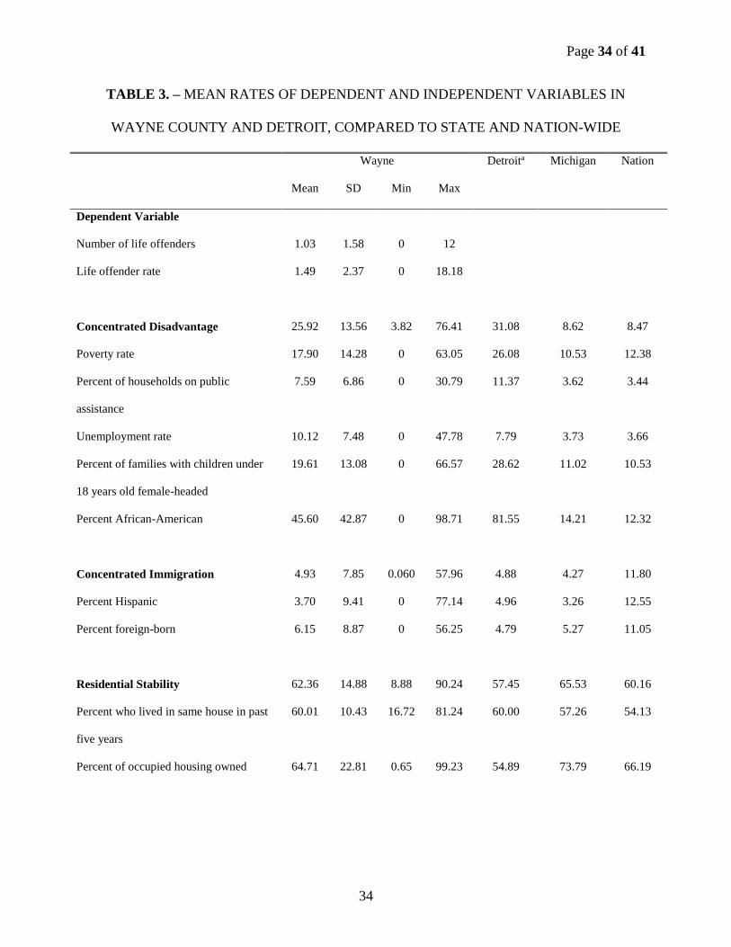
Table 3 gives the descriptive statistics for the dependent and independent variables. To

provide a comparative view, rates and values nation-wide, in the state of Michigan, and in

Detroit are also reported. Economic disadvantage in Wayne County is evident – it has higher

rates of concentrated disadvantage as well as lower rates of concentrated wealth than the rest of

Michigan and the United States. Compared to Wayne County, there is greater economic inequity

in Detroit, where both CD and CA rates are higher. For the other two social disorganization

scales, residential stability in Wayne County is similar to the rest of the U.S. and concentrated

immigration is lower. Despite the Latino enclave in Southwest of Detroit, the numbers are still

not as high as other cities such as those in Texas and Florida.

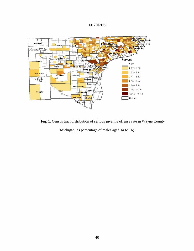
Fig. 1 maps the life offender rate into eight classes (separated by ArcGis according to

natural breaks in the data), from white representing tracts with no life offenders to the darkest

brown representing the five tracts with the highest life offender rates. The map depicts visually

the concentration of higher offense rates in Detroit (outlined in bold) and sparseness elsewhere.

All five of the highest offense tracts and most of the tracts in the next two high offense classes

are in Detroit.

Table 4 shows the strong correlations between the Census factors and life offender rates,

Table 4A for the structural scales and Table 4B for the individual variables. Table 4A shows that

all the correlations are high in the expected direction except for concentrated immigration.

Looking at the two variables in CI in Table 4B, one sees that while the proportion of Hispanic

residents is not significantly related to offender rates, the percentage of foreign born residents

significantly decreases the rate of life offenders instead of increasing it as predicted by theory. In

of 41

16

addition, the correlation between having stayed in the same house in the last five years and life

offending is small and insignificant. The correlations of these three variables with the other

independent variables are also low. Hence, even without multivariate analysis, the story of

immigration and home ownership in Detroit is diverging from the social disorganization story.

MULTIVARIATE ANALYSIS

How do the above relationships hold up when other factors are held constant? Table 5

presents negative binomial regression coefficient estimates of census scales in column (1) and

individual census variables in columns (2) and (3). Let us first discuss the expected results in

column (1). As predicted by theory, tracts with more life offenders are economically more

disadvantaged, less affluent, and more unequal. In particular, the positive coefficient of the

interaction term shows that when a larger percentage of the community is disadvantaged, greater

concentration of affluence increases offending (therefore inequality increases), and vice versa.

The loss of social control through immigration and residential instability, however, is

unsupported in this Wayne County data. While greater concentration of Latinos and immigrants

did correlate positively with more serious crime by youth, the association was statistically

insignificant. Outright contradicting theory is residential stability. After controlling for other

structural characteristics in the neighborhood, greater stability correlated with more serious

offending. Column (2) with individual variables shows that it is the home ownership rate that

caused this result. By social disorganization, more home owners should provide greater stability

and social control against crime than when residents are renters. However, after controlling for

other socioeconomic conditions, a higher percentage of home owners induced higher offending

of 41

17

rates instead. That is, if two neighborhoods have the same SES, family structures and racial

composition, the neighborhood with a larger proportion of homeowners have more offenders.

Why is this so? Examination of the tracts with the highest rental rates revealed that a few

were in the neighborhoods near to Wayne State University and the commercial downtown of

Detroit. These might have been neighborhoods where students and young professionals lived. In

contrast, similar SES and ethnic neighborhoods with higher home-ownership rates might have

comprised of residents who had owned homes which they were not able to leave.

Besides the significance of home ownership, column (3) shows that the percent of

population who are on PA, percent of single female headship, percent of African-Americans, and

percent of Hispanics continue to be significantly associated with more offenders. The results are

consistent with Wilson (1987, 1996)’s intertwining stories between social isolation and economic

disadvantage.

The race and ethnic interaction terms show that racial/ethnic heteregoneity are important

to the crime story in Wayne as well. As suggested at the onset that Hispanic immigrants might

inject control rather than disorganization, the negative coefficient from interacting percent

African-American with percent Hispanic shows that neighborhoods with greater proportions of

African-Americans have fewer serious youth offenders when there are more Hispanic residents,

and vice versa. This protective effect of Hispanic residents is played out even more by

comparing the results of the interaction terms in columns (2) and (3). In Column (2), where there

is no interaction of White and Hispanic, interacting percent African-American and White gives a

significant effect as predicted by social disorganization, that heterogeneity between these two

races induces crime. However, when White-Hispanic heterogeneity is added in column (3),

of 41

18

Black-White heterogeneity is no longer significant. However, the protective effect of Hispanics

in neighborhoods with higher proportions of African-Americans and Hispanics sustains.

If one returns to the variance inflation factors in table 4b, one may be tempted to discount

the results from the specification with individual variables as multicollinear. However, the

multivariate results signal no such problem. When there is multi-collinearity, the coefficient

estimates of the collinear variable will be sharply reduced. In this case, the two culprits – poverty

and female headship – continue to be large and statistically significant. With strong theoretical

reasons for the inclusion of these two variables, they were left in the model.

IMPLICATIONS FOR DEALING WITH JUVENILE CRIME

This analysis focused on a location that possesses problems and issues that are particular

to its historical development. The results therefore have limited generalizability. Methodological

limitations also constrain interpretations of results. First, Duncan and Raudenbush (1999)

suggests that neighborhood studies at times overestimate neighborhood effects because they are

proxying for family factors and at times underestimate effects because census tracts and zip

codes define neighborhoods inappropriately. Both problems apply in this study because it uses

census tracts and does not possess family or individual levels variables. Second, because

individual and process variables are unavailable, the findings in this study cannot be interpreted

as causal. As a cross-sectional study, this study faces the classic problem of whether

neighborhoods are bad because bad households choose to live in them or whether family

outcomes become bad as a result of living in bad neighborhoods.

Nevertheless, the significance of factors such as concentrated disadvantage implies that

something in the youthful offender’s environment matters, whether it is at the neighborhood or

of 41

19

family level. In addition, whether it is the variable measured in this analysis or some unobserved

factor correlated to it, addressing youth crime warrants consideration of the significant variables

because of comorbidity in conditions. Although generalizability is limited, the study offers some

general lessons because the results here are consistent with what some other studies have found.

First, the findings on immigrants and residential stability are antithesis to social

disorganization theories, but consistent with other studies that take into account local conditions

(e.g. Nielsen et al., 2005; Martin, 2002). Even the findings of Sampson 1997 and Morenoff et al.

(2001) on Chicago found similar results, although they did not explain the results because their

focus was on collective efficacy. These results imply that migration patterns have changed in

modern U.S. cities, so that immigrant concentration may instead bring organization into

previously depressed communities. In the 1960s, home ownership may indeed indicate greater

stability and immigrant enclaves may indeed have lower bonds and control, but given the

economic deprivation of African-Americans since the 1970s, the tide has changed.

Second, the indices that yielded significant results were also the same as those in

Sampson et al. (1997) and Morenoff et al. (2001). In the two studies and in this study, the

economic variables were consistently significant - economic deprivation and when included,

economic affluence and inequality as well. Breaking the indices down into individual variables

also delineated the significance of disadvantage through high concentrations of black and single-

headed families. These results gel with the theoretical foundation of social disorganization.

One implication of the above results is that dealing with crime in cities like Detroit

requires decisive intervention in such issues as economic opportunities especially in poor

neighborhoods where blacks and single parents are prevalent. Several national development

programs already have sites in Wayne County. However, the effectiveness of these programs is

of 41

20

unclear. Take the example of three promising community building programs that are related to

youth offending.

The first is the Weed and Seed Strategy, a community-based approach sponsored by the

U.S. Department of Justice (DOJ). Led by the relevant U.S. Attorney’s Office, Weed and Seed

takes a comprehensive multi-agency approach to achieving four main roles: (1) law enforcement;

(2) community policing; (3) prevention, intervention, and treatment; and (4) neighborhood

restoration (Office of Justice Programs, 2008). Out of eleven Michigan sites listed on the

website, four are in Wayne County. However, none of the Wayne County sites were included in

any of the evaluation reports available in the Weed and Seed Data Center. Only one Michigan

site, Grand Rapids, was briefly mentioned in a meta-analysis in 2004 (Justice Research and

Statistics Association, 2004).

Another example is YouthBuild. It engages unemployed, low-income 16 to 24 year old

early school leavers to build affordable housing for homeless and low-income people while they

are studying in a YouthBuild alternative school (The Bridgespan Group, 2004). The YouthBuild

site in Detroit is called Detroit Young Builders (DYB) and started in 1996. Outcomes seem to

have been encouraging: in its ten years program cycle, it had enrolled 516 young people, 96

percent of whom completed the program and went on to apprenticeships, universities or jobs

averaging $8.50 per hour (Young Detroit Builders, 2008). However, when YouthBuild USA

piloted the Youth Offender Project in 2004, DYB was not one of the 30 sites selected. The

selection criteria had included: (1) site demonstrates successful outcomes and operates high-

quality programs and services; (2) site demonstrates effective partnership building, is supported

within the community, and is viewed as a community resource; (3) site demonstrates an ability to

of 41

21

reach the intended target population; and leadership; (4) site demonstrates the ability to mobilize

resources and staff, and can quickly and effectively operationalize grant components.

At the state level, the Michigan Prisoner Re-entry Initiative (MPRI) is an ambitious

program started in 2005. With the tagline “creating safer neighborhoods and better citizens”, the

mission of the MPRI is to “reduce crime by implementing a seamless plan of services and

supervision developed with each offender—delivered through state and local collaboration—

from the time of their entry to prison through their transition, reintegration, and aftercare in the

community”. By 2007, MPRI had 15 sites and by 2008, every county had a site. With 34 percent

of prisoners returning to Wayne, out of which 80 percent returned to Detroit (Michigan Prisoners

Reentry Initiative, 2007), the Wayne County site is a key site which was part of the first phase.

So far, results of MPRI are positive as matched recidivism rates with pre-MPRI cohorts have

been lower. However, the April 2008 report warned that “adequate follow-up time must pass

before reliable recidivism outcomes can be established, since relatively few offenders are

returned to prison during the first several months following release” (Michigan Prisoners Reentry

Initiative, 2008, p.21). In addition, these aggregate results do not tell us whether MPRI has been

effective with the specific population in this study, i.e. the juveniles who were transferred to the

adult system.

Unfortunately, going by recent statistics, the above promising programs do not look so

effective anymore. In 2004, Detroit’s unemployment rate of 14 percent (Bureau of Labor

Statistics, 2004) and poverty rate of 33.6 percent (American Community Survey, 2004) were the

highest among the 50 largest cities in America, and the violent crime rate was 17 per 1,000

inhabitants, the fourth highest in the nation (Federal Bureau of Investigation, n.d.-b). Compare

these to the statistics given at the beginning of the article, and it is clear that conditions have

of 41

22

worsened since 2000. Why? Perhaps larger macroeconomic forces such as the sub-prime crisis

overwhelmed well-intentioned efforts. But since macroeconomic trends impact the whole

nation, why has Detroit’s ranking worsened relative to other cities in the country?

One proposition is the double distress of a city in dire straits combined with problems of

politics and leadership in this declining city. The controversial office of Detroit’s Mayor, Kwame

Kilpatrick, is one case in point. Since becoming Mayor, he has been entangled in scandal. The

scandals included racking up luxurious expenses such as spa treatments and champagnes during

times when the city was dismissing police officers to cut a $250 million budget deficit and the

most recent charges of lying under oath. Although he has been credited for bringing in large

investments such as casinos and hosting of Superbowl 2006, the criticism is that these are wooed

with tax breaks which do not benefit local small businesses or residents (Dalmia, 2008, p. A7;

Fears, 2008, p.A03).

However, fixing the leadership problem is only part of the solution. Managing a city that

is “dying a slow death” (Reese, 2006) is immensely challenging. Comparing Detroit to New

Orleans, Reese (2006) suggested applying responses to sudden natural disasters to cities

experiencing slow death: media attention; a sense of urgency coupled with long range vision;

coordinated federal, state, and foundation assistance; an emphasis on community hope; and a

focus on the public sector, public investment, public infrastructure, and public pride. Her views

are compelling and the findings in this article illustrate the urgency of dealing decisively with the

problems in Wayne County that intertwine crime with economic distress.

We need more crime ecological research in Detroit to better understand criminogenic

socio-economic conditions AND processes. This study had only census variables. Better data

from administrative sources and evaluations of existing programs are needed. Of the three

of 41

23

examples cited in this study, the MPRI research is the only one documented to be rigorous and

multi-year. For other programs, research does not seem to have kept pace with programs and the

programs may be inadequate. If ethnicity and family structure are important domains to crime

disadvantage, criminal justice requires better understanding of the extent to which crime control

initiatives tackle these issues.

Even without further research, though, some conclusions can be made that compel action.

The findings in this study are not surprising. People know that poor neighborhoods are homes to

more criminals. However, it is striking that this study finds significant results that are consistent

with Sampson et al. (1997) and Morenoff et al. (2001) when the study joins two very different

data sources and analyzes a different population of offenders (juvenile versus adult and all types

of serious offenses versus homicide) in a different city (Detroit versus Chicago). It seems that

juvenile serious offending relates to neighborhood characteristics in a similar way that adult

crime does. In fact, delinquency theory tells us that juvenile offending should be even more

influenced by environmental factors than adult crime.

The stark contrasts in neighborhoods and the high correlation of economic disadvantage

and inequality to juvenile crime documented in this study demands a response. The findings

justify the need for more comprehensive neighborhood solutions as integral to criminal justice,

from crime prevention to sentencing to re-entry. As Reese (2006) suggested, Wayne County

needs the same sense of urgency as when responding to natural disasters. It needs co-ordinated

efforts from the highest federal dollars to local government, community partners and private

enterprises. These are needed to restore hope and pride to a city in shambles.

of 41

24

ACKNOWLEDGEMENTS

This research was funded by the National University of Singapore Academic Research Fund (R-

134-000-056-112/133) and the Kellogg Foundation. The author thanks the Michigan Department

of Community Justice and the Wayne County Prosecutor’s Office for the provision of data.

Grateful thanks also to Rosemary Sarri, Sheldon Danziger, and Jeffrey Shook for comments at

various stages of the research; and Rebecca Tan and Helen Sim for research assistance.

of 41

25

NOTES

1 Facility addresses were investigated from two directions. First, repeated addresses were checked for addresses of

facilities. This identified four facilities, one of which is Wayne County Juvenile Detention Center (WCJDC) in the

excluded census tract 5172. The other three are out-county. This does not affect the sample in the sense that no in-

county data is lost. However, some of the cases which the data base gives a facility rather than family address may

have family origins in Wayne County. This means that the sample is missing some information. Second, the

addresses in the data base were compared against a directory of facilities and service providers with residential

programs. Only one case with a facility/provider address was found besides WCJDC. This case was left in the

sample.

of 41

26

REFERENCES

American Community Survey. (2004). Counties within United States – R1791. Percent of people

below poverty level. Retrieved March 27, 2009, from

http://factfinder.census.gov/servlet/GRTTable?_bm=y&-_box_head_nbr=R1701&-

ds_name=ACS_2004_EST_G00_&-_lang=en&-format=US-31&-CONTEXT=grt

Bergmann, L. (2008). Getting ghost: Two young lives and the struggle for the soul of Detroit.

New York: The New Press.

Block, R. (1977). Violent crime: Environment, interaction, and death. Lexinton, Mass: Lexinton

Books.

Brooks-Gunn, J., Duncan, G. J., Kato, P., & Sealand, N. (1993). Do neighborhood influence

child and adolescent behavior? American Journal of Sociology, 99(1), 353-395. doi:

10.1086/230268

Bureau of Labor Statistics. (2004). Unemployment rates for 50 largest cities (based on census

2000 population). Retrieved June 23, 2008, from http://www.bls.gov/lau/lacilg04.htm

Center for Urban Studies. (2008). The Hispanic population of southeast Michigan:

Characteristics and economic contributions. United States: Wayne State University.

Retrieved March 25, 2009, from

http://www.cus.wayne.edu/content/publications/hispaniccontributionstosem.pdf

Center for Urban Studies. (2001 May). International and domestic migration to metropolitan

areas in the United States, 1990-1999. Working Paper Series, No. 2. United States: Wayne

State University. Retrieved March 25, 2009, from

http://www.cus.wayne.edu/content/publications/eth_res_ser1.pdf

http://factfinder.census.gov/servlet/GRTTable?_bm=y&-_box_head_nbr=R1701&-ds_name=ACS_2004_EST_G00_&-_lang=en&-format=US-31&-CONTEXT=grt

http://factfinder.census.gov/servlet/GRTTable?_bm=y&-_box_head_nbr=R1701&-ds_name=ACS_2004_EST_G00_&-_lang=en&-format=US-31&-CONTEXT=grt

http://www.bls.gov/lau/lacilg04.htm

http://www.cus.wayne.edu/content/publications/hispaniccontributionstosem.pdf

http://www.cus.wayne.edu/content/publications/eth_res_ser1.pdf

of 41

27

Center for Urban Studies, & Skillman Center for Children. (2004). Detroit metropolitan census

2000 fact sheet series volume 4, issue 1: Latino children and families in the tri-county area.

United States: Wayne State University. Retrieved March 25, 2009, from

http://www.cus.wayne.edu/content/publications/latinocensusfactsheet.pdf

Coleman, J. S. (1988). Social capital in the creation of human capital. American Journal of

Sociology, 94(S1), S95-S120. doi:10.1086/228943

Coleman, J. S. (1990). Foundations of social theory. Cambridge, Mass: Belknap Press of

Harvard University Press.

Curtis, L. A. (1974). Criminal violence: National patterns and behavior. Lexington, MA:

Lexinton, Mass.

Dalmia, S. (2008, April 26). Cross country: Detroit's scandal is about more than sex. The Wall

Street Journal, pp. A7.

Duncan, G. J., & Raudenbush, S. W. (1999). Neighborhoods and adolescent development: How

can we determine the links? In A. Booth, & A. C. Crouter (Eds.), Does it take a village?

Community effects on children, adolescents, and families (pp. 106-135). New Jersey:

Lawrence Erlbaum Associates.

Farley, R., Danziger, S., & Holzer, H. J. (2000). Detroit divided. New York: Russell Sage

Foundation.

Fears, D. (2008, March 17). Yet more trouble for Detroit mayor; Kilpatrick defends use of racial

slur in his recent state of the city speech. The Washington Post, p. A03.

Federal Bureau of Investigation. (n.d.-a) Crime in the United States - 2000. Retrieved March 27,

2009, from http://www.fbi.gov/ucr/00cius.htm

http://www.cus.wayne.edu/content/publications/latinocensusfactsheet.pdf

http://www.fbi.gov/ucr/00cius.htm

of 41

28

Federal Bureau of Investigation. (n.d.-b) Crime in the United States 2004. Retrieved March 27,

2009, from http://www.fbi.gov/ucr/cius_04/

Gottfredson, D. C., McNeil III, R. J., & Gottfredson, G. D. (1991). Social area influences on

delinquency: A multilevel analysis. Journal of Research in Crime and Delinquency, 28(2),

197-226. doi:10.1177/0022427891028002005

Gyimah-Brempong, K. (2001). Alcohol availability and crime: Evidence from census tract data.

Southern Economic Journal, 68(1), 2-21.

Hipp, J. R. (2007). Income inequality, race and place: Does the distribution of race and class

within neighborhoods affect crime rates? Criminology, 45(3), 665-698. doi: 10.1111/j.1745-

9125.2007.00088.x

Justice Research and Statistics Association. (2004). Weed and seed local evaluation meta

analysis. Washington DC: Justice Research and Statistics Association. Retrieved March 25,

2009, from http://www.weedandseed.info/docs/studies_other/jrsa-meta-analysis.pdf

Kubrin, C. E., & Steward, E. A. (2006). Predicting who reoffends: The neglected role of

neighborhood context in recidivism studies. Criminology, 44(1), 165-197. doi:

10.1111/j.1745-9125.2006.00046.x

Land, K. C., & Deane, G. (1992). On the large-sample estimation of regression models with

spatial- or network-effects terms: A two-stage least squares approach. In P. Marsden (Ed.),

(pp. 221-248). San Fransico: Jossey-Bass.

Lee, M. T., & Martinez Jr., R. (2002). Social disorganization revisited: Mapping the recent

immigration and black homicide relationship in northern Miami. Sociological Focus, 35,

363-380.

http://www.fbi.gov/ucr/cius_04/

of 41

29

Martin, D. (2002). Spatial patterns in residential burglary: Assessing the effect of neighbourhood

social capital. Journal of Contemporary Criminal Justice, 18(2), 132-146. doi:

10.1177/1043986202018002002

Massey, D. S. (2001). The prodigal paradigm returns: Ecology comes back to sociology. In A.

Booth, & A. C. Crouter (Eds.), Community effects on children, adolescents, and families

(pp. 41-48). Mahwah, NJ: Lawrence Erlbaum Associates.

Michigan Prisoner Reentry Initiative. (2007). Michigan prisoner reentry initiative: Quarterly

status report. Retrieved March 25, 2009, from

http://www.michigan.gov/documents/corrections/MPRI_Quarterly_Status_Report_April_20

07_2nd_193517_7.pdf

Michigan Prisoner Reentry Initiative. (2008). Michigan prisoner reentry initiative: Quarterly

status report. Retrieved March 25, 2009, from http://www.michpri.com/uploads/Reports/04-

16-08_MPRI_Quarterly_Statue_Report__Addendum_231669_7.pdf

Miethe, T. D., & McDowall, D. (1993). Contextual effects in models of criminal victimization.

Social Forces, 71, 741-759.

Morenoff, J. D., Sampson, R. J., & Raudenbush, S. W. (2001). Neighborhood inequality,

collective efficacy, and the spatial dynamics of urban violence. Criminology, 39(3), 517-

560. doi: 10.1111/j.1745-9125.2001.tb00932.x

Nielsen, A. L., Martinez Jr., R., & Rosenfield, R. (2005). Firearm use, injury, and lethality in

assaultive violence: An examination of ethnic differences. Homicide Studies, 9(2), 83-108.

doi:10.1177/1088767904274160

http://www.michigan.gov/documents/corrections/MPRI_Quarterly_Status_Report_April_2007_2nd_193517_7.pdf

http://www.michigan.gov/documents/corrections/MPRI_Quarterly_Status_Report_April_2007_2nd_193517_7.pdf

http://www.michpri.com/uploads/Reports/04-16-08_MPRI_Quarterly_Statue_Report__Addendum_231669_7.pdf

http://www.michpri.com/uploads/Reports/04-16-08_MPRI_Quarterly_Statue_Report__Addendum_231669_7.pdf

of 41

30

Office of Justice Programs. (2008). Weed & seed – community capacity development office

(CCDO). Retrieved 23 June, 2008, from http://www.ojp.usdoj.gov/ccdo/ws/welcome.html

Ratcliff, J. H. (2004). Geocoding crime and a first estimate of a minimum acceptable hit rate.

International Journal of Geographical Information Science, 18(1), 61-72. doi:

10.1080/13658810310001596076

Reese, L. A. (2006). Economic versus natural disasters: If Detroit had a hurricane… Economic

Development Quarterly, 20(3), 219-231. doi: 10.1177/0891242406289344

Reiss, A. J., & Roth, J. A. (Eds.). (1993). Understanding and preventing violence. vol. 1.

Washington, D. C.: National Academy Press.

Sampson, R. J. (1999). How do communities undergird or undermine human development?

relevant contexts and social mechanisms. In A. Booth, & A. C. Crouter (Eds.), Does it take

a village? Community effects on children, adolescents, and families (pp. 3-30). New Jersey:

Lawrence Erlbaum Associates.

Sampson, R. J., Morenoff, J. D., & Earls, F. (1999). Beyond social capital: Spatial dynamics of

collective efficacy for children. American Sociological Review, 64(5), 633-660.

Sampson, R. J., Raudenbush, S. W., & Earls, F. (1997). Neighborhoods and violent crime: A

multilevel study of collective efficacy. Science, 277(15), 918-924. doi:

10.1126/science.277.5328.918.

Sampson, R. J., & Wilson, W. J. (1995). Towards a theory of race, crime, and urban inequality.

In J. Hagan, & R. D. Peterson (Eds.), Crime and inequality (pp. 126-137). Stanford, Calif:

Stanford University Press.

http://www.ojp.usdoj.gov/ccdo/ws/welcome.html

of 41

31

Shaw, C. R., & McKay, H. D. (1942). Juvenile delinquency in urban areas. Chicago: University

of Chicago Press.

Shook, J. J. (2004). Treating juveniles as adults: A case study of decision making and case

processing. Unpublished doctoral thesis, University of Michigan.

Smith, W. R., Frazee, S. G., & Davison, E. L. (2000). Furthering the integration of routine

activity and social disorganization theories: Small units of analysis and the study of street

robbery as a diffusion process. Criminology, 38(2), 489-524. doi: 10.1111/j.1745-

9125.2000.tb00897.x

The Bridgespan Group. (2004). YouthBuild USA: Achieving significant scale while guiding a

national movement. The Bridgespan Group, Inc.: Somerville, MA.

U.S. Census Bureau. (2008). United States Census 2000. Retrieved March 25, 2009, from

http://www.census.gov/main/www/cen2000.html

Wilson, W. J. (1987). The truly disadvantaged: The inner city, the underclass, and public policy.

Chicago: The University of Chicago Press.

Wilson, W. J. (1996). When work disappears: The world of the new urban poor. United States of

America: Vintage Books.

Young Detroit Builders. (2008). Young Detroit builders. Retrieved June 23, 2008, from

http://www.youngdetroitbuilders.org/

http://www.census.gov/main/www/cen2000.html

http://www.youngdetroitbuilders.org/

of 41

32

TABLES

TABLE 1. – ONE VARIMAX ROTATED FACTOR LOADINGS OF CENSUS VARIABLES

INTO FOUR FACTORS

Variable Factor 1 Factor 2 Factor 3 Factor 4

Poverty rate 0.91 -0.27 0.13 -0.16

Percent of households on public assistance 0.89 -0.25 0.010 -0.049

Unemployment rate 0.85 -0.25 -0.084 -0.026

Percent of families with children under 18 years old female-

headed

0.83 -0.30 -0.29 -0.24

Percent African-American 0.78 -0.13 -0.45 0.020

Percent Hispanic -0.0048 -0.21 0.56 -0.070

Percent foreign born -0.12 0.011 0.74 -0.21

Percent who lived in same house in past five years -0.12 -0.0023 -0.23 0.69

Percent of occupied housing owned -0.66 0.13 -0.061 0.59

Percent of family incomes greater than $75,000 -0.59 0.69 -0.023 0.18

Percent of professional or managerial occupations -0.42 0.78 -0.020 -0.046

of 41

33

TABLE 2. – FREQUENCIES OF SERIOUS JUVENILE OFFENDERS

BY AGE AND YEAR (N=761)

Frequency

Age 14 148

15 256

16 357

Year 1998 204

1999 190

2000 142

2001 122

2001 103

of 41

34

TABLE 3. – MEAN RATES OF DEPENDENT AND INDEPENDENT VARIABLES IN

WAYNE COUNTY AND DETROIT, COMPARED TO STATE AND NATION-WIDE

Wayne Detroita Michigan Nation

Mean SD Min Max

Dependent Variable

Number of life offenders 1.03 1.58 0 12

Life offender rate 1.49 2.37 0 18.18

Concentrated Disadvantage 25.92 13.56 3.82 76.41 31.08 8.62 8.47

Poverty rate 17.90 14.28 0 63.05 26.08 10.53 12.38

Percent of households on public

assistance

7.59 6.86 0 30.79 11.37 3.62 3.44

Unemployment rate 10.12 7.48 0 47.78 7.79 3.73 3.66

Percent of families with children under

18 years old female-headed

19.61 13.08 0 66.57 28.62 11.02 10.53

Percent African-American 45.60 42.87 0 98.71 81.55 14.21 12.32

Concentrated Immigration 4.93 7.85 0.060 57.96 4.88 4.27 11.80

Percent Hispanic 3.70 9.41 0 77.14 4.96 3.26 12.55

Percent foreign-born 6.15 8.87 0 56.25 4.79 5.27 11.05

Residential Stability 62.36 14.88 8.88 90.24 57.45 65.53 60.16

Percent who lived in same house in past

five years

60.01 10.43 16.72 81.24 60.00 57.26 54.13

Percent of occupied housing owned 64.71 22.81 0.65 99.23 54.89 73.79 66.19

of 41

35

TABLE 3 (CONT’D). – MEAN RATES OF DEPENDENT AND INDEPENDENT

VARIABLES IN WAYNE COUNTY AND DETROIT, COMPARED TO STATE AND

NATION-WIDE

Wayne Detroita Michigan Nation

Mean SD Min Max

Concentrated Affluence

25.62

14.83

4.23

77.48

18.90

31.01

30.69

Percent of family incomes greater than

$75,000

25.32 17.52 8.88 90.24 16.17 30.54 27.73

Percent of professional or managerial

occupations

25.92 13.56 3.82 76.41 21.63 31.48 33.65

Control and interaction variables

Percent white 46.83 40.43 0.25 97.37 12.26 80.15 75.14

Population densityb 33.96 13.03 5.06 99.52

Number of males aged 14 to 16 74.42 36.09 4 228

aRates in Detroit significantly different from non-Detroit rates at 5 percent except concentrated immigration.

bPopulation density by land area in kilometers X 10,000

TABLE 4A – CORRELATION MATRIX OF PERCENT OF LIFE OFFENDERS AND CENSUS SCALES

1 2 3 4 5 VIFc

1. Life offender rate 1.00

2. Concentrated Disadvantage 0.51* 1.00 3.10

3. Concentrated Immigration -0.047 -0.24* 1.00 1.39

4. Residential Stability -0.24* -0.53* -0.18* 1.00 1.92

5. Concentrated Affluence -0.40* -0.65* 0.084* 0.44* 1.00 1.95

cThe Variance Inflation Factor (VIF) is a measure of multicollinearity. Generally, a VIF of 10 and above is considered too large.

37

TABLE 4B – CORRELATION MATRIX OF PERCENT OF LIFE OFFENDERS AND CENSUS VARIABLES 1 2 3 4 5 6 7 8 9 10 11 12 13 VIF

1. Life offender rate 1.00

2. Poverty rate 0.48* 1.00 10.34

3. Percent of households on

public assistance

0.53* 0.89* 1.00 6.37

4. Unemployment rate 0.47* 0.85* 0.82* 1.00 4.64

5. Percent families with

children under 18 years

old female-headed

0.48* 0.84* 0.84* 0.79* 1.00 9.78

6. Percent African-American 0.45* 0.68* 0.72* 0.71* 0.86* 1.00 5.09

7. Percent White -0.47* -0.75* -0.76* -0.74* -0.85* -0.97* 1.00

8. Percent Hispanic 0.046 0.13* 0.042 0.0045 -0.068 -0.23* 0.014 1.00 1.47

9. Percent foreign-born -0.13* 0.023 -0.079 -0.19* -0.29* -0.42* 0.25* 0.47* 1.00 2.28

10. Percent who lived in same

house in past five years

-0.012 -0.24* -0.15* -0.10* -0.22* 0.062 0.014 -0.16* -0.31* 1.00 2.05

11. Percent of occupied

housing owned

-0.31* -0.75* -0.63* -0.60* -0.71* -0.51* 0.58* -0.11* -0.080* 0.54* 1.00 3.97

12. Percent of family incomes

greater than $75,000

-0.40* -0.75* -0.69* -0.67* -0.73* -0.56* 0.63* -0.15* 0.0032 0.13* 0.60* 1.00 5.67

13. Percent of professional or

managerial occupations

-0.35* -0.58* -0.58* -0.55* -0.57* -0.40* 0.45* -0.19* 0.082* 0.027 0.34* 0.82* 1.00 4.06

38

TABLE 5. – NEGATIVE BINOMIAL REGRESSION COEFFICIENTS OF CENSUS

FACTORS ON JUVENILE SERIOUS OFFENDINGd

(1) (2) (3)

Concentrated Disadvantage (CD)

1.103

(0.139)**

Concentrated Immigration (CI) 0.073

(0.083)

Residential Stability (RS) 0.836

(0.269)**

Concentrated Affluence (CA) -0.980

(0.216)**

CD X CA 0.547

(0.214)*

Poverty rate 4.660 4.091

(3.400) (3.460)

Percent of households on public assistance 0.402 0.399

(0.169)* (0.169)*

Unemployment rate 0.193 0.203

(0.181) (0.181)

Percent of families with children under 18 0.657 0.661

years old female-headed (0.301)* (0.301)*

Percent African-American 0.412 0.464

(0.139)** (0.152)**

Percent Hispanic 0.166 0.177

(0.085) (0.086)*

Percent foreign born -0.006 0.001

(0.090) (0.090)

Percent who lived in same house in past

0.266

0.275 five years (0.413) (0.413)

Percent of occupied housing owned 0.617 0.616

(0.181)** (0.180)**

39

TABLE 5 (CONT’D). – NEGATIVE BINOMIAL REGRESSION COEFFICIENTS OF

CENSUS FACTORS ON JUVENILE SERIOUS OFFENDINGd

(1) (2) (3)

Percent of family incomes greater than $75,000 -0.318 -0.290

(0.194) (0.196)

Percent of professional or managerial occupations -0.095 -0.083

(0.167) (0.167)

Poor X Rich 0.212 0.185

(0.153) (0.156)

African American X White 0.100 0.073

(0.047)* (0.056)

African American X Hispanic -0.164 -0.150

(0.071)* (0.073)*

White X Hispanic 0.079

(0.093)

Population densitye 0.002 0.003 0.003

(0.005) (0.005) (0.005)

Number of males aged 14 to 16 0.009 0.008 0.008

(0.001)** (0.001)** (0.001)**

Constant -4.832 -19.793 -18.808

(1.165)** (8.065)* (8.126)*

Observations 605 605 605

-659.37 -643.10 -642.74 dStandard errors in parentheses, * significant at 5%; ** significant at 1%

ePopulation density by land area in kilometers X 10,000

40

FIGURES

Fig. 1. Census tract distribution of serious juvenile offense rate in Wayne County

Michigan (as percentage of males aged 14 to 16)

Where Juvenile Serious Offenders Live: A Neighborhood ...WHERE JUVENILE SERIOUS OFFENDERS LIVE: A...

Documents

Transcript of Where Juvenile Serious Offenders Live: A Neighborhood ...WHERE JUVENILE SERIOUS OFFENDERS LIVE: A...