“When it rains, it pours”: fiscal policy, credit constraints

and business cycles in emerging and developed economies ∗

Krastina Dzhambova †

October 2017

The most recent version can be found here

Abstract

Fiscal pro-cyclicality, meaning co-movement between government expenditure and macroe-

conomic fundamentals, is an important feature of business cycle dynamics for emerging and

poor economies. I estimate a panel SVAR to investigate if fiscal policy leads to heightened

volatility, reinforcing the cycle in emerging economies. The analysis also sheds light on the

role of external financial constraints in shaping fiscal policy. My findings suggest that the

response of emerging governments to output fluctuations is similar to that of developed gov-

ernments. However, emerging governments curtail spending in response to increases in the

sovereign borrowing rate, which forces their consumption expenditure to act more pro cycli-

cally. While I find evidence of higher fiscal discretion in emerging economies, the government

consumption multiplier is substantially smaller for this group. For this reason, fiscal policy

is responsible for a lower share of business cycle volatility in emerging economies than in

developed ones.

JEL classification: F41, G15, E62, H50.

Keywords : fiscal procyclicality, country risk premium, international business cycles, general gov-

ernment consumption expenditure

∗I am grateful to my advisors Peter Ireland, Fabio Ghironi and Christopher Baum for their valuable comments,

suggestions and encouragement.†Department of Economics, Boston College;

email: dzhambov@bc.edu; website: https://sites.google.com/site/krastinadzhambovabc/

1

1 Introduction

The empirical international finance literature has long emphasized excess volatility that business

cycles in emerging and poor economies exhibit. Relative to the developed world, these economies

have higher volatility of all aggregate demand components as well as more frequent and deeper

crises (Uribe and Schmitt-Grohe (2017)). Another strand of research sheds light on the tendency

of fiscal policy to be pro-cyclical in these economies. This paper explores the relationship be-

tween these two stylized facts. In particular, I study the question of business cycle volatility in

emerging economies through the lens of the “when it rains, it pours” phenomenon. Dubbed so by

Kaminsky et al. (2004), this is a situation in which recessions are reinforced by capital outflows

coupled with a pro-cyclical policy stance.1 Kaminsky et al. (2004) among others2 document that

while in general net capital flows are pro-cyclical across poor, emerging and developed economies,

the cyclicality of (fiscal) policy variables differs between the developing and developed group. In

particular, developing economies exhibit fiscal policy pro-cyclicality which is difficult to justify as

a policy prescription.3

This paper aims to uncover the reasons for and the consequences of fiscal pro-cyclicality. On one

hand, policymakers themselves could be the source of volatility through discretionary interventions.

On the other hand, it is reasonable to expect that policymakers in the developing and emerging

world face constraints which impede their role as insurers against macroeconomic volatility. Inter-

national borrowing costs have been emphasized as important drivers of business cycle fluctuations

in emerging economies. Finally, even if policy itself does not cause or contribute to macroeco-

nomic volatility, the same policy design will lead to different outcomes both in terms of policy and

private sector variables when the underlying macro shocks are different. In short we want to ask

whether the macroeconomic woes of these economies are self-induced or the result of more volatile

underlying shocks, coupled with potentially tighter constraints faced by these governments. If the

latter is true, we also want to know if the excess volatility originates at home through a more

volatile process for GDP, for example, or abroad through asset price shocks. In this context, I try

to assess what fraction of business cycle fluctuations can be attributed to sovereign rate shocks

1Kaminsky et al. (2004) explore both fiscal and monetary policy cyclicality among developing, emerging anddeveloped countries. This paper focuses on fiscal policy although as a natural continuation the interaction betweenfiscal and monetary policy as well as exchange rate policy is to be considered

2see Talvi and Vegh (2005), Gavin and Perotti (1997)3The term pro-cyclicality itself requires a careful definition. As emphasized by Kaminsky et al. (2004), perhaps

the most convenient measure to use to identify potential differences in the conduct of fiscal policy is governmentexpenditure as opposed to revenue and primary balance in levels and as a share of GDP. In terms of governmentexpenditure, fiscal pro cyclicality is defined as a positive co-movement between government expenditure and GDP.Other researchers have defined pro-cyclicality in terms of taxes: the government raises tax rates in recessions. Directevidence on tax rates is sparse so researchers have used government revenue statistics and anecdotal evidence tomake the case for fiscal pro-cyclicality in developing economies. Finally, primary balance statistics highlight thatfiscal outcomes are different for the developing world but they are hard to use to disentangle the causes behindthose results.

2

versus policy shocks.

In order to understand the causes behind the “when it rains, it pours” phenomenon, I estimate a

panel SVAR on a large group of developed and emerging economies. I focus on government con-

sumption expenditure as the fiscal policy variable with the largest cross-country data availability.

The analysis has to overcome the issues of endogeneity between 1) fiscal policy and fundamentals

2) international borrowing cost and fundamentals and 3) international borrowing cost and fiscal

policy. A number of papers have emphasized the feedback between fundamentals and borrowing

costs for emerging economies.4 Fiscal policy variables also both respond to and influence the state

of the economy. Finally, fluctuations in the price of externally traded sovereign debt put a con-

straint on policymakers’ ability to use fiscal policy for stabilization. There are several pass-through

channels for a sovereign interest rate shock to influence the cycle. First, if government spending

contracts in response to increases in the borrowing cost, there is a standard multiplier effect which

decreases output and affects investment and consumption contingent on wealth effects and the

strength of Ricardian equivalence. Second, the government might shift part of the debt burden do-

mestically thus crowding out investment and consumption. Finally, rising sovereign rates can affect

the private economy if interest rate shocks pass through to households and firms via the banking

sector.5 In order to shed light on these questions, the analysis needs to isolate orthogonal shocks to

policy variables, fundamentals and international borrowing costs. Although fiscal pro-cyclicality is

normally discussed in the context of emerging and developing economies, the European debt crisis

made the interaction between fiscal policy, government finances and the real economy a relevant

issue for developed economies as well. In contrast to much of the literature, this paper studies

both developed and emerging economies. I compare the behavior and the effect of government

consumption spending across the two groups. I also characterize the effect of sovereign rate shocks

on government consumption spending as well as their direct and indirect effect on private sector

variables.

My identification strategy combines the Blanchard and Perotti (2002) SVAR approach to iden-

tify fiscal shocks and Uribe and Yue (2006) identification of external borrowing cost shocks. The

methodology proposed by Blanchard and Perotti (2002) uses institutional knowledge to put con-

straints on the impact matrix in a VAR analysis. In particular, the identification scheme assumes

that discretionary fiscal responses take place with one period delay. The use of quarterly data

is essential for implementing this identification strategy. For the purpose of identifying external

borrowing costs, Uribe and Yue (2006) propose an ordering of the impact matrix which leads to

impulse responses consistent with the standard small open economy real business cycle model (SOE

4see Uribe and Yue (2006), Mendoza and Yue (2012)5see De Marco (forthcoming) for quantifying government debt distress pass-through to firm loans in the context

of developed economies and Arteta and Hale (2008) in the context of emerging economies

3

RBC). The current study offers a unified framework for considering the interactions among funda-

mentals, fiscal policy shocks and external financial conditions.6Apart from the variables commonly

included in the analysis, I also consider the interplay among the government response function, the

dependence of spreads on both aggregate conditions and the government policy stance. This ap-

proach allows me to retrieve estimates of the policy response function to output and international

borrowing costs as well as the coefficients on the government debt pricing function. I also trace

out the dynamic effect of orthogonal shocks to income, sovereign yields and government spending.

My findings suggest that government consumption, a category of government expenditure, is pro-

cyclical for both emerging and developed economies. The systematic response of both types of

economies to output fluctuations is virtually the same. Emerging economies are however more

sensitive for changes in international borrowing conditions. Higher output relaxes international

borrowing constraints. As a result, GDP shocks lead to an overall bigger increase in government

consumption in emerging economies. This finding suggests that as far as government consumption

is concerned, increases in this fiscal expenditure component during good times is not symptomatic

of political frictions. Instead the higher fiscal pro-cyclicality in emerging economies is the result

of these governments being more sensitive to international borrowing conditions. However, the

analysis reveals that discretionary interventions are much more common in the emerging world.

This raises concerns because a higher degree of policy discretion has been shown to have a negative

effect on long run growth and volatility.

I investigate the differential role of international financial conditions for policy and business cycle

outcomes of emerging and developed economies along two dimensions: shocks to the international

safe borrowing rate and shocks to the price of a country’s government debt on international mar-

kets. Fluctuations in the safe rate have a negligible impact on the business cycle and the fiscal

stance in either group of countries. Shocks to the government borrowing rate have different im-

plications for the developed versus the emerging group. An exogenous increase in the sovereign

rate is contractionary in both economies. In the emerging group these shocks are more important

for output fluctuations, while in the developed group they matter relatively more for investment

dynamics.

6Another strategy for identifying the effect of fiscal policy changes at business cycle frequency is the narrativeapproach advocated by Romer and Romer (2010) among others. The narrative approach uses information containedin government documents and announcements to identify periods of fiscal expansion or consolidation which areunrelated to the business cycle. The identification procedure which uses military build up in wartime to identifygovernment spending episodes unrelated to the business cycle is a special case of the narrative approach. Examplesof this approach used on U.S data include Barro (1981), Hall (1986), Hall (2009), Rotemberg and Woodford (1992),Barro and Redlick (2011). As military build-up episodes are not common during the same time as most detailedmacroeconomic data is available for the developing world, I adhere to the SVAR identification approach to estimatethe policy reaction function and the government spending multiplier.Sheremirov and Spirovska (2017) exploit anew military spending database to estimate multipliers for a large number of countries. Despite the difference inidentification, our estimates are in line.

4

My results also shed light on the efficacy of government consumption as a policy tool. The es-

timated long run multiplier effect of government consumption on output is less than 1 for both

country groups. However, the government consumption multiplier is twice as high for the developed

group, pointing to a substantially impaired ability of government consumption shocks to influence

the economy in emerging countries. My results also imply that government consumption expen-

diture shocks account for a smaller fraction of business cycle fluctuations in emerging economies.

Despite the high volatility of these shocks in the emerging world, they claim a smaller share of

the volatility of macroeconomic variables because of the smaller multiplier. Shocks to government

consumption also account for a smaller share of the sovereign rate fluctuations emphasizing the

fact that these governments have been more careful about international borrowing conditions. The

paper provides estimates of the officially reported

In this paper I also document differences in fiscal statistics and their relationship with the cycle

among a large group of poor, emerging and rich countries. I highlight that in terms of correlations

to the cycle, government expenditure is pro-cyclical in poor and emerging economies as stressed in

the literature. It is important however to look at individual components of government expenditure

as this is a fairly large category which encompasses all of government expense as well as investment

(Table 1). When focusing specifically on government consumption of goods and services, I find

that this fiscal expenditure category is pro-cyclical across the board with group differences stem-

ming from higher volatility of government consumption rather than cyclicality. The SVAR analysis

currently focuses on government consumption expenditure. As confirmed by summary statistics

the distinction among different components of government expenditure is important. Government

consumption expenditure is only one component of automatic stabilization. Therefore, lack of

other automatic stabilizers (e.g. social transfers (unemployment benefits, safety-net program),

retirement and health benefits, progressive taxes and proportional taxes) in emerging economies

might be behind the difference in government expenditure cyclicality.7

Recent policy challenges in developed economies, such as monetary authorities grappling with the

zero lower bound on short run nominal rates and fiscal stimulus packages emerging as an important

policy tool, have sparked renewed academic interest in the topic of fiscal policy and business

cycles. In the next section I discuss how this paper relates to several branches of the literature:

discretionary fiscal policy, political frictions and macroeconomic outcomes, cost of borrowing and

business cycles, external shocks and macroeconomic volatility. Section 3 describes the sources and

construction of the dataset used in the paper. Section 4 describes the behavior of key fiscal variables

7McKay and Reis (2016) provide model-based estimates of the ability of US built-in stabilizers to decrease con-sumption and output volatility. They find that the social insurance role (the tax-and-transfer system) of stabilizersis more important than the New Keynesian demand stabilization channel.

5

across poor, emerging and developed economies. Section 5 discusses the SVAR methodology while

section 6 discusses the empirical results. Section 7 and section 8 focus on the variance and the

variance decomposition of estimated shocks. Section 9 presents robustness checks which extend the

analysis to subsets of the data or employ an alternative estimation strategy. Section 10 concludes.

2 Links to the Literature

The vast majority of the studies on discretionary fiscal policy are conducted on US and to a

lesser extent OECD data. Using US data and a VAR approach, Blanchard and Perotti (2002)

estimate a government spending multiplier around 1; Fatas and Mihov (2001) obtain estimates

well above 1 while Mountford and Uhlig (2009) find large debt financed tax multipliers but low

government spending multipliers for the US. Based on the narrative approach, Ramey (2011) finds

a wide range of multipliers for the US including estimates above 1 depending on the time period.8,9

There is a nascent literature on quantifying the effects of fiscal policy outside developed economies.

The influential paper by Ilzetzki et al. (2013) sets the beginning of an exciting strand of research

by offering the first cross-country comparison of government consumption multipliers that spans

poor, emerging and developed country groups. Jawadi et al. (2016) focuses explicitly on emerging

economies and estimates a PVAR on the BRICs. Jawadi et al. (2016) find strong New Keynesian

effects of government purchase shocks; they also find evidence of monetary accommodation in these

economies raising concerns about monetary authority independence for this group. 10 The present

8Although the government spending multiplier emerges as a convenient statistic to describe the efficacy ofdiscretionary changes in fiscal policy, there are three important channels government spending and governmentrevenue shocks influence economic activity: 1) the effect of fiscal policy on the composition of GDP (privateconsumption and investment), 2) the effect on asset prices such as stocks and housing markets 3) the effect onthe external sector. The question of whether private consumption increases in response to a positive governmentspending shock has been investigated at length by both the theoretical and the empirical literature. From atheoretical standpoint Gali et al. (2007) shows in the context of a New Keynesian model that breaking the Ricardianequivalence is essential for getting consumption to respond positively to an expansion in government spending. Galiet al. (2007) among many others consider the presence of hand-to-mouth consumers to decrease the negative wealtheffect of present or future increase in taxes to finance the fiscal consumption which is responsible for the fall inconsumption in the standard New Keynesian and neoclassical model. Offsetting the fall in consumption also leadsto a higher output multiplier potentially above 1.

9Non-linearities in the effect of fiscal policy have been emphasized by the literature. Perotti (1999) finds thatgovernment spending decreases private consumption in debt-stressed economies. There is some evidence in theliterature that composition of government expenditure matters for the value of the multipliers. Abiad et al. (2016)public investment increases output and employment in both the short and long run in advanced economies especiallyduring periods of slack; the effect on investment has the opposite sign depending on the state of the economy withan expansionary effect during periods of low output.

10Another point of interest concerning the international dimensions of fiscal policy relates to the Mertens andRavn (2011) focus on the real exchange depreciation puzzle in response to government expenditure shock presentin developed countries’ data. While output and consumption rise and the trade balance deteriorates in response toa government expenditure shock in these economies, the real exchange rate is empirically found to depreciate. Theauthors rationalize the depreciation through a model featuring deep habits in both private and public consumptionand the decrease in mark-ups due to the increase in government consumption demand.

6

study contributes to this strand of literature by comparing the design of fiscal policy across country

groups in addition to the more commonly discussed fiscal multipliers. My particular focus is the

importance of external borrowing costs for shaping the conduct of fiscal policy. Having estimates

of the government response function, allows me to quantify the extent to which the response of

emerging governments to output fluctuations is different from that of developed. The comparison

is a test for the existence of political frictions in emerging economies relative to developed. In terms

of the government consumption multiplier, my results for the group of countries in my dataset are

in line with those in Ilzetzki et al. (2013), particularly in the sense that higher level of development

makes fiscal policy more effective.

One important question I set out to answer is whether observed differences in fiscal outcomes

between emerging and developed countries stems from political frictions or whether they can be

explained from a purely macroeconomic perspective. Woo (2009) and Ilzetzki (2011) motivate pro

cyclicality in government expenditure with political and social polarization. In these papers polit-

ical underrepresentation or institutional infighting about the types of public good to be provided

makes government expenditure more sensitive to revenue fluctuations. Frankel et al. (2012) relate

government expenditure pro cyclicality to lack of good institutions and find empirical evidence

that improving the soundness of institutions helps the pro cyclicality issue. Alesina and Tabellini

(2008) propose a model of political agency problem to explain why more corrupt governments

fail to insure efficiently private consumption. In their model public outlays rise in response to an

expansionary income shock. These expansions in government spending are due to governments

extracting higher rents when times are good. Overall models based on political frictions predict

that government expenditures are more sensitive to output and revenue fluctuations relative to

the efficient benchmark. The SVAR analysis presented in this paper suggests that emerging gov-

ernments are indeed more sensitive to fundamentals, but in the sense of international borrowing

constraints and not shocks to domestic income. Therefore, external borrowing costs seem to be

more important in shaping fiscal policy design in emerging economies than political frictions.

International credit conditions have been emphasized in the literature on emerging economies

business cycles as an important source of uncertainty. Models which allow credit frictions to af-

fect directly not only consumption smoothing but also labor demand have been shown to deliver

properties consistent with stylized facts.1112Given this evidence, it comes as no surprise that in-

ternational credit markets and / or financial frictions have been among the suspected reasons for

11see for instance Neumeyer and Perri (2005) and Mendoza and Yue (2012)12Uribe and Yue (2006) and Akinci (2013) present a PVAR analysis of a group of emerging economies and find

that the estimated impulse responses of fundamentals are consistent with the theoretical impulse responses arisingfrom a model with a working capital constraint. Uribe and Yue (2006) find that international capital markets affectemerging economies through risk premium shocks and to much lesser extent through shocks to the global risk-freerate. Akinci (2013) shows that shocks to international risk appetites are another source of variation which can causebusiness cycle slumps in the emerging world.

7

fiscal pro cyclicality in emerging markets. Riascos and Vegh (2003) and Cuadra et al. (2010) pro-

pose models to justify why taxes on consumption in the former case and labor income taxes in

the latter case might behave pro cyclically when the international asset markets are incomplete or

when premiums on government debt are determined a la Arellano (2008) respectively. In terms

of pro-cyclicality on the expenditure side, Mendoza and Oviedo (2006) show that a government

which faces a more volatile revenue stream sets lower debt limits for itself. Bi (2012) offers an

alternative explanation; it is the volatility of government expenditure that leads to lower debt

limits.13 The current paper strives to offer a unified approach for measuring interactions between

internal fundamentals, external shocks and government expenditure.

This paper also contributes to the literature on measuring the role of external shocks for business

cycle fluctuation in emerging and developing economies.14 Raddatz (2007) estimates the effect of

external shocks emanating from commodity price fluctuations, natural disasters and the interna-

tional economy on low income and poor economies and finds that external shocks are responsible

for only a small share of output fluctuation in this group of economies. My conclusions are similar

in regard to international sovereign rate shocks- I find that these shocks are more contractionary in

emerging economies and account for a bigger share of output fluctuations. Nonetheless the overall

share of business cycle fluctuations they account for is small.

3 Data

As the identification strategy for government consumption shocks hinges on the use of quarterly

data, I compile a data set of quarterly output, investment, net trade and government consumption

expenditure for a panel of emerging and developed economies. I use government consumption

because among the components of total government expenditure it has the best cross-country

availability at quarterly frequency. The data sources are IMF IFS and Eurostat. All series are

deflated using the series specific price index when available or the Producer Price Index. Data is

deseasoned and linearly detrended. 15

To measure the external borrowing cost faced by the sovereign, I use the J.P.Morgan Emerging

Market Bond Index Plus (EMBI+)16 for emerging economies and the J.P.Morgan Government

13in the model in Bi (2012) government expenditure alternates between a stationary and a non stationary processwith an exogenous probability.

14Using a BVAR analysisErten (2012) finds that external demand shocks accounted for roughly 50% of thevariation in GDP growth for a sample of Latin American economies during the European debt crisis.

15similar results obtain if I detrend the data quadratically16According to the J.P.Morgan documentation provided by Datastream the EMBI+ contains only bonds or loans

issued by sovereign entities form index-eligible countries.

8

Bond Index (GBI) series for developed economies. Both indices are constructed by J.P.Morgan as

a representative investment benchmark for a country’s internationally traded sovereign debt and

thus are a good proxy for how international investors price sovereign debt. Both indices cover debt

instruments denominated in US dollars and span all available maturities. To proxy for the safe

rate, I follow the rest of the literature and use the 10-year US treasury yield. In order to obtain

measures of real return on government debt, I adjust both the sovereign yields and the safe rate by

US expected inflation, which is proxied by a four-quarter rolling average of the US CPI. I obtain

the quarterly GBI and EMBI+ as well as the 10-year US treasury series from Thomson Reuters

Datastream.

The inclusion of countries in my dataset is guided by the coverage of the two sovereign bond

indices- EMBI+ and GBI. The inclusion of a country in either index implies that it is viewed

by international financial markets as belonging to either group. Therefore I can use the time

series for these countries to measure how international investors price sovereign debt and to quan-

tify group difference in that respect. Following the groups delineated by the two sovereign bond

indices, I included the following countries in my analysis: 1) developed economies : Australia, Aus-

tria, Belgium, Canada, Denmark, Finland, France, Germany, Greece, HK, Ireland, Italy, Japan,

Netherlands, Portugal, Spain, Sweden and the UK; 2) emerging economies : Argentina, Brazil,

Bulgaria, Colombia, Ecuador, Mexico, Peru, Philippines, Russia, South Africa, Turkey, Ukraine.17

As a robustness check I also report results excluding the distressed European economies from the

sample. The time series length for each panel is determined by the coverage of the sovereign bond

indices. The beginning of the indices also roughly coincides with the beginning of the time series

on government consumption for emerging economies. The resulting time series length is Q1 1994

to Q4 2014. My panel comprises a total of 30 countries and 84 quarters.

The annual data on fiscal variables is drawn from the IMF WEO. It covers the time period from

1980 to 2014 for 168 countries. The advantage of the annual data is the wider country and fiscal

variable coverage relative to what is available at the quarterly frequency. I use this data to revisit

the problem of fiscal pro-cyclicality and to verify if the pattern of greater procyclicality is present

beyond the late 1990s as emphasized by the previous literature.

4 Pro-cyclicality at Annual Frequency

As a first stab at the data, I take a look at the annual series to determine if the pro cyclicality

of government expenditure and government consumption for emerging and developing economies

characterizes the data once the sample is extended with recent data. I find that government

17I drop Croatia (15 quarters), Egypt (25 quarters), Hungary (14 quarters), Indonesia (32 quarters), Poland (51quarters), Malaysia (12 quarters) as they were included in the EMBI+ for less than 15 years

9

expenditure does behave differently between rich economies and the rest. Figure 1 shows the

contemporaneous correlation between the cyclical component of real GDP and real government

expenditure. I calculate the group specific correlation using both data series in levels and in first

difference to alleviate concerns about stationarity. I also summarize the group specific distribu-

tion in terms of a simple as well as a population weighted mean. Additionally, I provide a check

by netting out interest payments from total expenditure. Because we should anticipate that the

composition and the yield curve of sovereign debt differs among the three country groups, interest

payments might be confounding the degree of pro cyclicality. 18 Across the board the correlation

is different from 0 with the exception of the case of rich economies in levels. Overall there is strong

evidence that government expenditure is pro-cyclical for the emerging and the poor group relative

to the rich group. As the t tests suggest the correlation is indistinguishable between emerging and

poor but the rich group is significantly different from the rest in terms of the cyclicality of govern-

ment expenditure. The exception is the case for the population weighted correlation. In this case

the poor group shows the most counter-cyclical stance. The population weights emphasize India

and China for which the correlation is negative. As Figure 3 shows pro-cyclicality is decreasing

in country size for poor and emerging, but particularly so for poor. I report population weighted

correlations excluding India and China. In this case the pro-cyclicality pattern emerges again.

Figure 2 reports the volatilities among the 3 groups. As the literature has emphasized, the cycle

is at least 50% more volatile for poor and emerging economies than for industrial economies. The

table also reports the volatility of government expenditure relative to output. Across the three

groups government expenditure is more volatile than output. While in terms of output volatil-

ity poor and emerging are indistinguishable from one another and more volatile than industrial

economies, in terms of government expenditure volatility, the emerging group looks similar to the

developed groups in terms of both magnitude of the statistic and the t test. Government expen-

diture is significantly more volatile in emerging economies than developed only for the series in

difference and population weighted mean. To summarize, government expenditure for emerging

economies is similar to the poor group in terms of cyclicality and similar to the developed group

in terms of volatility.

Another relevant statistic to look at is the amplitude of government expenditure growth defined

as the difference between expenditure growth during booms relative to expenditure growth during

recessions. As consistent business cycle dating is not available across a large number of economies,

I take an approach exploited in the literature and report the average growth when real GDP growth

is above median versus below median. Figure 4 reports the results. The amplitude of government

expenditure for poor and emerging is in stark contrast to industrial. According to this statistic

18the contemporaneous correlation increases from expenditure to net expenditure for emerging and rich but norfor poor.

10

government expenditure is acyclical for industrial and strongly pro-cyclical for poor and emerging.

The table also reports amplitude for government revenue. The literature has suspected that the

revenue process for emerging and poor governments is more volatile and governments are more con-

strained in raising revenue. The amplitude statistic does show a modestly greater pro-cyclicality

of revenue for poor and emerging but the difference is not as stark as in the expenditure case.

Finally figure 5 reports the OLS estimates of the elasticity of government revenue and expenditure

to real GDP. The revenue elasticity of 1 for industrial is consistent with the literature. Govern-

ment revenue is more responsive to fluctuation in real output in the case of emerging and poor

economies. The pooled OLS estimate for the elasticity of expenditure to GDP uncovers again

evidence of greater pro-cyclicality of government expenditure.

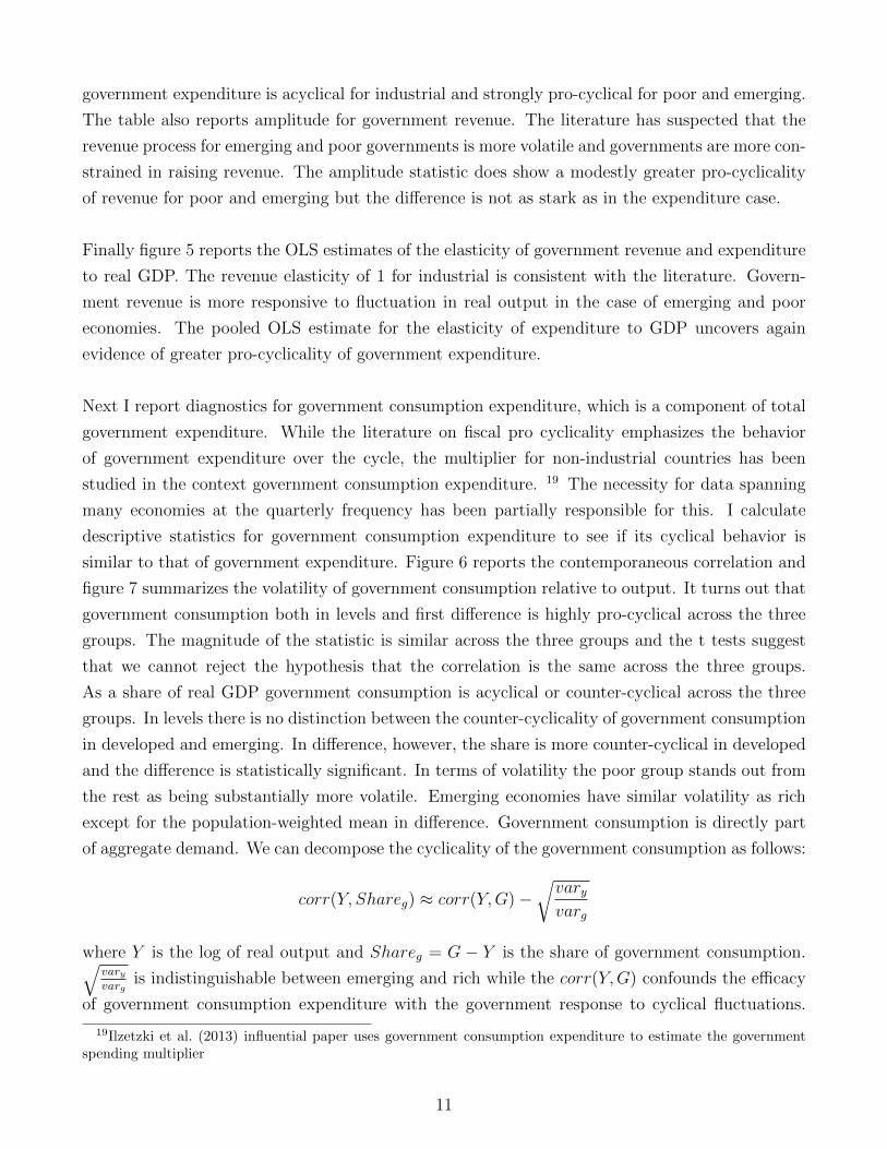
Next I report diagnostics for government consumption expenditure, which is a component of total

government expenditure. While the literature on fiscal pro cyclicality emphasizes the behavior

of government expenditure over the cycle, the multiplier for non-industrial countries has been

studied in the context government consumption expenditure. 19 The necessity for data spanning

many economies at the quarterly frequency has been partially responsible for this. I calculate

descriptive statistics for government consumption expenditure to see if its cyclical behavior is

similar to that of government expenditure. Figure 6 reports the contemporaneous correlation and

figure 7 summarizes the volatility of government consumption relative to output. It turns out that

government consumption both in levels and first difference is highly pro-cyclical across the three

groups. The magnitude of the statistic is similar across the three groups and the t tests suggest

that we cannot reject the hypothesis that the correlation is the same across the three groups.

As a share of real GDP government consumption is acyclical or counter-cyclical across the three

groups. In levels there is no distinction between the counter-cyclicality of government consumption

in developed and emerging. In difference, however, the share is more counter-cyclical in developed

and the difference is statistically significant. In terms of volatility the poor group stands out from

the rest as being substantially more volatile. Emerging economies have similar volatility as rich

except for the population-weighted mean in difference. Government consumption is directly part

of aggregate demand. We can decompose the cyclicality of the government consumption as follows:

corr(Y, Shareg) ≈ corr(Y,G)−√varyvarg

where Y is the log of real output and Shareg = G − Y is the share of government consumption.√varyvarg

is indistinguishable between emerging and rich while the corr(Y,G) confounds the efficacy

of government consumption expenditure with the government response to cyclical fluctuations.

19Ilzetzki et al. (2013) influential paper uses government consumption expenditure to estimate the governmentspending multiplier

11

As the SVAR analysis discussed in the subsequent sections shows the government response in

emerging economies is more pro-cyclical due to credit constraints while the efficacy of government

consumption is substantially lower for emerging economies.

In the previous sections I review evidence of whether fiscal pro cyclicality is still present in the

data. The behavior of pro cyclicality over time warrants attention because Frankel et al. (2012)

offers evidence that fiscal pro cyclicality (measured as the correlation between annual government

expenditure and the cyclical component of gdp) has decreased over time for some developing and

emerging economies. They relate this change to institutional improvement in this group of coun-

tries. Figure 8 plots the rolling window correlation between the cyclical component of GDP and

government expenditure for the three groups of countries. I report the correlation for a 5, 10 and

15 years horizon. While there is an improvement across the all groups over the 90s and early 2000s,

the correlation is U-shaped. In other words there is a reversal to pro-cyclicality towards the end of

the sample. Figure 9 repeats the same exercise for net government expenditure (excluding interest

expense). The same pattern emerges. This ensures me that the question of fiscal pro-cyclicality is

still empirically relevant.

Although the analysis does not include direct measures of capital flows, I look at the cyclical

behavior of the GBI and the EMBI Plus indices next. Figure 11 shows the empirical distribution

of sovereign rate on international financial markets adjusted for inflation. The left pane excludes

only realization during default while the right pane excludes defaulters in the sample altogether

(Argentina, Ecuador, Greece and Russia). On average emerging governments pay up to 4% higher

rates on international borrowing. The standard deviation of the pooled realized rates appears

similar, but this clearly driven by the exorbitant yields faced by Greece during the European bond

crisis. Excluding Greece as well as the other defaulters highlights the fact that the distribution for

emerging yields is also more spread out. Figure 12 reports the median rate for each country in the

sample. The fact that emerging governments pay a higher rate on external obligations emerges

again. Within the developed group, the GIIPS pay higher rates than the rest of the developed

economies. South Africa’s median rate on the other hand is comparable to developed economies’

rates. Towards the top of the two groups, we find governments that experienced default during

the sample years- Greece for developed and Argentina and Ecuador for emerging. I report median

rates to attenuate the effect of default episodes. Nonetheless the relative country order is barely

changed in terms of the average rate and maximum realized rate for each country (Figure 13).

Finally, Figure 14 reports the sovereign rates of the distressed European economies relative to

several GBI averages during the European debt crisis. Clearly Greece experienced an exorbitant

hike reflected in the Greek GBI index. Greece’s interest spike is followed by Portugal and Ireland’s

and to a lesser extent by Spain and Italy. The GBI average excluding the distress economies are

actually decreasing. As a robustness check (reported in a subsequent section), I discuss excluding

12

the GIIPS from the analysis.

5 Identification

The widely accepted identification outlined by Blanchard and Perotti (2002) uses institutional

knowledge. The paper as well as much of the subsequent literature constrain the government to

respond to macroeconomic fundamentals with at least a quarter delayed. In other words within

a period the government cannot respond to macroeconomic fundamentals. The assumption is

justified by pointing out institution delays in implementing fiscal changes. The delays are related

to both collecting data on the private sector as well as the legislating and executing fiscal reforms.

For this reason the use of quarterly data is essential. This identification can be recast as an A

model outlined in detail in Lutkepohl (2007). In particular I assume that the observed relationships

in the data can be modeled as a stationary VAR of order p:

yt = A1yt−1 + ....+ Apyt−p + ut

yt is a vector [gt gdpt it tbyt rust Rt

]gt is government consumption, gdpt is output, it is in investment, tbyt is trade balance relative

to GDP, rust is the world safe rate proxy and Rt is the sovereign interest rate. All variables are

expressed in real terms.

Further I assume that there is an A matrix such that:

Ayt = A∗1yt−1 + ...+ A∗pyt−p + et

where et is a vector of orthogonal structural shocks with a diagonal Σe covariance matrix. The

assumption implies the A-model formulation:

Aut = et

with AAi = A∗i . After imposing appropriate restrictions on A we can bring the following system

to the data:

yt = [I − A]︸ ︷︷ ︸Aestimate

yt + A∗1yt−1 + ...+ A∗pyt−p + et

13

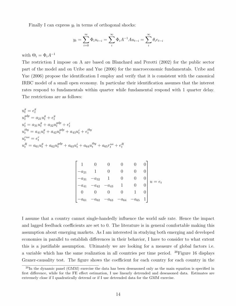
Finally I can express yt in terms of orthogonal shocks:

yt =∞∑i=0

Φiut−i =∞∑i

ΦiA−1Aut−i =

∞∑i

θiet−i

with Θi = ΦiA−1

The restriction I impose on A are based on Blanchard and Perotti (2002) for the public sector

part of the model and on Uribe and Yue (2006) for the macroeconomic fundamentals. Uribe and

Yue (2006) propose the identification I employ and verify that it is consistent with the canonical

IRBC model of a small open economy. In particular their identification assumes that the interest

rates respond to fundamentals within quarter while fundamental respond with 1 quarter delay.

The restrictions are as follows:

ugt = egt

ugdpt = a21ugt + eyt

uit = a31ugt + a32u

gdpt + eit

utbyt = a41ugt + a42u

gdpt + a43u

it + etbyt

urust = ert

uRt = a61ugt + a62u

gdpt + a63u

it + a64u

tbyt + a65r

ust + eRt

1 0 0 0 0 0

−a21 1 0 0 0 0

−a31 −a32 1 0 0 0

−a41 −a42 −a43 1 0 0

0 0 0 0 1 0

−a61 −a62 −a63 −a64 −a65 1

u = et

I assume that a country cannot single-handedly influence the world safe rate. Hence the impact

and lagged feedback coefficients are set to 0. The literature is in general comfortable making this

assumption about emerging markets. As I am interested in studying both emerging and developed

economies in parallel to establish differences in their behavior, I have to consider to what extent

this is a justifiable assumption. Ultimately we are looking for a measure of global factors i.e.

a variable which has the same realization in all countries per time period. 20Figure 16 displays

Graner-causality test. The figure shows the coefficient for each country for each country in the

20In the dynamic panel (GMM) exercise the data has been deseasoned only as the main equation is specified infirst difference, while for the FE effect estimation, I use linearly detrended and deseasoned data. Estimates areextremely close if I quadratically detrend or if I use detrended data for the GMM exercise.

14

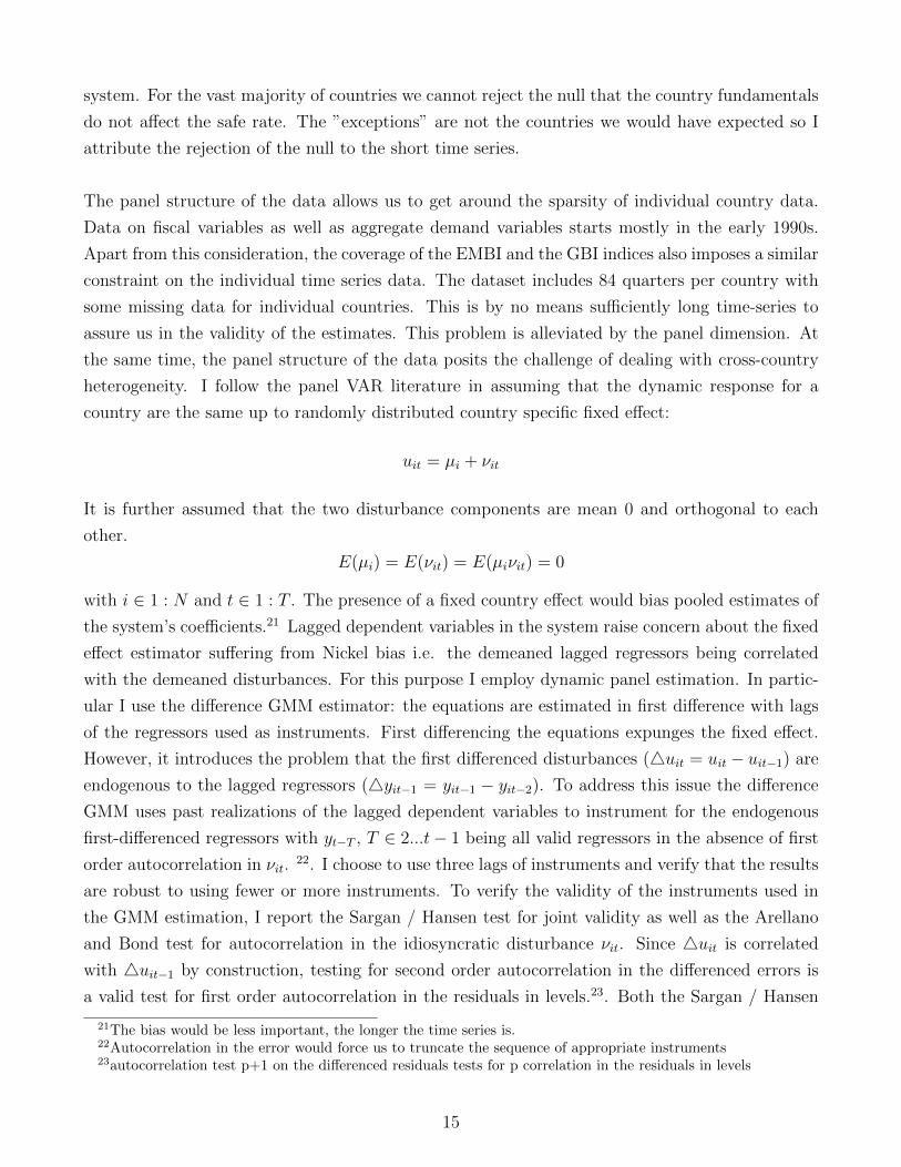
system. For the vast majority of countries we cannot reject the null that the country fundamentals

do not affect the safe rate. The ”exceptions” are not the countries we would have expected so I

attribute the rejection of the null to the short time series.

The panel structure of the data allows us to get around the sparsity of individual country data.

Data on fiscal variables as well as aggregate demand variables starts mostly in the early 1990s.

Apart from this consideration, the coverage of the EMBI and the GBI indices also imposes a similar

constraint on the individual time series data. The dataset includes 84 quarters per country with

some missing data for individual countries. This is by no means sufficiently long time-series to

assure us in the validity of the estimates. This problem is alleviated by the panel dimension. At

the same time, the panel structure of the data posits the challenge of dealing with cross-country

heterogeneity. I follow the panel VAR literature in assuming that the dynamic response for a

country are the same up to randomly distributed country specific fixed effect:

uit = µi + νit

It is further assumed that the two disturbance components are mean 0 and orthogonal to each

other.

E(µi) = E(νit) = E(µiνit) = 0

with i ∈ 1 : N and t ∈ 1 : T . The presence of a fixed country effect would bias pooled estimates of

the system’s coefficients.21 Lagged dependent variables in the system raise concern about the fixed

effect estimator suffering from Nickel bias i.e. the demeaned lagged regressors being correlated

with the demeaned disturbances. For this purpose I employ dynamic panel estimation. In partic-

ular I use the difference GMM estimator: the equations are estimated in first difference with lags

of the regressors used as instruments. First differencing the equations expunges the fixed effect.

However, it introduces the problem that the first differenced disturbances (4uit = uit − uit−1) are

endogenous to the lagged regressors (4yit−1 = yit−1 − yit−2). To address this issue the difference

GMM uses past realizations of the lagged dependent variables to instrument for the endogenous

first-differenced regressors with yt−T , T ∈ 2...t− 1 being all valid regressors in the absence of first

order autocorrelation in νit.22. I choose to use three lags of instruments and verify that the results

are robust to using fewer or more instruments. To verify the validity of the instruments used in

the GMM estimation, I report the Sargan / Hansen test for joint validity as well as the Arellano

and Bond test for autocorrelation in the idiosyncratic disturbance νit. Since 4uit is correlated

with 4uit−1 by construction, testing for second order autocorrelation in the differenced errors is

a valid test for first order autocorrelation in the residuals in levels.23. Both the Sargan / Hansen

21The bias would be less important, the longer the time series is.22Autocorrelation in the error would force us to truncate the sequence of appropriate instruments23autocorrelation test p+1 on the differenced residuals tests for p correlation in the residuals in levels

15

test and the Arellano and Bond test confirm that the matrices yt−p−i for i ∈ [1 : 3] are valid

instruments. Only for the investment equations we reject the null of no first order autocorrela-

tion. To alleviate this concern, I also report estimates of the third row of the Ai matrices using

alternative dynamic panel estimators.2425 While the dynamic panel estimators are less taxing

in terms of degrees of freedom loss due to deeper-lag instruments, the time series length (T =

82) in the data is perhaps sufficient to make the dynamic bias small and to justify the use of a

more straightforward estimation technique such as the fixed effect estimator. In turns out that in

this particular empirical specification the fixed effect estimates of the system lead to instability

issues. Empirically I demonstrate that the distressed European economies as a group are the po-

tential culprit. Excluding them indeed fixes the problem. I report fixed effect estimation for the

sample excluding this group (GIIPS: Greece, Italy, Ireland, Portugal, Spain) as a robustness check.

Finally in order to estimate differences in dynamic responses between developed and emerging

economies I modify the estimation to include an emerging-dummy interaction26:

al,ij = al,0(ij) + al,1(ij)× 1[EME]

al,ij is the ij-th element of Al for l ∈ [0..p] and EME selects the emerging economies in the sample.

The AIC criterion selects one lag as optimal (see Figure 37). The autoregressive coefficients

for the safe rate are estimated by OLS in first difference.

6 SVAR Analysis

Figure 31 and figure 32 show the GMM estimates of the system for both the developed and the

emerging group. Figure 33 explicitly focuses on the government response. Overall, the government

responds pro-cyclically to output for both groups. The point estimates suggest that worsening in-

ternational financial conditions decrease government consumption- increases in the safe rate as

well as the sovereign international borrowing rate lead to a decrease in government consumption

for both groups. Both the group by group estimates and the joint estimates suggest that emerging

economies are more mindful of international credit constraints and decrease government consump-

tion in response to an increase in the safe borrowing rate and their own sovereign borrowing

rate. Conversely, international credit constraints have a lower bite for governments in developed

economies vis-a-vis those in emerging economies. Moreover, the government response to output

24The Arellano Bond test statistic in constructed under the assumption of large N and small T as well asE(eitejt) = 0. Controlling for the safe rate helps with the latter assumption, but the relatively small N in theempirical sample (N = 30) might be problematic.

25For a comprehensive discussion of dynamic panel estimators and literature review see Roodman (2009)26this is equivalent to estimating the system separately for each group, but leads to a slight efficiency improvement

16

is similar for the two groups and statistically indistinguishable. This juxtaposition sheds light on

one of the main questions of the paper- whether emerging governments are more sensitive to the

cycle and whether they respond more procyclically to output fluctuations. Conditional on my

identification, it turns out this is not the case.

Figure 34 reports results for the government response function estimated using private GDP in-

stead. I confirm that emerging governments decrease consumption expenditure in response to

increases in the borrowing rate they face on international markets. This is still the main differ-

ence between the two government response functions. If anything, the coefficient on the interest

rate is even higher in magnitude when private gdp is used in the estimation. This is also the

case with FE estimates (figure 35).The FE estimation confirms that the main difference between

emerging and developed economies stems from their response to the sovereign rate. Differently

from GMM, the fixed effect estimation suggests that government consumption does not respond

to gdp fluctuations at all. The coefficient on real gdp is lower and imprecisely estimated. In the

next section I show that the bootstrapped impulse response still implies an increase in government

consumption following a positive output shock even in the FE estimation case. Finally, figure 36

shows another robustness check for the government response function. In particular, I report fixed

effect estimates for a country subset which excludes Greece, Portugal and Italy. Greece and Por-

tugal are the countries experiencing the largest increase in government yields relative to the rest

of several subsets of the GBI index family during the European debt crisis. I choose to report

this particular cut of the data because excluding all of the distressed European economies leads

to stability issues in the VAR analysis. I revisit this issues in the robustness section. I exclude

Greece, Portugal and Italy and re-estimate the system with FE. I also report results from GMM

estimation which excludes all distressed European economies (Greece, Portugal, Ireland, Italy and

Spain). This particular GMM estimation should be interpreted with care, because further de-

creasing the number of panels raises concerns. In the GMM case, the difference between the full

sample and the sub-sample for the developed group is that the coefficient on the lagged dependent

variable increases and there is no response of government consumption to fundamentals apart form

that to the safe rate. For the emerging group the GMM estimates on the subset suggest just the

opposite: government consumption is less persistent and more responsive to fundamentals relative

to emerging. The fixed effect estimates on the full sample and subsample are quite similar. In

both FE exercises governments do not respond to fundamentals apart from the sovereign rate.

Increases in the international sovereign rate are contractionary for both the full sample and the

subset albeit imprecisely estimated in the subsample case.

Returning to the rest of the variables in the model (figure 31 figure 32), we already see that the

efficacy of government consumption as a policy instrument is substantially lower as captured by the

impact coefficient on GDP. As anticipated an increase in government consumption is expansionary.

17

However, as the coefficient on the interaction (GC × I(Emerging)) suggests, the impact coefficient

for emerging economies is a third that for developed. The crowding-out of investment on the

other hand by government consumption is lower in emerging economies. The coefficient on L.GC

is practically off-set by the coefficient on L.GC×I(Emerging) for Investment. Although the cur-

rent analysis does not include measures of how the government finances government expenditure,

the lack of crowding out for investment is symptomatic of revenue financed increases in govern-

ment expenditure for emerging economies, which can be one factor behind the lower multiplier for

this group (I discuss the multiplier in the next section). The estimates suggest that government

consumption leads to a greater deterioration in the trade balance for developed economies which

is consistent with either a greater share of imported goods and services in the government con-

sumption basket or a stronger multiplier on private sector consumption. Finally, for either group

fluctuations in government consumption do not impact directly sovereign borrowing constraints.

As anticipated, investment is strongly pro-cyclical for both emerging and developed. The trade

balance is again as anticipated counter-cyclical due to the effect of investment as emphasized by

the IRBC. Sovereign credit constraints do not directly affect fundamentals except in the case of

investment for developed economies. On the other hand the sovereign rate shows a lot of persis-

tence for developed economies and less so for emerging. As a matter of fact I estimate a significant

feedback from output to the sovereign borrowing rate for emerging and not for developed. The

sovereign rate is less persistent in the case of emerging economies. To capture the rich dynamics

of the system I discuss the impulse response analysis in the next section.

6.1 Impulse Responses

6.1.1 Shocks to Government Consumption

Figure 17 reports the impulse response to a unitary orthogonal shock to government consumption

expenditure. Government consumption expenditure is expansionary for both emerging and rich

economies. For the rich group there is a greater evidence of investment crowding out during the

initial quarters for which the impulse response is statistically indistinguishable from 0. For sub-

sequent quarters developed economies investment is higher but the impulse responses for the two

groups are still statistically indistinguishable from each other. The effectiveness of government

consumption in stimulating output is ostensibly higher for the developed group. Government

consumption shocks cause a slight deterioration in the trade balance. Finally the response of

the interest rate is the mirror image for the two groups with borrowing conditions improving for

emerging economies in response to a government consumption shock. As we saw in the estimates

of the system the response of the borrowing rate is determined by the response of the rate to

output fluctuations rather than the directly through government consumption. Finally there is no

18

response of the world safe rate by construction. As the persistence of government consumption

differs between the 2 groups I calculate the multiplier next.

Figure 18 reports the government consumption multiplier. Following the literature, I define the

government consumption spending multiplier as:

impact multiplier =4X0

4G0

cumulative multiplier =

∑Tt=04Xt∑Tt=04Gt

Xt ∈[gt gdpt it tbyt rust Rt

]

Normally the literature reports the multiplier effect of government (consumption) expenditure

on GDP. To facilitate the comparison between the two groups, I report the multiplier effect of

shocks on all variables in the system. There is a striking difference between the multiplier effect

of government consumption on output in the two groups. In emerging economies government

consumption is substantially less effective in stimulating output; the impact multiplier is roughly

two times lower than the impact multiplier for developed economies. For both groups the multiplier

is less than 1, which is consistent with estimates of the multiplier in Ilzetzki et al. (2013). However,

differently from them I do not obtain negative multipliers. I do not find difference in the two

groups for the investment multiplier which is consistent with bigger crowding out for the developed

group. The deterioration in the trade balance is of similar magnitude for both groups. Finally,

as fundamentals improve, the sovereign borrowing rate also improves for emerging economies.

On impact, a unitary increase in government consumption leads to a 16 basis points decrease in

the rate. The cumulative multiplier effect is as high as 12%. In other words, a 10% increase in

government consumption decreases the sovereign borrowing rate by 1.23% for emerging economies

and while the same increase in government consumption would induce an increases in the rate

by 73 basis points for developed over the whole cycle. Figure 18 also reports the government

consumption multiplier on private gdp. The comparison between the two groups still holds with

the short-run multipliers being up to 3 times lower and the long run multiplier up to 2 times lower

for emerging economies. It should be noted that estimates deal with officially reported gdp. If we

had a measure of the informal sector or the shadow economy, estimates of the fiscal multiplier for

the informal sector would be also very informative.

19

6.1.2 Shocks to Output

Next I consider shocks to output. Figure 19 reports the response of the variables in the model

to a unitary shock to output. The empirical responses are consistent with the predictions of the

SOE IRBC model: investment responds more than one for one with output and the trade balance

is countercyclical. The impact response of investment in emerging economies is slightly higher.

However the investment response converges to being indistinguishable between emerging and rich as

the horizon increases. One of the key questions I am after is whether emerging governments respond

differently to output fluctuations; in particular whether government consumption expenditure re-

enforces the cycle. While the median response for emerging governments is higher, the response

of government consumption to output fluctuation is indistinguishable from the developed group’s.

This results suggests that emerging governments do not necessarily have a more pro-cyclical stance.

Instead as revealed by the response to interest rate shocks which is to be discussed next, government

consumption expenditure is more sensitive to sovereign interest rate shocks. The sovereign rate

responds to fundamentals in emerging economies while the response in developed is statistically

indistinguishable from 0. Figure 20 reports the multiplier effect of an output shock on the rest

of the model variables. The median multiplier effect of output on government consumption is

higher- between 4 to 24 percentage points, in emerging economies. Given that the coefficients

on the response function are the same, the higher multiplier is due to the fact that the increase

in output relaxes the borrowing constants for emerging governments. In other words, emerging

governments raise government consumption in response to a positive output shock because of

the relaxed international borrowing constraints. In particular in emerging economies the median

impact improvement in the government interest rate is 14 percentage points and the long run

improvement- 33 percentage points. For the developed group the improvement in the long run is

roughly 1 percentage point and is not statistically significant.

6.1.3 Shocks to the Sovereign Borrowing Rate

Figure 21 reports the impulse response of the model variables to a unitary shock in the sovereign

borrowing rate. The shock leads to a contraction in emerging economies albeit a milder one relative

to the estimates in Uribe and Yue (2006) and Akinci (2013). The developed group can weather

the shock without a significant decrease in the government consumption or output. However, for

the developed group, there is a substantial decrease in investment and an improvement in the

trade balance. To account for the difference in persistence of the shock propagation I recast the

impulse response in a multiplier form as shown in figure 22. The median multiplier for emerging

governments’ consumption to an interest rate shock is twice as high as that for developed. The

median response for output is twice as high. However, as noted before investment in developed

economies responds twice as strongly to an interest rate shock as investment in the emerging group.

20

6.1.4 Shocks to the Safe Rate

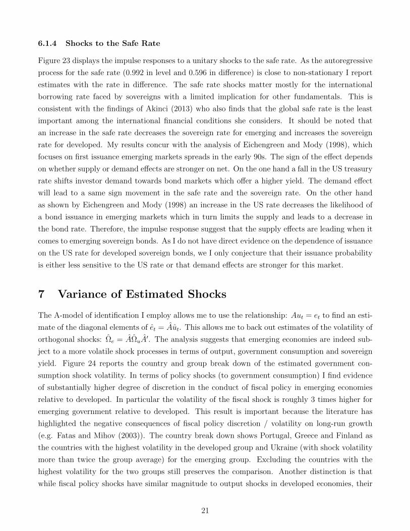
Figure 23 displays the impulse responses to a unitary shocks to the safe rate. As the autoregressive

process for the safe rate (0.992 in level and 0.596 in difference) is close to non-stationary I report

estimates with the rate in difference. The safe rate shocks matter mostly for the international

borrowing rate faced by sovereigns with a limited implication for other fundamentals. This is

consistent with the findings of Akinci (2013) who also finds that the global safe rate is the least

important among the international financial conditions she considers. It should be noted that

an increase in the safe rate decreases the sovereign rate for emerging and increases the sovereign

rate for developed. My results concur with the analysis of Eichengreen and Mody (1998), which

focuses on first issuance emerging markets spreads in the early 90s. The sign of the effect depends

on whether supply or demand effects are stronger on net. On the one hand a fall in the US treasury

rate shifts investor demand towards bond markets which offer a higher yield. The demand effect

will lead to a same sign movement in the safe rate and the sovereign rate. On the other hand

as shown by Eichengreen and Mody (1998) an increase in the US rate decreases the likelihood of

a bond issuance in emerging markets which in turn limits the supply and leads to a decrease in

the bond rate. Therefore, the impulse response suggest that the supply effects are leading when it

comes to emerging sovereign bonds. As I do not have direct evidence on the dependence of issuance

on the US rate for developed sovereign bonds, we I only conjecture that their issuance probability

is either less sensitive to the US rate or that demand effects are stronger for this market.

7 Variance of Estimated Shocks

The A-model of identification I employ allows me to use the relationship: Aut = et to find an esti-

mate of the diagonal elements of et = Aut. This allows me to back out estimates of the volatility of

orthogonal shocks: Ωe = AΩuA′. The analysis suggests that emerging economies are indeed sub-

ject to a more volatile shock processes in terms of output, government consumption and sovereign

yield. Figure 24 reports the country and group break down of the estimated government con-

sumption shock volatility. In terms of policy shocks (to government consumption) I find evidence

of substantially higher degree of discretion in the conduct of fiscal policy in emerging economies

relative to developed. In particular the volatility of the fiscal shock is roughly 3 times higher for

emerging government relative to developed. This result is important because the literature has

highlighted the negative consequences of fiscal policy discretion / volatility on long-run growth

(e.g. Fatas and Mihov (2003)). The country break down shows Portugal, Greece and Finland as

the countries with the highest volatility in the developed group and Ukraine (with shock volatility

more than twice the group average) for the emerging group. Excluding the countries with the

highest volatility for the two groups still preserves the comparison. Another distinction is that

while fiscal policy shocks have similar magnitude to output shocks in developed economies, their

21

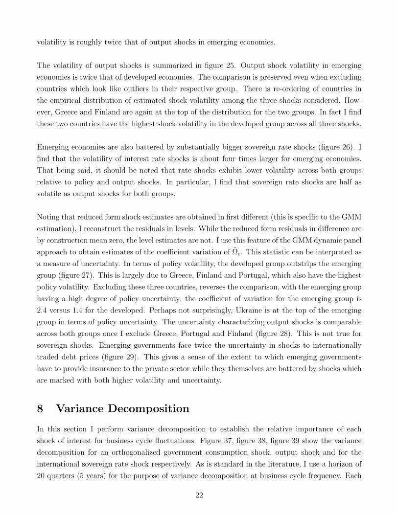
volatility is roughly twice that of output shocks in emerging economies.

The volatility of output shocks is summarized in figure 25. Output shock volatility in emerging

economies is twice that of developed economies. The comparison is preserved even when excluding

countries which look like outliers in their respective group. There is re-ordering of countries in

the empirical distribution of estimated shock volatility among the three shocks considered. How-

ever, Greece and Finland are again at the top of the distribution for the two groups. In fact I find

these two countries have the highest shock volatility in the developed group across all three shocks.

Emerging economies are also battered by substantially bigger sovereign rate shocks (figure 26). I

find that the volatility of interest rate shocks is about four times larger for emerging economies.

That being said, it should be noted that rate shocks exhibit lower volatility across both groups

relative to policy and output shocks. In particular, I find that sovereign rate shocks are half as

volatile as output shocks for both groups.

Noting that reduced form shock estimates are obtained in first different (this is specific to the GMM

estimation), I reconstruct the residuals in levels. While the reduced form residuals in difference are

by construction mean zero, the level estimates are not. I use this feature of the GMM dynamic panel

approach to obtain estimates of the coefficient variation of Ωe. This statistic can be interpreted as

a measure of uncertainty. In terms of policy volatility, the developed group outstrips the emerging

group (figure 27). This is largely due to Greece, Finland and Portugal, which also have the highest

policy volatility. Excluding these three countries, reverses the comparison, with the emerging group

having a high degree of policy uncertainty; the coefficient of variation for the emerging group is

2.4 versus 1.4 for the developed. Perhaps not surprisingly, Ukraine is at the top of the emerging

group in terms of policy uncertainty. The uncertainty characterizing output shocks is comparable

across both groups once I exclude Greece, Portugal and Finland (figure 28). This is not true for

sovereign shocks. Emerging governments face twice the uncertainty in shocks to internationally

traded debt prices (figure 29). This gives a sense of the extent to which emerging governments

have to provide insurance to the private sector while they themselves are battered by shocks which

are marked with both higher volatility and uncertainty.

8 Variance Decomposition

In this section I perform variance decomposition to establish the relative importance of each

shock of interest for business cycle fluctuations. Figure 37, figure 38, figure 39 show the variance

decomposition for an orthogonalized government consumption shock, output shock and for the

international sovereign rate shock respectively. As is standard in the literature, I use a horizon of

20 quarters (5 years) for the purpose of variance decomposition at business cycle frequency. Each

22

figure shows the share of the specified variable (government consumption, output and the rate) in

the h-step forward error variance decomposition for each variable in the system. The h-step ahead

forecast is given by:

yt − yt+h|t = ut+h + Φ1ut+h−1 + ...+ Φh−1ut+1

We can represent the forecast as a MA in terms of the structural errors:

yt − yt+h|t =h−1∑m=0

θmet+h−m

Then the FEV for a particular variable k in the system:

σ2k(h) =

∑κ

h−1∑m=0

θ2kκ,mΩe(κ, κ)

We can express FEV Dk,j: the share of variable j in the forecast error variance of variable k

setting j = κ:

Sk,j(h) =

∑h−1m=0 θ

2kj,mΩe(j, j)

σ2k(h)

The reported results for the government consumption shock suggest that innovations to govern-

ment consumption are responsible for 16% of output fluctuations in emerging economies and up

to 34% in developed. This result is rationalized by recalling that despite the high volatility of

government shocks, the efficacy of those shocks is roughly 50% lower in emerging economies. The

importance of government consumption shocks for investment is similar to their contribution to

output for the emerging group, while for the developed group government consumption shocks

contribute substantially more to output fluctuations than to investment fluctuations.

The contribution of sovereign rate fluctuations is arguably small for both country groups- 2% of

output in emerging and less than 1% in developed. My estimates are in the lower end of the

literature for emerging economies; Akinci (2013) for example estimates the contribution of inter-

national rate fluctuations to the variance decomposition of output in emerging economies to be

roughly 20%. My estimates are based on similar data. However, I explicitly account for the role of

government consumption, jointly estimate the model on both emerging and developed countries,

increase the time dimension by three years to include the taper tantrum and double the number

of panels. In contrast to the aforementioned paper I consider both dynamic panel estimates as

well as fixed effect estimation. It should be acknowledged that much in the spirit of the rest of

the literature, I find that sovereign rate shocks play a more important role for the emerging group

i.e. they account for twice the share of forecast error variance in emerging than in developed

economies. Another difference between the two groups is that in emerging economies interest rates

account for a smaller share of their own fluctuations. Thus the feedback between fluctuations in

23

fundamentals and international borrowing rates is stronger in emerging countries.

Of central interest to this paper is whether output fluctuations play a bigger role for government

consumption in the emerging group. It should be noted that both output and government con-

sumption shocks are more volatile in the emerging group as highlighted in the previous section. It

turns out that governments (in the sense of government consumption) are responsible for a similar

share of real GDP fluctuations across the two groups with developed countries actually surpassing

their emerging counterparts. The observation that government consumption is responsible for a

smaller share of output fluctuations in emerging economies while at the same time output being

responsible for a similar share of government consumption fluctuations leads me to conclude that

there is no dramatic difference in fiscal stabilization between the two groups as far as government

consumption is concerned. There is also a stark comparison between the role of output for interest

rate fluctuation in emerging economies. Output fluctuations are responsible for more than 20%

of the fluctuations in the price of international debt in emerging economies with this share being

substantially smaller in the developed group. Similarities emerge when looking at the share of

investment and trade balance fluctuations. Output fluctuations are responsible for a similar share

of investment and trade balance variance. For both groups output accounts for almost half of the

fluctuations in investment.

9 Robustness

In this section I explore to what extent results are sensitive to the choice of countries and to

including the European debt crisis in the sample. One concern would be related to the distressed

European economies and whether the identification imposing the same dynamic matrices across

both the core and the GIIPS is not too restrictive. Because decreasing the number of panels might

be problematic in the GMM cases, I choose to explore different country subsets in the context of

FE estimation. Before proceeding further I discuss some stability issues which emerge in the case

of Fixed Effect. Figure 44 shows the eigen values for selected dynamic matrices. The full sample

GMM is stable, but FE estimation for both the full sample and the sample excluding the GIIPS is

not. In both cases one of the eigen values is not strictly inside the unit circle. The issue pertains

specifically to the developed group; the eigen values for the emerging group are strictly inside

the unit circle for all cases. The issues for the developed group are due to the coefficient on the

sovereign rate. The fixed effect estimation implies an autoregressive coefficient for the developed

sovereign rate of 1.025 (standard error = 0.019) and 0.844 (standard error = 0.023) for emerging.

The autoregressive coefficient increases if the sovereign yield is specified in first difference; in par-

ticular for developed economies the coefficient increases to 1.763 (standard error = 0.173) while

for the emerging group the coefficient drops to 0.421 (standard error = 0.18). To shed more light

24

on the issue I estimate the bottom row of the dynamic matrices country by country. Figure 45

displays the autoregressive coefficient for each country. Excluding Greece, Italy and Portugal in-

duces stationarity as shown by the eigen values. 27

After excluding Greece, Portugal and Italy I re-do the impulse response analysis. Figure 41 reports

the result for a government consumption shock. Generally the two estimators agree on the role

and propagation of government consumption shocks. Overall the fixed effect estimation implies a

lower multiplier effect of a government consumption shock on output. However, the comparison in

terms of how effective policy shocks in emerging economies relative to developed are, still holds.

Government consumption is substantially more effective in developed economies. The sign of the

median investment, trade balance and sovereign rate impulse responses is unchanged relative to

the GMM estimation. However, the investment response is estimated with much wider confidence

bands for developed and is indistinguishable from 0 for emerging. The GMM estimation attributes

a bigger movement to investment, while the fixed effect estimation- to the trade balance. The fixed

effect estimation still implies an increase in international borrowing rates in response to a policy

shock for the developed group and just the opposite for the emerging group.

Figure 42 reports the impulse response of the system to output shocks for the FE effect estima-

tion case. This robustness check confirms that government consumption does not respond more

procyclically in the emerging group. It also confirms that output expansion decreases the interna-

tional borrowing rate for the emerging group. The biggest difference between the two estimators

stems from the behavior of the sovereign yield for developed. In contrast with the GMM estimates,

the FE impulse response is much more persistent and implies an increase in the sovereign rate in

response to an expansionary output shock.

Finally figure 43 provides estimates of the impulse response to a sovereign yield shock. The result

confirms that sovereign yield shocks are contractionary for emerging economies. The impulse

response for the developed group leads us to believe that the shock is contractionary for government

consumption and investment but expansionary for output. Because it would be difficult for most

open economy models to justify an expansion in output, I conclude that the GMM interest rate

impulse response is more plausible.

10 Conclusion

International borrowing costs and business cycles are interrelated in a complex way. The interna-

tional finance literature suggests that this relationship is stronger for emerging economies. Default

27Excluding Portugal is enough to induce stationarity, however results are very close to the case of excluding allthree distressed economies, which I report.

25

risk priced into their international borrowing costs makes these costs more tightly linked to fluctu-

ations in macroeconomic fundamentals. At the same time, emerging economies presumably have

less perfect shock absorption mechanisms relative to their developed counterparts. The contribu-

tion of this paper is two-fold; first, I evaluate the hypothesis that external borrowing costs are

more important drivers of business cycles in emerging economies by studying the question in a

panel of both emerging and developed economies. Second, I investigate the role that fiscal pol-

icy plays for the relationship between borrowing costs and business cycle fluctuations. Led by

identification demands on data availability, I focus on government consumption as a fiscal pol-

icy tool. Developed economies provide a benchmark against which the performance of emerging

sovereigns is studied. Relative to their developed counterparts, emerging economies’ governments

are more responsive to fluctuations in their sovereign yields and contract government consumption

in response to interest rate shocks. This creates a propagation mechanism allowing interest rate

increases to lead to business cycle contractions. As measured by the contraction in output, in-

terest rate shocks indeed lead to deeper contractions in emerging economies than in rich economies.

I also find that government consumption is a substantially weaker policy tool in emerging

economies. The impact government consumption multiplier in emerging economies is three times

smaller than the impact multiplier in developed economies. The long run multiplier in emerging

economies is half the long-run multiplier in developed. The finding echoes the literature in that

the level of development affects the efficacy of fiscal policy. One natural extension of the paper

would be to investigate the reasons behind why government consumption is less effective in the

emerging group. A few reasonable suspects are: 1) due to the larger share of the informal / shadow

economy a larger part of the multiplier is ”invisible” to the econometrician 2) structural differ-

ences: the higher level of product and labor market regulations in these economies28 3) soundness

of institutions; for instance, if government contracts and orders are allocated in a noncompetitive

way by corrupt bureaucrats and civil servants, government spending would be more wasteful or go

towards groups with a lower propensity to consume.

11 Tables and Figures

28I suspect that differences in product and labor market regulations might be able to partly explain the substantialdifference in the multiplier between developed and emerging economies. Loayza et al. (2004) show evidence thatdeveloping countries are more regulated and find that a higher degree of labor and product market regulations leadsto a slower GDP growth and a higher GDP volatility. Using US data and a model based identification, Dawsonand Seater (2013) find that government regulation tends to slow down GDP growth.

26

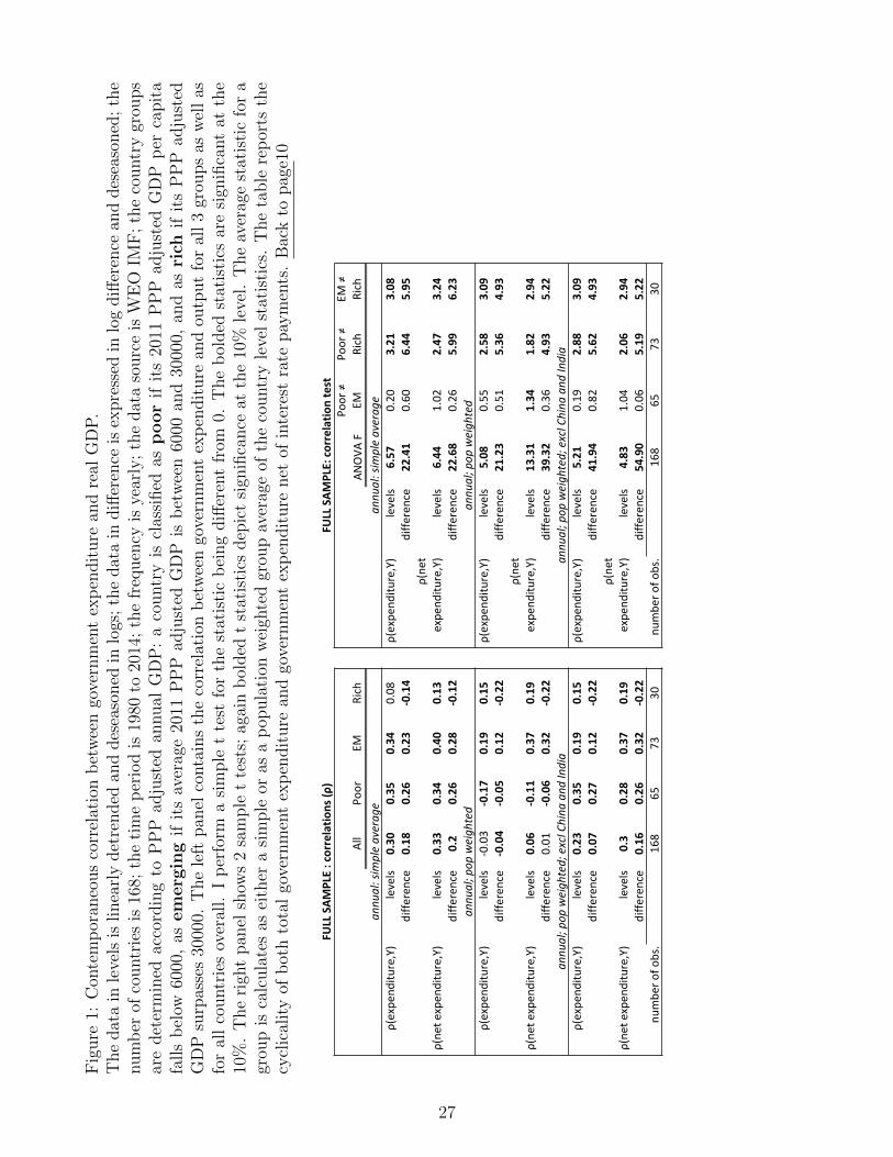
Fig

ure

1:C

onte

mp

oran

eous

corr

elat

ion

bet

wee

ngo

vern

men

tex

pen

dit

ure

and

real

GD

P.

The

dat

ain

leve

lsis

linea

rly

det

rended

and

des

easo

ned

inlo

gs;

the

dat

ain

diff

eren

ceis

expre

ssed

inlo

gdiff

eren

cean

ddes

easo

ned

;th

enum

ber

ofco

untr

ies

is16

8;th

eti

me

per

iod

is19

80to

2014

;th

efr

equen

cyis

year

ly;

the

dat

aso

urc

eis

WE

OIM

F;

the

countr

ygr

oups

are

det

erm

ined

acco

rdin

gto

PP

Pad

just

edan

nual

GD

P:

aco

untr

yis

clas

sified

asp

oor

ifit

s20

11P

PP

adju

sted

GD

Pp

erca

pit

afa

lls

bel

ow60

00,

asem

erg

ing

ifit

sav

erag

e20

11P

PP

adju

sted

GD

Pis

bet

wee

n60

00an

d30

000,

and

asri

chif

its

PP

Pad

just

edG

DP

surp

asse

s30

000.

The

left

pan

elco

nta

ins

the

corr

elat

ion

bet

wee

ngo

vern

men

tex

pen

dit

ure

and

outp

ut

for

all

3gr

oups

asw

ell

asfo

ral

lco

untr

ies

over

all.

Ip

erfo

rma

sim

ple

tte

stfo

rth

est

atis

tic

bei

ng

diff

eren

tfr

om0.

The

bol

ded

stat

isti

csar

esi

gnifi

cant

atth

e10

%.

The

righ

tpan

elsh

ows

2sa

mple

tte

sts;

agai

nb

olded

tst

atis

tics

dep

ict

sign

ifica

nce

atth

e10

%le

vel.

The

aver

age

stat

isti

cfo

ra

grou

pis

calc

ula

tes

asei

ther

asi

mple

oras

ap

opula

tion

wei

ghte

dgr

oup

aver

age

ofth

eco

untr

yle

vel

stat

isti

cs.

The

table

rep

orts

the

cycl

ical

ity

ofb

oth

tota

lgo

vern

men

tex

pen

dit

ure

and

gove

rnm

ent

exp

endit

ure

net

ofin

tere

stra

tepay

men

ts.

Bac

kto

pag

e10

All

Poor

EMRich

ANOVA

/FPo

or/≠/

EM/

Poor/≠/

Rich

EM/≠/

Rich

ρ(expe

nditu

re,Y)

levels

0.30

0.35

0.34

0.08

ρ(expe

nditu

re,Y)

levels

6.57

0.20

3.21

3.08

diffe

rence

0.18

0.26

0.23

+0.14

diffe

rence

22.41

0.60

6.44

5.95

ρ(ne

t/expen

diture,Y)

levels

0.33

0.34

0.40

0.13

ρ(ne

t/expe

nditu

re,Y)

levels

6.44

1.02

2.47

3.24

diffe

rence

0.2

0.26

0.28

+0.12

diffe

rence

22.68

0.26

5.99

6.23

ρ(expe

nditu

re,Y)

levels

G0.03

+0.17

0.19

0.15

ρ(expe

nditu

re,Y)

levels

5.08

0.55

2.58

3.09

diffe

rence

+0.04

+0.05

0.12

+0.22

diffe

rence

21.23

0.51

5.36

4.93

ρ(ne

t/expen

diture,Y)

levels

0.06

+0.11

0.37

0.19

ρ(ne

t/expe

nditu

re,Y)

levels

13.31

1.34

1.82

2.94

diffe

rence

0.01

+0.06

0.32

+0.22

diffe

rence

39.32

0.36

4.93

5.22

ρ(expe

nditu

re,Y)

levels

0.23

0.35

0.19

0.15

ρ(expe

nditu

re,Y)

levels

5.21

0.19

2.88

3.09

diffe

rence

0.07

0.27

0.12

+0.22

diffe

rence

41.94

0.82

5.62

4.93

ρ(ne

t/expen

diture,Y)

levels

0.3

0.28

0.37

0.19

ρ(ne

t/expe

nditu

re,Y)

levels

4.83

1.04

2.06

2.94

diffe

rence

0.16

0.26

0.32

+0.22

diffe

rence

54.90

0.06

5.19

5.22

numbe

r/of/o

bs.

168

6573

30nu

mbe

r/of/o

bs.

168

6573

30

annu

al;&pop

&weigh

ted

annu

al;&pop

&weigh

ted;&excl&China

&and

&India

FULL0SAM

PLE0:0correlatio

ns0(ρ

)

annu

al:&sim

ple&averag

e

annu

al;&pop

&weigh

ted

annu

al;&pop

&weigh

ted;&excl&China

&and

&India

FULL0SAM

PLE:0correlatio

n0test

annu

al:&sim

ple&averag

e

27

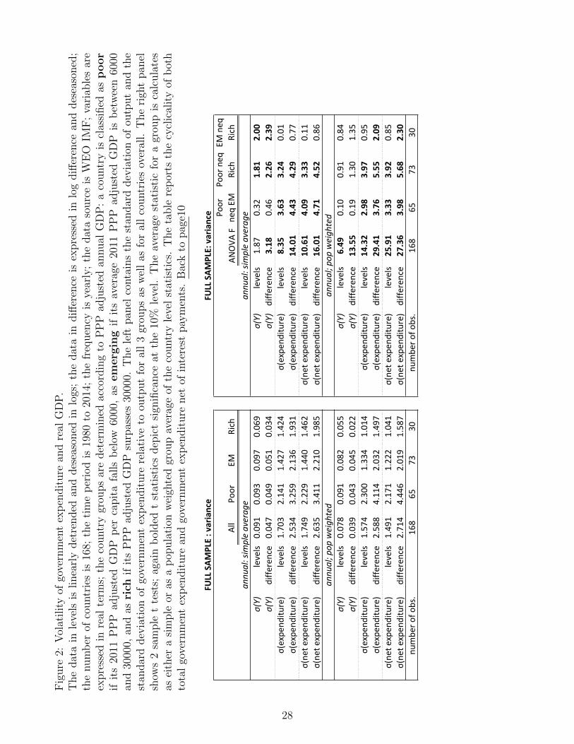
Fig

ure

2:V

olat

ilit

yof

gove

rnm

ent

exp

endit

ure

and

real

GD

P.

The

dat

ain

leve

lsis

linea

rly

det

rended

and

des

easo

ned

inlo

gs;

the

dat

ain

diff

eren

ceis

expre

ssed

inlo

gdiff

eren

cean

ddes

easo

ned

;th

enum

ber

ofco

untr

ies

is16

8;th

eti

me

per

iod

is19

80to

2014

;th

efr

equen

cyis

year

ly;

the

dat

aso

urc

eis

WE

OIM

F;

vari

able

sar

eex

pre

ssed

inre

alte

rms;

the

countr

ygr

oups

are

det

erm

ined

acco

rdin

gto

PP

Pad

just

edan

nual

GD

P:

aco

untr

yis

clas

sified

asp

oor

ifit

s20

11P

PP

adju

sted

GD

Pp

erca

pit

afa

lls

bel

ow60

00,

asem

erg

ing

ifit

sav

erag

e20

11P

PP

adju

sted

GD

Pis

bet

wee

n60

00an

d30

000,

and

asri

chif

its

PP

Pad

just

edG

DP

surp

asse

s30

000.

The

left

pan

elco

nta

ins

the

stan

dar

ddev

iati

onof

outp

ut

and

the

stan

dar

ddev

iati

onof

gove

rnm

ent

exp

endit

ure

rela

tive

toou

tput

for

all

3gr

oups

asw

ell

asfo

ral

lco

untr

ies

over

all.

The

righ

tpan

elsh

ows

2sa

mple

tte

sts;

agai

nb

olded

tst

atis

tics

dep

ict

sign

ifica

nce

atth

e10

%le

vel.

The

aver

age

stat

isti

cfo

ra

grou

pis

calc

ula

tes

asei

ther

asi

mple

oras

ap

opula

tion

wei

ghte

dgr

oup

aver

age

ofth

eco

untr

yle

vel

stat

isti

cs.

The

table

rep

orts

the

cycl

ical

ity

ofb

oth

tota

lgo

vern

men

tex

pen

dit

ure

and

gove

rnm

ent

exp

endit

ure

net

ofin

tere

stpay

men

ts.

Bac

kto

pag

e10

All

Poor

EMRich

ANOVA

/FPo

or/

neq/EM

/Po

or/neq

/Rich

EM/neq

/Rich

σ(Y)

levels

0.091

0.093

0.097

0.069

σ(Y)

levels

1.87

0.32

1.81

2.00

σ(Y)

diffe

rence

0.047

0.049

0.051

0.034

σ(Y)

diffe

rence

3.18

0.46

2.26

2.39

σ(expe

nditu

re)/

levels

1.703

2.141

1.427

1.424

σ(expe

nditu

re)/

levels

8.35

3.63

3.24

0.01

σ(expe

nditu

re)/

diffe

rence

2.534

3.259

2.136

1.931

σ(expe

nditu

re)/

diffe

rence

14.01

4.43

4.29

0.77

σ(ne

t/expen

diture)/

levels

1.749

2.229

1.440

1.462

σ(ne

t/expen

diture)/

levels

10.61

4.09

3.33

0.11

σ(ne

t/expen

diture)/

diffe

rence

2.635

3.411

2.210

1.985

σ(ne

t/expen

diture)

diffe

rence

16.01

4.71

4.52

0.86

σ(Y)

levels

0.078

0.091

0.082

0.055

σ(Y)

levels

6.49

0.10

0.91

0.84

σ(Y)

diffe

rence

0.039

0.043

0.045

0.022

σ(Y)

diffe

rence

13.55

0.19

1.30

1.35

σ(expe

nditu

re)

levels

1.574

2.300

1.334

1.014

σ(expe

nditu

re)/

levels

14.32

2.98

3.97

0.95

σ(expe

nditu

re)

diffe

rence

2.588

4.114

2.032

1.497

σ(expe

nditu

re)/

diffe

rence

29.41

3.76

5.55

2.09

σ(ne

t/expen

diture)

levels

1.491

2.171

1.222

1.041

σ(ne

t/expen

diture)

levels

25.91

3.33

3.92

0.85

σ(ne

t/expen

diture)

diffe

rence

2.714

4.446

2.019

1.587

σ(ne

t/expen

diture)/

diffe

rence

27.36

3.98

5.68

2.30

numbe

r/of/o

bs.

168

6573

30nu

mbe

r/of/o

bs.

168

6573

30

annu

al;*pop

*weigh

ted

annu

al;*pop

*weigh

ted

FULL/SAM

PLE/:/variance

FULL/SAM

PLE:/variance

annu

al:*sim

ple*averag

ean

nual:*sim

ple*averag

e

28

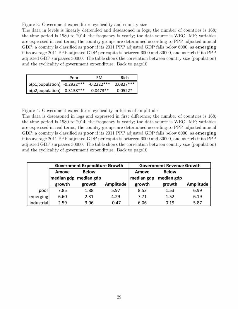
Figure 3: Government expenditure cyclicality and country sizeThe data in levels is linearly detrended and deseasoned in logs; the number of countries is 168;the time period is 1980 to 2014; the frequency is yearly; the data source is WEO IMF; variablesare expressed in real terms; the country groups are determined according to PPP adjusted annualGDP: a country is classified as poor if its 2011 PPP adjusted GDP falls below 6000, as emergingif its average 2011 PPP adjusted GDP per capita is between 6000 and 30000, and as rich if its PPPadjusted GDP surpasses 30000. The table shows the correlation between country size (population)and the cyclicality of government expenditure. Back to page10

Poor EM Richρ(ρ1,population) 50.2922*** 50.2222*** 0.0827***ρ(ρ2,population) 50.3138*** 50.0473** 0.0522*

Figure 4: Government expenditure cyclicality in terms of amplitudeThe data is deseasoned in logs and expressed in first difference; the number of countries is 168;the time period is 1980 to 2014; the frequency is yearly; the data source is WEO IMF; variablesare expressed in real terms; the country groups are determined according to PPP adjusted annualGDP: a country is classified as poor if its 2011 PPP adjusted GDP falls below 6000, as emergingif its average 2011 PPP adjusted GDP per capita is between 6000 and 30000, and as rich if its PPPadjusted GDP surpasses 30000. The table shows the correlation between country size (population)and the cyclicality of government expenditure. Back to page10

Amove&median&gdp&growth

Below&median&gdp&growth Amplitude

Amove&median&gdp&growth

Below&median&gdp&growth Amplitude

poor 7.85 1.88 5.97 8.52 1.53 6.99emerging 6.60 2.31 4.29 7.71 1.52 6.19industrial 2.59 3.06 :0.47 6.06 0.19 5.87

Government&Expenditure&Growth Government&Revenue&Growth

29

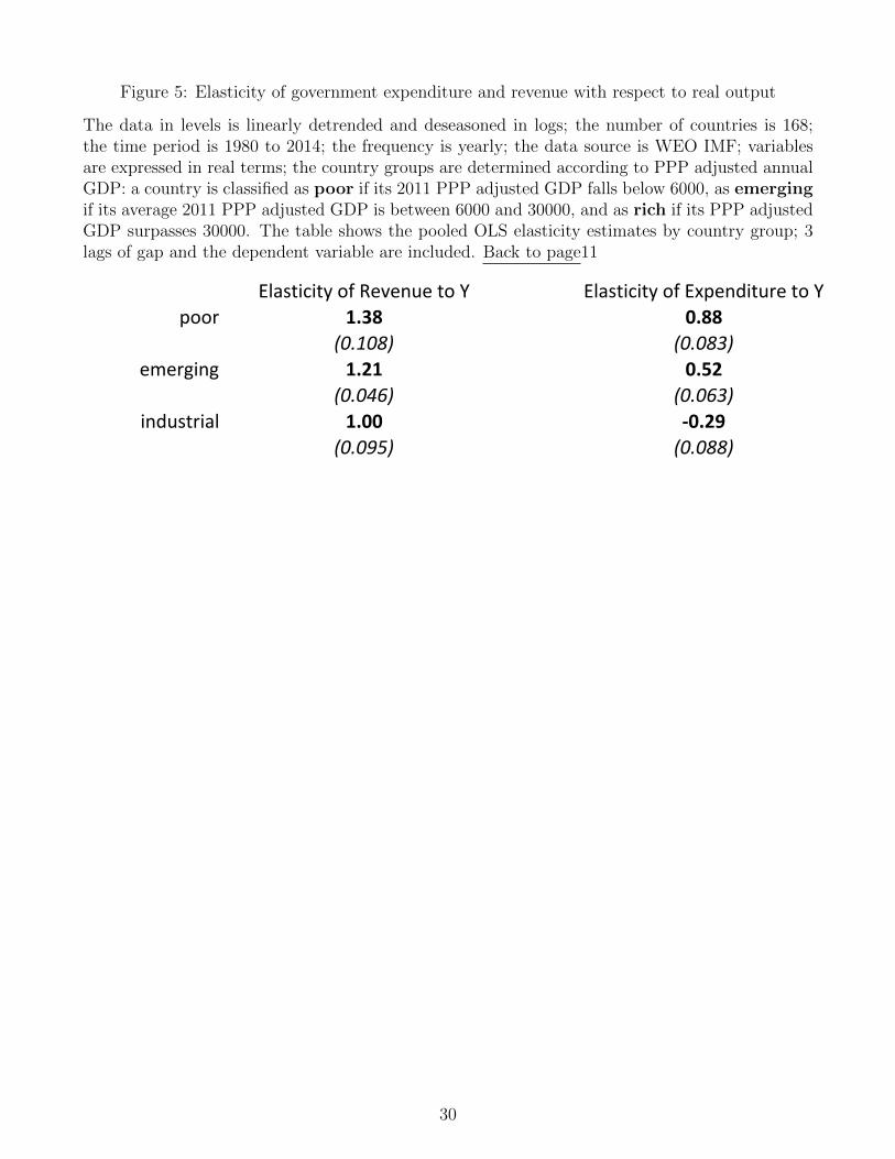
Figure 5: Elasticity of government expenditure and revenue with respect to real output

The data in levels is linearly detrended and deseasoned in logs; the number of countries is 168;the time period is 1980 to 2014; the frequency is yearly; the data source is WEO IMF; variablesare expressed in real terms; the country groups are determined according to PPP adjusted annualGDP: a country is classified as poor if its 2011 PPP adjusted GDP falls below 6000, as emergingif its average 2011 PPP adjusted GDP is between 6000 and 30000, and as rich if its PPP adjustedGDP surpasses 30000. The table shows the pooled OLS elasticity estimates by country group; 3lags of gap and the dependent variable are included. Back to page11

Elasticity)of)Revenue)to)Y Elasticity)of)Expenditure)to)Ypoor 1.38 0.88

(0.108) (0.083)emerging 1.21 0.52

(0.046) (0.063)industrial 1.00 (0.29

(0.095) (0.088)

30

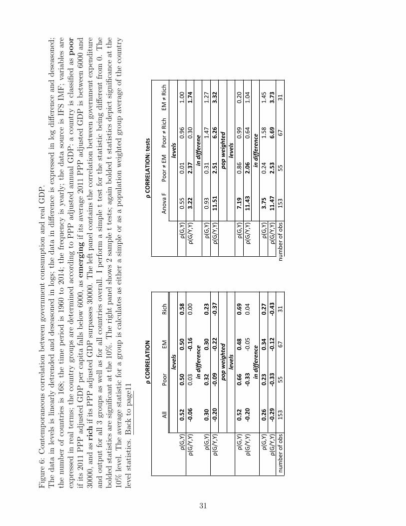
Fig

ure

6:C

onte

mp

oran

eous

corr

elat

ion

bet

wee

ngo

vern

men

tco

nsu

mpti

onan

dre

alG

DP

.T

he

dat

ain

leve

lsis

linea

rly

det

rended

and

des

easo

ned

inlo

gs;

the

dat

ain

diff

eren

ceis

expre

ssed

inlo

gdiff

eren

cean

ddes

easo

ned

;th

enum

ber

ofco

untr

ies

is16

8;th

eti

me

per

iod

is19

60to

2014

;th

efr

equen

cyis

year

ly;

the

dat

aso

urc

eis

IFS

IMF

;va

riab

les

are

expre

ssed

inre

alte

rms;

the

countr

ygr

oups

are

det

erm

ined

acco

rdin

gto

PP

Pad

just

edan

nual

GD

P:

aco

untr

yis

clas

sified

asp

oor

ifit

s20

11P

PP

adju

sted

GD

Pp

erca

pit

afa

lls

bel

ow60

00,

asem

erg

ing

ifit

sav

erag

e20

11P

PP

adju

sted

GD

Pis

bet

wee

n60

00an

d30

000,

and

asri

chif

its

PP

Pad

just

edG

DP

surp

asse

s30

000.

The

left

pan

elco

nta

ins

the

corr

elat

ion

bet

wee

ngo

vern

men

tex

pen

dit

ure

and

outp

ut

for

all

3gr

oups

asw

ell

asfo

ral

lco

untr

ies

over

all.

Ip

erfo

rma

sim

ple

tte

stfo

rth

est

atis

tic

bei

ng

diff

eren

tfr

om0.

The

bol

ded

stat

isti

csar

esi

gnifi

cant

atth

e10

%.

The

righ

tpan

elsh

ows

2sa

mple

tte

sts;

agai

nb

olded

tst

atis

tics

dep

ict

sign

ifica

nce

atth

e10

%le

vel.

The

aver

age

stat

isti

cfo

ra

grou

pis

calc

ula

tes

asei

ther

asi

mple

oras

ap

opula

tion

wei

ghte

dgr

oup

aver

age

ofth

eco

untr

yle

vel

stat

isti

cs.

Bac

kto

pag

e11

All

Poor

EMRich

Anova/F

Poor/≠/EM/

Poor/≠/Rich

EM/≠/Rich

ρ(G,Y)

0.52

0.50

0.50

0.58

ρ(G,Y)

0.55

0.01

0.96

1.00

ρ(G/

Y,Y)

&0.06

0.03

&0.16

0.00

ρ(G/

Y,Y)

3.22

2.37

0.30

1.74

ρ(G,Y)

0.30

0.32

0.30

0.23

ρ(G,Y)

0.93

0.31

1.47

1.27

ρ(G/

Y,Y)

&0.20

&0.09

&0.22

&0.37

ρ(G/

Y,Y)

11.51

2.51

6.26

3.32

ρ(G,Y)

0.52

0.66

0.48

0.69

ρ(G,Y)

7.19

0.86

0.99

0.20

ρ(G/

Y,Y)

&0.20

&0.33

D0.05

0.04

ρ(G/

Y,Y)

11.43

2.06

0.64

1.04

ρ(G,Y)

0.26

0.23

0.34

0.27

ρ(G,Y)

3.75

0.24

1.58

1.45

ρ(G/

Y,Y)

&0.29

&0.33

&0.12

&0.43

ρ(G/

Y,Y)

11.47

2.53

6.69

3.73

numbe

r/of/o

bs153

5567

31nu

mbe

r/of/o

bs153

5567

31

in#differen

ce

levels

ρ.CO

RRELAT

ION:.tests

levels

in#differen

e

pop#weigh

ted

in#differen

ce

levels

in#differen

ce

pop#weigh

ted

levels

ρ.CO

RRELAT

ION

31

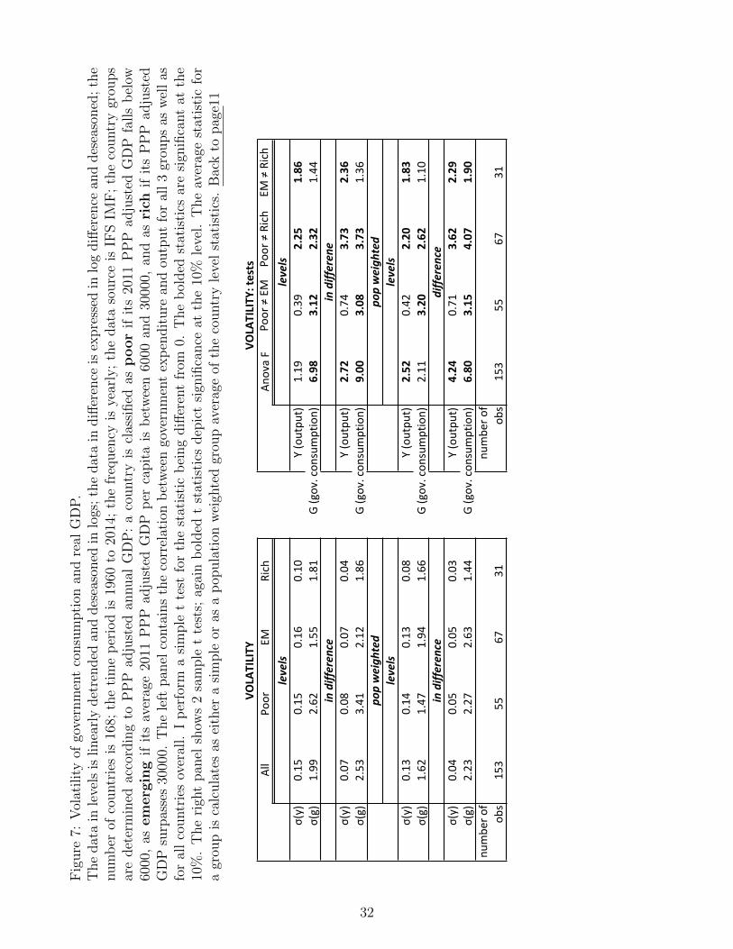
Fig

ure

7:V

olat

ilit

yof

gove

rnm

ent

consu

mpti

onan

dre

alG

DP

.T

he

dat

ain

leve

lsis

linea

rly

det

rended

and

des

easo

ned

inlo

gs;

the

dat

ain

diff

eren

ceis

expre

ssed

inlo

gdiff

eren

cean

ddes

easo

ned

;th

enum

ber

ofco

untr

ies

is16

8;th

eti

me

per

iod

is19

60to

2014

;th

efr

equen

cyis

year

ly;

the

dat

aso

urc

eis

IFS

IMF

;th

eco

untr

ygr

oups

are

det

erm

ined

acco

rdin

gto

PP

Pad

just

edan

nual

GD

P:

aco

untr

yis

clas

sified

asp

oor

ifit

s20

11P

PP

adju

sted

GD

Pfa

lls

bel

ow60

00,

asem

erg

ing

ifit

sav

erag

e20

11P

PP

adju

sted

GD

Pp

erca

pit

ais

bet

wee

n60

00an

d30

000,

and

asri

chif

its

PP

Pad

just

edG

DP

surp

asse

s30

000.

The

left

pan

elco

nta

ins

the

corr

elat

ion

bet

wee

ngo

vern

men

tex

pen

dit

ure

and

outp

ut

for

all

3gr

oups

asw

ell

asfo

ral

lco

untr

ies

over

all.

Ip

erfo

rma

sim

ple

tte

stfo

rth

est

atis

tic

bei

ng

diff

eren

tfr

om0.

The

bol

ded

stat

isti

csar

esi

gnifi

cant

atth

e10

%.

The

righ

tpan

elsh

ows

2sa

mple

tte

sts;

agai

nb

olded

tst

atis

tics

dep

ict

sign

ifica

nce

atth

e10

%le

vel.

The

aver

age

stat

isti

cfo

ra

grou

pis

calc

ula

tes

asei

ther

asi

mple

oras

ap

opula

tion

wei

ghte

dgr

oup

aver

age

ofth

eco

untr

yle

vel

stat

isti

cs.

Bac

kto

pag

e11

All

Poor

EMRich

Anova/F

Poor/≠/EM/

Poor/≠/Rich

EM/≠/Rich

σ(y)

0.15

0.15

0.16

0.10

Y/(outpu

t)1.19

0.39

2.25

1.86

σ(g)

1.99

2.62

1.55

1.81

G/(gov./con

sumption)

6.98

3.12

2.32

1.44

σ(y)

0.07

0.08

0.07

0.04

Y/(outpu

t)2.72

0.74

3.73

2.36

σ(g)

2.53

3.41

2.12

1.86

G/(gov./con

sumption)

9.00

3.08

3.73

1.36

σ(y)

0.13

0.14

0.13

0.08

Y/(outpu

t)2.52

0.42

2.20

1.83

σ(g)

1.62

1.47

1.94

1.66

G/(gov./con

sumption)

2.11

3.20

2.62

1.10

σ(y)

0.04

0.05

0.05

0.03

Y/(outpu

t)4.24

0.71

3.62

2.29

σ(g)

2.23

2.27

2.63

1.44

G/(gov./con

sumption)

6.80

3.15

4.07

1.90

numbe

r/of/

obs

153

5567

31nu

mbe

r/of/

obs

153

5567

31

VOLA

TILITY

:4tests

VOLA

TILITY

levels

in'differen

ce

levels

in'differen

e

pop'weigh

ted

levels

in'differen

ce

levels

diffe

rence

pop'weigh

ted

32

Figure 8: Contemporaneous correlation between the cyclical component of GDP and GovernmentExpenditure by group; The data in levels is linearly detrended and deseasoned in logs; the numberof countries is 168; the time period is 1980 to 2014; the frequency is yearly; the data source is WEOIMF; variables are expressed in real terms; the country groups are determined according to PPPadjusted annual GDP: a country is classified as poor if its 2011 PPP adjusted GDP falls below6000, as emerging if its average 2011 PPP adjusted GDP per capita is between 6000 and 30000,and as rich if its PPP adjusted GDP surpasses 30000. I report the rolling window correlation fora 5, 10 15 year window. Back to page12

-.4-.2

0.2

.4co

rr(gd

p, G

exp

endi

ture

)

1980 1990 2000 2010 2020year

5 yrs

-.20

.2.4

.6co

rr(gd

p, G

exp

endi

ture

)1995 2000 2005 2010 2015

year

poor eme-srich

15 yrs

-.20

.2.4

.6co

rr(gd

p, G

exp

endi

ture

)

1990 1995 2000 2005 2010 2015year

10 yrs

Corr(GDP, G expenditure)

33

Figure 9: Contemporaneous correlation between the cyclical component of GDP and Net Gov-ernment Expenditure by group; government expenditure is net of interest rate payments; Thedata in levels is linearly detrended and deseasoned in logs; the number of countries is 168; thetime period is 1980 to 2014; the frequency is yearly; the data source is WEO IMF; variables areexpressed in real terms; the country groups are determined according to PPP adjusted annualGDP: a country is classified as poor if its 2011 PPP adjusted GDP per capita falls below 6000,as emerging if its average 2011 PPP adjusted GDP is between 6000 and 30000, and as rich if itsPPP adjusted GDP surpasses 30000. I report the rolling window correlation for a 5, 10 15 yearwindow. Back to page12

-.50

.51

corr(

gdp,

G e

xpen

ditu

re)

1980 1990 2000 2010 2020year

5 yrs

-.20

.2.4

.6co

rr(gd

p, G

exp

endi

ture

)1995 2000 2005 2010 2015

year

poor eme-srich

15 yrs

-.20

.2.4

.6co

rr(gd

p, G

exp

endi

ture

)

1990 1995 2000 2005 2010 2015year

10 yrs

Corr(GDP, net G expenditure)

34

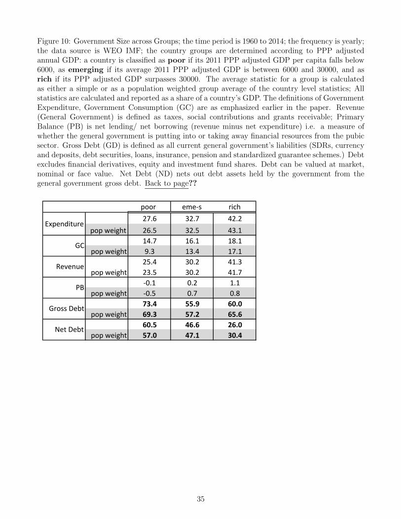
Figure 10: Government Size across Groups; the time period is 1960 to 2014; the frequency is yearly;the data source is WEO IMF; the country groups are determined according to PPP adjustedannual GDP: a country is classified as poor if its 2011 PPP adjusted GDP per capita falls below6000, as emerging if its average 2011 PPP adjusted GDP is between 6000 and 30000, and asrich if its PPP adjusted GDP surpasses 30000. The average statistic for a group is calculatedas either a simple or as a population weighted group average of the country level statistics; Allstatistics are calculated and reported as a share of a country’s GDP. The definitions of GovernmentExpenditure, Government Consumption (GC) are as emphasized earlier in the paper. Revenue(General Government) is defined as taxes, social contributions and grants receivable; PrimaryBalance (PB) is net lending/ net borrowing (revenue minus net expenditure) i.e. a measure ofwhether the general government is putting into or taking away financial resources from the pubicsector. Gross Debt (GD) is defined as all current general government’s liabilities (SDRs, currencyand deposits, debt securities, loans, insurance, pension and standardized guarantee schemes.) Debtexcludes financial derivatives, equity and investment fund shares. Debt can be valued at market,nominal or face value. Net Debt (ND) nets out debt assets held by the government from thegeneral government gross debt. Back to page??

poor eme-s rich27.6 32.7 42.2

popweight 26.5 32.5 43.114.7 16.1 18.1

popweight 9.3 13.4 17.125.4 30.2 41.3

popweight 23.5 30.2 41.7-0.1 0.2 1.1

popweight -0.5 0.7 0.873.4 55.9 60.0

popweight 69.3 57.2 65.660.5 46.6 26.0

popweight 57.0 47.1 30.4

GrossDebt

NetDebt

Expenditure

GC

Revenue

PB

35

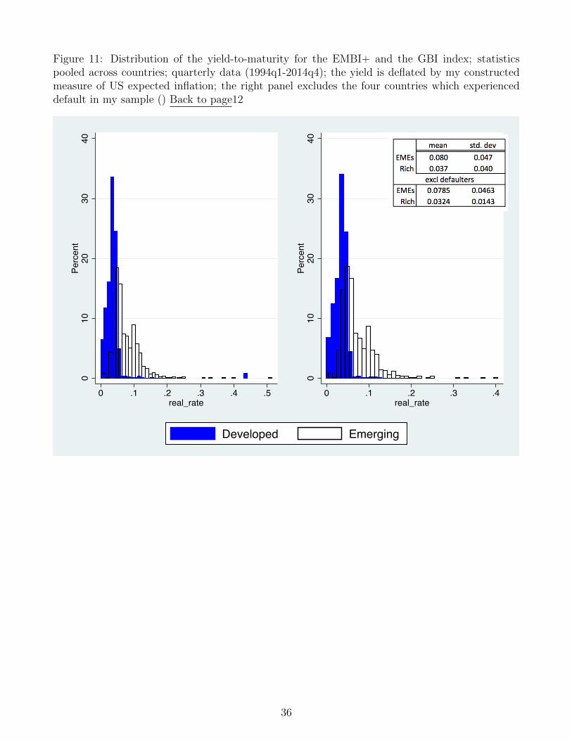
Figure 11: Distribution of the yield-to-maturity for the EMBI+ and the GBI index; statisticspooled across countries; quarterly data (1994q1-2014q4); the yield is deflated by my constructedmeasure of US expected inflation; the right panel excludes the four countries which experienceddefault in my sample () Back to page12

010

2030

40Percent

0 .1 .2 .3 .4 .5real_rate

010

2030

40Percent

0 .1 .2 .3 .4real_rate

Developed Emerging

36

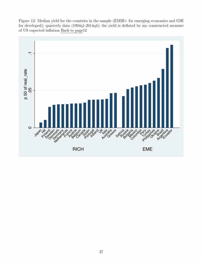
Figure 12: Median yield for the countries in the sample (EMBI+ for emerging economies and GBIfor developed); quarterly data (1994q1-2014q4); the yield is deflated by my constructed measureof US expected inflation Back to page12

0.0

5.1

p 50

of r

eal_

rate

RICH EME

Japa

n HK

Finland

Sweden

Denmark

German

y

Netherl

ands

France

Austria

Belgium

Canad

aSpa

in

Portug

al

Irelan

d UKIta

ly

Austra

lia

Greece

SafricaRus

sia

Bulgari

a

Mexico

ColombiaPeru

Turke

y

Philipp

ines

UkraineBraz

il

Argenti

na

Ecuad

or

37

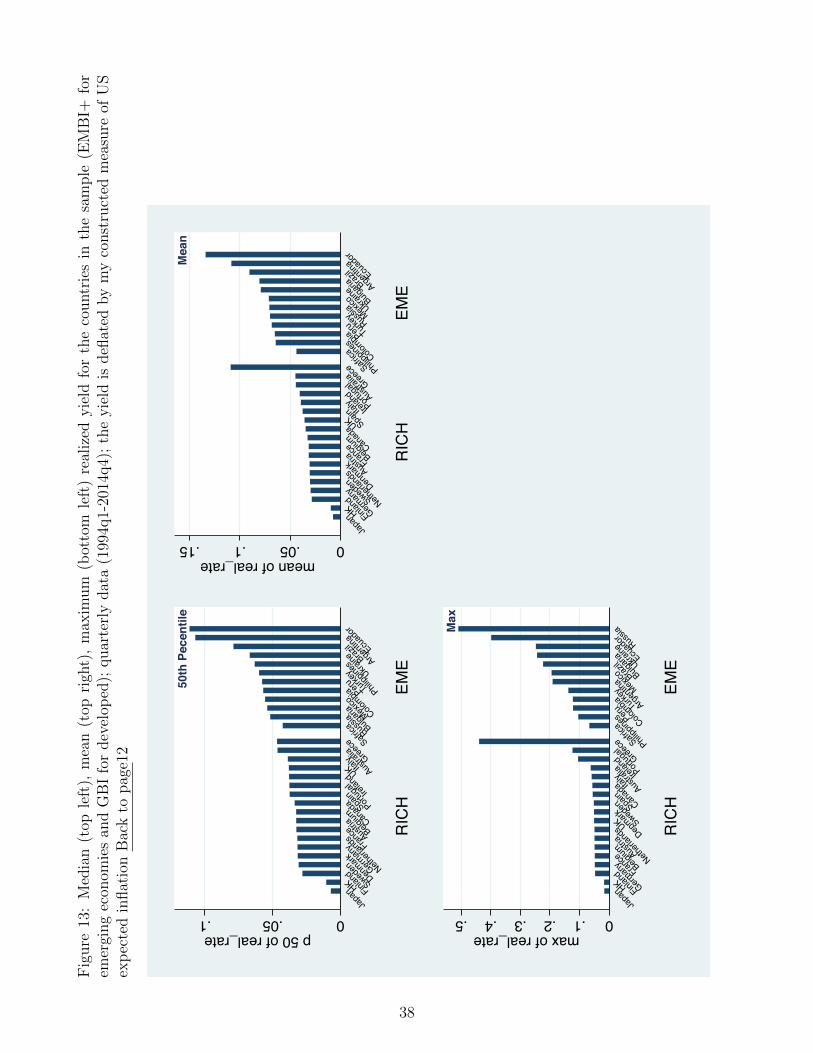
Fig

ure

13:

Med

ian

(top

left

),m

ean

(top

righ

t),

max

imum

(bot

tom

left

)re

aliz

edyie

ldfo

rth

eco

untr

ies

inth

esa

mple

(EM

BI+

for

emer

ging

econ

omie

san

dG

BI

for

dev

elop

ed);

quar

terl

ydat

a(1

994q

1-20

14q4)

;th

eyie

ldis

defl

ated

by

my

const

ruct

edm

easu

reof

US

exp

ecte

din

flat

ion

Bac

kto

pag

e 12

0.05.1p 50 of real_rate

RIC

HEM

E

Japa

n HKFinla

ndSwed

enDen

markGerm

any

Netherl

ands France Austria Belgium Canad

a Spain

Portug

al Irelan

d UK Italy

Austra

lia Greece Safrica Russia Bulgari

aMex

icoColo

mbia Peru Turke

y

Philipp

ines

Ukraine Braz

il

Argenti

naEcu

ador

50th

Pec

entil

e

0.05.1.15mean of real_rate

RIC

HEM

E

Japa

n HKFinla

ndGerm

any

Sweden

Netherl

ands

Denmark Aus

tria France

Belgium Canad

a UK Spain Italy Ire

land

Portug

alAus

tralia Greece Safrica

Philipp

ines

Colombia Peru Turke

yRus

sia Mexico Ukraine Bulgari

a Brazil

Argenti

naEcu

adorM

ean

0.1.2.3.4.5max of real_rate

RIC

HEM

E

Japa

n HKFinla

ndGerm

any

France

Belgium Austria

Netherl

andsUK

Denmark Swed

en Spain

Canad

a Italy

Austra

lia Irelan

dPort

ugal

Greece Safrica

Philipp

ines Peru

Colombia Turke

yArge

ntina Mexico Braz

ilBulg

aria

Ukraine Ecuad

or RussiaM

ax

38

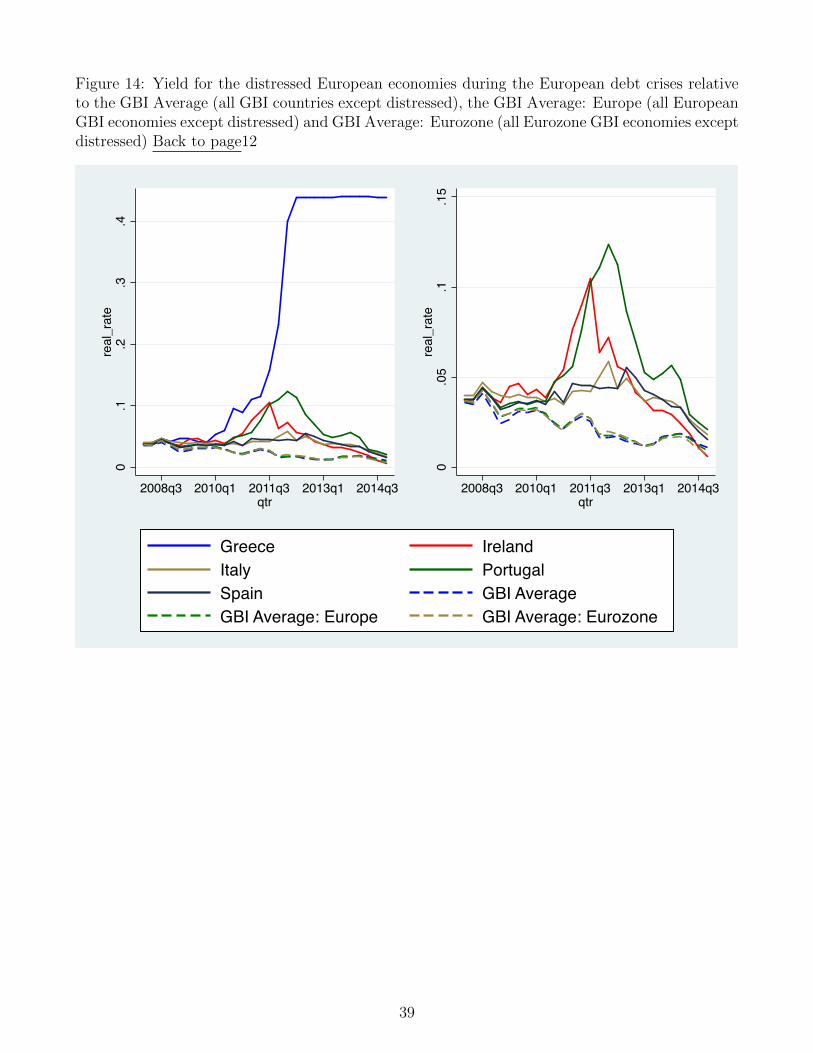
Figure 14: Yield for the distressed European economies during the European debt crises relativeto the GBI Average (all GBI countries except distressed), the GBI Average: Europe (all EuropeanGBI economies except distressed) and GBI Average: Eurozone (all Eurozone GBI economies exceptdistressed) Back to page12

0.1

.2.3

.4re

al_r

ate

2008q3 2010q1 2011q3 2013q1 2014q3qtr

0.0

5.1

.15

real

_rat

e

2008q3 2010q1 2011q3 2013q1 2014q3qtr

Greece IrelandItaly PortugalSpain GBI AverageGBI Average: Europe GBI Average: Eurozone

39

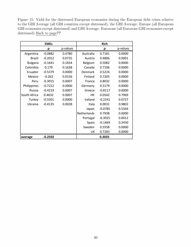
Figure 15: Yield for the distressed European economies during the European debt crises relativeto the GBI Average (all GBI countries except distressed), the GBI Average: Europe (all EuropeanGBI economies except distressed) and GBI Average: Eurozone (all Eurozone GBI economies exceptdistressed) Back to page??

! p-values ! p-valuesArgentina -0.0882 0.4780 Australia 0.7181 0.0000

Brazil -0.2012 0.0735 Austria 0.4806 0.0001Bulgaria -0.1641 0.1654 Belgium 0.5082 0.0000

Colombia 0.179 0.1638 Canada 0.7106 0.0000Ecuador -0.5379 0.0000 Denmark 0.5224 0.0000Mexico -0.263 0.0156 Finland 0.7205 0.0000

Peru -0.3915 0.0007 France 0.8032 0.0000Philippines -0.7212 0.0000 Germany 0.5179 0.0000

Russia -0.4219 0.0007 Greece -0.8117 0.0000SouthAfrica 0.4632 0.0007 HK 0.0542 0.7969

Turkey -0.5501 0.0000 Ireland -0.2241 0.0727Ukraine -0.4135 0.0028 Italy 0.0031 0.9802

Japan -0.0785 0.5344Netherlands 0.7938 0.0000

Portugal -0.3925 0.0012Spain -0.1469 0.2430

Sweden 0.5558 0.0000UK 0.7283 0.0000

average -0.2592 0.3035

EMEs Rich

40

Figure 16: Country by country estimates of the effect of the first lag of the designated variable onthe safe rate with 2(SE) bands; table lists countries for which bands do not include 0. 14

41

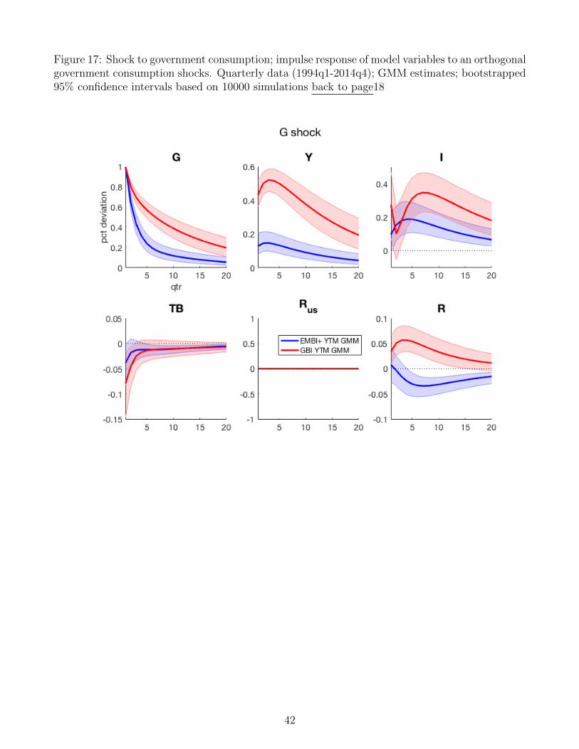
Figure 17: Shock to government consumption; impulse response of model variables to an orthogonalgovernment consumption shocks. Quarterly data (1994q1-2014q4); GMM estimates; bootstrapped95% confidence intervals based on 10000 simulations back to page18

42

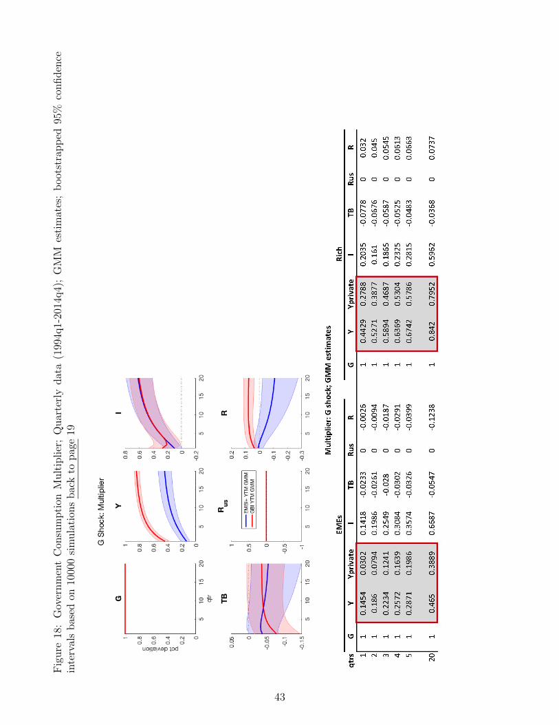
Fig

ure

18:

Gov

ernm

ent

Con

sum

pti

onM

ult

iplier

;Q

uar

terl

ydat

a(1

994q

1-20

14q4)

;G

MM

esti

mat

es;

boot

stra

pp

ed95

%co

nfiden

cein

terv

als

bas

edon

1000

0si

mula

tion

sbac

kto

pag

e19

43

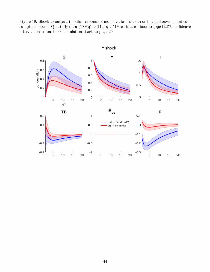
Figure 19: Shock to output; impulse response of model variables to an orthogonal government con-sumption shocks. Quarterly data (1994q1-2014q4); GMM estimates; bootstrapped 95% confidenceintervals based on 10000 simulations back to page 20

44

Figure 20: Multiplier Effect of an orthogonal Output Shock on the rest of the model variables;Quarterly data (1994q1-2014q4); GMM estimates; bootstrapped 95% confidence intervals basedon 10000 simulations back to page 20

45

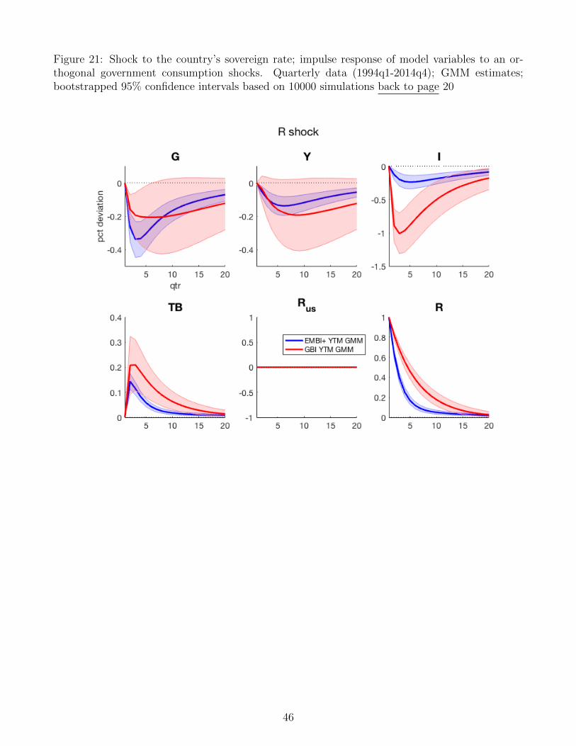
Figure 21: Shock to the country’s sovereign rate; impulse response of model variables to an or-thogonal government consumption shocks. Quarterly data (1994q1-2014q4); GMM estimates;bootstrapped 95% confidence intervals based on 10000 simulations back to page 20

46

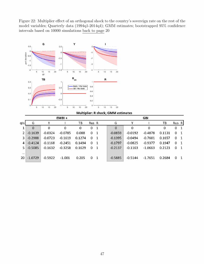
Figure 22: Multiplier effect of an orthogonal shock to the country’s sovereign rate on the rest of themodel variables; Quarterly data (1994q1-2014q4); GMM estimates; bootstrapped 95% confidenceintervals based on 10000 simulations back to page 20

47

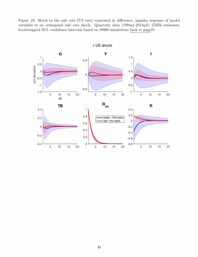
Figure 23: Shock to the safe rate (US rate) expressed in difference; impulse response of modelvariables to an orthogonal safe rate shock. Quarterly data (1994q1-2014q4); GMM estimates;bootstrapped 95% confidence intervals based on 10000 simulations back to page21

48

Figure 24: Government Shock’s Volatility by Country; author’s calculations based on identifyingorthogonal shocks from GMM estimates; Reduced form residuals in first difference; Quarterly data(1994q1-2014q4) back to page 21

0 0.05 0.1 0.15 0.2 0.25

MexicoSouth Africa

ColombiaBrazil

ArgentinaRussia

PhilippinesTurkey

PeruBulgariaEcuadorUkriane

0 0.01 0.02 0.03 0.04 0.05FranceDenmarkCanadaJapanBelgiumItalySwedenHKNetherlandsGermanyAustraliaUKSpainIrelandAustriaFinlandGreecePortugal

Estimated Volatility of Government Shocks (GMM)

0 0.05 0.1 0.15 0.2 0.250

5

10

15

20

EMEsRich

49

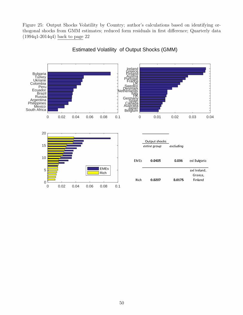
Figure 25: Output Shocks Volatility by Country; author’s calculations based on identifying or-thogonal shocks from GMM estimates; reduced form residuals in first difference; Quarterly data(1994q1-2014q4) back to page 22

0 0.02 0.04 0.06 0.08 0.1

South AfricaMexico

PhilippinesArgentina

RussiaBrazil

EcuadorPeru

ColombiaUkrianeTurkey

Bulgaria

0 0.01 0.02 0.03 0.04

BelgiumJapan

AustraliaCanada

SpainGermany

HKItaly

NetherlandsDenmarkSweden

UKFrance

PortugalAustriaFinlandGreeceIreland

Estimated Volatility of Output Shocks (GMM)

0 0.02 0.04 0.06 0.08 0.10

5

10

15

20

EMEsRich

50

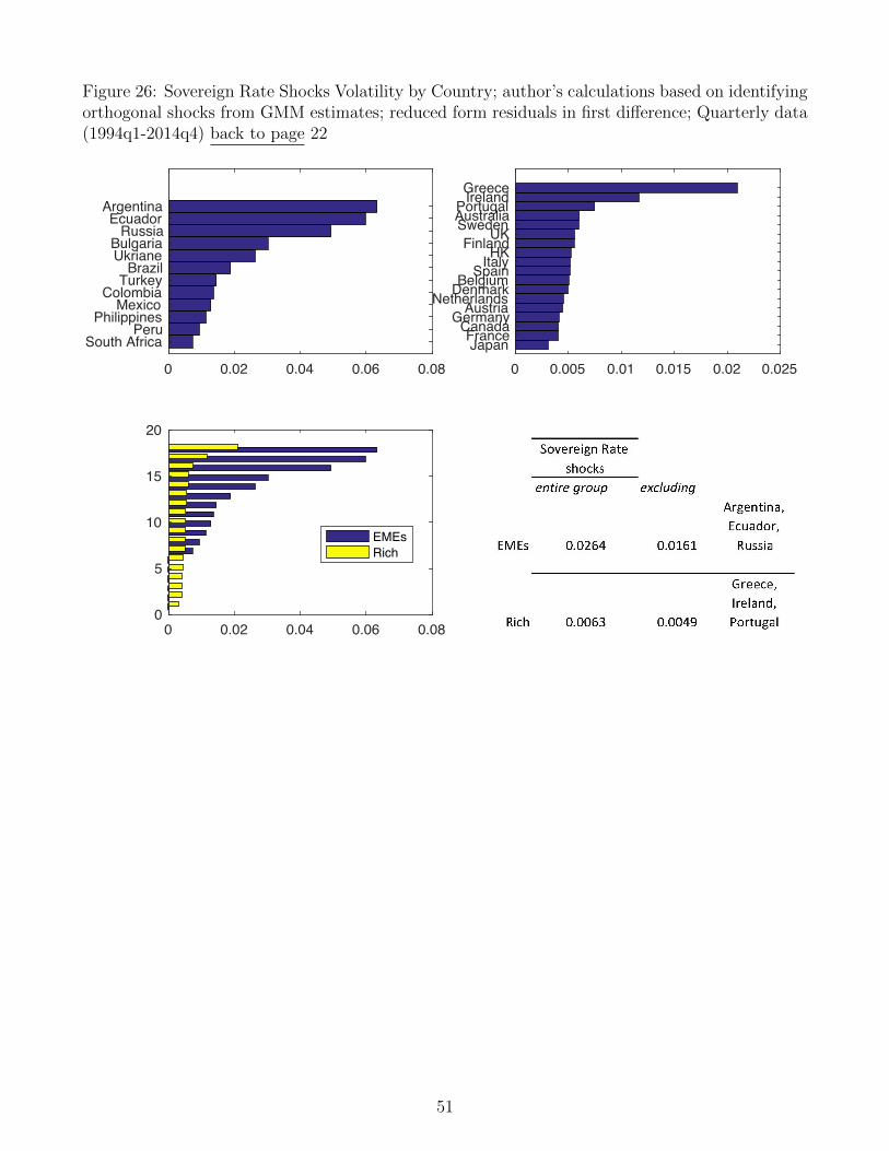
Figure 26: Sovereign Rate Shocks Volatility by Country; author’s calculations based on identifyingorthogonal shocks from GMM estimates; reduced form residuals in first difference; Quarterly data(1994q1-2014q4) back to page 22

0 0.02 0.04 0.06 0.08

South AfricaPeru

PhilippinesMexico

ColombiaTurkey

BrazilUkrianeBulgaria

RussiaEcuador

Argentina

0 0.005 0.01 0.015 0.02 0.025JapanFranceCanadaGermanyAustriaNetherlandsDenmarkBelgiumSpainItalyHKFinlandUKSwedenAustraliaPortugalIrelandGreece

Estimated Volatility of Output Shocks (GMM)

0 0.02 0.04 0.06 0.080

5

10

15

20

EMEsRich

51

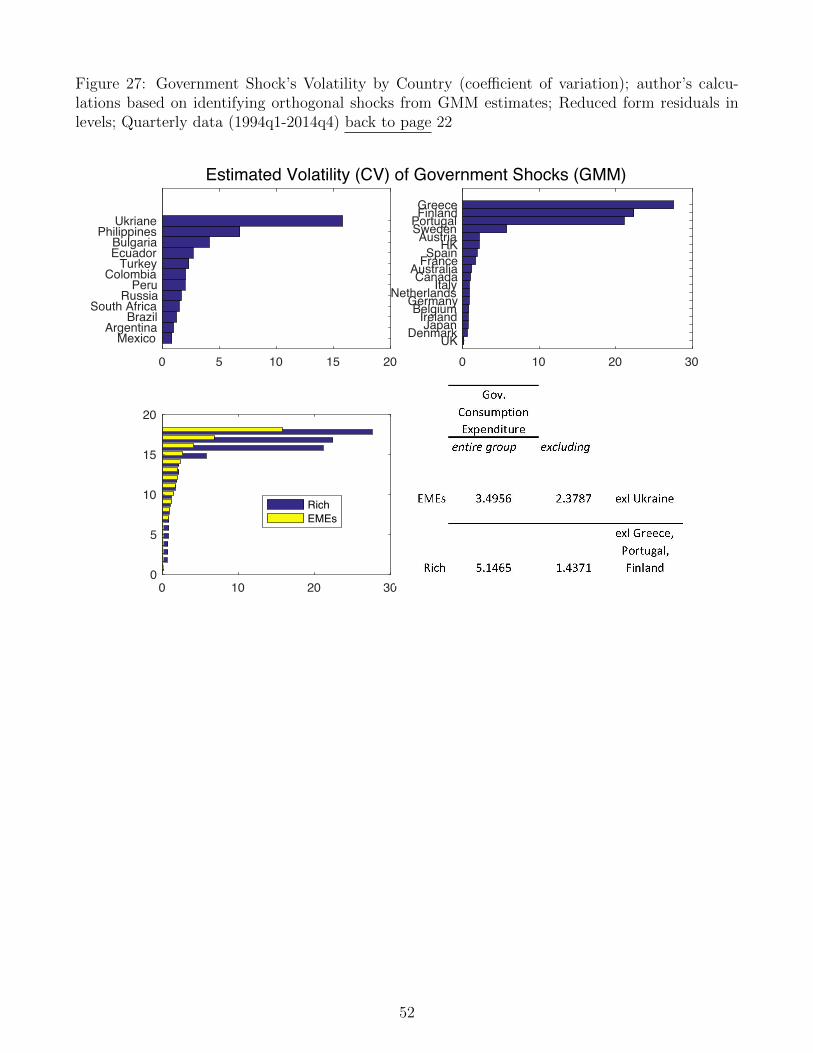
Figure 27: Government Shock’s Volatility by Country (coefficient of variation); author’s calcu-lations based on identifying orthogonal shocks from GMM estimates; Reduced form residuals inlevels; Quarterly data (1994q1-2014q4) back to page 22

Estimated Volatility (CV) of Government Shocks (GMM)

0 5 10 15 20

MexicoArgentina

BrazilSouth Africa

RussiaPeru

ColombiaTurkey

EcuadorBulgaria

PhilippinesUkriane

0 10 20 30UKDenmarkJapanIrelandBelgiumGermanyNetherlandsItalyCanadaAustraliaFranceSpainHKAustriaSwedenPortugalFinlandGreece

0 10 20 300

5

10

15

20

RichEMEs

52

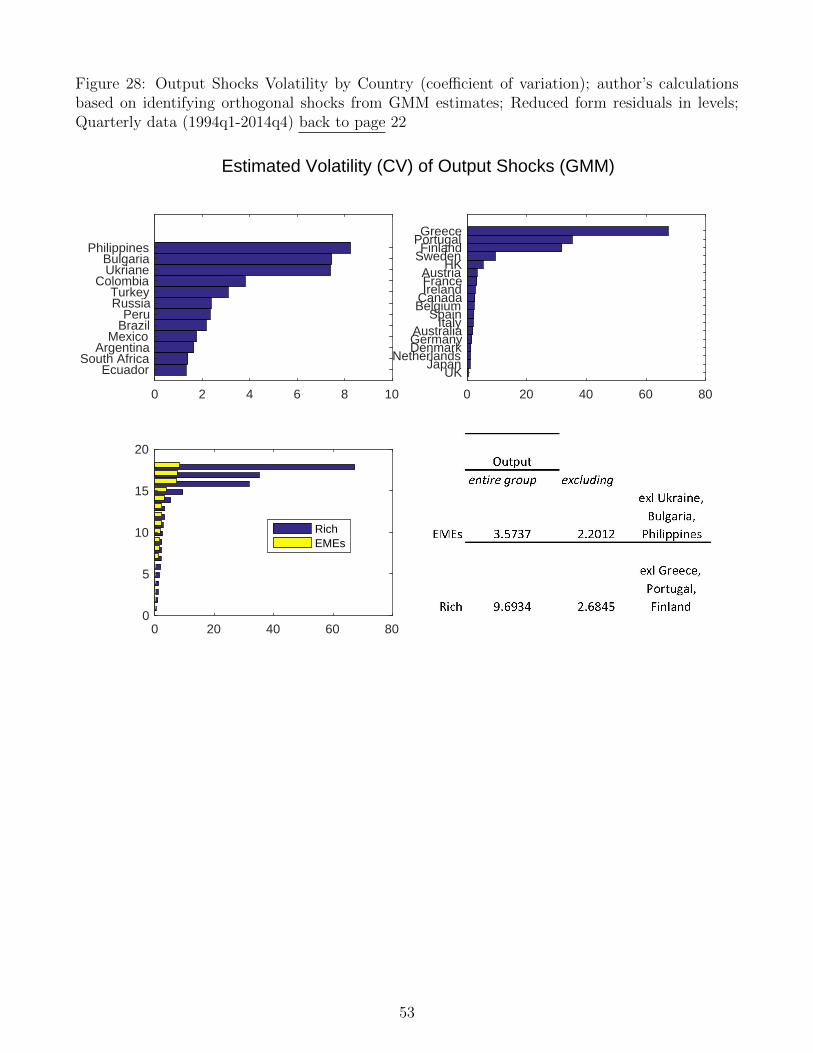
Figure 28: Output Shocks Volatility by Country (coefficient of variation); author’s calculationsbased on identifying orthogonal shocks from GMM estimates; Reduced form residuals in levels;Quarterly data (1994q1-2014q4) back to page 22

0 2 4 6 8 10

EcuadorSouth Africa

ArgentinaMexico

BrazilPeru

RussiaTurkey

ColombiaUkrianeBulgaria

Philippines

0 20 40 60 80

UKJapan

NetherlandsDenmarkGermanyAustralia

ItalySpain

BelgiumCanadaIrelandFranceAustria

HKSwedenFinland

PortugalGreece

Estimated Volatility (CV) of Output Shocks (GMM)

0 20 40 60 800

5

10

15

20

RichEMEs

53

Figure 29: Sovereign Rate Shocks Volatility by Country (coefficient of variation); author’s calcu-lations based on identifying orthogonal shocks from GMM estimates; Reduced form residuals infirst difference; Quarterly data (1994q1-2014q4) back to page 22

0 0.5 1 1.5 2

PeruMexicoTurkey

South AfricaBrazil

BulgariaColombia

PhilippinesEcuador

ArgentinaRussia

Ukriane

0 5 10 15 20 25UKJapanNetherlandsIrelandDenmarkCanadaGermanyBelgiumItalySpainHKAustraliaAustriaFranceSwedenFinlandPortugalGreece

Estimated Volatility (CV) of Output Shocks (GMM)

0 5 10 15 20 250

5

10

15

20

RichEMEs

Figure 30: AIC for GMM and fixed effects; p = 1 : 5 ??

lags developed EMEs developed EMEs1 "46.7119 "38.1053 "49.309 "41.29712 "46.1426 "37.4819 "48.9648 "40.59063 "45.0822 "37.0076 "48.5105 "39.89884 "45.9714 "37.758 "48.3197 "39.88565 "44.3563 "36.9211 "48.0406 "40.032

GMM FEAIC

54

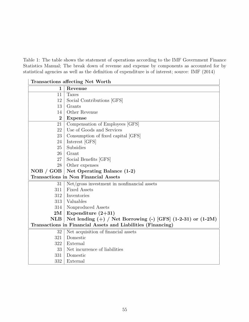
Table 1: The table shows the statement of operations according to the IMF Government FinanceStatistics Manual; The break down of revenue and expense by components as accounted for bystatistical agencies as well as the definition of expenditure is of interest; source: IMF (2014)

Transactions affecting Net Worth

1 Revenue11 Taxes12 Social Contributions [GFS]13 Grants14 Other Revenue2 Expense

21 Compensation of Employees [GFS]22 Use of Goods and Services23 Consumption of fixed capital [GFS]24 Interest [GFS]25 Subsidies26 Grant27 Social Benefits [GFS]28 Other expenses

NOB / GOB Net Operating Balance (1-2)Transactions in Non Financial Assets

31 Net/gross investment in nonfinancial assets311 Fixed Assets312 Inventories313 Valuables314 Nonproduced Assets2M Expenditure (2+31)

NLB Net lending (+) / Net Borrowing (-) [GFS] (1-2-31) or (1-2M)Transactions in Financial Assets and Liabilities (Financing)

32 Net acquisition of financial assets321 Domestic322 External33 Net incurrence of liabilities

331 Domestic332 External

55

Figure 31: Estimates of Ai=0,1; Dynamic panel data estimation, one-step difference GMM; quar-terly data; deseasoned; (1994q1-2014q4); Npanels = 30; standard errors clustered by country arereported in parenthesis; last three rows report the p-values for the Hansen test of overidentifyingrestrictions (H0: instruments are jointly valid i.e (1/N)Z ′U is mean 0, N is the number of panels)and the Arellano-Bond test for autocorrelation in the error (H0: error are not l-order serially cor-related i.e (1/N)EU ′−lU = 0) estimates shown for the base group (developed economies)back to page16

GC Y Inv TBY SafeR Sov.RGC 0.325*** 0.014 -0.150** 0.006

(0.069) (0.135) (0.053) (0.022)Y 0.955*** 0.222* 0.025

(0.113) (0.102) (0.016)Inv -0.135*** -0.035

(0.019) (0.019)TBY -0.021

(0.011)SafeR 0.056***

(0.007)Sov.R

L.GC 0.729*** -0.061 -0.421** 0.014 0.024*(0.059) (0.061) (0.151) (0.045) (0.009)

L.Y 0.246** 0.683*** -0.084 0.004 -0.029(0.072) (0.077) (0.138) (0.112) (0.015)

L.Inv -0.025 0.013 0.564*** 0.003 0.011**(0.017) (0.022) (0.048) (0.024) (0.004)

L.TBY -0.057 -0.062 -0.069 0.153 -0.008(0.044) (0.081) (0.097) (0.092) (0.010)

L.SafeR -0.073*** 0.097*** 0.212** -0.014 0.596*** -0.024(0.019) (0.017) (0.073) (0.019) (0.087) (0.014)

L.Sov.Rate -0.052 0.013 -0.542*** 0.003 0.943***(0.029) (0.042) (0.127) (0.042) (0.018)

N 1896 1896 1896 1896 82 1895hansenp 1.000 1.000 1.000 1.000 1.000

ar1p 0.028 0.003 0.003 0.086 0.049ar2p 0.436 0.751 0.023 0.653 0.946

56

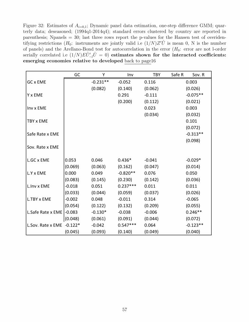
Figure 32: Estimates of Ai=0,1; Dynamic panel data estimation, one-step difference GMM; quar-terly data; deseasoned; (1994q1-2014q4); standard errors clustered by country are reported inparenthesis; Npanels = 30; last three rows report the p-values for the Hansen test of overiden-tifying restrictions (H0: instruments are jointly valid i.e (1/N)Z ′U is mean 0, N is the numberof panels) and the Arellano-Bond test for autocorrelation in the error (H0: error are not l-orderserially correlated i.e (1/N)EU ′−lU = 0) estimates shown for the interacted coefficients:emerging economies relative to developed back to page16

GC Y Inv TBY SafeR Sov.RGCxEME -0.231** -0.052 0.116 0.003

(0.082) (0.140) (0.062) (0.026)YxEME 0.291 -0.111 -0.075**

(0.200) (0.112) (0.021)InvxEME 0.023 0.003

(0.034) (0.032)TBYxEME 0.101

(0.072)SafeRatexEME -0.313**

(0.098)Sov.RatexEME

L.GCxEME 0.053 0.046 0.436* -0.041 -0.029*(0.069) (0.063) (0.162) (0.047) (0.014)

L.YxEME 0.000 0.049 -0.820** 0.076 0.050(0.083) (0.145) (0.230) (0.142) (0.036)

L.InvxEME -0.018 0.051 0.237*** 0.011 0.011(0.033) (0.044) (0.059) (0.037) (0.026)

L.TBYxEME -0.002 0.048 -0.011 0.314 -0.065(0.054) (0.122) (0.132) (0.209) (0.055)

L.SafeRatexEME -0.083 -0.130* -0.038 -0.006 0.246**(0.048) (0.061) (0.091) (0.044) (0.072)

L.Sov.RatexEME -0.122* -0.042 0.547*** 0.064 -0.123**(0.045) (0.093) (0.140) (0.049) (0.040)

57

Figure 33: Dynamic panel data estimation, one-step difference GMM; quarterly data; desea-soned; (1994q1-2014q4); Npanels = 30; standard errors clustered by country are reported inparenthesis; last three rows report the p-values for the Hansen test of overidentifying restric-tions (H0: instruments are jointly valid i.e (1/N)Z ′U is mean 0, N is the number of panels) andthe Arellano-Bond test for autocorrelation in the error (H0: error are not l-order serially corre-lated i.e (1/N)EU ′−lU = 0) Government response function to fundamentals across thetwo groups (developed and emerging); the first two columns show estimates basedon group by group estimation; last two columns show estimates for the whole samplewith developed economies being the base group. back to page 16

GC GCRich Emerging

L.GC 0.729*** 0.782*** 0.729*** L.GCxEME 0.053(0.060) (0.036) (0.059) (0.069)

L.Y 0.246** 0.247*** 0.246** L.YxEME 0.000(0.073) (0.043) (0.072) (0.083)

L.Inv -0.025 -0.043 -0.025 L.InvxEME -0.018(0.018) (0.029) (0.017) (0.033)

L.TBY -0.057 -0.059 -0.057 L.TBYxEME -0.002(0.044) (0.033) (0.044) (0.054)

L.SafeRate -0.073** -0.156** -0.073*** L.SafeRatexEME -0.083(0.019) (0.046) (0.019) (0.048)

L.Sov.Rate -0.052 -0.174*** -0.052 L.Sov.RatexEME -0.122*(0.030) (0.034) (0.029) (0.045)

N 1094 802 1896hansenp 1 1 1ar1p 0.001 0.04 0.028ar2p 0.078 0.549 0.436

GCJoint

GMMEstimates

58

Figure 34: Dynamic panel data estimation, one-step difference GMM; quarterly data; desea-soned; (1994q1-2014q4); Npanels = 30; standard errors clustered by country are reported inparenthesis; last three rows report the p-values for the Hansen test of overidentifying restrictions(H0: instruments are jointly valid i.e (1/N)Z ′U is mean 0, N is the number of panels) and theArellano-Bond test for autocorrelation in the error (H0: errors are not l-order serially correlatedi.e (1/N)EU ′−lU = 0) Government response function to fundamentals across the twogroups (developed and emerging); baseline estimation compared with estimates usingprivate real GDP back to page 17

Y=Yprivate Y=YprivateL.GC 0.729*** 0.773*** L.GCxEME 0.053 -0.048

(0.059) (0.094) (0.069) (0.116)L.Y 0.246** 0.209 L.YxEME 0.000 0.035

(0.072) (0.105) (0.083) (0.105)L.Inv -0.025 -0.026 L.InvxEME -0.018 -0.004

(0.017) (0.064) (0.033) (0.102)L.TBY -0.057 -0.115 L.TBYxEME -0.002 0.165

(0.044) (0.084) (0.054) (0.150)L.SafeRate -0.073*** -0.105* L.SafeRatexEME -0.083 -0.183

(0.019) (0.038) (0.048) (0.105)L.Sov.Rate -0.052 -0.067 L.Sov.RatexEME -0.122* -0.230*

(0.029) (0.067) (0.045) (0.102)N 1896 1896hansenp 1 1ar1p 0.028 0.034ar2p 0.436 0.445

GMMEstimates:GC

59

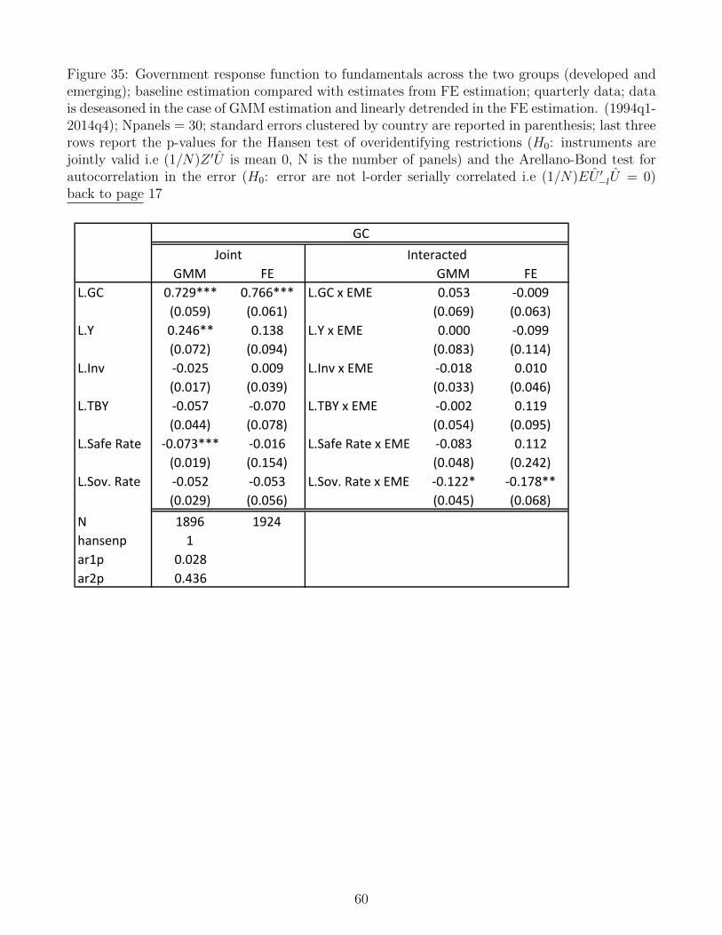
Figure 35: Government response function to fundamentals across the two groups (developed andemerging); baseline estimation compared with estimates from FE estimation; quarterly data; datais deseasoned in the case of GMM estimation and linearly detrended in the FE estimation. (1994q1-2014q4); Npanels = 30; standard errors clustered by country are reported in parenthesis; last threerows report the p-values for the Hansen test of overidentifying restrictions (H0: instruments arejointly valid i.e (1/N)Z ′U is mean 0, N is the number of panels) and the Arellano-Bond test forautocorrelation in the error (H0: error are not l-order serially correlated i.e (1/N)EU ′−lU = 0)back to page 17

GMM FE GMM FEL.GC 0.729*** 0.766*** L.GCxEME 0.053 -0.009

(0.059) (0.061) (0.069) (0.063)L.Y 0.246** 0.138 L.YxEME 0.000 -0.099

(0.072) (0.094) (0.083) (0.114)L.Inv -0.025 0.009 L.InvxEME -0.018 0.010

(0.017) (0.039) (0.033) (0.046)L.TBY -0.057 -0.070 L.TBYxEME -0.002 0.119

(0.044) (0.078) (0.054) (0.095)L.SafeRate -0.073*** -0.016 L.SafeRatexEME -0.083 0.112

(0.019) (0.154) (0.048) (0.242)L.Sov.Rate -0.052 -0.053 L.Sov.RatexEME -0.122* -0.178**

(0.029) (0.056) (0.045) (0.068)N 1896 1924hansenp 1ar1p 0.028ar2p 0.436

GCJoint Interacted

60

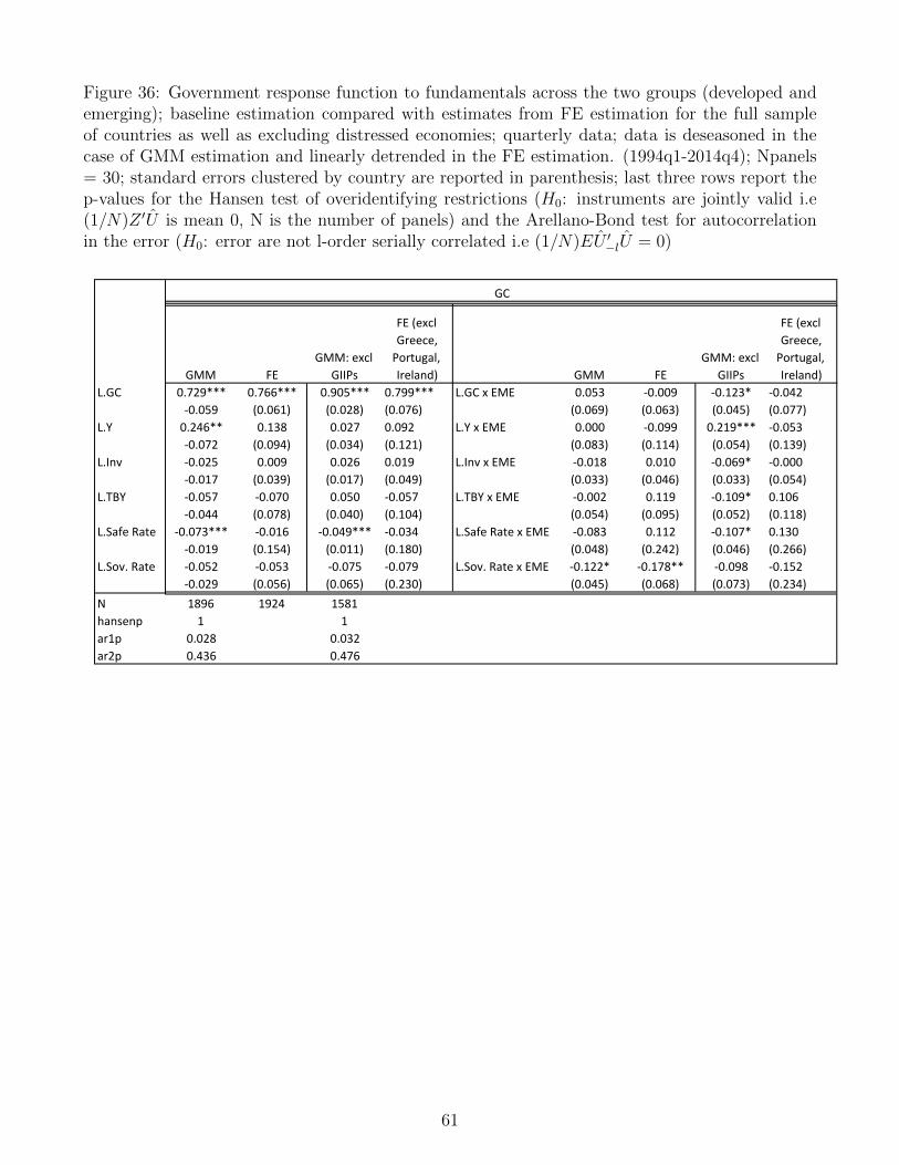
Figure 36: Government response function to fundamentals across the two groups (developed andemerging); baseline estimation compared with estimates from FE estimation for the full sampleof countries as well as excluding distressed economies; quarterly data; data is deseasoned in thecase of GMM estimation and linearly detrended in the FE estimation. (1994q1-2014q4); Npanels= 30; standard errors clustered by country are reported in parenthesis; last three rows report thep-values for the Hansen test of overidentifying restrictions (H0: instruments are jointly valid i.e(1/N)Z ′U is mean 0, N is the number of panels) and the Arellano-Bond test for autocorrelationin the error (H0: error are not l-order serially correlated i.e (1/N)EU ′−lU = 0)

GMM FEGMM:excl

GIIPs

FE(exclGreece,Portugal,Ireland) GMM FE

GMM:exclGIIPs

FE(exclGreece,Portugal,Ireland)

L.GC 0.729*** 0.766*** 0.905*** 0.799*** L.GCxEME 0.053 -0.009 -0.123* -0.042-0.059 (0.061) (0.028) (0.076) (0.069) (0.063) (0.045) (0.077)

L.Y 0.246** 0.138 0.027 0.092 L.YxEME 0.000 -0.099 0.219*** -0.053-0.072 (0.094) (0.034) (0.121) (0.083) (0.114) (0.054) (0.139)

L.Inv -0.025 0.009 0.026 0.019 L.InvxEME -0.018 0.010 -0.069* -0.000-0.017 (0.039) (0.017) (0.049) (0.033) (0.046) (0.033) (0.054)

L.TBY -0.057 -0.070 0.050 -0.057 L.TBYxEME -0.002 0.119 -0.109* 0.106-0.044 (0.078) (0.040) (0.104) (0.054) (0.095) (0.052) (0.118)

L.SafeRate -0.073*** -0.016 -0.049*** -0.034 L.SafeRatexEME -0.083 0.112 -0.107* 0.130-0.019 (0.154) (0.011) (0.180) (0.048) (0.242) (0.046) (0.266)

L.Sov.Rate -0.052 -0.053 -0.075 -0.079 L.Sov.RatexEME -0.122* -0.178** -0.098 -0.152-0.029 (0.056) (0.065) (0.230) (0.045) (0.068) (0.073) (0.234)

N 1896 1924 1581hansenp 1 1ar1p 0.028 0.032ar2p 0.436 0.476

GCJoint Joint Interactions

61

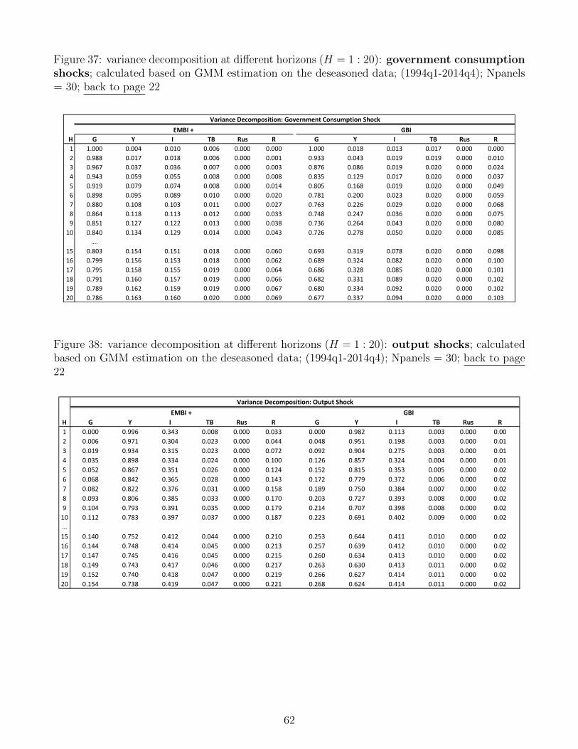
Figure 37: variance decomposition at different horizons (H = 1 : 20): government consumptionshocks; calculated based on GMM estimation on the deseasoned data; (1994q1-2014q4); Npanels= 30; back to page 22

H G Y I TB Rus R G Y I TB Rus R1 1.000 0.004 0.010 0.006 0.000 0.000 1.000 0.018 0.013 0.017 0.000 0.0002 0.988 0.017 0.018 0.006 0.000 0.001 0.933 0.043 0.019 0.019 0.000 0.0103 0.967 0.037 0.036 0.007 0.000 0.003 0.876 0.086 0.019 0.020 0.000 0.0244 0.943 0.059 0.055 0.008 0.000 0.008 0.835 0.129 0.017 0.020 0.000 0.0375 0.919 0.079 0.074 0.008 0.000 0.014 0.805 0.168 0.019 0.020 0.000 0.0496 0.898 0.095 0.089 0.010 0.000 0.020 0.781 0.200 0.023 0.020 0.000 0.0597 0.880 0.108 0.103 0.011 0.000 0.027 0.763 0.226 0.029 0.020 0.000 0.0688 0.864 0.118 0.113 0.012 0.000 0.033 0.748 0.247 0.036 0.020 0.000 0.0759 0.851 0.127 0.122 0.013 0.000 0.038 0.736 0.264 0.043 0.020 0.000 0.08010 0.840 0.134 0.129 0.014 0.000 0.043 0.726 0.278 0.050 0.020 0.000 0.085

….15 0.803 0.154 0.151 0.018 0.000 0.060 0.693 0.319 0.078 0.020 0.000 0.09816 0.799 0.156 0.153 0.018 0.000 0.062 0.689 0.324 0.082 0.020 0.000 0.10017 0.795 0.158 0.155 0.019 0.000 0.064 0.686 0.328 0.085 0.020 0.000 0.10118 0.791 0.160 0.157 0.019 0.000 0.066 0.682 0.331 0.089 0.020 0.000 0.10219 0.789 0.162 0.159 0.019 0.000 0.067 0.680 0.334 0.092 0.020 0.000 0.10220 0.786 0.163 0.160 0.020 0.000 0.069 0.677 0.337 0.094 0.020 0.000 0.103

VarianceDecomposition:GovernmentConsumptionShockEMBI+ GBI

Figure 38: variance decomposition at different horizons (H = 1 : 20): output shocks; calculatedbased on GMM estimation on the deseasoned data; (1994q1-2014q4); Npanels = 30; back to page22

H G Y I TB Rus R G Y I TB Rus R1 0.000 0.996 0.343 0.008 0.000 0.033 0.000 0.982 0.113 0.003 0.000 0.002 0.006 0.971 0.304 0.023 0.000 0.044 0.048 0.951 0.198 0.003 0.000 0.013 0.019 0.934 0.315 0.023 0.000 0.072 0.092 0.904 0.275 0.003 0.000 0.014 0.035 0.898 0.334 0.024 0.000 0.100 0.126 0.857 0.324 0.004 0.000 0.015 0.052 0.867 0.351 0.026 0.000 0.124 0.152 0.815 0.353 0.005 0.000 0.026 0.068 0.842 0.365 0.028 0.000 0.143 0.172 0.779 0.372 0.006 0.000 0.027 0.082 0.822 0.376 0.031 0.000 0.158 0.189 0.750 0.384 0.007 0.000 0.028 0.093 0.806 0.385 0.033 0.000 0.170 0.203 0.727 0.393 0.008 0.000 0.029 0.104 0.793 0.391 0.035 0.000 0.179 0.214 0.707 0.398 0.008 0.000 0.0210 0.112 0.783 0.397 0.037 0.000 0.187 0.223 0.691 0.402 0.009 0.000 0.02…15 0.140 0.752 0.412 0.044 0.000 0.210 0.253 0.644 0.411 0.010 0.000 0.0216 0.144 0.748 0.414 0.045 0.000 0.213 0.257 0.639 0.412 0.010 0.000 0.0217 0.147 0.745 0.416 0.045 0.000 0.215 0.260 0.634 0.413 0.010 0.000 0.0218 0.149 0.743 0.417 0.046 0.000 0.217 0.263 0.630 0.413 0.011 0.000 0.0219 0.152 0.740 0.418 0.047 0.000 0.219 0.266 0.627 0.414 0.011 0.000 0.0220 0.154 0.738 0.419 0.047 0.000 0.221 0.268 0.624 0.414 0.011 0.000 0.02

VarianceDecomposition:OutputShockEMBI+ GBI

62

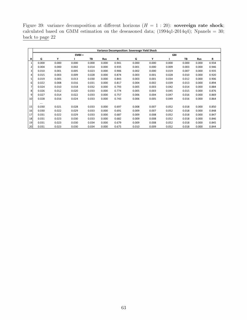
Figure 39: variance decomposition at different horizons (H = 1 : 20): sovereign rate shock;calculated based on GMM estimation on the deseasoned data; (1994q1-2014q4); Npanels = 30;back to page 22

H G Y I TB Rus R G Y I TB Rus R1 0.000 0.000 0.000 0.000 0.000 0.941 0.000 0.000 0.000 0.000 0.000 0.9342 0.004 0.000 0.002 0.014 0.000 0.935 0.001 0.000 0.009 0.003 0.000 0.9463 0.010 0.001 0.005 0.023 0.000 0.906 0.002 0.000 0.019 0.007 0.000 0.9354 0.015 0.003 0.009 0.028 0.000 0.874 0.003 0.001 0.028 0.010 0.000 0.9205 0.019 0.005 0.013 0.030 0.000 0.843 0.003 0.001 0.034 0.012 0.000 0.9066 0.022 0.008 0.016 0.031 0.000 0.817 0.004 0.002 0.039 0.013 0.000 0.8947 0.024 0.010 0.018 0.032 0.000 0.793 0.005 0.003 0.042 0.014 0.000 0.8848 0.026 0.012 0.020 0.033 0.000 0.774 0.005 0.003 0.045 0.015 0.000 0.8769 0.027 0.014 0.022 0.033 0.000 0.757 0.006 0.004 0.047 0.016 0.000 0.86910 0.028 0.016 0.024 0.033 0.000 0.743 0.006 0.005 0.049 0.016 0.000 0.864

….15 0.030 0.021 0.028 0.033 0.000 0.697 0.008 0.007 0.052 0.018 0.000 0.85016 0.030 0.022 0.029 0.033 0.000 0.691 0.009 0.007 0.052 0.018 0.000 0.84817 0.031 0.022 0.029 0.033 0.000 0.687 0.009 0.008 0.052 0.018 0.000 0.84718 0.031 0.023 0.030 0.033 0.000 0.682 0.009 0.008 0.052 0.018 0.000 0.84619 0.031 0.023 0.030 0.034 0.000 0.679 0.009 0.008 0.052 0.018 0.000 0.84520 0.031 0.023 0.030 0.034 0.000 0.675 0.010 0.009 0.052 0.018 0.000 0.844

VarianceDecomposition:SovereognYieldShockEMBI+ GBI

63

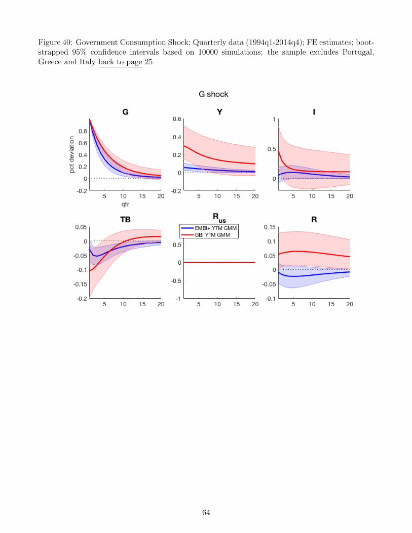
Figure 40: Government Consumption Shock; Quarterly data (1994q1-2014q4); FE estimates; boot-strapped 95% confidence intervals based on 10000 simulations; the sample excludes Portugal,Greece and Italy back to page 25

64

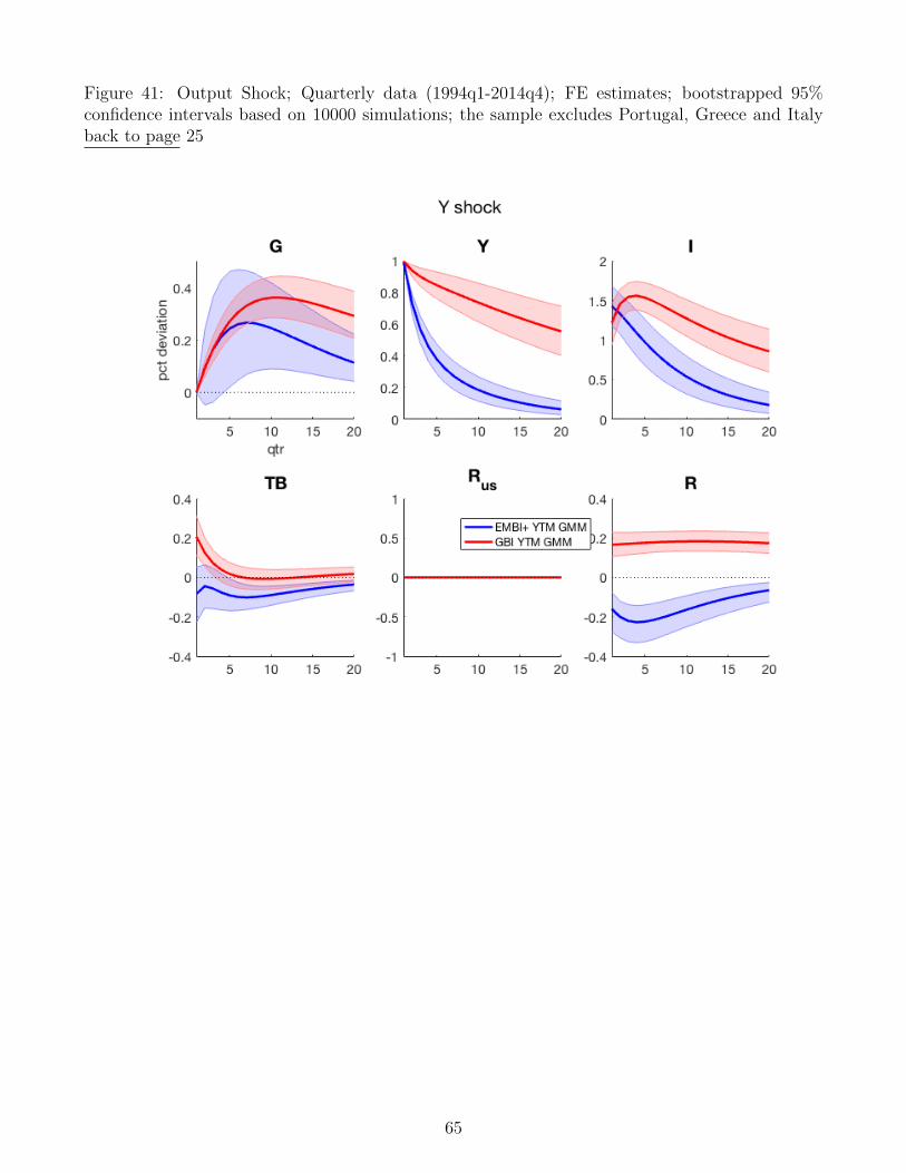
Figure 41: Output Shock; Quarterly data (1994q1-2014q4); FE estimates; bootstrapped 95%confidence intervals based on 10000 simulations; the sample excludes Portugal, Greece and Italyback to page 25

65

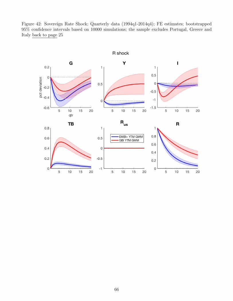
Figure 42: Sovereign Rate Shock; Quarterly data (1994q1-2014q4); FE estimates; bootstrapped95% confidence intervals based on 10000 simulations; the sample excludes Portugal, Greece andItaly back to page 25

66

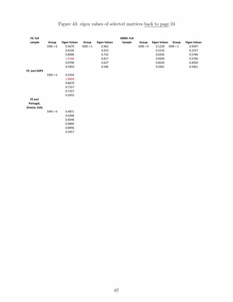
Figure 43: eigen values of selected matrices back to page 24

FE:fullsample Group EigenValues Group EigenValues

GMM:FullSample Group EigenValues Group EigenValues

EME=0 0.3670 EME=1 0.462 EME=0 0.1239 EME=1 0.93970.6234 0.915 0.2216 0.10170.8096 0.752 0.6426 0.57661.0106 0.817 0.9504 0.57660.9790 0.627 0.8534 0.49290.5959 0.596 0.5961 0.5961

FE:exclGIIPSEME=0 0.5559

1.00240.86700.71570.71570.5955

FEexclPortugal,

Greece,ItalyEME=0 0.4871

0.63060.85480.98940.89960.5957

67

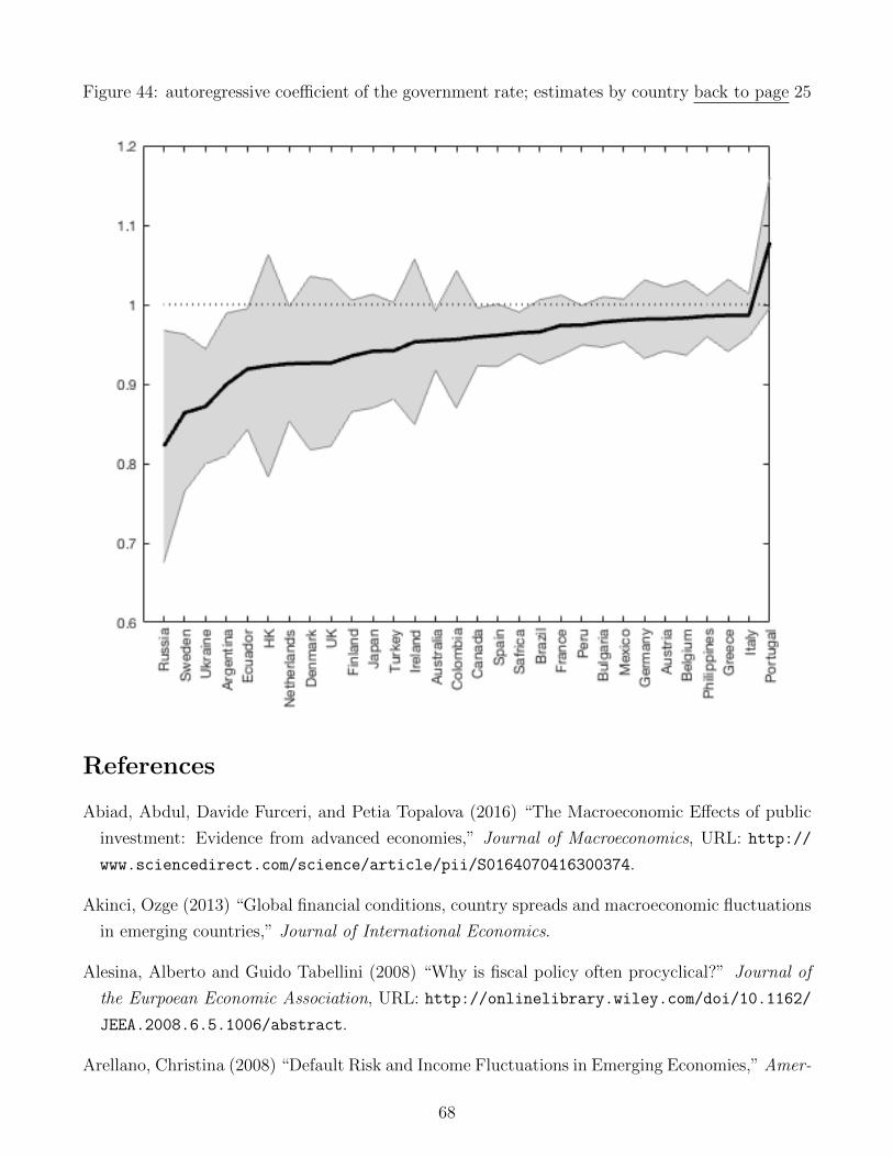
Figure 44: autoregressive coefficient of the government rate; estimates by country back to page 25

References

Abiad, Abdul, Davide Furceri, and Petia Topalova (2016) “The Macroeconomic Effects of public

investment: Evidence from advanced economies,” Journal of Macroeconomics, URL: http://

www.sciencedirect.com/science/article/pii/S0164070416300374.

Akinci, Ozge (2013) “Global financial conditions, country spreads and macroeconomic fluctuations

in emerging countries,” Journal of International Economics.

Alesina, Alberto and Guido Tabellini (2008) “Why is fiscal policy often procyclical?” Journal of

the Eurpoean Economic Association, URL: http://onlinelibrary.wiley.com/doi/10.1162/

JEEA.2008.6.5.1006/abstract.

Arellano, Christina (2008) “Default Risk and Income Fluctuations in Emerging Economies,” Amer-

68

ican Economics Review, URL: https://www.aeaweb.org/articles.php?doi=10.1257/aer.

98.3.690.

Arteta, Carlos and Galina Hale (2008) “Sovereign debt crises and credit to the private sector,”

Journal of International Economics, URL: http://ac.els-cdn.com/S0022199607000852/

1-s2.0-S0022199607000852-main.pdf?_tid=c850d660-480d-11e5-bba5-00000aab0f27&

acdnat=1440166153_fe310ac135c15f7a9e76b99e1e49d561.

Barro, Robert (1981) “Output Effects of Government Purchases,” Journal of Po-

litical Economy, URL: https://dash.harvard.edu/bitstream/handle/1/3451294/Barro_

OutputEffects.pdf?sequence=4.

Barro, Robert and Charles Redlick (2011) “Macroeconomic effect from government purchases and

taxes,” Quarterly Journal of Economics, URL: https://academic-oup-com.proxy.bc.edu/

qje/article/126/1/51/article.

Bi, Huixin (2012) “Sovereihn default risk premia, fiscal limits, and fiscal policy,” European Eco-

nomics Review.

Blanchard, Olivier and Roberto Perotti (2002) “An Empirical Characterization of the Dynamic

Effects of Changes in Government Spending and Taxes on Output,” The Quarterly Journal of

Economics.

Cuadra, Gabriel, Juan Sanches, and Horacio Sapriza (2010) “Fiscal policy and default risk in

emerging markters,” Review of Economic Dynamics, URL: http://www.sciencedirect.com/

science/article/pii/S1094202509000374.

Dawson, John and John Seater (2013) “Federal regulation and aggregate economic growth,” Jour-

nal of Economic Growth.

De Marco, Filippo (forthcoming) “Bank Lending and the European Sovereign Debt Crises,” Jour-

nal of Financial and Quantitative Analysis, URL: https://papers.ssrn.com/sol3/papers.

cfm?abstract_id=2673967.

Eichengreen, Barry and Ashoka Mody (1998) “What Explains Changing Spreads on Emerging-

Market Debt: Fundamentals or Market Sentiment?”, URL: https://ideas.repec.org/p/nbr/

nberwo/6408.html, NBER working paper.

Erten, Bilge (2012) “Macroeconomic transmission of Eurozone shocks to emerging economies,”

International Economics, URL: http://www.sciencedirect.com/science/article/pii/

S2110701713600542.

69

Fatas, Antonio and Ilian Mihov (2001) “The Effects of Fiscal Policy on Conspumption and Em-

ployment: Theory and Evidence,” CERP discussion paper.

(2003) “The Case for Restrictiong Fiscal Policy Discretion,” Quarterly Journal of Eco-

nomics, URL: http://faculty.insead.edu/ilian-mihov/documents/FPind.pdf.

Frankel, Jeffrey, Carlos Vegh, and Guillermo Vuletin (2012) “On Gradiation from Fiscal Pro-

cyclicality,” Journal of Development Economics, URL: https://wcfia.harvard.edu/files/

wcfia/files/jfrankel_graduation_fiscal_procyclicality.pdf.

Gali, Jordi, Lopez-Salido, and Javier Valles (2007) “Understanding the Effects of Government

Spending on Consumption,” Journal of European Economics, URL: http://www.nber.org/

papers/w11578.

Gavin, Michael and Roberto Perotti (1997) “Fiscal Policy in Larin America,” NBER Macroeco-

nomics Annual.

Hall, Robert (1986) The Role of Consumption in EconomicFluctuations: National Bureau of Eco-

nomic Research, URL: http://www.nber.org/chapters/c10024.pdf.

(2009) “By how much does GDP rise if the government buys more output?”, URL: http:

//www.nber.org/papers/w15496.pdf, working paper.

Ilzetzki, Ethan (2011) “Rent-seeking distortions and fiscal procyclicality,” Journal of

Development Economics, URL: http://ac.els-cdn.com/S0304387810000842/1-s2.

0-S0304387810000842-main.pdf?_tid=141cefa6-9783-11e5-8e90-00000aacb35f&acdnat=

1448902673_fb7fd7bd9adbed807bab32f970f95143.

Ilzetzki, Ethan, Enrique Mendoza, and Carlos Vegh (2013) “How big (small?) are fiscal mul-

tipliers?” Journal of Monetary Economics, URL: http://www.sciencedirect.com/science/

article/pii/S030439321200116X.

IMF (2014) Government Finance Statistics Manual, URL: https://www.imf.org/external/

Pubs/FT/GFS/Manual/2014/gfsfinal.pdf.

Jawadi, Fredj, Sushanta Mallick, and Ricardo Sousa (2016) “Fiscal and monetary policies in the

BRICS: A panel VAR approach,” Economic Modelling, URL: http://www.sciencedirect.

com/science/article/pii/S0264999315001455.

Kaminsky, Graciela, Carmen Reinhart, and Carlos Vegh (2004) “When it rains, it pours: procycli-

cal capital flows and macroeconomic policy,” September, URL: http://www.nber.org/papers/

w10780.pdf, NBER Working Paper.

70

Loayza, Norman, Anna Maria Oviedo, and Luis Serven (2004) “Regulation and Macroeconomic

Performance,” World Bank.

Lutkepohl, Helmut (2007) New Introduction to Multiple TIme Series Analysis: Springer.

McKay, Alisdair and Ricardo Reis (2016) “The Role of Automatic Stabilizers in the U.S. Business

Cycle,” Econometrica, URL: http://people.bu.edu/amckay/pdfs/autostab.pdf.

Mendoza, Enrique and P. Marcelo Oviedo (2006) “Fiscal Policy and Macroeconomic Uncertainty

in Developing Countries: The Take of the Tormented Insurer,” URL: http://www.nber.org/

papers/w12586.pdf, NBER working paper.

Mendoza, Enrique and Vivian Yue (2012) “A General Equilibrium Model of Sovereign Default and

Business Cycles,” The Quarterly Journal of Economics, URL: http://qje.oxfordjournals.

org/content/127/2/889.full.pdf+html.

Mertens, Karel and Morten Ravn (2011) “Understanding the aggregate ef-

fects of anticipated and unanaticipated tax policy shocks,” Review of Eco-

nomics Dynamics, URL: http://ac.els-cdn.com/S1094202510000359/1-s2.

0-S1094202510000359-main.pdf?_tid=9a8154d8-6b91-11e5-bae0-00000aacb35d&acdnat=

1444071061_d1d42dcd359d7cfc99772cda72851e0b.

Mountford, Andrew and Andrew Uhlig (2009) “What are the effects of fiscal policy

shocks?” Journal of Applied Econometrics, URL: https://ideas.repec.org/a/jae/japmet/

v24y2009i6p960-992.html.

Neumeyer, Pablo and Fabrizio Perri (2005) “Business cycles in emerging economies: the role

of interest rates,” Journal of Monetary Economics, URL: http://www.sciencedirect.com/

science/article/pii/S0304393205000036.

Perotti, Roberto (1999) “Fiscal Policy in Good Times and Bad,” The Quarterly Jour-

nal of Economics, URL: https://academic.oup.com/qje/article/114/4/1399/1934043/

Fiscal-Policy-in-Good-Times-and-Bad.

Raddatz, Claudio (2007) “Are external shocks responsible for the instability of output in low-

income countries?” Journal of Development Economics.

Ramey, Valerie (2011) “Identifying Geovernment Spending Shocks: It’s all in the Timimg,”

Quarterly Journal of Economics, URL: https://academic.oup.com/qje/article/126/1/1/

1902509/Identifying-Government-Spending-Shocks-It-s-all-in.

Riascos, Alvaro and Carlos Vegh (2003) “Procyclical Governement Spening in Developing Coun-

tries: the Role of Capital Market Imperfections,” October.

71

Romer, Christina and David Romer (2010) “The Macroeconomic Effects of Tax Changes: Es-

timates Based on a New Measure of Fiscal Shocks,” American Economic Review, URL:

https://www.aeaweb.org/articles?id=10.1257/aer.100.3.763.

Roodman, David (2009) “How to do xtabond2: An introduction to difference and system GMM

in Stata,” Stata Journal.

Rotemberg, Julio and Michael Woodford (1992) “Oligopolistic Pricing and the Effects of Aggregate

Demand on Economic Activity,” Journal of Political Economy, URL: http://www.jstor.org.

proxy.bc.edu/stable/pdf/2138830.pdf.

Sheremirov, Viacheslav and Sandra Spirovska (2017) “Outputresponse to government spending:

evidence from new international milirary spending data,” URL: https://www.fedinprint.org/

items/fedbwp/15-9.html, Fed in Print.

Talvi, Ernesto and Carlos Vegh (2005) “Tax Base Volatility and Pro-cyclical Fiscal Policy,” Journal

of Development Economics Economics, URL: http://www.mitpressjournals.org/doi/pdf/

10.1162/rest.91.4.850.

Uribe, Martin and Stephanie Schmitt-Grohe (2017) Open Economy Macroeconomics: Princeton

University Press, URL: http://press.princeton.edu/titles/11032.html.

Uribe, Martin and Vivian Yue (2006) “Country spreads and emerging economies,” Journal of

International Economics, URL: http://www.columbia.edu/~mu2166/uribe_yue_jie/uribe_

yue_jie.pdf.

Woo, Jaejoon (2009) “Why do more polarized countries run more procyclical fiscal policy?” The

Review of Economic Studies, URL: http://www.mitpressjournals.org/doi/abs/10.1162/

rest.91.4.850.

72