When does coordination pay?
17
Journal of Economic Dynamics and Control 14 (1990) 553-569. North-Holland WHEN DOES COORDINATION PAY?* Marcus MILLER and Mark SALMON Unkersity of Warwick, Cormtty CV4 7AL, Englad and CEPR Received January 1990 In a continuous-time model of two symmetric open economies, with a floating exchange rate, we find that the pay-off to macroeconomic policy coordination depends systematically on how heterogeneous is their inflation experience. While monetary policy coordination improves welfare in handling a common rate of underlying inflation, it exacerbates the ‘time consistency’ problem arising when there are differences (as is illustrated diagrammatically). Since the principle of ‘certainty equivalence’ applies to time-consistent policy in linear quadratic models, we are also able to give a stochastic interpretation of the deterministic results. 1. Introduction In a situation where monetary authorities are systematically targeting policy at a higher level of employment than wage setters, Rogoff (1985) showed that international coordination of monetary policy might not pay, as ‘inter-central bank cooperation can lead to systematically higher expected rates of inflation’. But, even when the target for policy is the natural rate itself, it may also be true that coordination is counterproductive, as we showed earlier in a continuous-time sluggish price ‘Dornbusch’ model of open economies with floating exchange rates; see the volume on ‘Interna- tional Economic Policy Coordination’ edited by Buiter and Marston (198.5). The appealing intuition that, by cooperating to internalise the externalities generated by monetary policy actions with floating rates, countries must necessarily be able to secure a welfare improvement, is evidently open to a form of Lucas critique: it ignores the impact that the act of coordinating itself can have on the expectations of market participants, and the constraints that this in turn will impose on policies which are jointly determined. Although the simulation results published in the same volume by Oudiz and Sachs (1985), using a similar model in discrete time, seemed to suggest *This paper was written as part of a research program on ‘Macroeconomic Interactions and Policy Design in an Interdependent World’, supported by grants from the Ford Foundation and the Alfred P. Sloan Foundation. Marcus Miller gratefully acknowledges the research funding supplied by the ESRC and research facilities provided by the NBER. 0165-1889/90/$3.50 8 1990, Elsevier Science Publishers B.V. (North-Holland)
-
Upload
marcus-miller -
Category
Documents
-
view
212 -
download
0
Transcript of When does coordination pay?

Journal of Economic Dynamics and Control 14 (1990) 553-569. North-Holland
WHEN DOES COORDINATION PAY?*
Marcus MILLER and Mark SALMON
Unkersity of Warwick, Cormtty CV4 7AL, Englad and CEPR
Received January 1990
In a continuous-time model of two symmetric open economies, with a floating exchange rate, we find that the pay-off to macroeconomic policy coordination depends systematically on how heterogeneous is their inflation experience. While monetary policy coordination improves welfare in handling a common rate of underlying inflation, it exacerbates the ‘time consistency’ problem arising when there are differences (as is illustrated diagrammatically). Since the principle of ‘certainty equivalence’ applies to time-consistent policy in linear quadratic models, we are also able to give a stochastic interpretation of the deterministic results.
1. Introduction
In a situation where monetary authorities are systematically targeting policy at a higher level of employment than wage setters, Rogoff (1985) showed that international coordination of monetary policy might not pay, as ‘inter-central bank cooperation can lead to systematically higher expected rates of inflation’. But, even when the target for policy is the natural rate itself, it may also be true that coordination is counterproductive, as we showed earlier in a continuous-time sluggish price ‘Dornbusch’ model of open economies with floating exchange rates; see the volume on ‘Interna- tional Economic Policy Coordination’ edited by Buiter and Marston (198.5). The appealing intuition that, by cooperating to internalise the externalities generated by monetary policy actions with floating rates, countries must necessarily be able to secure a welfare improvement, is evidently open to a form of Lucas critique: it ignores the impact that the act of coordinating itself can have on the expectations of market participants, and the constraints that this in turn will impose on policies which are jointly determined.
Although the simulation results published in the same volume by Oudiz and Sachs (1985), using a similar model in discrete time, seemed to suggest
*This paper was written as part of a research program on ‘Macroeconomic Interactions and Policy Design in an Interdependent World’, supported by grants from the Ford Foundation and the Alfred P. Sloan Foundation. Marcus Miller gratefully acknowledges the research funding supplied by the ESRC and research facilities provided by the NBER.
0165-1889/90/$3.50 8 1990, Elsevier Science Publishers B.V. (North-Holland)

554 M. Miller and M. Salmon, When does coordination pay?
that coordination must always pay, we show in this paper that the welfare conclusions from such two-country models are, in fact, sensitive to how different the initial inflationary conditions are in the two countries involved. In making these comparisons, we examine only ‘time-consistent’ policies, obtained using the technique discussed by Cohen and Michel(1988). It is well known that time-consistent policy may be welfare-inefficient [cf. Kydland and Prescott (1977)], and it appears that coordination will increase the potential for such inefficiency, at least when inflationary conditions differ between the two countries. The algebraic results are simply illustrated in a diagram - which also indicates the existence of simple rules which could (if they could be implemented) improve on ‘discretion’.
As the principle of certainty equivalence applies to time-consistent policies in such linear quadratic models, we are, following Levine and Currie (1987a), able to give a straightforward stochastic interpretation of our results, namely that coordination pays when supply-side (inflation) shocks are highly corre- lated, but may not when they are not.
Evidently, therefore, uncorrelated or negatively correlated inflation shocks pose a ‘time consistency problem’ which is exacerbated by coordination. There is, of course, a considerable literature on ‘solutions’ to this problem, so we conclude with some useful references and brief comments on policy implications.
2. Why coordination may fail
We consider a two-country version of sticky price, rational exchange rate model proposed by Dornbush (1976). The log-linear specification also in- cludes a term for core inflation to capture the effect of past inflation on current price setting; but there is no long-run trade-off between inflation and output. Even when policymakers are assumed to aim at a target of zero inflation at the ‘natural rate’ of output, there may nevertheless be ‘time consistency’ problems characterising the transition to such a noninflationary equilibrium.
A comparison is made between the optimal time-consistent policy chosen cooperatively and that which would result in a non-cooperative Nash equilib- rium. It is shown how the former will be welfare-improving where core inflation is initially the same in the two countries, but may fail otherwise. (The stochastic interpretation of these results is given in section 3 of the
paper.) The system of equations to be used is summarised in table 1; the specifica-
tion is, in fact, that of Miller and Salmon (1985a). The first pair indicates that real output is assumed to be ‘demand-determined’, where demand depends on local real interest rates, the real exchange rate, and output in the foreign country. (Asterisks are used to indicate variables pertaining to the foreign

Tab
le
1
A t
wo-
coun
try
mod
el.”
Hom
e co
untr
y
Agg
rega
te
dem
and
Phill
ips
curv
e
Cor
e in
flat
ion
Acc
umul
atio
n
Arb
itrag
e
y=
-yr+
Sc+q
y*
i=@
y+aD
c+v
rr=L
$$?i
&W
Dz=
y
E[D
c]
= r
- r*
Stat
ic
equa
tion
s
Dyn
amic
eq
uati
ons
Los
s fu
nctio
ns
min
V=
~llp
7r2+
y2
r I
Ham
ilto
nian
s
H =
;(p
r2
+y2
) +p
,Dz
+p,
*Dz*
“i
= ra
te
of c
hang
e of
co
nsum
er
pric
e in
dex,
in
flat
ion,
7r
= ‘
core
’ in
flat
ion,
y
= ou
tput
(i
n lo
gs)
mea
sure
d fr
om
the
natu
ral
rate
, z
= in
tegr
al
of
past
ou
tput
, c
= co
mpe
titiv
enes
s fo
r ho
me
coun
try
(in
logs
), i.e
., re
al
pric
e of
for
eign
go
ods,
r
= re
al
cons
umer
ra
te
of
inte
rest
, ps
= c
osta
te
(for
va
riab
le
s),
H=
H
amilt
onia
n,
E =
exp
ecta
tion
oper
ator
, D
E
diff
eren
tial
oper
ator
.
Ove
rsea
s co
untr
y
y* =
- y
r* +
6c +
7Jy
i*=+
y*-u
Dc-
r*
7T*
= &
Lz*
-
&rc
Dz*
=y
(4
)
(5)
min
V*=
I (6
) r*
2[
wL
??i*
?+y*
i
&
H”
= f(
p&
+y*
‘)+
p$D
z*
+p;
Dz
(7)
2 B
8 B
8 g.
3 Q
9 ‘W

556 M. Miller and A4. Salmon, When does coordination pay?
country.) The second pair of equations shows that the rate of change of Consumer Price Index in each country depends on local demand pressure, on ‘core’ inflation, and on the change in the real exchange rate (multiplied by (T, the share of imports in the price index).
Core inflation itself is defined in eq. (3) as the weighted sum of two components, whose evolution is shown in the two dynamic equations that follow. The first component, z, is a backward-looking variable, being the simple integral of past excess demand in the economy; see eq. (4). The second component, the real exchange rate, is taken to be a forward-looking variable: as indicated by eq. (.5), it is the integral of expected future interna- tional real interest rate differentials.
The stance of domestic monetary policy is characterised by the setting of the domestic real interest rate (Y or r*, respectively); and it is assumed that
policymakers aim to minimise the (undiscounted) integral of a quadratic function of excess demand and core inflation [see eq. (6)].
As there are three ‘state variables’, z, z*, and c, one can define the associated Hamiltonian functions, shown in eq. (7) as being the sum of the current contribution to the welfare loss plus the welfare cost of changes in the state variables. Note, however, that as we intend to examine only time-consistent policy, there is no explicit shadow cost for the real exchange rate. Instead, policymakers simply assume the real exchange rate depends linearly on the other state variables, where, by symmetry c = O(z - z*>, and 0 is determined to be ‘consistent’ with the resultant choice of policy [see Cohen and Michel (1988) and Miller and Salmon (1985bI1, as will be shown in fig. 1.
The results of policy optimisation can be calculated quite straightforwardly
for the case of coordinated policy where the instruments Y and r* (or equivalently, y and y*) are chosen so as to minimise the equally-weighted sum of I/ and V”, denoted by H” = (V+ V*)/2. The first-order conditions
are
(9)
where pt and p,“* denote the shadow prices that are associated with the

M. Miller and M. Salmon, When does coordination pay? 551
state variables z and z*, respectively. After some substitution, the dynamics
of the system of time-consistent coordinated policy chosen optimally can be represented by a fifth-order differential equation system (in z, z*, c, p7f, pf*>
as shown in panel A of table 2. Note that the parameter 0 must be determined as a function of the other parameters to ensure consistency.
Things are less straightforward for a Nash equilibtium. We note first, however, given the exchange rate is taken to be a linear function of state variables, that instead of setting Y and r* so as to minimise H and H*, respectively, we may alternatively set y and y* directly; i.e., one can treat output itself as the instrument. In a closed-loop no-memory Nash equilibrium each player allows for the feedback of the other’s policy rule on the current state variables, so the first-order conditions for the home country take the form:
dH -=y+pz=O, ay (12)
(13)
aH (14)
where it is assumed that y* =f2iz +fZ2zh and p, and pzs are the shadow prices associated with z and z* by the home policymaker. Similar equations can be obtained for the other country.
For analytical tractability, however, we make one last simplification here, namely to assume that the policymakers ignore each other’s feedback; in other words, we assume an open-loop Nash equilibrium.’ This is easier to characterise, as each player simply treats output elsewhere as predetermined and there is no need to define a shadow price for the state variable associated with it. Deleting the terms fi, and fz2 and the equation for Dp,, and combining this with the symmetric equations for the foreign country gives rise to the fifth-order system shown in table 2.
Comparing the coordinated and Nash equilibria is much simpler when these equation systems are partitioned in the manner recommended by Aoki (1981), namely by transforming the system, defining new variables as the averages of the original variables and also their differences. Since the
‘Notice that we employ the open-loop solution here solely in order to clarify the mathematical exposition of the argument. Referring back to our earlier results reported in the Buiter-Marston volume, we can see that whether coordination pays or not is not critically affected by whether we employ the open or closed-loop solution concepts.

558 M. Miller and M. Salmon, When does coordination pay?
Table 2
Optimal time-consistent policy.
I_
where
DZ Dz*
I 1 DC =
“P,
DP,*
(A) Coordinated policy
00 0 -2 0 Z
0 -2 Z*
0 2y-‘8 2y_‘(l+?7) -2y_‘(1+17) C
0 0 PE
0 0 II P,I* 1 : RI =g,= -(Psw)[(cfJ + d)* + (aq*], g* = gx = p.pdqq?J + c7
(B) Open-loop Nash
0 0 0 -1 0 0 0 0 0 -1
0 0 2y_‘6 yy’(1 + 7) -y-1(1 + 7)
-h(+ + ~0) hub’ 0 0 0
ha0 -h(4 +aB) 0 0 0
where h =p.$*($ +u0)
)
I Z z* c
P’r
PZ*
economies are symmetric, even regarding policy, this is an efficient form of diagonalisation of the original dynamics into two subsystems each involving one stable root. The consequences of doing so are given algebraically in table 3, with global averages in the left-hand column and international differences in the right-hand column.
(i) Global aueruges: With the aid of this table, we begin comparing the preferred policies for the system of averages, which is all that is relevant for disequilibria common to both countries. By construction, such disequilbria should not require any change in the level of competitiveness, c. Indeed, one finds that the relevant equations in the top left-hand corner of table 3, characterising coordinated policy, are just those of a closed economy, as no role is given to the exchange rate. Specifically, the determinant of the matrix
is P5 4~ , 2 2 but the trace is zero, so [A21 = p’/*[+; so the stable root is independent of the parameters (6, u, 0) reflecting the impact of the exchange rate.
This is not true, however, of the Nash equilibrium where it can be seen that [AtI= p’/25dm, so that the stable root depends on parameters relating to the exchange rate. Since, in the ‘differences’ case, to be examined next, 13 is typically negative and C#J + O(+ positive, this means that the system with policy being determined as a Nash equilibrium shows a slower response to such global disturbances than the cooperative case: comparing IAft with /A:[, we find that the term C$ is replaced by the geometric average of 4 and a term less than 4. Since, again by construction, there is no time inconsistency

M. Miller and M. Salmon, When does coordination pay? 559
Table 3
Time-consistent policy solutions (averages and differences).
Averages Differences
(A) Coordinated policy
DZ” [ I[ DP, =
: 2 ;2][;] [q-[-,:9., f$ 2(+][;] -Be 4 /2
(B) Open-loop Nash
[;;:I=[-“,& ;‘][;I [a]=[_% $2 v;;:lvy][;]
where h = pt2(4 + ~0) and h* = pt2(d + 2ofl) and 0 is to be determined.
problem arising for such common distrubances, such slowing down in speed of adjustment must be inefficient and hence increases welfare costs.
The explanation for the slower adjustment in the Nash equilibrium is that each policymaker, faced with excessive inflation, reckons that combatting inflation by setting high real interest rates will involve a temporary high real exchange rate (loss of competitiveness), and reasons furthermore that such an appreciation will have a direct beneficial effect on inflation via its impact on the CPI. Consequently, each national policymaker will relax somewhat the severity of his/her policy even though the real exchange rate must by symmetry remain unchanged in face of such common disturbances. It will be obvious to a policy coordinator that the (short-run) relief of exporting inflation via a high real exchange rate is not in fact open to either player: so coordinated policy is made more severe and inflation reduced faster.
By comparing the chosen policies, we thus find that coordination is more efficient for disequilibria common to both countries (and, by certainty equiva- lence, for perfectly correlated price shocks as we discuss further below). This welfare conclusion is the same as that of Oudiz and Sachs (1983 who also examined the case of common distrubances where the exchange rate need not adjust. But it does not necessarily carry over to the case of internationally differentiated disturbances as we now show.
(ii) Inter-country differences: Comparing policy choices in various strategic environments, given inter-country differences in state variables, is not quite so straightforward. The relevant dynamic equations are now third-order, as can be seen from the right-hand side of table 3. For convenience a graphical analysis will be used to study the relations between private-sector expecta- tions and policy choice (see fig. 11. These expectations are represented by the
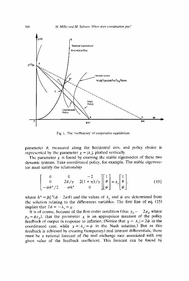
560 M. Miller and M. Salmon, When does coordination pay?
I/ I “Rational expectations’
lel=u+rlYw26/z)
/ \\I\ Nash ‘.
Fig. I. The ‘inefficiency’ of cooperative equilibrium.
parameter 8, measured along the horizontal axis, and policy choice is represented by the parameter A = [ASI, plotted vertically.
The parameter A is found by examing the stable eigenvector of these two dynamic systems. Take coordinated policy, for example. The stable eigenvec- tor must satisfy the relationship
0 0 -2 1 1
0 26/r 2(1+77)/y
-4h*/2 -ah* 0 III II 0 =A, f3 , (15)
* *
where h* = p~2(~ + 2~0) and the values of A, and 4 are determined from the solution relating to the differences variables. The first line of eq. (15) implies that 24 = -A, =A.
It is of course, because of the first-order condition (that y, = -2p, where pd = $z,>, that the parameter A is an appropriate measure of the policy feedback of output in response to inflation. (Notice that x = lAsl = 2r,!1 in the coordinated case, while x = lAsl = I) in the Nash solution.) But as this feedback is achieved by creating (temporary) real interest differentials, there must be a rational forecast of the real exchange rate associated with any given value of the feedback coefficient. This forecast can be found by

M. Miller and M. Salmon, When does coordination pay? 561
substituting A, = -x into the second line of (1.5) above and using x = 24
(for the coordinated case), i.e.,
2y-‘68 + r-‘( 1 + n)x = h,Ye = --x9,
to yield the explicit formula
PI = 1+17
y+ 26x-l. (16)
This is the ‘rational expectations’ relationship between the strength of policy response and exchange rate expectations which is common to both the Nash and coordinated solutions and is shown graphically by the schedule OR in the figure, which starts at the origin and rises to approach asymptotically a line (not shown) where 10 = ~~‘(1 + 7). The positive slope of the relation- ship indicates, as one would expect, that a stronger feedback response implies a greater movement in the forward-looking real exchange rate.
To find what value of feedback will actually be chosen with coordinated policymaking, we need to make use of the third relation implied in (15). After substitution for A,Y, as before, we obtain an explicit solution for x, namely
Xr = p”?$( 4 + 2aO). (17)
This relationship, showing how the choice of policy depends on private-sector expectations, is shown by the line ACB in the figure.
The time-consistent equilibrium for coordinated policy can now be found graphically as the intersection of the two curves OR and ACB, at the point labelled C in the figure. There, by construction, the private sector’s exchange rate expectations will be fulfilled and the policy coordinator is minimising welfare costs subject to such expectations.
A clearer picture of the nature of policy choice may be obtained by considering the iso-cost curves also shown in the figure, where these costs are measured by
#e*bP + 2d2 +A2 4A
G?(O) (18)
for inter-country differences. It is evident that the line ACB is a locus of points where
8W
ax 8 = 0, (19)
i.e., the feedback rules are chosen to minimise welfare costs subject to a time

562 M. Miller and M. Salmon, When does coordination pay?
consistency constraint that the parameter 13 be given, i.e., that expectations be a fixed (linear) function of the state variable [cf. Cohen and Michel (1988)l.
It is also clear that the time-consistent equilibrium is not efficient. The schedule OR must cross an iso-cost curve at point C, indicating that costs may be lowered by increasing the feedback coefficient. The point R*, where OR is tangent to an iso-cost curve, identifies that coefficient ,Y~*, which provides the best linear feedback rule, i.e., ‘the optimal rule’ referred to by Cohen and Michel. However, as such an equilibrium is not time-consistent, it would need to be sustained by threat strategies or involve some form of precommitment.
Finally, we consider what Nash behaviour implies for policy; the transition matrix relevant for this case is given in the lower right-hand panel of table 3. From these dynamic equations it is again evident that (given x = lA,l) rational expectations are represented by the schedule OR. However, the third rela- tion now implies the choice of greater feedback than coordinated policy. Specifically, we find
XN = p”2[\l( 4 + 2&)( 4 + ae>
i
4 + 2ui3 = *c 4+ue (20)
< xc over the range 0 < 0 < &.
The choice of feedback associated with Nash policy is shown in the dashed concave function ANB in the figure. Specifically, for any given value of 101, the Nash policy response is obtained as the geomettic acerage of the two values shown by the lines ACB and AF in the figure. Of course, so long as the Nash equilibrium, N, lies on an indifference curve of lower cost than that associated with point C, then ‘policy coordination does not pay’. [For the specific parameter values used in Miller and Salmon (1985a) for example (P=C=4=1,n=f,6=$, (T = O.l>, one finds that N lies between C and R*, as shown in the diagram.]
We have already noted that, given internationally differentiated inflation, time-consistent policy is not sufficiently rapid. The response of the exchange rate to policy choice (shown by OR) leads the coordinated policymaker to mitigate policy, since he/she perceives the temporary exchange rate adjust- ment to shift inflation from the high inflation to the negative inflation country, a most desirable development. Now it is also true that each of the national Nash policymakers is exposed to a similar temptation to mitigate feedback, as we have already seen; but the force of this is less as they do not
M. Miller and M. Salmon, When does coordination pay? 563
internalise the benefits of exporting inflation in bringing closer to zero inflation in the other country.
Specifically, we observe that the inflation equation applying to the coordi- nator (TV = [4zd + 25ac) is twice as sensitive to the exchange rate as that applying to each individual economy (e.g., 7 = .$4z + [cc). This is assumed to be apparent to participants in the foreign exchange market as well, so they will adjust their expectations accordingly. But these changed expectations will constrain the welfare improvements obtainable under time-consistent coordi- nation. Indeed the potential gains to coordination under floating rates may be negated by the increased inefficiency of time-consistent policy.
3. Coordination and correlation
In the previous section we have seen that, in a model where coordination must pay when both countries share the same initial inflationary position [so rr(0) = r*(O) = rO, 71;1= 01, it need not when they begin with differing rates of core inflation, and fig. 1 showed an example where moving to a Nash equilibrium could improve welfare. These results are reminiscent of those reported in Buiter and Marston (1985) where Oudiz and Sachs found that coordination of policy improved average welfare while we showed the con- trary.
What we do in this section is first of all to show that, in models of this kind, whether coordination pays or not depends on how big the arlerage core inflation in the initial conditions is compared with the discrepancy that exists between the two countries. (We calculate the critical ratio where coordina- tion has no welfare effect.) Second, using some results of Levine and Currie (1987a), we go on to provide a stochastic interpretation, namely that coordi- nation will tend to pay the more highly correlated are the supply-side shocks impinging on national inflation.
To do this it is convenient to disaggregate the total welfare cost into those elements contributed by average displacements and those associated with international differences, as follows:
=T ,cP(‘r2;““) + (qjdt
(21)

564 M. Miller and M. Salmon, When does coordination pay?
Table 4
Welfare weights for coordinated and Nash equilibria.”
Welfare
W
Weights Eigenvalues/vector
k, k, A, ‘d PI
Cooperative Open-loop Nash Closed-loop Nash
23.025 0.5000 0.10525 1.000 0.842 0.790 22.968 0.5001 0.1046X 0.981 0.896 0.825 22.970 0.5002 0.10465 0.972 0.888 0.820
where z:(O) = 25, z;(O) = 100
“From Buiter and Marston (1985, pp. 196, 200).
where X, and xd represent, respectively, the average (x +x*)/2 and differ- ences (x --x*1 of the variable X.
These integrals can be explicitly solved in terms of the stable roots A, and A, so
w= $(P7r:(o) +y,2(0)) - a
&pm +YxN (22)
= k,zf(O) + k2z,2(0) + k3Z2(0) + k&(O),
where k, and k, are the coefficients relating rrO and y, to z, and similarly for k, and k,. So we can write
W= k,z,2(0) + k&O), (23)
where k, and k, both depend on the parameters of the model and the strategic assumption characterising the setting of the policy.
In table 4, we show how the welfare costs obtained in our earlier study (see first column) can be obtained by summing the weighted initial displacements z:(O) and z;(O) using the weights shown in the next two columns. (The roots and the value of 19 obtained in each case are also shown, where of course optimisation was carried out subject to the time consistency condition that c = 8z,, with 0 being determined endogenously case by case.)
As can be seen from the table, k, is smaller with cooperation than without, while k, is larger with cooperation than in the Nash equilibria. As coopera- tion, in effect, reduces the weight applied to system-wide (average) displace- ments but increases the weight associated with differences, clearly the overall welfare payoff to coordination must depend on the relative sizes of the two

M. Miller and M. Salmon, When does coordination pay? 56.5
initial displacements. Indeed, by using (Y to denote their ratio, so (Y = z~(O)/z~(O), and by setting WcoOP = W Nash, or
k,Cz,Z(O) + k,Czj(O) = kfz,Z(O) + k,NzZ(O),
where kt, k$’ are the weights obtained from Nash equilibria and k,L’, k: are those associated with coordination, we can determine the critical point, LY*, where welfare costs are unaffected by whether policy is coordinated or not; namely
k,N-kk,C ff *=
k;-ky’
The reconciliation of the seemingly contradictory conclusions discussed earlier is now readily apparent. For, in models of this kind, coordination does not pay if the initial conditions are sufficiently disparate as between the countries involved, but it does when they are similar. In our 1985 study, we looked at the former case while Oudiz and Sachs considered the latter. (Specifically, in our study the parameter a, which represents the relative disparity was set at 4, well above its critical value, which turns out to be about 0.3 for closed-loop Nash equilibrium, as may be determined from table 4, while for Oudiz and Sachs both countries shared the same inflationary experience so cr is implicitly set at zero.) Hence the contrasting conclusions.
Now it may seem somewhat arbitrary that the payoff to coordination is determined by some historical ‘initial conditions’; but this simply reflects the deterministic nature of the analysis, where policymakers essentially only have to handle one disturbance (which is what the initial conditions describe). However, a paper published earlier in this journal by Paul Levine and David Currie (1987a), on the equivalence between deterministic welfare costs and the expected welfare costs arising from repeated stochastic shocks, provides a considerably more general interpretation of these results, which we now describe.
To make use of the equivalence which Levine and Currie establish, let random white-noise shocks affect the inflation equations. To ‘accommodate’ such supply-side shocks, eq. (2) is rewritten as
i dt = d(domestic price level) = 4y dt + 7~ dt + aE(dc) + db,
(2’) i*dt = d(foreign price level)
= 4y* dt + r* dt - aE(dc*) + db*,

566 M. Miller and M. Salmon, When does coordination pay?
where b and b* are Brownian motion processes characterised by an (instan- taneous) variance-covariance matrix
Note that these supply-side shocks are assumed to have the same variance in each country, and their correlation is denoted by the parameter p.
As a consequence, it is convenient to redefine the state variables (z, z*> to make them a summary of both demand and supply-side influences on inflation (where the latter are appropriately scaled); so eq. (4) becomes
dz=ydt+@-‘db and dz*=y*dt+4-‘db*. (4’)
To ensure time consistency one continues to impose the constraint that c = 13c.z -z*) when policy is being chosen. It is also necessary to introduce a discount factor, U, (common to both countries) into the (expected) cost function to ensure a finite expected loss, given by
E(V) = $Elm(@r( s)’ +y( S)2)e-“‘“-“ds, (6’)
and so too for V’*. To evaluate (asymptotic) expected costs from optimal time-consistent pol-
icy given such distrubances, one can appeal to Theorem 1 of Levine and Currie (1987a), which states ‘if the welfare (cost) of the deterministic prob- lem is written as W=f(Z(O)), then the corresponding welfare loss for the stochastic problem can be written as E(W) =~CU-’ Z)‘, where
Z(0) = [ 1 ;:(ybi, [z(O) z*(O) ] >
and C is a variance-covariance matrix of distrubances. What this result shows is that for a given initial displacement in a
deterministic context, one can find an appropriate correlation matrix for stochastic shocks which will generate the same (asymptotic, expected) cost. But, as the authors go on to show in Theorem 2, to obtain the expected costs of optimal (time-consistent) policy for a prespecified covariance matrix, one typically needs to sum up as many such ‘deterministic runs’ as there are uncorrelated shocks. In the present context, we find that the two determinis- tic runs correspond to the averages and differences simulations we have already examined, and that the ratio of the squared averages and differences is determined by the correlation coefficient, p.

M. Miller and M. Salmon, When does coordination pay? 567
To find the required deterministic runs (whose welfare costs will sum to the expected costs arising in the stochastic case), one diagonalises the (discounted) covariance matrix thus:
u-l~=u-l l p
[ 1 P 1
11 1 l+P 0 1 1 =----- 2z4 ] 1 -1 I[ 0 l-p I[ 1 -1 1
=(G)[$l 11+(%)[ Jl][l -11
= Z,(O) + Z,(O) *
But we note that the first deterministic data set corresponds to a matching displacement with z:(O) = (1 + p)/2u, and the second data has the displace- ment of opposite sign with zj(O) = 2(1 - p)/u. The ratio of the two is simply
4(O) 4(1 -P) -= zf(0) l-p ’
from which the stochastic interpretation of the two deterministic cases earlier discussed follows immediately. For, if as in Oudiz and Sachs, the initial values of the state variables are identical [so z:(O) = 01, then the welfare results obtained will match the asymptotic costs arising from perfktly corre- lated supply-side shocks (p = 1); but if, as for the simulations we reported in the Buiter-Marston volume, the ratio of squared initial conditions is 4 to 1, then the welfare results obtained will match the asymptotic costs arising from independent supply-side shocks (p = 0) - always provided that the determin- istic runs incorporate the discount factor, U, needed to obtain convergence in the stochastic case.’ Thus the theorems of Currie and Levine translate
*It must be noted, however, that the exact simulations reported in the Buiter-Marston volume are not precisely suited to our present purpose. Oudiz and Sachs incorporated a discount factor, but worked in discrete time: we worked in continuous time, but did no discounting. So in order, for example, to determine at what correlation of supply-side shocks the inefficiencies of time consistency are exactly balanced by gains of internal externalities, we would need to re-run the simulation including a discount factor to obtain cu*(u), and find the required correlation from setting (Y*(U) = 4(1 - p)/(l + p). We have not studied systematically how (Y* varies with U; but it would have to increase very sharply to avoid a conclusion that coordination will only pay if the shocks are highly correlated.

568 M. Miller and M. Salmon, When does coordination pay?
conclusions derived from particular initial conditions into results applying to specific patterns of repeated shocks - the generalisation promised earlier.
5. Policy implications and conclusions
The observation that coordination may not pay might be dismissed on the grounds that countries will, in that case, not choose to coordinate. This would, in our view, be a facile position to adopt, for two reasons. Firstly, because the setting of coordinated monetary policy is, in practice, likely to be part of a wider set of cooperative agreements (on trade, agricultural policy, defence, etc.), [see Currie et al. (1989)], so the welfare costs and benefits of monetary policy alone are unlikely to determine the overall decision of whether or not to cooperate. (We are grateful to K. Rogoff for this observa- tion.) Secondly, because the act of coordinating is likely to involve a substan- tial degree of commitment, it may not be very sensitive to small shifts in the covariance of stocks, which can nevertheless tip the balance of welfare advantage against coordination.
The problem cannot, therefore, simply be assumed away. One argument, which has been applied in a stochastic context, is that the consequences of reneging on private-sector expectations serves as a punishment, helping to sustain a wider class of coordinated policy rules [see, for example, Levine and Currie (1987b) and Levine, Currie, and Videlis (198711. But this argument depends crucially on the length and nature of the ‘punishment’ both of which are, to some degree, arbitrary. Instead, what we do, by way of conclusion, is to consider two obvious steps suggested by the preceding analysis to amelio- rate the situation. First we note that, since the possibility of welfare losses arises from the perceived ‘preferences’ of the policy coordinator, one might seek to ‘misrepresent’ these preferences. The appointment of a secretariat within the coordinating authority with views that are not simply an average of the countries concerned may achieve this effect.
We can see the effect of this ‘policy’ with reference to fig. 1, where the different slopes of the locus representing the policymaker’s feedback coeffi- cient under the Nash and coordinated assumptions determine for a given f3 the strength of policy response. Anything that can be done to increase the slope of the coordinator’s locus will produce a stronger monetary policy response. The coefficient p represents the weight attached to inflation in the policymaker’s cost function and, as can be seen, directly affects the slope of * = i/40) (i.e., - 2(~5p’/~>, so if the coordinator attaches a higher marginal cost to core inflation than the individual governments (misrepresenting his preferences), this may counteract the increase in the slope due to coordina- tion. Notice, however, that this option could be distinctly suboptimal if the shocks were symmetric rather than asymmetric.

M. Miller and M. Salmon, When does coordination pay? 569
This leads to the second alternative which is for the coordinator to discriminate between different types of shocks and to adopt a different fixed policy rule, i.e., ra = paz, and rd = pdzd in the face of these different shocks. As can be seen from fig. 1, there will be an optimal linear rule which dominates the time-consistent solutions, and the question then becomes one of achieving the credibility, by some means, of this optimal linear rule.
In this paper we have discussed how, in a simple two-country model, coordination may or may not pay depending on the correlation of distur- bances facing the two countries. The explanation for potential losses is that the benefits to cooperation be counteracted by the increased inefficiency of the time-consistent solution under cooperation. Since the welfare losses are simply those induced by the time inconsistency of optimal policy, many of the suggestions that already exist in the literature to ameliorate this problem may be applied in this situation; and we have briefly considered two alternatives.
References
Aoki, Masanao, 1981, Dynamic analysis of open economies (Academic Press, New York, NY). Cohen, Daniel and Phillippe Michel, 1988, How should control theory be used to calculate a
time consistent government policy?, Review of Economic Studies 55, 263-274. Currie, David, Gerry Holtham, and Andrew Hughes Hallet, 1989, The theory and practice of
international policy coordination: Does coordination pay?, in: Ralph, C. Bryant; David A. Currie, Jacob A. Frankel, Paul R. Masson, and Richard Portes, eds., Macroeconomic policies in an interdependent world (IMF, Washington, DC) 14-46.
Currie, David, Paul Levine, and Nit Vidalis, 1987, International cooperation and reputation in a empirical two-bloc model, in: Ralph C. Bryant and Richard Portes, eds.. Global macroeco- nomics: Policy conflict and cooperation (Macmillan, London) 75-12i.
Dornbusch, Rudiger, 1976, Expectations and exchange rate dynamics, Journal of Political Economy 84, 1161-I 176.
Kydland, Finn and Edward Prescott, 1977, Rules rather than discretion: The inconsistency of optimal plans, Journal of Political Economy 85, 473-491.
Levine, Paul and David Currie, 1987a, The design of feedback rules in linear stochatic rational expectations models, Journal of Economic Dynamics and Control 11, l-28.
Levine, Paul and David Currie. 1987b, Does international policy coordination pay and is it sustainable’? A two country analysis, Oxford Economic Papers 39, 38-74.
McKibben, Warwick J. and Jeffrey Sachs, 1986, Comparing the global performance of alternative exchange rate arrangements, Brookings discussion paper no. 49.
Miller, Marcus, 1985, Monetary stabilisation policy in an open economy, Scottish Journal of Political Economy 32, 220-233.
Miller, Marcus and Mark Salmon, 1985a, Policy coordination and dynamic games, in: Willem H. Buiter and Richard C. Marston, eds.. International economic policy coordination (Cambridge University Press. Cambridge) 184-213.
Miller, Marcus and Mark Salmon, 1985b, Dynamic games and the time inconsistency of optimal policy in open economies, Economic Journal (suppl.), 124-213.
Oudiz, Gilles and Jeffrey Sachs, 1985, International policy coordination in dynamic macroeco- nomic models, in: Willem H. Buiter and Richard C. Marston, eds., International economic policy coordination (Cambridge University Press, Cambridge) 274-319.
Rogoff, Kenneth, 1985, Can international monetary policy cooperation be counter-productive?, Journal of International Economics 18. 199-217.