1

When Banana Import Restrictions Lead to Exports:

A Tale of Cyclones and Quarantine Policies

Chia Chiun Ko and Paul Frijters

Abstract

This paper examines the welfare loss of import restrictions on bananas in Australia and

whether the import restrictions have turned into a particular form of export promotion. We set

up a model in which there is free domestic entry, with banana producers accepting losses in

normal years, off-set by large profits in years when cyclones destroy a large proportion of the

banana plants because of sufficiently low elasticity of demand. Using the cyclones of 2006

and 2011 as exogenous events, we identify the elasticity of demand for bananas in Australia

to be around -0.5. We indeed find limited evidence for an ‘over-shooting’ in terms of the

supply response after these cyclones, leading to positive exports years after cyclones have hit

and re-planted banana plants have become productive. Combining the elasticity estimates

with information on turnover, we get an estimated welfare loss of 600 million dollars per year

due to banana import restrictions.

Keywords: competition, import restrictions, exogenous shocks, instrumental variables,

surplus.

JEL classification: Q17, L2, C26, D61

2

Introduction

Krugman (1984) and Bhagwati (1988) explored the notion of export-promoting protection in

the context of particular market imperfections, such as monopolistic competition and

increasing returns to scale arising from industry linkages. The basic idea was that in the

presence of increasing returns to scale, initial import protection can lead an industry to grow

sufficiently such that domestic marginal costs become lower than world marginal costs,

leading to exports. This basic idea has subsequently been extended to allow for a role for

R&D and a variety of production linkages (eg. Pires, 2012, or Orladi and Gilbert, 2011).

In this paper we introduce a new mechanism for how import protection can lead to export-

promotion: supply shocks in agricultural production arising from natural disasters. In a very

simple model with free entry in the domestic market and complete import-restrictions, the

possibility of future supply shocks from natural disasters can lead to producers ‘betting’ on

those future natural disasters when demand is inelastic: despite the destruction of supply,

when demand is inelastic, profits are made just after disasters by those lucky not to have been

affected by the natural disaster, whilst in normal years producers will make losses. If demand

is sufficiently inelastic, the over-supply in normal years can be so large that the protected

industry exports despite marginal cost remaining above world levels at all times.

Our empirical example is the Australian banana industry, where complete import restrictions

have been in place since 19921. In 2006 and 2011, the main banana growing areas in the

North-East part of the country were hit by cyclones Larry and Yasi which destroyed large

parts of the banana plantations such that production dropped around 30% in both years. This

30% supply shock lead to a rise in banana retail prices from about 2 dollars a kilo prior to the

cyclones to 14 dollars a kilo just after the cyclones, leading to high profits amongst the

unaffected banana growers (Dixon 2011). The resulting post-cyclone long-term supply

reaction lead to a convergence with world prices and positive, though modest, exports in

2009 and 2010.

1 For an overview of papers and models used in the economics of banana production, see Blazy et al. (2011)

who study the willingness of farmers to adopt a variety of innovations in banana production in the Caribbean, an

area that is also susceptible to cyclones but where there are no banana import restrictions.

3

After setting up our simple model, we use the 2006 and 2011 cyclones to estimate the

demand elasticity for bananas, allowing us to calculate the welfare loss from banana import

restrictions. Since we have two cyclones, we can test for over-identification of our IV design.

The paper proceeds as follows: we first set up a simple theoretical model that explains the

mechanism from supply shocks to exports. We then give a brief background to the

institutions surrounding the banana industry in Australia, after which we explain our data. We

then run the analyses and show the implied welfare losses of import restrictions, followed by

conclusions.

The Model

We set up a standard two-period profit maximisation model, where production decisions are

taken in the first period and actual production and consumption takes place in the second

period, a delayed production assumption that particularly fits agriculture. In the second

period, domestic demand is given by , with the domestic price of bananas, where

, and The inverse function exists and is continuously decreasing, and will

be denoted as . Throughout we assume that the demand for bananas is inelastic,

meaning that

.

The total cost associated with the first period of a representative producer, who allocates

units of land to banana production is where is the marginal cost function and

. The increasing marginal cost reflects the standard argument that the first units of

land taken into production are the most appropriate. Again, the inverse of the marginal cost

function exists and is denoted as , which is presumed to exist and be continuously

decreasing.

In the second period, there is a probability of an adverse natural disaster that wipes out a

fraction of all cultivated banana land. The international banana market is now presumed to

consist of an infinite supply of bananas at world price ( ). As we are interested in the case

whereby the domestic market is not internationally competitive, we assume that

which implies that there would be positive imports without import restrictions.

So in a free-trade equilibrium; the price would be and would be

4

planted domestically. In the case of no natural disaster, domestic production in the second

period would be and foreign import would be . When there is

a natural disaster, domestic production in the second period would be , while

foreign imports would be .

Under the case of full import restrictions, the expected profit equation for the representative

banana grower is:

(1)

Where denotes total market production which in equilibrium will equal the level of

production of the representative grower. The first term indicates the amount of profits earned

when there is no natural disaster, while the second term indicates the amount of profits earned

when there is a natural disaster. The term incorporates the possibility that the

banana grower exports some of his production when the domestic price falls to the level of

the world price.

The equilibrium solution is then given by the first-order condition and the zero-profit

condition (using the fact that in equilibrium):

(2)

Where the presumed concavity of the cost-function ensures a unique market equilibrium. The

crucial question in this formulation is the circumstances under which the term

is negative, ie whether in times without a natural disaster a loss

is made because of the non-occurrence of the natural disaster. This turns out to follow

directly from the presumption of demand inelasticity: from demand inelasticity, we know

5

that

2. This in turn means must be smaller than in

the equation above; which together with the zero-profit condition implies that the first term

must be negative and the second term positive. Intuitively hence, banana growers expect to

make profits after a natural disaster and a loss in normal times. It immediately follows that if

demand of bananas is sufficiently inelastic (and the cost-function is sufficiently flat), then we

get the theoretical possibility that and that we thus get positive exports.

This very simple model also yields an expression for the welfare loss from an import ban on

the producer side. It simply consists of the costs of all banana production taking place above

world prices, and so is equal to . We can add this to the normal

deadweight loss that occurs on the consumer side to arrive at a total welfare loss.

Bananas: Institutions, Literature and Data

Bananas were originally introduced in Australia by Chinese migrants in the mid 19th

century.

After several ups and downs related to the disruptions of the world wars and world prices for

bananas and competing crops (such as sugar cane), the industry flourished after the 1960s.

The main variety of banana planted and marketed, both in Australia where it takes up about

80% of production and world-wide, is the Cavendish.

The industry was long characterised by some form of government protection and help, such

as particular railway lines facilitating transport built in the 1960s, and restrictive quarantine

regulations holding for foreign imports. By the 1990s, a total import ban for all foreign

bananas was in effect, with the official rationale being strict quarantine considerations, i.e.

that the import of bananas might aggravate the prevalence of banana diseases in Australia.

This rationale is subject of a WTO dispute between representatives of the Phillipino banana

growers on one hand and the Australian government on the other (see Javelosa and Schmitz

2006).

The economic literature on this in Australia has by and large been critical of these import

restrictions and its effects. An early contribution was by James and Anderson (1998), who

2 The proof for this expression is provided in the appendix.

6

undertook a simple economic assessment of the quarantine regulation. By comparing

domestic and world prices, they argued that consumer gains from lifting the import ban was

likely to outweigh the costs to banana producers, even in the extreme case of wiping out the

whole industry. There have also been earlier attempts at estimating the demand elasticity for

bananas in Australia, essentially using raw cross-sectional and time-series information,

finding elasticities in the range of -0.3 to -0.8 (Anderson and Stuckey 1974). A more recent

paper by Leroux and MacLaren (2011) also points to the deadweight loss of the import ban.

They run a more sophisticated bio-model that takes for granted that there is an Australian

natural interest in having a banana industry. They focus on the issue of diseases and advocate

a delayed lifting of the import ban, though gradually to allow for the development of local

defences to the spread of banana diseases. Yet, none of these contributions had exogenous

information to identify the demand elasticity with.

In terms of market characteristics, the Australian banana market fits the requirements of the

theoretical model: it is a very small producer in terms of the world market (around 0.003% of

world production), there are many banana producers in Australia (around 650 in 2012), and

there is a very large and competitive world market with somewhat stable prices in the whole

1990-2011 period (Evans and Ballen 2012). Furthermore, banana plants take at least 10

months to bear fruit, satisfying the condition of the model that the production decisions are

taken long before the supply uncertainty materialises and that there is no ability to increase

supply in the short run.

In terms of geographic spacing, bananas are grown in a fairly small region on the North-East

coast of Queensland where about 95% of all bananas grown in 2012 originated and that is

most suited in terms of climate for banana growing. Though there are some cross-state

restrictions in Australia, there are no effective entry or expansion restrictions for farmers

within the main banana growing area, or significant market concentration3.

Cyclones regularly affect this banana growing region, though different cyclones hit different

parts of that area. For instance, whilst cyclone Larry and Yasi both hit the main banana

growing areas, they were still several hundred kilometers apart in terms of their trajectories.

Similarly, an even bigger cyclone in 2006 (cyclone Monica) was too northerly to affect any

banana growing areas.

3 See Agricultural Commodities (Cat. no. 7121.0) published by Australian Bureau of Statistics

7

Basic Data

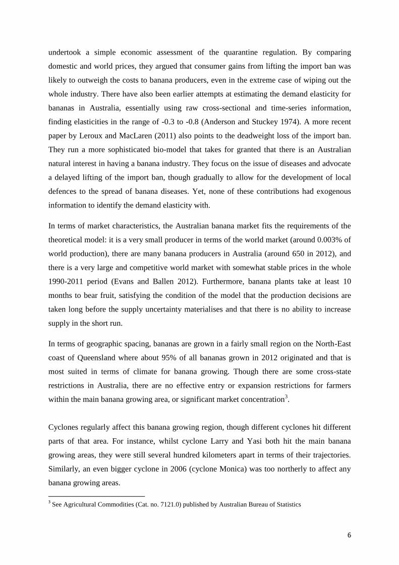
Figure 1, using data from the Australian Bureau of Statistics (ABS), shows the evolution of

banana production and the size of the banana growing area for the 1997-2012 period. It

shows how banana production slumped in 2006 and 2011, by roughly 30% each time,

following the cyclones. In terms of land used for banana production, we can see a steady

increase after 2006 and 2011 following the cyclones, perchance in reaction to the profits

made during the cyclone years.

Figure 1: Land Usage and Actual Production of Bananas in Australia

Figure 2 shows monthly domestic and world prices for Cavendish bananas after 2002. As one

can see, between 2002 and 2006 world and domestic prices were fairly close, but huge price

spikes were observed in the years of the cyclones, only returning back to ‘normal’ some 10

months after the cyclones, coinciding with the production delay of planting more bananas.

Most significantly, we can see a convergence in banana prices after the 2006 cyclone to

world price levels around 2009, as well as a return to world prices in July 2012.

8

Figure 2: Real Prices of Bananas- Australian and World Price

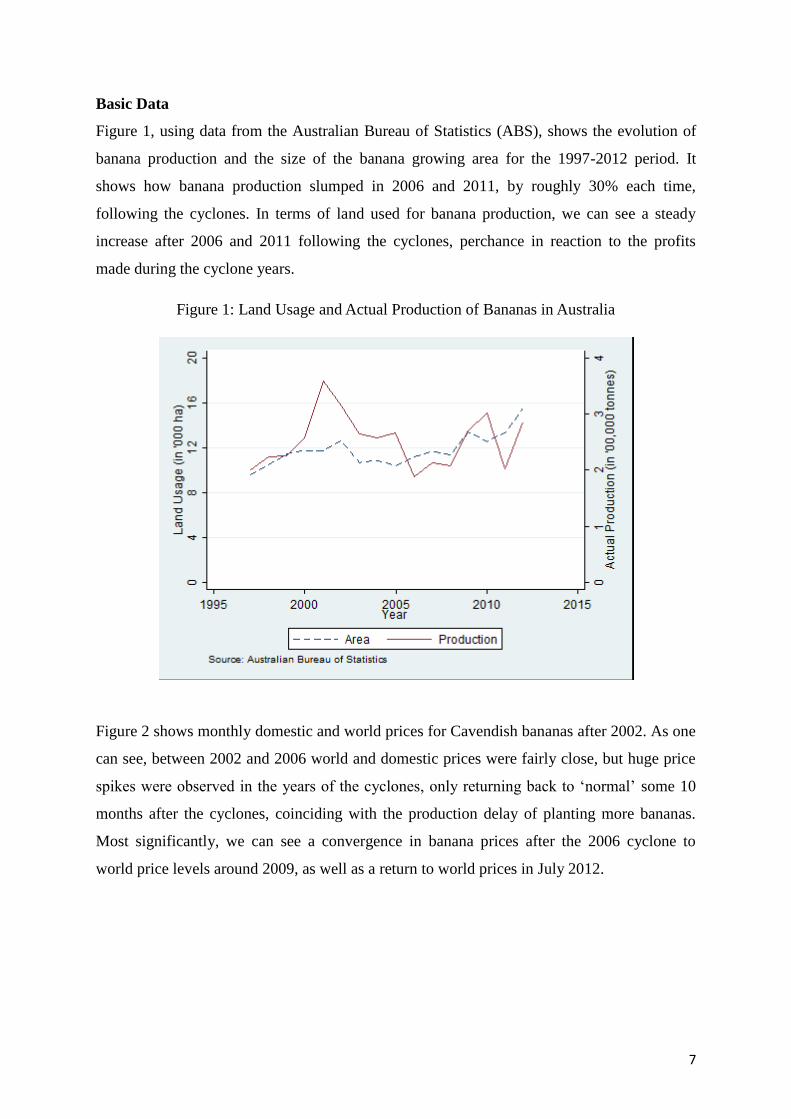
Figure 3 shows the exports of fresh bananas in these years, with significant positive export

levels in 2009 and 2010, dropping to zero in the years just after the cyclones. Considering the

increase in land where bananas are grown in recent years and the return to world prices, one

might expect significant banana exports again for 2013 and the ensuing years. We should also

say here though that fresh banana exports is not the only form of exports: whilst there is a

total import ban for fresh bananas, there are no import restrictions for many processed foods

that include bananas, such as muesli, fruit yogurts, soft-drinks, banana liqueur, etc. Hence the

effective ‘export margin’ is not only fresh-fruit export, but also import-substitution in the

processed food industry and the export of banana-derived processed foods (liqueur).

Unfortunately, the percentage of banana produced ending up in processed food is not well

documented, nor the origin of processed bananas in Australia, but processed bananas have

been estimated to be 35% of total banana production for the Philippines alone (SDCAsia

2006). With this in mind, the main indicator as to whether Australian bananas are effectively

traded on the margin on the world market is not the volume of fresh exports, but whether the

domestic price has converged with the international one. As one can see from Figure 2, this is

effectively the case for periods at least 2 years after the last cyclone.

0

2

4

6

8

10

12

14

16

Jan

-02

May

-02

Sep

-02

Jan

-03

May

-03

Sep

-03

Jan

-04

May

-04

Sep

-04

Jan

-05

May

-05

Sep

-05

Jan

-06

May

-06

Sep

-06

Jan

-07

May

-07

Sep

-07

Jan

-08

May

-08

Sep

-08

Jan

-09

May

-09

Sep

-09

Jan

-10

May

-10

Sep

-10

Jan

-11

May

-11

Sep

-11

Jan

-12

May

-12

Sep

-12

Pric

es

in $

/kg

Time (Monthly)

World Australia

(Source: Australian Bureau of Statistics)

9

Figure 3: Quantity of Banana Exports (in thousand kilograms)

Data used to estimate demand elasticities.

Bananas are traded on several wholesale markets in Australia, of which we have the monthly

data for the three biggest cities, Brisbane, Sydney and Melbourne, for the years 2002 to 2012.

Among these data, the Brisbane market is the only market that collects data on both the price

and quantity of bananas supplied, while data from the Sydney and Melbourne market only

contains the price of bananas supplied for every month.

Given these restrictions, the main demand analysis is done on the Brisbane market, though

we also will show results for all markets combined when we make the simplifying

assumption that the quantities traded on the markets are in constant proportions to the

Brisbane market, by using production data from the Agricultural Commodities (Cat. no.

7121.0) published by ABS.

Though there are many different types of bananas traded (Cavendish, Lady Finger, Red

Dacca, Goldfinger, Senorita and Ducasse), we will concentrate on the grade 1 Cavendish and

grade 1 Lady Finger bananas as they represent the vast bulk of production, with some 80% of

production being Cavendish bananas. In order to get real prices, we deflate by the Food

10

Component of the Consumer Price Index (CPI) for Australia published by ABS (Cat. no.

6401.0).

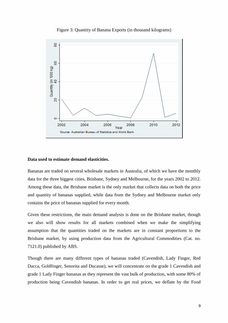
Estimation Strategy and Results

Our empirical supply equations relate the supply of bananas to prices, cyclones and other

variables:

log

(3)

Here equals the quantity of bananas supplied at time equals a vector of other

characteristics influencing supply (including lags of price and quantity traded and

general time trends); and are dummy variables indicating whether these

cyclones occurred in the last 9 months, corresponding to the lag in production response time;

and is a random variable. As this equation is in logs, we can directly interpret the

coefficients on Larry and Yasi as picking up the percentage of destroyed bananas in the

theoretical model (ρ), with the dependence on a first-order approximation of the

theoretical model with time-dependent cost and demand functions. The main estimation

variations are in terms of where we vary the lags in the prices and the time-periods

affected by the cyclones.

Our demand equation is then

(4)

Where is the quantity of bananas demanded at time Again, can include lags of the

price and trade. The main estimation problem is that there are good reasons to expect that the

error-term of this equation ( ) is related to the error term in the supply equation (

), for

instance because expectations of future price will influence both quantity supplied and price.

The main identifying assumption is then that the cyclone dummies are orthogonal to the error

terms and the other regressors, where the argument is that they are unanticipated shocks that

causally affect supply but not demand.

By equating demand to supply, we thus get the first-stage price estimation:

11

(5)

Where

and

and the instruments are exogenous to the composite error term

. Since will include effects from both the demand side of the market as well as

the supply side, the estimated will also include elements of both, meaning that its

coefficients have no straightforward natural interpretation. This simultaneous model is

estimated with GMM.

Results

The main results for the demand equations are in Table 1, with the results for the first-stage

price equations in the Appendix.

Table 1: Regression Results from Demand Equations

Brisbane Australia

(1) (2) (3) (4) (1) (2) (3) (4)

Variables

Price

-0.507*** -0.686*** -0.463***

-0.512*** -0.548* -0.348

(0.053) (0.216) (0.173)

(0.080) (0.307) (0.327)

Cavendish price

-0.396***

-0.325

(0.141)

(0.260)

last month's quantity

0.403** 0.213 0.207

0.715*** 0.672*** 0.665***

(0.203) (0.174) (0.174)

(0.147) (0.152) (0.153)

last month's price

0.440** 0.219 0.198

0.422 0.173 0.177

(0.177) (0.166) (0.154)

(0.308) (0.299) (0.272)

last year's average quantity

0.370*** 0.346**

-0.152 -0.157

(0.141) (0.142)

(0.755) (0.748)

last year's average price

0.315** 0.317***

-0.052 -0.060

(0.092) (0.093)

(0.147) (0.145)

Trend

0.097*** 0.093***

0.067 0.071

(0.034) (0.034)

(0.101) (0.101)

trend^2

-0.000*** -0.000***

-0.000 -0.000

(0.000) (0.000)

(0.000) (0.000)

Constant

13.983*** 8.297*** -21.551** -19.994** 17.404*** 4.938* -11.284 -12.398

(0.078) (2.868) (9.499) (9.434) (0.112) (2.598) (39.276) (39.051)

12

sample size 132 131 120 120 132 131 120 120

J-statistics 0.374 0.119 1.635 1.373 4.517 1.033 2.636 2.443

p-value of J-statistics 0.541 0.730 0.201 0.241 0.034 0.309 0.105 0.118

First stage Results

R-sq

0.743 0.830 0.841 0.817 0.761 0.832 0.852 0.828

F-statistics 147.700 17.261 20.967 21.768 130.67 17.073 22.748 23.061

Notes: F-statistics here is the joint significance of the instruments excluded from the structural model, which tests for weak

instruments. (1), (2), (3), (4) here denotes the four different kinds of specification for the model. Robust standard errors are shown in

the parentheses. *, ** and *** denote significance at 0.10, 0.05 and 0.01 levels.

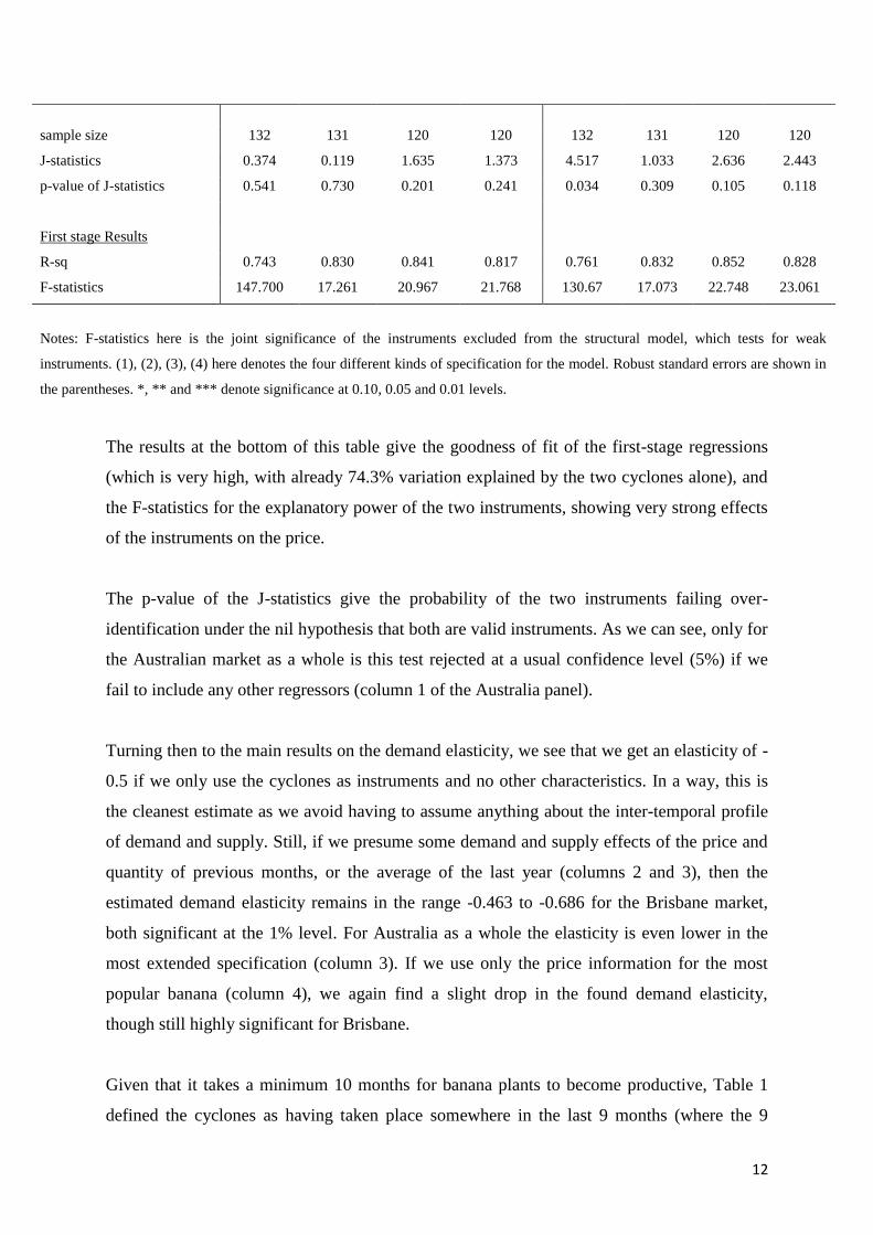
The results at the bottom of this table give the goodness of fit of the first-stage regressions

(which is very high, with already 74.3% variation explained by the two cyclones alone), and

the F-statistics for the explanatory power of the two instruments, showing very strong effects

of the instruments on the price.

The p-value of the J-statistics give the probability of the two instruments failing over-

identification under the nil hypothesis that both are valid instruments. As we can see, only for

the Australian market as a whole is this test rejected at a usual confidence level (5%) if we

fail to include any other regressors (column 1 of the Australia panel).

Turning then to the main results on the demand elasticity, we see that we get an elasticity of -

0.5 if we only use the cyclones as instruments and no other characteristics. In a way, this is

the cleanest estimate as we avoid having to assume anything about the inter-temporal profile

of demand and supply. Still, if we presume some demand and supply effects of the price and

quantity of previous months, or the average of the last year (columns 2 and 3), then the

estimated demand elasticity remains in the range -0.463 to -0.686 for the Brisbane market,

both significant at the 1% level. For Australia as a whole the elasticity is even lower in the

most extended specification (column 3). If we use only the price information for the most

popular banana (column 4), we again find a slight drop in the found demand elasticity,

though still highly significant for Brisbane.

Given that it takes a minimum 10 months for banana plants to become productive, Table 1

defined the cyclones as having taken place somewhere in the last 9 months (where the 9

13

months is taking the conservative approach). As a robustness exercise, we vary this window

from 7 months to 11 months, expecting the results from 7 months to be similar to those of 9

months but the results for 11 months to show much higher rates of elasticity as supply will

have reacted to the price shock following the cyclones.

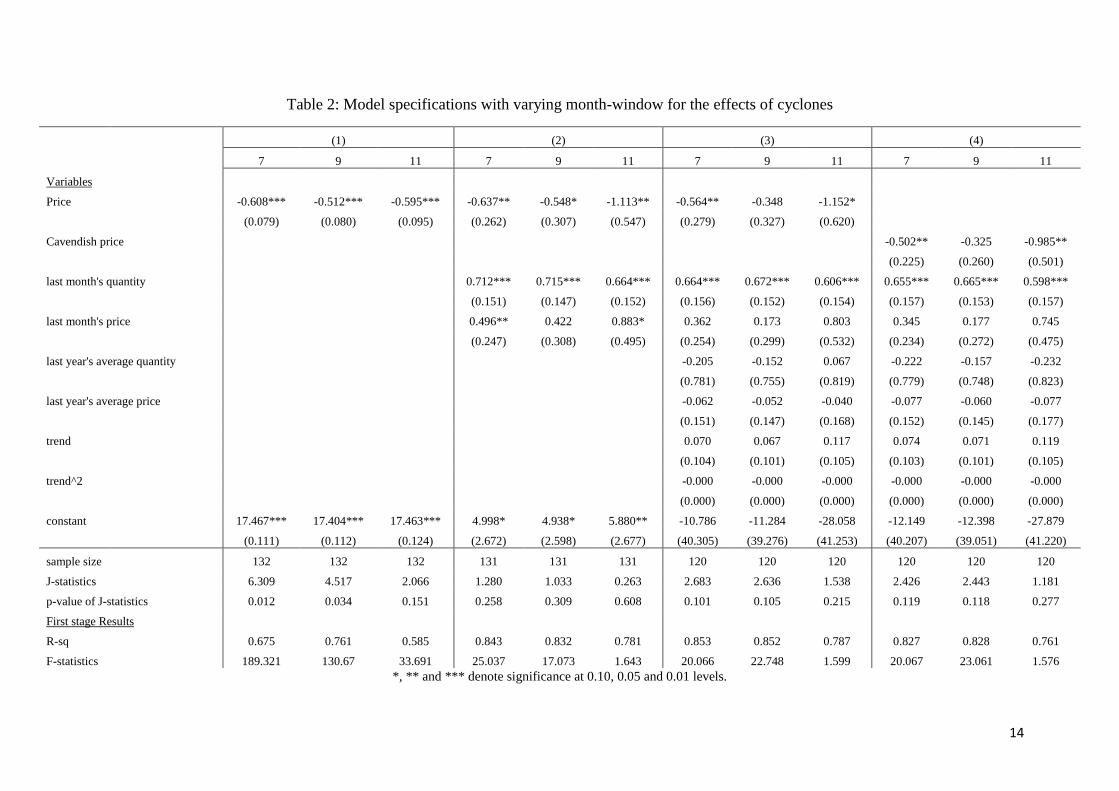
Table 2 shows these robustness exercises for the 4 main Australia-wide specifications, where

the 9 month specification always replicated the results for Australia in Table 1. As expected,

the difference between the estimated demand elasticities is small if we vary the Cyclone

window from 7 months to 9 months, with small decreases in the estimated elasticity when

increasing the window. Yet, when using an 11-month window there is a very strong increase

in estimated demand elasticities, even switching the main result in Specifications 2 and 3

from inelasticity (a coefficient higher than -1) to elasticity (a coefficient lower than -1). This

mainly shows the importance of endogeneity concerns with specifications lacking exogenous

variation.

14

Table 2: Model specifications with varying month-window for the effects of cyclones

*, ** and *** denote significance at 0.10, 0.05 and 0.01 levels.

(1) (2) (3) (4)

7 9 11 7 9 11 7 9 11 7 9 11

Variables

Price

-0.608*** -0.512*** -0.595*** -0.637** -0.548* -1.113** -0.564** -0.348 -1.152*

(0.079) (0.080) (0.095) (0.262) (0.307) (0.547) (0.279) (0.327) (0.620)

Cavendish price

-0.502** -0.325 -0.985**

(0.225) (0.260) (0.501)

last month's quantity

0.712*** 0.715*** 0.664*** 0.664*** 0.672*** 0.606*** 0.655*** 0.665*** 0.598***

(0.151) (0.147) (0.152) (0.156) (0.152) (0.154) (0.157) (0.153) (0.157)

last month's price

0.496** 0.422 0.883* 0.362 0.173 0.803 0.345 0.177 0.745

(0.247) (0.308) (0.495) (0.254) (0.299) (0.532) (0.234) (0.272) (0.475)

last year's average quantity

-0.205 -0.152 0.067 -0.222 -0.157 -0.232

(0.781) (0.755) (0.819) (0.779) (0.748) (0.823)

last year's average price

-0.062 -0.052 -0.040 -0.077 -0.060 -0.077

(0.151) (0.147) (0.168) (0.152) (0.145) (0.177)

trend

0.070 0.067 0.117 0.074 0.071 0.119

(0.104) (0.101) (0.105) (0.103) (0.101) (0.105)

trend^2

-0.000 -0.000 -0.000 -0.000 -0.000 -0.000

(0.000) (0.000) (0.000) (0.000) (0.000) (0.000)

constant

17.467*** 17.404*** 17.463*** 4.998* 4.938* 5.880** -10.786 -11.284 -28.058 -12.149 -12.398 -27.879

(0.111) (0.112) (0.124) (2.672) (2.598) (2.677) (40.305) (39.276) (41.253) (40.207) (39.051) (41.220)

sample size 132 132 132 131 131 131 120 120 120 120 120 120

J-statistics 6.309 4.517 2.066 1.280 1.033 0.263 2.683 2.636 1.538 2.426 2.443 1.181

p-value of J-statistics 0.012 0.034 0.151 0.258 0.309 0.608 0.101 0.105 0.215 0.119 0.118 0.277

First stage Results

R-sq 0.675 0.761 0.585 0.843 0.832 0.781 0.853 0.852 0.787 0.827 0.828 0.761

F-statistics 189.321 130.67 33.691 25.037 17.073 1.643 20.066 22.748 1.599 20.067 23.061 1.576

15

Another robustness exercise we did was to carry out bootstraps of the standard error with

asymptotic refinement on the t statistic, following Cameron and Travedi (2010). This did

increase the standard errors by roughly 20 percent, but did not change the qualitative result

that the estimated elasticities in specifications 1 and 2 are highly significant and well below

elastic. Results will be made available upon request.

Welfare calculations

We can now use our preferred demand elasticity estimate, which is the -0.5 for either

Brisbane or Australia when using only the cyclones and no other controls, to give a back-of-

the-envelope estimate of the welfare losses due to import restrictions.

As argued at the end of the theoretical model, there are two types of welfare losses: higher-

than-needed production costs and the deadweight loss of consumer surplus. These in fact

exist each period and are of different magnitudes each period due to the supply and demand

variations. Whilst we don’t have the information to directly estimate the cost-functions in the

theoretical model, we can appeal to the zero-profit condition to estimate the loss at the

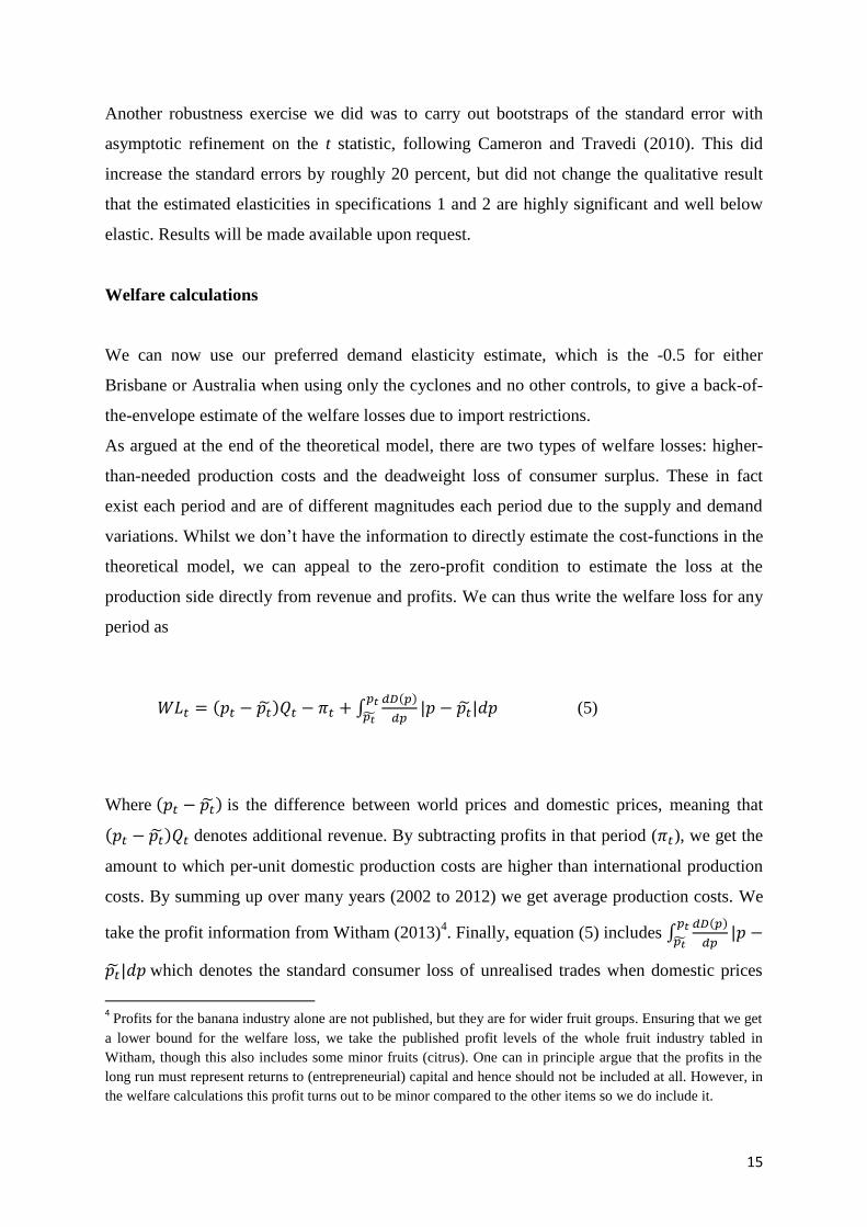
production side directly from revenue and profits. We can thus write the welfare loss for any

period as

(5)

Where is the difference between world prices and domestic prices, meaning that

denotes additional revenue. By subtracting profits in that period ( ), we get the

amount to which per-unit domestic production costs are higher than international production

costs. By summing up over many years (2002 to 2012) we get average production costs. We

take the profit information from Witham (2013)4. Finally, equation (5) includes

which denotes the standard consumer loss of unrealised trades when domestic prices

4 Profits for the banana industry alone are not published, but they are for wider fruit groups. Ensuring that we get

a lower bound for the welfare loss, we take the published profit levels of the whole fruit industry tabled in

Witham, though this also includes some minor fruits (citrus). One can in principle argue that the profits in the

long run must represent returns to (entrepreneurial) capital and hence should not be included at all. However, in

the welfare calculations this profit turns out to be minor compared to the other items so we do include it.

16

are different from world prices, for which we use the estimated equation (4). The use of the

absolute price differential, , reflects the fact that when the domestic price is above

world price the consumer loss is driven by an inability to buy from the world market, whereas

if it is below the world price the consumer loss is driven by an inability to sell to the world

market.

We can estimate the first part of this equation using our price data and the volume of trades

for Australia in the 2002-2012 period. We need to show this for the whole period though,

since we will be adding up years of profit with years of losses. We can estimate the second

part using our favoured estimate for demand elasticity from Table 2, ie -0.5. Table 3 shows

these estimated welfare losses coming from the producer side.

17

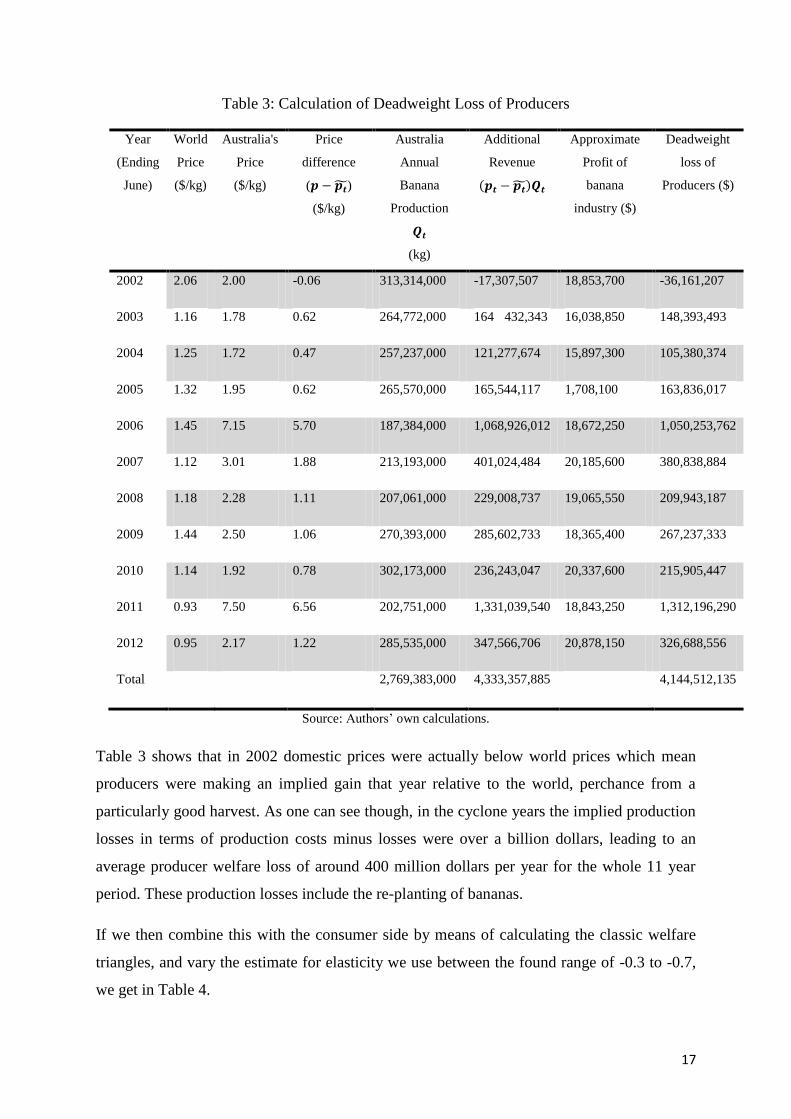
Table 3: Calculation of Deadweight Loss of Producers

Year

(Ending

June)

World

Price

($/kg)

Australia's

Price

($/kg)

Price

difference

( )

($/kg)

Australia

Annual

Banana

Production

(kg)

Additional

Revenue

Approximate

Profit of

banana

industry ($)

Deadweight

loss of

Producers ($)

2002 2.06 2.00 -0.06 313,314,000 -17,307,507 18,853,700 -36,161,207

2003 1.16 1.78 0.62 264,772,000 164 432,343 16,038,850 148,393,493

2004 1.25 1.72 0.47 257,237,000 121,277,674 15,897,300 105,380,374

2005 1.32 1.95 0.62 265,570,000 165,544,117 1,708,100 163,836,017

2006 1.45 7.15 5.70 187,384,000 1,068,926,012 18,672,250 1,050,253,762

2007 1.12 3.01 1.88 213,193,000 401,024,484 20,185,600 380,838,884

2008 1.18 2.28 1.11 207,061,000 229,008,737 19,065,550 209,943,187

2009 1.44 2.50 1.06 270,393,000 285,602,733 18,365,400 267,237,333

2010 1.14 1.92 0.78 302,173,000 236,243,047 20,337,600 215,905,447

2011 0.93 7.50 6.56 202,751,000 1,331,039,540 18,843,250 1,312,196,290

2012 0.95 2.17 1.22 285,535,000 347,566,706 20,878,150 326,688,556

Total 2,769,383,000 4,333,357,885 4,144,512,135

Source: Authors’ own calculations.

Table 3 shows that in 2002 domestic prices were actually below world prices which mean

producers were making an implied gain that year relative to the world, perchance from a

particularly good harvest. As one can see though, in the cyclone years the implied production

losses in terms of production costs minus losses were over a billion dollars, leading to an

average producer welfare loss of around 400 million dollars per year for the whole 11 year

period. These production losses include the re-planting of bananas.

If we then combine this with the consumer side by means of calculating the classic welfare

triangles, and vary the estimate for elasticity we use between the found range of -0.3 to -0.7,

we get in Table 4.

18

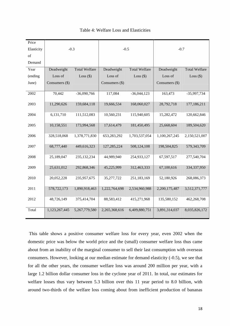
Table 4: Welfare Loss and Elasticities

Price

Elasticity

of

Demand

-0.3

-0.5

-0.7

Year

(ending

June)

Deadweight

Loss of

Consumers ($)

Total Welfare

Loss ($)

Deadweight

Loss of

Consumers ($)

Total Welfare

Loss ($)

Deadweight

Loss of

Consumers ($)

Total Welfare

Loss ($)

2002 70,442 -36,090,766 117,084 -36,044,123 163,473 -35,997,734

2003 11,290,626 159,684,118 19,666,534 168,060,027 28,792,718 177,186,211

2004 6,131,710 111,512,083 10,560,231 115,940,605 15,282,472 120,662,846

2005 10,158,551 173,994,568 17,614,479 181,450,495 25,668,604 189,504,620

2006 328,518,068 1,378,771,830 653,283,292 1,703,537,054 1,100,267,245 2,150,521,007

2007 68,777,440 449,616,323 127,285,224 508,124,108 198,504,825 579,343,709

2008 25,189,047 235,132,234 44,989,940 254,933,127 67,597,517 277,540,704

2009 25,631,012 292,868,346 45,225,999 312,463,333 67,100,616 334,337,950

2010 20,052,228 235,957,675 35,277,722 251,183,169 52,180,926 268,086,373

2011 578,722,173 1,890,918,463 1,222,764,698 2,534,960,988 2,200,175,487 3,512,371,777

2012 48,726,149 375,414,704 88,583,412 415,271,968 135,580,152 462,268,708

Total 1,123,267,445 5,267,779,580 2,265,368,616 6,409,880,751 3,891,314,037 8,035,826,172

This table shows a positive consumer welfare loss for every year, even 2002 when the

domestic price was below the world price and the (small) consumer welfare loss thus came

about from an inability of the marginal consumer to sell their last consumption with overseas

consumers. However, looking at our median estimate for demand elasticity (-0.5), we see that

for all the other years, the consumer welfare loss was around 200 million per year, with a

large 1.2 billion dollar consumer loss in the cyclone year of 2011. In total, our estimates for

welfare losses thus vary between 5.3 billion over this 11 year period to 8.0 billion, with

around two-thirds of the welfare loss coming about from inefficient production of bananas

19

and one-third in terms of consumer loss. Total reported profits in this period are only around

230 million, meaning that subtracting them or not changes no more than 5% of this headline

figure at most.

Discussion

This paper introduced a new mechanism for the circumstances in which import restrictions

can lead to exports, focusing on the role of supply shocks due to natural disasters when

demand is inelastic and supply responses are sluggish due to lags between investments and

production. It was argued that the supply shocks created the possibility that suppliers would

‘bet’ on a negative supply shock when they would make, in expectation, a profit, leading to

over-supply in periods in which the negative supply shock did not eventuate.

The empirical section then looked at the Australian banana industry, arguing that the price

increase in years when cyclones wiped out 30 percent of production was sufficiently high to

generate an increase in subsequent production capacity and actual exports several years after

the cyclones. Using the cyclones as unanticipated exogenous shocks, we found a demand

elasticity of around -0.5, leading to an estimated yearly welfare loss of some 600 million

dollars a year due to the import restrictions, of which around two-thirds comes from

inefficient production and one third from loss of consumer surplus. This is more than twice as

high as total revenue in normal years, driven by large losses on both the producer and

consumer surplus sides in cyclone years. In effect, each banana producer, of which there are

around 600, gets a subsidy worth a million dollars each year. It is a fairly extreme example of

import protection and with such a subsidy it is perhaps not surprising that it might lead to

exports.

If we reflect on it, the mechanism for import-protection driven export-promotion unearthed in

this paper would seem to be a niche mechanism that is unlikely to hold for many industries

and that is hence mainly an economic curiosum. Not only would an industry need a long

lead-time in terms of production to fit this model, but it would also have to be the case that

there is no relatively cheap way to avoid the negative exogenous shock that is responsible for

the supply shocks. That in turn would seem to limit the mechanism to primary products that

are highly dependent on a very specific eco-system that is not replicable elsewhere within the

protected market. And the products made in that eco-system would furthermore need to

20

supply a relatively inelastic consumer market and nevertheless be a world commodity (so not

too tied to a single eco-system either). All we can think of is a set of tropical fruits

(pineapple, coconuts, dates) that are subject to storms and diseases, particular primary niche-

products that depend on a limited number of areas and are subject to disease and climate

(such as truffles depending on particular types of forest) and animals-bred-in-captivity where

total supply is subject to the uncertainties of poaching and disease (lions and tigers). For

those types of markets, import restrictions could lead to the curious and expensive

phenomenon of loss-making exports.

On the other hand, natural disasters are a frequent occurrence in many areas and there may be

other investment and production situations giving rise to other yet unexplored economic

curiosa.

21

References

Anderson, JR & Stuckey, JA 1974, ‘Demand Analysis of the Sydney Banana Market’, Review of

Marketing and Agricultural Economics Society, Australian Agricultural and Resource Economics

Society, vol. 42, no. 1, pp. 56-69.

Australian Bureau of Statistics 2013, Agricultural Commodities, Australia, 2011-2012, Cat. no.

7121.0, Australian Bureau of Statistics, http://www.abs.gov.au/ausstats/abs@.nsf/mf/7121.0.

Australian Bureau of Statistics 2013, Consumer Price Index, Australia, Mar 2013, Cat. no. 6401.0,

ABS, http://www.abs.gov.au/AUSSTATS/abs@.nsf/DetailsPage/6401.0Jun%202011.

Australian Bureau of Statistics 2013, Australian Demographic Statistics, Mar 2013, Cat. no. 3101.0,

Australian Bureau of Statistics, Canberra, http://www.abs.gov.au/AUSSTATS/abs@.nsf/mf/3101.0.

Bhagwati, J 1988, ‘Export-promoting Protection: Endogenous Monopoly and Price Disparity’, The

Pakistan Development Review, vol. 27, no. 1, pp. 1-5.

Blazy, J. M., Carpentier, A., & Thomas, A. (2011). The willingness to adopt agro-ecological

innovations: Application of choice modelling to Caribbean banana planters. Ecological Economics,

72, 140-150.

Cameron, AC & Trivedi, PK 2010, Microeconometrics Using Stata, Revised Edition, Stata Press,

Texas

Evans, E & Ballen, F 2012, Banana Market, University of Florida IFAS Extension, viewed 20

September 2013, < http://edis.ifas.ufl.edu/fe901>.

Javelosa, J & Schmitz, A 2006, ‘Costs and Benefits of a WTO Dispute: Philippine Bananas and the

Australian Market’, Estey Centre Journal of International Law and Trade Policy, 7, pp. 58-83.

Krugman, PR 1984, ‘Import Protection as Export Promotion: International Competition in the

Presence of Oligopoly and Economies of Scale’, in Krugman PR (1990), Rethinking International

Trade, The MIT Press, Massachusetts, pp. 185-198.

Leroux, A & Maclaren, D 2011, ‘The Optimal Time to Remove Quarantine Bans under Uncertainty:

The Case of Australian Bananas’, Economic Record, 87, pp. 140-152.

Market Information Services 2013, Brisbane Monthly Bananas, Market Information Services,

Brisbane, Unpublished Historical Dataset.

22

Market Information Services 2013, Melbourne Annual Bananas, Market Information Services,

Brisbane, Unpublished Historical Dataset.

Market Information Services 2013, Sydney Annual Bananas, Market Information Services, Brisbane,

Unpublished Historical Dataset.

Oladi, R., & Gilbert, J. (2011). Monopolistic Competition and North–South Trade. Review of

International Economics, 19(3), 459-474. North-South, monopolistic competition.

Pires, A. J. G. (2012). International trade and competitiveness. Economic Theory, 50(3), 727-763.

Pires, A. J. G. (2012). Home market effects with endogenous costs of production. Journal of Urban

Economics.

23

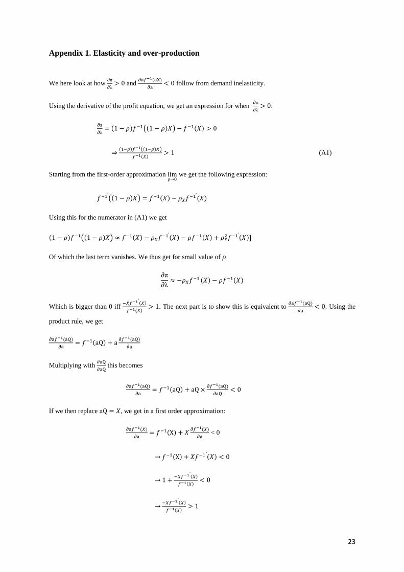
Appendix 1. Elasticity and over-production

We here look at how

and

follow from demand inelasticity.

Using the derivative of the profit equation, we get an expression for when

:

(A1)

Starting from the first-order approximation ρ

we get the following expression:

Using this for the numerator in (A1) we get

Of which the last term vanishes. We thus get for small value of

Which is bigger than 0 iff

. The next part is to show this is equivalent to

. Using the

product rule, we get

Multiplying with

this becomes

If we then replace , we get in a first order approximation:

< 0

24

Which is the desired expression. By iteration, the same equivalence also goes for higher values of

Appendix 2: Supply equations.

Table A1: First Stage Supply Results

Brisbane Australia

First stage Results (1) (2) (3) (4) (1) (2) (3) (4)

Larry

1.508*** 0.795*** 0.980*** 1.185*** 1.398*** 0.757*** 0.888*** 1.072***

(0.131) (0.135) (0.140) (0.167) (0.113) (0.131) (0.138) (0.164)

Yasi

1.590*** 0.757*** 1.077*** 1.241*** 1.279*** 0.666*** 1.004*** 1.153***

(0.119) (0.177) (0.211) (0.248) (0.117) (0.153) (0.190) (0.228)

last month's quantity

-0.062 -0.113** -0.139**

-0.025 -0.042 -0.054

(0.037) (0.050) (0.060)

(0.026) (0.027) (0.034)

last month's price

0.496*** 0.355*** 0.351***

0.476*** 0.360*** 0.351***

(0.072) (0.076) (0.092)

(0.074) (0.077) (0.095)

last year's average quantity

0.150* 0.124

-0.278 -0.339

(0.084) (0.115)

(0.310) (0.397)

last year's average price

0.203** 0.235**

0.057 0.039

(0.086) (0.108)

(0.097) (0.126)

Trend

0.090*** 0.093***

0.042 0.052

(0.029) (0.035)

(0.031) (0.040)

trend^2

-0.000*** -0.000**

-0.000 -0.000

(0.000) (0.000)

(0.000) (0.000)

Constant

0.662*** 1.168*** -26.036*** -26.378*** 0.560*** 0.712 -5.730 -8.543

(0.029) (0.506) (8.315) (9.843) (0.023) (0.436) (12.933) (16.673)

sample size 132 131 120 120 132 131 120 120

R-sq

0.743 0.830 0.855 0.828 0.761 0.832 0.853 0.828

F-statistics 147.700 197.900 109.550 103.69 130.670 147.640 77.20 75.11

Notes: F-statistics here is the joint significance of all variables. (1), (2), (3), (4) here denotes the four different

kinds of specification for the model. Robust standard errors are shown in the parentheses. *, ** and *** denote

significance at 0.10, 0.05 and 0.01 levels.