
What's News in Business Cycles - Columbia University in ...mu2166/news_in_bc/paper.pdf · WHAT’S...
33
http://www.econometricsociety.org/ Econometrica, Vol. 80, No. 6 (November, 2012), 2733–2764 WHAT’S NEWS IN BUSINESS CYCLES STEPHANIE SCHMITT -GROHÉ Columbia University, New York, NY 10027, U.S.A., CEPR, and NBER MARTÍN URIBE Columbia University, New York, NY 10027, U.S.A. and NBER The copyright to this Article is held by the Econometric Society. It may be downloaded, printed and reproduced only for educational or research purposes, including use in course packs. No downloading or copying may be done for any commercial purpose without the explicit permission of the Econometric Society. For such commercial purposes contact the Office of the Econometric Society (contact information may be found at the website http://www.econometricsociety.org or in the back cover of Econometrica). This statement must be included on all copies of this Article that are made available electronically or in any other format.
Transcript of What's News in Business Cycles - Columbia University in ...mu2166/news_in_bc/paper.pdf · WHAT’S...
http://www.econometricsociety.org/
Econometrica, Vol. 80, No. 6 (November, 2012), 2733–2764
WHAT’S NEWS IN BUSINESS CYCLES
STEPHANIE SCHMITT-GROHÉColumbia University, New York, NY 10027, U.S.A., CEPR, and NBER
MARTÍN URIBEColumbia University, New York, NY 10027, U.S.A. and NBER
The copyright to this Article is held by the Econometric Society. It may be downloaded,printed and reproduced only for educational or research purposes, including use in coursepacks. No downloading or copying may be done for any commercial purpose without theexplicit permission of the Econometric Society. For such commercial purposes contactthe Office of the Econometric Society (contact information may be found at the websitehttp://www.econometricsociety.org or in the back cover of Econometrica). This statement mustbe included on all copies of this Article that are made available electronically or in any otherformat.

Econometrica, Vol. 80, No. 6 (November, 2012), 2733–2764
WHAT’S NEWS IN BUSINESS CYCLES
BY STEPHANIE SCHMITT-GROHÉ AND MARTÍN URIBE1
In the context of a dynamic, stochastic, general equilibrium model, we perform clas-sical maximum likelihood and Bayesian estimations of the contribution of anticipatedshocks to business cycles in the postwar United States. Our identification approachrelies on the fact that forward-looking agents react to anticipated changes in exoge-nous fundamentals before such changes materialize. It further allows us to distinguishchanges in fundamentals by their anticipation horizon. We find that anticipated shocksaccount for about half of predicted aggregate fluctuations in output, consumption, in-vestment, and employment.
KEYWORDS: Anticipated shocks, sources of aggregate fluctuations, Bayesian estima-tion.
1. INTRODUCTION
HOW IMPORTANT ARE anticipated shocks as a source of economic fluctuations?What type of anticipated shock is important? How many quarters in advanceare the main drivers of business cycles anticipated? The literature extant hasattempted to address these questions using vector autoregression (VAR) anal-ysis. A central contribution of this paper is the insight that one can employlikelihood-based methods in combination with a dynamic stochastic generalequilibrium (DSGE) model populated by forward-looking agents to identifyand estimate the anticipated components of exogenous innovations in funda-mentals. This is possible because forward-looking agents will, in general, reactdifferently to news about future changes in different fundamentals as well asto news about a given fundamental with different anticipation horizons.
An important motivation for pursuing a model-based, full-informationeconometric strategy—as opposed to adopting a VAR approach—for the iden-tification of anticipated shocks is that the equilibrium dynamics implied byDSGE models featuring shocks with multi-period anticipated componentsgenerally fail to have a representation that takes the form of a structural VARsystem whose innovations are the structural shocks of the DSGE model. Thisproblem arises even in cases in which the number of observables matches thetotal number of innovations in the model. The reason for this failure is that the
1We thank for comments Juan Rubio-Ramirez, Harald Uhlig, three anonymous referees, andseminar participants at Princeton University, Duke University, the 2008 University of Texas atDallas Conference on Methods and Topics in Economic and Financial Dynamics, the 39th Kon-stanz Seminar on Monetary Theory and Policy, the University of Bonn, the 2008 NBER SummerInstitute, Columbia University, Cornell University, the University of Chicago, the University ofMaryland, UC Riverside, the University of Chile, CUNY, University of Lausanne and EFPL,the 2009 SED meetings, the Federal Reserve Banks of New York, Philadelphia, and KansasCity, Ente Einaudi, and the Third Madrid International Conference in Macroeconomics. JavierGarcía-Cicco, Wataru Miyamoto, and Sarah Zubairy provided excellent research assistance.
© 2012 The Econometric Society DOI: 10.3982/ECTA8050
2734 S. SCHMITT-GROHÉ AND M. URIBE
presence of anticipated innovations with multi-period anticipation horizonsintroduces multiple latent state variables. This proliferation of states makes itless likely that the dynamics of the observables possess a VAR representation,hindering the ability of current and past values of a given set of observables toidentify the underlying structural innovations. As a result, in general, a VARmethodology may not identify the anticipated component of structural shocks.Leeper, Walker, and Yang (2008) articulated the difficulties of extracting infor-mation about anticipated shocks via conventional VAR analysis in the contextof a model with fiscal foresight.
An additional concern with existing VAR-based studies of anticipated shocksis that they have focused on identifying a single anticipated innovation—typically, anticipated innovations in total factor productivity. By contrast, ourmodel-based full-information approach allows for the identification of antic-ipated components in multiple sources of uncertainty. Further, our proposedmethodology makes it possible to distinguish between anticipation horizonsand between stationary and nonstationary anticipated components.
Our assumed theoretical environment is a real-business-cycle model aug-mented with four real rigidities: internal habit formation in consumption, in-vestment adjustment costs, variable capacity utilization, and imperfect compe-tition in labor markets. In addition, following Jaimovich and Rebelo (2009),the model specifies preferences featuring a parameter that governs the wealthelasticity of labor supply. The assumed real rigidities and preference specifi-cation are intended to overcome the well-known criticism raised by Barro andKing (1984) regarding the ability of the neoclassical model to predict positivecomovement between consumption, output, and employment in response todemand shocks (including anticipated movements in fundamentals).
In our model, business cycles are driven by seven structural shocks, namely,stationary neutral productivity shocks, nonstationary neutral productivityshocks, stationary investment-specific productivity shocks, nonstationaryinvestment-specific productivity shocks, government spending shocks, wage-markup shocks, and preference shocks. Our choice of shocks is guided by agrowing model-based econometric literature showing that these shocks areimportant sources of business cycles in the postwar United States (see, e.g.,Smets and Wouters (2007), Justiniano, Primiceri, and Tambalotti (2011)).
The novel element in our theoretical formulation is the assumption that eachof the seven structural shocks features an anticipated component and an unan-ticipated component. The anticipated component is, in turn, driven by inno-vations announced four or eight quarters in advance. This means that, in anyperiod t, the innovation to the exogenous fundamentals of the economy can beexpressed as the sum of three signals. One signal is received in period t−8, thesecond in period t− 4, and the third in period t itself. Thus, the signal receivedin period t − 4 can be interpreted as a revision of the one received earlier inperiod t− 8. In turn, the signal received in period t can be viewed as a revisionof the sum of the signals received in periods t − 8 and t − 4.
WHAT’S NEWS IN BUSINESS CYCLES 2735
We apply Bayesian and classical likelihood-based methods to estimate theparameters defining the stochastic processes of anticipated and unanticipatedshocks and other structural parameters. The resulting estimated DSGE modelallows us to perform variance decompositions to identify what fraction of ag-gregate fluctuations can be accounted for by anticipated shocks.
The main finding of this paper is that, in the context of our model, antici-pated shocks are an important source of uncertainty. Specifically, our modelpredicts that anticipated shocks explain about one half of the variances of out-put, hours, consumption, and investment. This result is of interest in light of thefact that the existing DSGE econometric literature on the sources of businesscycles implicitly attributes 100 percent of aggregate fluctuations to unantici-pated variations in economic fundamentals.
The fact that the DSGE econometric literature on the sources of businesscycles has been mute about the role of anticipated shocks does not meanthat business-cycle researchers in general have not entertained the idea thatchanges in expectations about the future path of exogenous economic fun-damentals may represent an important source of aggregate fluctuations. Onthe contrary, this idea has a long history in economics, going back at least toPigou (1927). It was revived by Cochrane (1994), who found that contempora-neous shocks to technology, money, credit, and oil prices cannot account forthe majority of observed aggregate fluctuations. Cochrane showed that VARsestimated using artificial data from a real-business-cycle model driven by con-temporaneous and anticipated shocks to technology produce responses to con-sumption shocks that resemble the corresponding responses implied by VARsestimated on actual U.S. data. More recently, an influential contribution byBeaudry and Portier (2006) proposed an identification scheme for uncoveringanticipated shocks in the context of a VAR model for total factor productivityand stock prices. Beaudry and Portier argued that innovations in the growthrate of total factor productivity are to a large extent anticipated and explainabout half of the forecast error variance of consumption, output, and hours.Our approach to estimating the importance of anticipated shocks as a sourceof business-cycle fluctuations departs from that of Beaudry and Portier (2006)in two important dimensions: First, our estimation is based on a formal dy-namic, stochastic, optimizing, rational expectations model, and thus does notsuffer from the aforementioned invertibility problem. Second, we employ afull-information econometric approach to estimation, which allows us to iden-tify simultaneously multiple distinct sources of anticipation.
The present paper is related to Davis (2007) who, in independent and con-temporaneous work, estimated, using full-information likelihood-based meth-ods, the effects of anticipated shocks in a model with nominal rigidities.2 Davis
2Our work is also related to Fujiwara, Hirose, and Shintani (2008). These authors estimatedand compared the role of anticipated shocks in Japan and the United States.
2736 S. SCHMITT-GROHÉ AND M. URIBE
found that anticipated shocks explain about half of the volatility of outputgrowth, which is consistent with the results reported here.
The remainder of the paper is organized in six sections. Section 2 illustratesthe ability of our full-information, likelihood-based econometric approach toidentify the anticipated component of shocks in the context of a small artificialeconomy. Section 3 presents the DSGE model. Section 4 explains how to intro-duce anticipated disturbances into the DSGE model. This section also demon-strates that our framework can accommodate revisions in expectations, such asanticipated increases in productivity that fail to materialize. Section 5 presentsclassical and Bayesian likelihood-based estimations of the structural param-eters of the model, defining the stochastic processes of the anticipated andunanticipated components of the assumed sources of business cycles. It alsoperforms a number of identification tests. Section 6 presents our estimates ofthe contribution of anticipated shocks to business-cycle fluctuations. Section 7concludes.
2. IDENTIFICATION OF ANTICIPATED SHOCKS: AN EXAMPLE
Our full-information, likelihood-based, empirical strategy for identifying thestandard deviations of the anticipated and unanticipated components of eachsource of uncertainty exploits the fact that, in the theoretical model, the ob-servable variables react differently to anticipated and unanticipated shocks. Toillustrate the potential of our empirical strategy to identify the parameters thatgovern the distributions of the underlying shocks, we present an estimation ofthese parameters based on artificial data generated from a small model featur-ing disturbances anticipated 0, 1, and 2 periods.3
The model is given by
xt = ρxxt−1 + ε0t + ε1
t−1 + ε2t−2�
yt = ρyyt−1 + ε1t �
and
zt = ε2t �
where εit ∼N(0�σ2i ) is an independent and identically distributed (i.i.d.) ran-
dom innovation in xt that is announced in period t but materializes in a changein x only in period t+ i. The parameters ρx and ρy govern the persistence of xtand yt and lie in the interval (−1�1). The other variables of the model changein anticipation of future changes in x. Specifically, the variable yt responds toone-period anticipated innovations in x, and the variable zt responds to two-period anticipated innovations in x.
3We thank Harald Uhlig for suggesting this example.
WHAT’S NEWS IN BUSINESS CYCLES 2737
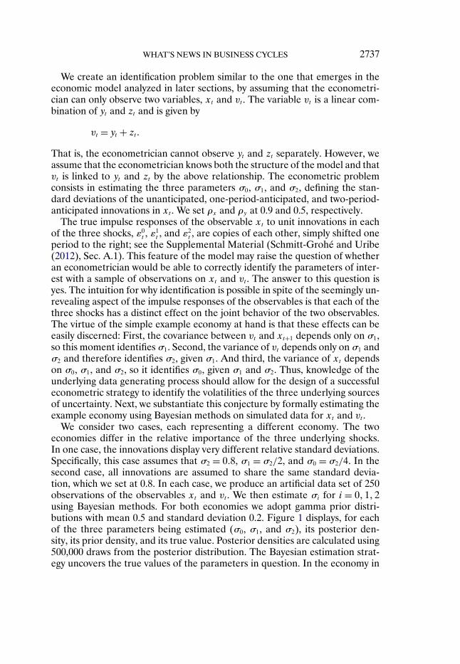
We create an identification problem similar to the one that emerges in theeconomic model analyzed in later sections, by assuming that the econometri-cian can only observe two variables, xt and vt . The variable vt is a linear com-bination of yt and zt and is given by
vt = yt + zt�That is, the econometrician cannot observe yt and zt separately. However, weassume that the econometrician knows both the structure of the model and thatvt is linked to yt and zt by the above relationship. The econometric problemconsists in estimating the three parameters σ0, σ1, and σ2, defining the stan-dard deviations of the unanticipated, one-period-anticipated, and two-period-anticipated innovations in xt . We set ρx and ρy at 0.9 and 0.5, respectively.
The true impulse responses of the observable xt to unit innovations in eachof the three shocks, ε0
t , ε1t , and ε2
t , are copies of each other, simply shifted oneperiod to the right; see the Supplemental Material (Schmitt-Grohé and Uribe(2012), Sec. A.1). This feature of the model may raise the question of whetheran econometrician would be able to correctly identify the parameters of inter-est with a sample of observations on xt and vt . The answer to this question isyes. The intuition for why identification is possible in spite of the seemingly un-revealing aspect of the impulse responses of the observables is that each of thethree shocks has a distinct effect on the joint behavior of the two observables.The virtue of the simple example economy at hand is that these effects can beeasily discerned: First, the covariance between vt and xt+1 depends only on σ1,so this moment identifies σ1. Second, the variance of vt depends only on σ1 andσ2 and therefore identifies σ2, given σ1. And third, the variance of xt dependson σ0, σ1, and σ2, so it identifies σ0, given σ1 and σ2. Thus, knowledge of theunderlying data generating process should allow for the design of a successfuleconometric strategy to identify the volatilities of the three underlying sourcesof uncertainty. Next, we substantiate this conjecture by formally estimating theexample economy using Bayesian methods on simulated data for xt and vt .
We consider two cases, each representing a different economy. The twoeconomies differ in the relative importance of the three underlying shocks.In one case, the innovations display very different relative standard deviations.Specifically, this case assumes that σ2 = 0�8, σ1 = σ2/2, and σ0 = σ2/4. In thesecond case, all innovations are assumed to share the same standard devia-tion, which we set at 0.8. In each case, we produce an artificial data set of 250observations of the observables xt and vt . We then estimate σi for i = 0�1�2using Bayesian methods. For both economies we adopt gamma prior distri-butions with mean 0.5 and standard deviation 0.2. Figure 1 displays, for eachof the three parameters being estimated (σ0, σ1, and σ2), its posterior den-sity, its prior density, and its true value. Posterior densities are calculated using500,000 draws from the posterior distribution. The Bayesian estimation strat-egy uncovers the true values of the parameters in question. In the economy in

2738 S. SCHMITT-GROHÉ AND M. URIBE
FIGURE 1.—Identification in the example economy. Posterior densities are shown with solidlines, prior densities with broken lines, and the true value of σi for i= 0�1�2 with vertical dottedlines. Posterior densities are calculated using 500,000 draws from the posterior distribution of therespective parameter. The left column of the figure corresponds to the case in which the trueparameter values are σ2 = 2σ1 = 4σ0 = 0�8. The right column corresponds to the case in whichthe true parameter values are σ2 = σ1 = σ0 = 0�8.
which (σ0�σ1�σ2) = (0�2�0�4�0�8), shown in the left column of Figure 1, theposterior means are, respectively, (0�24�0�40�0�79), with standard deviations(0�06�0�02�0�04). And in the economy in which (σ0�σ1�σ2) = (0�8�0�8�0�8),shown in the right column of Figure 1, the posterior means are, respectively,(0�75�0�73�0�77), with standard deviations (0�07�0�04�0�05). (The posteriormedians are very close to the corresponding posterior means.)
We apply two additional identification tests to this example model. One con-sists in examining the rank of the information matrix. We compute this matrixapplying the methodology proposed by Chernozhukov and Hong (2003). Wefind that, for both parameterizations of the data generating process, the in-formation matrix is full rank. The second test we apply is Iskrev’s (2010) testof identifiability. In essence, the Iskrev test checks whether the derivatives ofthe predicted autocovariogram of the observables with respect to the vector ofestimated parameters has rank equal to the length of the vector of estimatedparameters. For the example model developed in this section, the rank condi-tion can be shown analytically to hold globally. This result obtains even in the

WHAT’S NEWS IN BUSINESS CYCLES 2739
special cases in which either ρx or ρy or both are nil. See the SupplementalMaterial (Schmitt-Grohé and Uribe (2012), Sec. A.2) for a derivation of thisresult.
Although one cannot derive general conclusions from this example, it cer-tainly suggests that the identification of the standard deviations of the antic-ipated and unanticipated components of shocks is possible when there arefewer observables than shocks and even when the impulse responses of someof the observables to shocks hitting the economy at different anticipation hori-zons are shifted copies of one another.
3. THE MODEL
Consider an economy populated by a large number of identical, infinitelylived agents with preferences described by the lifetime utility function
E0
∞∑t=0
βtζtU(Vt)�(1)
where U denotes a period utility function, which we assume to belong to theCRRA family
U(V )= V 1−σ − 11 − σ �
with σ > 0. The variable ζt denotes an exogenous and stochastic preferenceshock in period t. This type of disturbance has been identified as an importantdriver of consumption fluctuations in most existing econometric estimationsof DSGE macroeconomic models (e.g., Smets and Wouters (2007), Justiniano,Primiceri, and Tambalotti (2008)). The argument of the period utility function,Vt , is assumed to be given by
Vt = Ct − bCt−1 −ψhθt St�(2)
where Ct denotes private consumption in period t, ht denotes hours workedin period t, and St is a geometric average of current and past habit-adjustedconsumption levels. The law of motion of St is postulated to be
St = (Ct − bCt−1)γS1−γ
t−1 �(3)
The parameter β ∈ (0�1) denotes the subjective discount factor, b ∈ [0�1) gov-erns the degree of internal habit formation, θ > 1 determines the Frisch elas-ticity of labor supply in the special case in which γ = b = 0, and ψ > 0 is ascale parameter. This preference specification is due to Jaimovich and Rebelo(2009). It introduces the parameter γ ∈ (0�1] governing the magnitude of thewealth elasticity of labor supply while preserving compatibility with long-run
2740 S. SCHMITT-GROHÉ AND M. URIBE
balanced growth. We modify the Jaimovich–Rebelo preference specificationto allow for internal habit formation in consumption. As γ→ 0, the argumentof the period utility function becomes linear in habit-adjusted consumptionand a function of hours worked, which, in the absence of habit formation, isthe preference specification considered by Greenwood, Hercowitz, and Huff-man (1988). This special case induces a supply of labor that depends only onthe current real wage, and, importantly, is independent of the marginal utilityof income. As a result, when γ and b are both small, anticipated changes inincome will not affect current labor supply. As γ increases, the wealth elastic-ity of labor supply rises. In the polar case in which γ is unity, Vt becomes aproduct of habit-adjusted consumption and a function of hours worked, whichis the preference specification most commonly studied in the closed-economybusiness-cycle literature. Because no econometric evidence exists on the valueof the parameter γ, an important byproduct of our investigation is to obtain anestimate of this parameter.
Households are assumed to own physical capital. The capital stock, de-noted Kt , is assumed to evolve over time according to the law of motion
Kt+1 = (1 − δ(ut)
)Kt + zIt It
[1 − S
(It
It−1
)]�(4)
where It denotes gross investment. Owners of physical capital can control theintensity with which the capital stock is utilized. Formally, we let ut measure ca-pacity utilization in period t. The effective amount of capital services suppliedto firms in period t is given by utKt . We assume that increasing the intensityof capital utilization entails a cost in the form of a faster rate of depreciation.Specifically, we assume that the depreciation rate, given by δ(ut), is an increas-ing and convex function of the rate of capacity utilization. We adopt a quadraticform for the function δ:
δ(u)= δ0 + δ1(u− 1)+ δ2
2(u− 1)2�
with δ0� δ1� δ2 > 0. The parameter δ2 defines the sensitivity of capacity utiliza-tion to variations in the rental rate of capital. The parameter δ1 governs thesteady-state level of ut . We set this parameter at a value consistent with a unitsteady-state value of ut . And the parameter δ0 corresponds to the rate of de-preciation of the capital stock in a deterministic steady state in which ut isunity.
The function S introduces investment adjustment costs of the form proposedby Christiano, Eichenbaum, and Evans (2005). We assume that the function Sevaluated at the steady-state growth rate of investment satisfies S = S′ = 0 andS′′ > 0. We focus on a quadratic specification of S:
S(x)= κ
2(x−μi)2
�

WHAT’S NEWS IN BUSINESS CYCLES 2741
where κ > 0 is a parameter and μi denotes the steady-state growth rate of in-vestment. The technology transforming investment goods into capital goods issubject to a transitory exogenous disturbance denoted by zIt . This type of shockhas recently been identified as an important source of aggregate fluctuationsby Justiniano, Primiceri, and Tambalotti (2011).
The sequential budget constraint of the household is given by
Ct +AtIt + Tt =W ∗t ht + rtutKt + Pt�(5)
The left-hand side of this expression represents the uses of income, given byconsumption, investment, and taxes. The variable At is an exogenous stochas-tic productivity shock shifting the (linear) technical rate of transformationof consumption goods into investment goods. In a decentralized competitiveequilibrium, At coincides with the relative price of new investment goods interms of consumption goods.4 We assume that the growth rate of At , denoted
μat ≡ At
At−1�
follows a stationary process and has a steady-state value of μa. The variableTt denotes lump-sum taxes. The right-hand side of the budget constraint rep-resents the sources of income, which consist of wage income, capital income,and lump-sum profits from the ownership of firms and membership in a laborunion. The variableW ∗
t denotes the wage rate received by households, the vari-able rt denotes the rental rate of an effective unit of capital, and the variablePt denotes profits.
The household’s optimization problem consists in choosing a set of stochas-tic processes {Ct� ht , St , Vt , It , Kt+1, ut}∞
t=0 to maximize (1) subject to (2)–(5),taking as given the stochastic processes {ζt , zIt , At , rt , W ∗
t , Tt , Pt}∞t=0, and the
initial conditions C−1, S−1, I−1, and K0.Motivated by earlier DSGE-based econometric studies of the U.S. business
cycle (e.g., Smets and Wouters (2007)), we introduce an exogenously time-varying markup in wages. This type of shock has been found to explain a largefraction of fluctuations in hours worked over the business cycle. To introduce atime-varying wage markup, we model the labor market as imperfectly competi-tive. On the demand side of this market, we assume that final-goods-producingfirms demand a composite labor input given by hct = [∫ 1
0 h1/(1+μt)jt dj]1+μt � where
hjt denotes the differentiated labor input of type j ∈ [0�1], and μt denotesthe markup in wages. We assume that μt is exogenous and stochastic, with
4The linear relationship between the relative price of investment and At and the implied ex-ogeneity of the relative price of investment could be broken by assuming that the technologyfor transforming consumption goods into investment goods is nonlinear. In Schmitt-Grohé andUribe (2011), we estimated the curvature of the technology for producing investment goods andfound that the data strongly favor a linear specification like the one maintained here.
2742 S. SCHMITT-GROHÉ AND M. URIBE
a steady-state value μ > 1. Let Wjt denote the wage posted by workers oftype j. The labor-cost minimization problem of a firm demanding hct unitsof the composite labor input is then given by min{hjt }
∫ 10 Wjthjt dj, subject to
[∫ 10 h
1/(1+μt)jt dj]1+μt ≥ hct � The solution of this cost minimization problem im-
plies a demand for labor of type j of the form hjt = hct (Wjt
Wt)−(1+μt)/μt � where
Wt = [∫ 10 W
−1/μtjt dj]−μt denotes the cost of one unit of the composite labor in-
put.The supply side of the labor market consists of monopolistically competitive
labor unions selling differentiated labor services to firms. The problem of theseller of labor of type j is to choose Wjt to maximize (Wjt − W ∗
t )hjt , subjectto the above labor demand schedule. Using that schedule to eliminate the la-bor input, hjt , from the objective function, the maximization problem of laborunion j takes the form maxWjt (Wjt −W ∗
t )hct (Wjt
Wt)−(1+μt)/μt � The optimality condi-
tion associated with this problem is W ∗t = Wjt
1+μt � It follows from this expressionthat the wage rate the union pays to its members is smaller than the wage ratefirms pay to the unions. Also apparent from this expression is that all laborunions charge the same wage rate Wt . In turn, the fact that all types of laborcommand the same wage implies, by the demand functions for specialized la-bor services, that firms will demand identical quantities of each type of labor,hjt = hct for all j. Profits of union j, given by μt/(1 + μt)Wjthjt , are assumedto be rebated to households in a lump-sum fashion. Finally, in equilibrium, wehave that the total number of hours allocated by the unions must equal total la-bor supply, or
∫ 10 hjt dj = ht , which, since hjt = hct for all j, implies that hct = ht�
This completes the description of the labor market.Output, denoted Yt , is produced with a homogeneous-of-degree-1 produc-
tion function that takes as inputs capital, labor services, and a fixed factor thatcan be interpreted as land or organizational capital. The fixed factor of produc-tion introduces decreasing returns to scale in the variable factors of production.Jaimovich and Rebelo (2009) suggested that a small amount of decreasing re-turns to scale allows for a positive response of the value of the firm to futureexpected increases in productivity. The production technology is buffeted bya transitory productivity shock, denoted zt , and by a permanent productivityshock, denoted Xt . Formally, the production function is given by
Yt = ztF(utKt�Xtht�XtL)�(6)
where F is taken to be of the Cobb–Douglas form: F(a�b� c)= aαkbαhc1−αk−αh�where αk�αh ∈ (0�1) are parameters satisfying αk +αh ≤ 1. The growth rate ofthe permanent productivity shock, denoted
μxt ≡ Xt
Xt−1�

WHAT’S NEWS IN BUSINESS CYCLES 2743
is assumed to be an exogenous, stationary stochastic process with a steady-statevalue equal to μx.
The government is assumed to consume an exogenous and stochasticamount of goods Gt each period and to finance these expenditures by levy-ing lump-sum taxes. We assume that government spending, Gt , displays astochastic trend given by XG
t . We let gt ≡ Gt/XGt denote detrended govern-
ment spending. The trend in government spending is assumed to be cointe-grated with the trend in output, denoted XY
t . This assumption ensures thatthe share of government spending in output is stationary. However, we allowfor the possibility that the trend in government spending is smoother than thetrend in output. Specifically, we assume that XG
t = (XGt−1)
ρxg(XYt−1)
1−ρxg � whereρxg ∈ [0�1) is a parameter governing the smoothness of the trend in govern-ment spending. In the present model, the trend in output can be shown to begiven by XY
t =XtAαk/(αk−1)t . Notice that XG
t resides in the information set ofperiod t − 1. This fact, together with the assumption that gt is autoregressive,implies the absence of contemporaneous feedback from any endogenous orexogenous variable to the level of government spending. At the same time, themaintained specification of the government spending process allows for laggedfeedback from changes in the trend path of output.
A competitive equilibrium is a set of stochastic processes {Ct , ht , It ,Kt+1, Yt ,ut , Qt , Λt , St , Vt , Πt}∞
t=0 satisfying
Kt+1 = (1 − δ(ut)
)Kt + zIt It
[1 − S
(It
It−1
)]�
Ct +AtIt +Gt = Yt�Yt = ztF(utKt�Xtht�XtL)�
Vt = (Ct − bCt−1)−ψhθt St�St = (Ct − bCt−1)
γS1−γt−1 �[
ζtU′(Vt)−Πtγ
St
Ct − bCt−1
]
−βbEt[ζt+1U
′(Vt+1)−Πt+1γSt+1
Ct+1 − bCt]
=Λt�
θψζtU′(Vt)hθ−1
t St =Λt
ztXtF2(utKt�Xtht�XtL)
1 +μt �
Πt =ψζtU ′(Vt)hθt +β(1 − γ)EtΠt+1St+1
St�
QtΛt = βEtΛt+1
[zt+1ut+1F1(ut+1Kt+1�Xt+1ht+1�Xt+1L)
+Qt+1
(1 − δ(ut+1)
)]�

2744 S. SCHMITT-GROHÉ AND M. URIBE
ztF1(utKt�Xtht�XtL)=Qtδ′(ut)�
AtΛt =QtΛtzIt
[1 − S
(It
It−1
)− It
It−1S′
(It
It−1
)]
+βEtQt+1Λt+1zIt+1
(It+1
It
)2
S′(It+1
It
)�
given the set of exogenous stochastic processes {zt , Xt , Gt , At , zIt , ζt , μt}∞t=0,
and the initial conditions K0, I−1, C−1, and S−1. The variables Λt , Πt , and QtΛt
represent, respectively, the Lagrange multiplier associated with the sequentialbudget constraint, the evolution of St , and the evolution of physical capital inthe household’s optimization problem.
The variableQt can be interpreted as the relative price of installed capital inperiod t available for production in period t+1 in terms of consumption goodsof period t. This relative price is also known as marginal Tobin’s Q. A relatedconcept is the value of the firm. Let V F
t denote the value of the firm at thebeginning of period t. Then one can write V F
t recursively as V Ft = Yt −Wtht −
AtIt +βEt Λt+1ΛtV Ft+1� This expression states that the value of the firm equals the
present discounted value of current and future expected dividends.
4. INTRODUCING ANTICIPATED SHOCKS
Our model of the business cycle is driven by seven exogenous forces: thestationary neutral productivity shock zt , the nonstationary neutral productivityshock Xt , the stationary investment-specific productivity shock zIt , the nonsta-tionary investment-specific productivity shock At , the government spendingshock Gt , the wage-markup shock μt , and the preference shock ζt . We assumethat all of these forces are subject to anticipated as well as unanticipated in-novations. We study a formulation with four- and eight-quarter anticipatedshocks. This choice is motivated by two considerations. First, we would like tocapture a relatively long anticipation horizon (in this case, two years). Second,we wish to avoid the proliferation of estimated parameters. Each anticipationhorizon adds one parameter per driving force, namely, the standard deviationof the innovation at that particular anticipation horizon. Under the currentspecification, we are estimating 21 standard deviations. This is 14 parametersmore than in a specification without anticipation. It would be of interest tostudy the robustness of our results regarding the importance of anticipation tomaking the anticipation structure longer and denser.
We assume that all exogenous shocks xt , for x= z�μx�μa�g� zI� ζ�μ, evolveover time according to the following law of motion:
ln(xt/x)= ρx ln(xt−1/x)+ εx�t�εx�t = ε0
x�t + ε4x�t−4 + ε8
x�t−8�

WHAT’S NEWS IN BUSINESS CYCLES 2745
where εjx�t for j = 0�4, and 8 is assumed to be an i.i.d. normal disturbance withmean zero and standard deviation σjx.
The innovation εjx�t denotes j-period anticipated changes in the logarithmof xt . For example, ε4
x�t−4 is an innovation to the level of xt that materializesin period t, but that agents learn about in period t − 4. Therefore, ε4
x�t−4 isin the period t − 4 information set of economic agents but results in an actualchange in the variable xt only in period t. We thus say that ε4
x�t−4 is a four-periodanticipated innovation in xt . The disturbance εjx�t has mean zero, standard de-viation σjx, and is uncorrelated across time and across anticipation horizons.That is, Eεjx�tεkx�t−m = 0 for k� j = 0�4�8 and m > 0, and Eεjx�tεkx�t = 0 for anyk �= j. These assumptions imply that the error term εx�t is unconditionally meanzero and serially uncorrelated, that is, Eεx�t = 0 and Eεx�tεx�t−m = 0, form> 0.Moreover, the error term εx�t is unforecastable given only past realizations ofitself. That is, E(εx�t+m|εx�t� εx�t−1� � � �)= 0, for m> 0. Note that the proposedprocess for εx�t does not contain any moving average component.
The key departure of this paper from standard business-cycle analysis is theassumption that economic agents have an information set larger than one sim-ply containing current and past realizations of εx�t . In particular, agents areassumed to observe, in period t, current and past values of the innovations ε0
x�t ,ε4x�t , and ε8
x�t . That is, agents can forecast future values of εx�t as follows:
Etεx�t+k =⎧⎨⎩ε4x�t+k−4 + ε8
x�t+k−8� if 1 ≤ k≤ 4,ε8x�t+k−8� if 4<k≤ 8,
0� if k > 8.
Because agents are forward looking, they use the information contained in therealizations of the various innovations εjx�t in their current choices of consump-tion, investment, hours worked, and asset holdings. It is precisely this forward-looking behavior of economic agents that allows an econometrician to identifythe volatilities of the anticipated innovations εjx�t , even though the econometri-cian himself cannot directly observe these innovations.
4.1. Autoregressive Representation of Anticipated Shocks
The law of motion of the exogenous process xt can be written recursively asa first-order linear stochastic difference equation of the form
x̃t+1 =Mx̃t +ηνx�t+1�
where νx�t = [ν0x�t ν
4x�t ν
8x�t
]′distributes normal i.i.d. with mean zero and
variance–covariance matrix equal to the identity matrix. The vector x̃t andthe matrices M and η are given in the Supplemental Material (Schmitt-Grohéand Uribe (2012), Sec. A.4).

2746 S. SCHMITT-GROHÉ AND M. URIBE
The central goal of our investigation is to econometrically estimate thenonzero elements of η, which are given by the standard deviations of the antic-ipated and unanticipated components of each of the seven exogenous shocks,σ0j , σ4
j and σ8j , for j = z�μx�μa� zI� g� ζ�μ.
4.2. Accommodating Revisions
We view the structure given above to anticipated and unanticipated inno-vations as just one of potentially many ways to model information diffusion.Our approach is flexible enough to accommodate revisions in announcements.These revisions capture situations such as announced productivity improve-ments that do not pan out or wage negotiations that start out as promisingfor workers (i.e., the announcement of a future increase in wage markups)but then go sour. Consider, for example, a positive realization of the innova-tion ε8
z�t . This shock represents the announcement in period t of an improve-ment in productivity that will take place in period t+8. Under our formulation,this announcement is subject to two revisions. The first revision takes place inperiod t + 4. Suppose, for instance, that the realization of ε4
z�t+4 is negative.This is equivalent to the announcement that the productivity improvement an-nounced in period t will not materialize as expected. At this point, the economymay enter into a recession even though none of the economic fundamentals haschanged. The second revision of the announcement of period t occurs in pe-riod t+8. Suppose that the realization of ε0
z�t+8 is negative and offsets the priortwo announcements ε8
z�t + ε4z�t+4. This is a situation in which agents learn that
the earlier optimistic outlook for productivity did not pan out at all. The econ-omy may experience, at this point, a double dip recession. Like the one thattook place in period t + 4, the t + 8 recession occurs without any changes inobserved economic fundamentals. This interpretation suggests an equivalentbut more parsimonious representation of anticipation in which state variablescollect all prior innovations that will materialize in a given horizon. One ad-vantage of this formulation is that it reduces the number of exogenous statevariables in the system. We present this formulation, which was suggested to usby an anonymous referee, in the Supplemental Material (Schmitt-Grohé andUribe (2012), Sec. A.4).
4.3. Inducing Stationarity and Solution Method
The exogenous forcing processes Xt and At display stochastic trends. Theserandom trends are inherited by the endogenous variables of the model. We fo-cus our attention on equilibrium fluctuations around these stochastic trends.To this end, we perform a stationarity-inducing transformation of the endoge-nous variables by dividing them by their trend component.
We compute a log-linear approximation to the equilibrium dynamics of themodel. We have already shown how to express the law of motion of the ex-ogenous driving forces of the model in a first-order autoregressive form. Then,

WHAT’S NEWS IN BUSINESS CYCLES 2747
using familiar perturbation techniques (e.g., Schmitt-Grohé and Uribe (2004)),one can write the equilibrium dynamics of the model up to first order as
xt+1 = hxxt +ηνt+1�(7)
yt = gxxt + ξmt�(8)
where xt is a vector of endogenous and exogenous state variables, yt is the vec-tor of observables, νt is a vector of structural disturbances distributed N(0� I),andmt is a vector of measurement errors distributedN(0� I). The matrices hx,gx, η, and ξ are functions of the structural parameters of the model.
5. ESTIMATING ANTICIPATED SHOCKS
We use Bayesian and classical maximum likelihood (ML) methods to esti-mate a subset of the deep structural parameters of the model. Of particularimportance among the estimated parameters are those defining the stochasticprocesses of anticipated and unanticipated innovations. The parameters thatare not estimated are calibrated in a standard fashion.
5.1. Calibrated Parameters
Table I presents the values assigned to the calibrated parameters. The timeunit is defined to be one quarter. We assign a value of 1 to σ , the parameterdefining the curvature of the period utility function. This value is standard inthe business-cycle literature. Following Jaimovich and Rebelo (2009), we as-sume a degree of decreasing returns to scale of 10 percent. We set the capitalelasticity of the production function, αk, to 0.225. This value, together with the
TABLE I
CALIBRATED PARAMETERSa
Parameter Value Description
β 0�99 Subjective discount factorσ 1 Intertemporal elasticity of substitutionαk 0�225 Capital shareαh 0�675 Labor shareδ0 0�025 Steady-state depreciation rateu 1 Steady-state capacity utilization rateμy 1�0045 Steady-state gross per capita GDP growth rateμa 0�9957 Steady-state gross growth rate of price of investmentG/Y 0�2 Steady-state share of government consumption in GDPh 0�2 Steady-state hoursμ 0�15 Steady-state wage markup
aThe time unit is one quarter.

2748 S. SCHMITT-GROHÉ AND M. URIBE
assumed degree of decreasing returns to scale, implies that the labor share is0.67, which is in line with existing business-cycle studies. We assume a depreci-ation rate of 2.5 percent per quarter. We calibrate the parameter δ1 to ensurethat capacity utilization, u, equals unity in the steady state. We set the discountfactor β at 0.99, a value commonly used in related studies. We calibrate thesteady-state growth rates of per capita output and of the relative price of in-vestment, μy and μa, respectively, to be 0.45 and −0�43 percent per quarter.These two figures correspond to the average growth rates of per capita out-put and the price of investment over the period 1955:Q2 to 2006:Q4. Follow-ing Justiniano, Primiceri, and Tambalotti (2008), we set the steady-state wagemarkup, μ, at 15 percent. We set the parameter ψ of the utility function at avalue consistent with a steady-state fraction of time dedicated to remuneratedlabor of 20 percent. Finally, we set the share of government purchases in out-put equal to 20 percent, which is in line with the average government spendingshare in our sample.
5.2. Bayesian and Classical Maximum Likelihood Estimation
We perform classical maximum likelihood and Bayesian estimations of thenoncalibrated structural parameters of the model. Specifically, given the sys-tem of linear stochastic difference equations (7) and (8) describing the equi-librium dynamics of the model up to first order, it is straightforward to numer-ically evaluate the likelihood function of the data given the vector of estimatedparameters, which we denote by L(Y |Θ), where Y is the data sample and Θis the vector of parameters to be estimated. This object is the basis of ourmaximum likelihood estimation of the parameter vector Θ. Given a prior pa-rameter distribution P(Θ), the posterior likelihood function of the parameterΘ given the data, which we denote by L(Θ|Y), is proportional to the productL(Y |Θ)P(Θ). This object forms the basis of our Bayesian estimation. In par-ticular, following the methodology described in An and Schorfheide (2007),we use the Metropolis–Hastings algorithm to obtain draws from the posteriordistribution of Θ.
The vector of estimated parameters, Θ, contains the parameters definingthe stochastic process for anticipated and unanticipated innovations, namely,ρj and σij for i = 0�4�8 and j = z�μx� zI�μa�g�μ�ζ. In addition, the parame-ter vector Θ includes the parameter ρxg governing the smoothness in the trendcomponent of government spending, the parameter γ related to the wealthelasticity of labor supply, the preference parameter b defining habits in con-sumption, the preference parameter θ related to the Frisch elasticity of laborsupply, the parameter δ2 governing the convexity of the cost of adjusting ca-pacity utilization, and the parameter κ governing the cost of adjusting invest-ment.
We estimate the model on U.S. quarterly data ranging from 1955:Q2 to2006:Q4. The data include seven time series: the growth rates of per capita real
WHAT’S NEWS IN BUSINESS CYCLES 2749
GDP, real consumption, real investment, real government expenditure, andhours, and the growth rates of total factor productivity and the relative priceof investment. Our set of observables differs from those employed in existinglikelihood-based estimates of DSGE macroeconomic models in that it includesboth a time series for total factor productivity and a time series for the relativeprice of investment. Naturally, the inclusion of these two time series restrictsthe freedom of neutral and investment-specific productivity shocks to explainthe behavior of observables other than total factor productivity and the rela-tive price of investment themselves. This is because the estimation procedurehas a tendency to pick stochastic processes for neutral and investment-specificproductivity shocks geared toward accounting for movements in their respec-tive observable counterparts, namely, total factor productivity and the price ofinvestment.
We assume that output growth is measured with error. Allowing for mea-surement error in output is required by the fact that, up to first order, the re-source constraint of the model economy postulates a linear restriction amongthe seven observables. Formally, the vector of observable variables is givenby
vector of observables =
⎡⎢⎢⎢⎢⎢⎢⎢⎣
� ln(Yt)� ln(Ct)� ln(AtIt)� ln(ht)� ln(Gt)� ln(TFPt)� ln(At)
⎤⎥⎥⎥⎥⎥⎥⎥⎦
× 100 +
⎡⎢⎢⎢⎢⎢⎢⎢⎣
εmey�t
000000
⎤⎥⎥⎥⎥⎥⎥⎥⎦�
where � denotes the temporal difference operator, and TFPt ≡ ztX1−αkt de-
notes total factor productivity. The measurement error in output growth,εmey�t , is assumed to be an i.i.d. innovation with mean zero and standard de-
viation σmegy . The Appendix provides more detailed information about the
data used in the estimation of the model. The vector of estimated param-eters Θ also includes the standard deviation of the measurement error,σmegy .Table II displays the assumed prior distribution P(Θ) of the estimated struc-
tural parameters contained in the vector Θ. We assume gamma distributionsfor the standard deviations of all 21 innovations of the model. The reasonwe use gamma distributions instead of inverse-gamma distributions, which aremore commonly used as priors for standard deviations, is to allow for a pos-itive density at zero for the standard deviations of anticipated shocks. In thisway, our priors allow for the possibility that individual anticipated shocks notmatter at all. For each of the seven shocks in the model, the prior distributionsof the standard deviations of the two anticipated components are assumed tobe identical. We assume that, for each of the seven shocks, the variance of
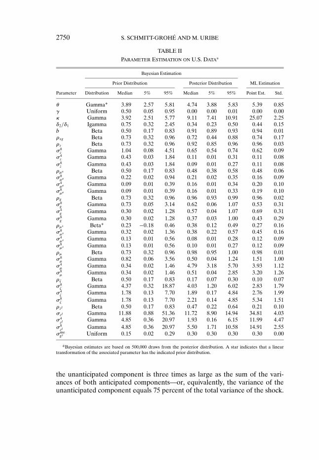
2750 S. SCHMITT-GROHÉ AND M. URIBE
TABLE II
PARAMETER ESTIMATION ON U.S. DATAa
Bayesian Estimation
Prior Distribution Posterior Distribution ML Estimation
Parameter Distribution Median 5% 95% Median 5% 95% Point Est. Std.
θ Gamma* 3�89 2�57 5�81 4�74 3�88 5�83 5�39 0�85γ Uniform 0�50 0�05 0�95 0�00 0�00 0�01 0�00 0�00κ Gamma 3�92 2�51 5�77 9�11 7�41 10�91 25�07 2�25δ2/δ1 Igamma 0�75 0�32 2�45 0�34 0�23 0�50 0�44 0�15b Beta 0�50 0�17 0�83 0�91 0�89 0�93 0�94 0�01ρxg Beta 0�73 0�32 0�96 0�72 0�44 0�88 0�74 0�17ρz Beta 0�73 0�32 0�96 0�92 0�85 0�96 0�96 0�03σ0z Gamma 1�04 0�08 4�51 0�65 0�54 0�74 0�62 0�09σ4z Gamma 0�43 0�03 1�84 0�11 0�01 0�31 0�11 0�08σ8z Gamma 0�43 0�03 1�84 0�09 0�01 0�27 0�11 0�08ρμa Beta 0�50 0�17 0�83 0�48 0�38 0�58 0�48 0�06σ0μa Gamma 0�22 0�02 0�94 0�21 0�02 0�35 0�16 0�09σ4μa Gamma 0�09 0�01 0�39 0�16 0�01 0�34 0�20 0�10σ8μa Gamma 0�09 0�01 0�39 0�16 0�01 0�33 0�19 0�10ρg Beta 0�73 0�32 0�96 0�96 0�93 0�99 0�96 0�02σ0g Gamma 0�73 0�05 3�14 0�62 0�06 1�07 0�53 0�31σ4g Gamma 0�30 0�02 1�28 0�57 0�04 1�07 0�69 0�31σ8g Gamma 0�30 0�02 1�28 0�37 0�03 1�00 0�43 0�29ρμx Beta* 0�23 −0�18 0�46 0�38 0�12 0�49 0�27 0�16σ0μx Gamma 0�32 0�02 1�36 0�38 0�22 0�57 0�45 0�16σ4μx Gamma 0�13 0�01 0�56 0�08 0�01 0�28 0�12 0�09σ8μx Gamma 0�13 0�01 0�56 0�10 0�01 0�27 0�12 0�09ρμ Beta 0�73 0�32 0�96 0�98 0�95 1�00 0�98 0�01σ0μ Gamma 0�82 0�06 3�56 0�50 0�04 1�24 1�51 1�00σ4μ Gamma 0�34 0�02 1�46 4�79 3�18 5�70 3�93 1�12σ8μ Gamma 0�34 0�02 1�46 0�51 0�04 2�85 3�20 1�26ρζ Beta 0�50 0�17 0�83 0�17 0�07 0�30 0�10 0�07σ0ζ Gamma 4�37 0�32 18�87 4�03 1�20 6�02 2�83 1�79σ4ζ Gamma 1�78 0�13 7�70 1�89 0�17 4�84 2�76 1�99σ8ζ Gamma 1�78 0�13 7�70 2�21 0�14 4�85 5�34 1�51ρzI Beta 0�50 0�17 0�83 0�47 0�22 0�64 0�21 0�10σzI Gamma 11�88 0�88 51�36 11�72 8�90 14�94 34�81 4�03σ4zI
Gamma 4�85 0�36 20�97 1�93 0�16 6�15 11�99 4�47σ8zI
Gamma 4�85 0�36 20�97 5�50 1�71 10�58 14�91 2�55σmegy Uniform 0�15 0�02 0�29 0�30 0�30 0�30 0�30 0�00
aBayesian estimates are based on 500,000 draws from the posterior distribution. A star indicates that a lineartransformation of the associated parameter has the indicated prior distribution.
the unanticipated component is three times as large as the sum of the vari-ances of both anticipated components—or, equivalently, the variance of theunanticipated component equals 75 percent of the total variance of the shock.

WHAT’S NEWS IN BUSINESS CYCLES 2751
Formally, at the mean of the prior distributions, we have that
(σ0x)
2
(σ0x)
2 + (σ4x)
2 + (σ8x)
2= 0�75; x= z�μx� zI�μa�g�μ�ζ�
We set the total prior variance of the seven shocks so that the model predic-tions for standard deviations, serial correlations, and correlations with outputgrowth of the seven observables are broadly in line with the data when theremaining structural parameters are set at their maximum likelihood point es-timates. We complete the specification of the prior distributions of the stan-dard deviations of the 21 innovations by imposing a common unit coefficientof variation on all of these distributions. This choice of priors gives rise to priorprobability densities for the share of anticipated shocks in the variance of keymacroeconomic variables that are quite dispersed (see Figure 2 and Table Vbelow).
The prior distributions for the remaining estimated structural parameters ofthe model follow broadly those used in the related literature. An exceptionis the preference parameter γ, controlling the income elasticity of labor sup-ply, which, to our knowledge, has not been previously estimated. We adopt auniform prior distribution for γ, with a support spanning the interval (0�1].Our maximum likelihood and Bayesian estimates of γ are consistent with eachother and both point to a value close to zero. This estimate implies that, in theabsence of habit formation, the model would display a labor supply schedulewith a near-zero wealth elasticity, providing support for the preference spec-ification proposed by Greenwood, Hercowitz, and Huffman (1988). Finally,we choose a uniform prior distribution for the standard deviation of measure-ment error in output growth. We restrict the measurement error to account forat most 10 percent of the variance of output growth.
5.3. Model Fit
Table III presents the model’s predictions regarding standard deviations,correlations with output growth, and serial correlations of the seven time seriesincluded as observables in the estimation. Predicted second moments are com-puted unconditionally. When the model is estimated using maximum likeli-hood, the population second moments are computed using the point estimatesof the structural parameters. When the model is estimated using Bayesianmethods, the table reports the median of the posterior distribution of the pop-ulation second moments. For comparison, the table also shows the correspond-ing empirical second moments calculated over the sample 1955:Q2 to 2006:Q4.
The second moments predicted by the estimated model are quite similarunder maximum likelihood and Bayesian estimation. Overall, the estimatedmodel matches well the empirical second moments. In particular, it replicatesthe observed levels of volatility in consumption, investment, hours, government

2752 S. SCHMITT-GROHÉ AND M. URIBE
TABLE III
MODEL PREDICTIONSa
Statistic Y C I h G TFP A
Standard DeviationsData 0.91 0.51 2.28 0.84 1.14 0�75 0�41Model—Bayesian estimation 0.73 0.58 2.69 0.85 1.13 0�79 0�40Model—ML estimation 0.67 0.53 2.28 0.79 1.01 0�76 0�36
Correlations With Output GrowthData 1.00 0.50 0.69 0.72 0.25 0�40 −0�12Model—Bayesian estimation 1.00 0.58 0.69 0.42 0.33 0�28 0�01Model—ML estimation 1.00 0.60 0.67 0.38 0.34 0�22 0�04
AutocorrelationsData 0.28 0.20 0.53 0.60 0.05 −0�01 0�49Model—Bayesian estimation 0.43 0.39 0.60 0.14 0.02 0�03 0�47Model—ML estimation 0.36 0.34 0.52 0.09 0.03 0�05 0�48
aBayesian estimates are medians of 500,000 draws from the posterior distributions of the corresponding populationsecond moments. The columns labeled Y , C , I, h, G, TFP, and A refer, respectively, to the growth rates of output,private consumption, investment, hours, government consumption, total factor productivity, and the relative price ofinvestment.
spending, total factor productivity, and the relative price of investment, andslightly underpredicts the volatility of output. The model also captures wellthe autocorrelations and contemporaneous correlations with output growthof consumption, investment, government spending, total factor productivity,and the relative price of investment. The most notable discrepancies betweenmodel predictions and data can be found in the serial correlation of the growthrate of hours and, to a lesser extent, in the correlation of hours and output.
5.4. Identifiability and Identification
To gauge the ability of our empirical strategy to identify the parameter vec-tor Θ, we perform three identification tests. First, we check for the identi-fiability of the estimated parameter vector Θ by applying the test proposedby Iskrev (2010). See the Supplemental Material (Schmitt-Grohé and Uribe(2012), Sec. A.3) for details on the implementation of this test. We find thatthe derivative of the vectorized predicted autocovariogram of the vector ofobservables with respect to Θ has full column rank when evaluated at the max-imum likelihood estimate or at the posterior mean or median of the Bayesianestimate. Full column rank obtains starting with the inclusion of covariancesof order 0 and 1. According to this test, therefore, the parameter vector Θ isidentifiable in the neighborhood of our estimate. Specifically, the test resultindicates that, in the neighborhood of our estimate of Θ, all values of Θ dif-ferent from our estimate give rise to autocovariograms that are different fromthe one associated with our estimate of Θ.

WHAT’S NEWS IN BUSINESS CYCLES 2753
Our second identification test consists in examining the rank of the informa-tion matrix. We compute this matrix following the methodology proposed byChernozhukov and Hong (2003). We find that the information matrix is fullrank, which suggests that, given our data sample, the parameter vector Θ isindeed identified.
Our third identification test consists in applying our estimation strategy toartificial data stemming from the DSGE model to show that our proposed em-pirical approach can recover the underlying parameters. Specifically, we cal-ibrate our baseline DSGE model using the posterior mean of the estimatedparameters. Then we generate artificial data for the seven observables. The ar-tificial data set contains 207 observations, which is the length of the actual dataset used in our study. We add measurement error to the time series of outputgrowth of the size implied by our calibration. Then we estimate the model us-ing ML and Bayesian methods, following exactly the same procedures and codeas we do in our estimation using real data. The Bayesian estimates are basedon the same prior distributions as those used in our estimation of the modelon actual data. At no point does the estimation procedure make use of ourknowledge of the true parameter values. Table IV displays the results of thisidentification test. The table reports the true value of the parameter vector,the maximum likelihood estimate, and the posterior median, 5th percentile,and 95th percentile computed from 500,000 draws from the posterior distribu-tion. In our view, given the size of the artificial data sample, both the ML andBayesian estimation procedures capture the true parameter values reasonablywell.
6. THE IMPORTANCE OF ANTICIPATED SHOCKS
In this section, we present model-based evidence on the importance of an-ticipated shocks as sources of business-cycle fluctuations through a number ofperspectives.
6.1. Bayesian Estimate
Table V displays the share of the unconditional variances of output growth,consumption growth, investment growth, and hours growth that, according toour Bayesian estimation, can be accounted for by anticipated shocks. Panel 2of the table displays the median posterior share as well as the 5th and 95thpercentiles computed from 500,000 draws from the posterior distribution ofthe vector of estimated structural parameters. The table shows that antici-pated shocks account for 41 percent of the variance of output growth and for77 percent of movements in hours. This finding is of interest in light of thefact that the long existing literature on business cycles has implicitly attributedone hundred percent of the variance of output and hours growth to unantici-pated shocks. Our results represent an example of a model economy in which,

2754 S. SCHMITT-GROHÉ AND M. URIBE
TABLE IV
ESTIMATION ON ARTIFICIAL DATAa
Bayesian Estimation
TrueValue
MLPoint
Estimate
Prior Distribution Posterior Distribution
Parameter Distribution Median 5% 95% Median 5% 95%
θ 4�78 6�25 Gamma* 3�89 2�57 5�81 4.82 3.92 4.90γ 0�00 0�00 Uniform 0�50 0�05 0�95 0.00 0.00 0.01κ 9�12 9�49 Gamma 3�92 2�51 5�77 5.44 4.09 6.97δ2/δ1 0�35 0�67 Igamma 0�75 0�32 2�45 0.39 0.25 0.58b 0�91 0�96 Beta 0�50 0�17 0�83 0.91 0.88 0.93ρxg 0�70 0�76 Beta 0�73 0�32 0�96 0.65 0.37 0.82ρz 0�91 0�91 Beta 0�73 0�32 0�96 0.87 0.78 0.93σ0z 0�65 0�49 Gamma 1�04 0�08 4�51 0.63 0.40 0.76σ4z 0�13 0�20 Gamma 0�43 0�03 1�84 0.17 0.01 0.45σ8z 0�11 0�32 Gamma 0�43 0�03 1�84 0.21 0.02 0.48ρμa 0�48 0�43 Beta 0�50 0�17 0�83 0.44 0.33 0.55σ0μa 0�20 0�17 Gamma 0�22 0�02 0�94 0.26 0.06 0.33σ4μa 0�16 0�17 Gamma 0�09 0�01 0�39 0.10 0.01 0.28σ8μa 0�16 0�21 Gamma 0�09 0�01 0�39 0.09 0.01 0.26ρg 0�96 0�94 Beta 0�73 0�32 0�96 0.92 0.85 0.97σ0g 0�59 0�00 Gamma 0�73 0�05 3�14 0.53 0.04 0.90σ4g 0�56 0�31 Gamma 0�30 0�02 1�28 0.35 0.02 0.86σ8g 0�43 0�86 Gamma 0�30 0�02 1�28 0.41 0.03 0.89ρμx 0�35 0�20 Beta* 0�23 −0�18 0�46 0.28 0.02 0.97σ0μx 0�39 0�68 Gamma 0�32 0�02 1�36 0.43 0.19 0.65σ4μx 0�10 0�00 Gamma 0�13 0�01 0�56 0.11 0.01 0.37σ8μx 0�11 0�04 Gamma 0�13 0�01 0�56 0.11 0.01 0.35ρμ 0�97 0�97 Beta 0�73 0�32 0�96 0.95 0.91 0.99σ0μ 0�55 0�00 Gamma 0�82 0�06 3�56 1.15 0.08 2.88σ4μ 4�65 5�00 Gamma 0�34 0�02 1�46 3.72 0.60 4.69σ8μ 0�81 1�97 Gamma 0�34 0�02 1�46 0.41 0.02 3.95ρζ 0�18 0�13 Beta 0�50 0�17 0�83 0.17 0.07 0.29σ0ζ 3�85 6�11 Gamma 4�37 0�32 18�87 3.58 0.35 5.59σ4ζ 2�15 4�88 Gamma 1�78 0�13 7�70 1.51 0.10 4.19σ8ζ 2�28 5�71 Gamma 1�78 0�13 7�70 2.09 0.16 5.27ρzI 0�45 0�17 Beta 0�50 0�17 0�83 0.52 0.19 0.75σ0zI
11�73 13�16 Gamma 11�88 0�88 51�36 6.89 4.71 9.62σ4zI
2�45 8�48 Gamma 4�85 0�36 20�97 2.35 0.16 8.35σ8zI
5�69 9�05 Gamma 4�85 0�36 20�97 2.20 0.19 6.96σmegy 0�30 0�28 Uniform 0�15 0�02 0�29 0.28 0.26 0.30
aThe true parameter value is the posterior mean of the Bayesian estimation on actual data. The posterior median,5th percentile, and 95th percentile estimated on artificial data were computed over 500,000 draws from the posteriordistribution of the estimated parameter vector.
when one allows for unanticipated and anticipated disturbances to play sepa-rate roles, the latter emerge as an important driving force.
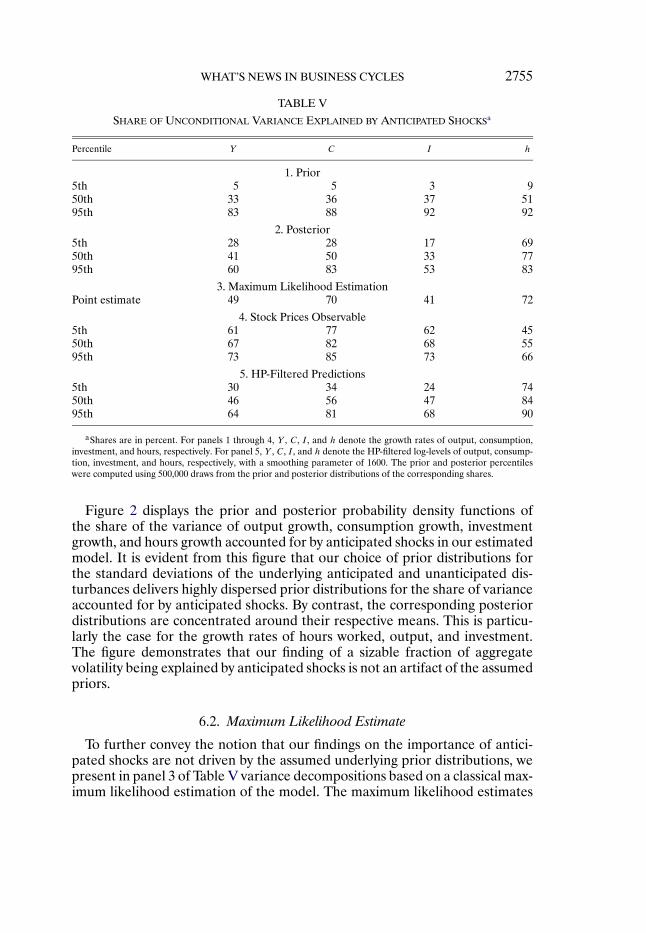
WHAT’S NEWS IN BUSINESS CYCLES 2755
TABLE V
SHARE OF UNCONDITIONAL VARIANCE EXPLAINED BY ANTICIPATED SHOCKSa
Percentile Y C I h
1. Prior5th 5 5 3 950th 33 36 37 5195th 83 88 92 92
2. Posterior5th 28 28 17 6950th 41 50 33 7795th 60 83 53 83
3. Maximum Likelihood EstimationPoint estimate 49 70 41 72
4. Stock Prices Observable5th 61 77 62 4550th 67 82 68 5595th 73 85 73 66
5. HP-Filtered Predictions5th 30 34 24 7450th 46 56 47 8495th 64 81 68 90
aShares are in percent. For panels 1 through 4, Y , C , I, and h denote the growth rates of output, consumption,investment, and hours, respectively. For panel 5, Y , C , I, and h denote the HP-filtered log-levels of output, consump-tion, investment, and hours, respectively, with a smoothing parameter of 1600. The prior and posterior percentileswere computed using 500,000 draws from the prior and posterior distributions of the corresponding shares.
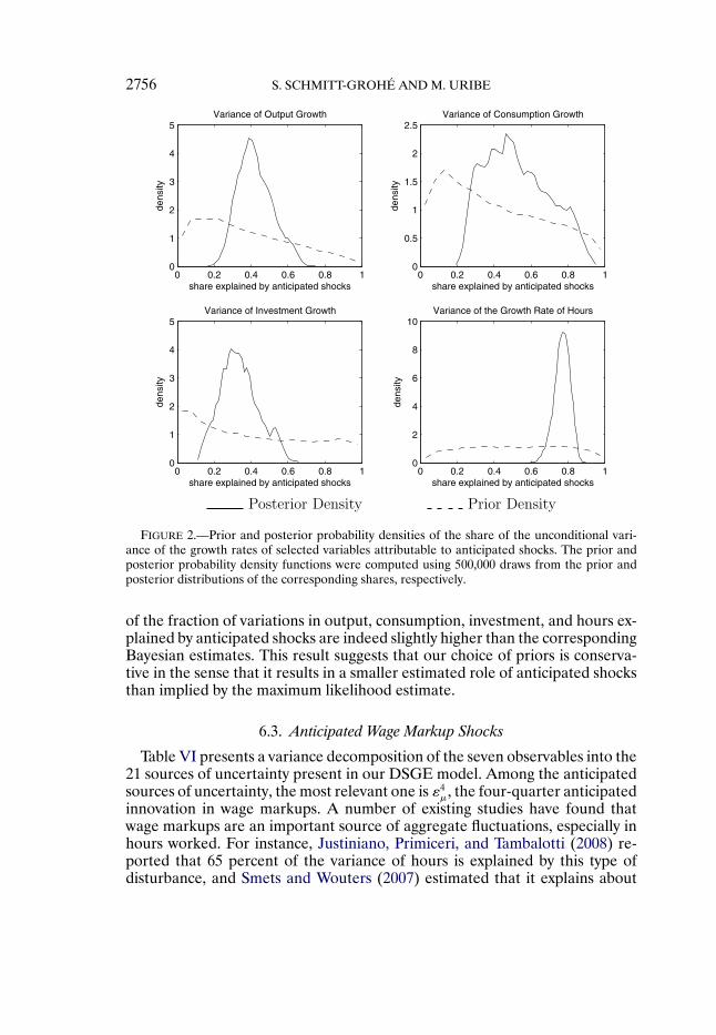
Figure 2 displays the prior and posterior probability density functions ofthe share of the variance of output growth, consumption growth, investmentgrowth, and hours growth accounted for by anticipated shocks in our estimatedmodel. It is evident from this figure that our choice of prior distributions forthe standard deviations of the underlying anticipated and unanticipated dis-turbances delivers highly dispersed prior distributions for the share of varianceaccounted for by anticipated shocks. By contrast, the corresponding posteriordistributions are concentrated around their respective means. This is particu-larly the case for the growth rates of hours worked, output, and investment.The figure demonstrates that our finding of a sizable fraction of aggregatevolatility being explained by anticipated shocks is not an artifact of the assumedpriors.
6.2. Maximum Likelihood Estimate
To further convey the notion that our findings on the importance of antici-pated shocks are not driven by the assumed underlying prior distributions, wepresent in panel 3 of Table V variance decompositions based on a classical max-imum likelihood estimation of the model. The maximum likelihood estimates
2756 S. SCHMITT-GROHÉ AND M. URIBE
FIGURE 2.—Prior and posterior probability densities of the share of the unconditional vari-ance of the growth rates of selected variables attributable to anticipated shocks. The prior andposterior probability density functions were computed using 500,000 draws from the prior andposterior distributions of the corresponding shares, respectively.
of the fraction of variations in output, consumption, investment, and hours ex-plained by anticipated shocks are indeed slightly higher than the correspondingBayesian estimates. This result suggests that our choice of priors is conserva-tive in the sense that it results in a smaller estimated role of anticipated shocksthan implied by the maximum likelihood estimate.
6.3. Anticipated Wage Markup Shocks
Table VI presents a variance decomposition of the seven observables into the21 sources of uncertainty present in our DSGE model. Among the anticipatedsources of uncertainty, the most relevant one is ε4
μ, the four-quarter anticipatedinnovation in wage markups. A number of existing studies have found thatwage markups are an important source of aggregate fluctuations, especially inhours worked. For instance, Justiniano, Primiceri, and Tambalotti (2008) re-ported that 65 percent of the variance of hours is explained by this type ofdisturbance, and Smets and Wouters (2007) estimated that it explains about

WHAT’S NEWS IN BUSINESS CYCLES 2757
TABLE VI
VARIANCE DECOMPOSITIONa
Innovation Y C I h G TFP A
Stationary Neutral Tech. Shock (zt)ε0z 11 3 13 13 0 71 0ε4z 1 0 1 1 0 4 0ε8z 0 0 0 1 0 3 0
Nonstationary Neutral Tech. Shock (μxt )ε0μx 14 9 7 2 4 17 0ε4μx 1 1 0 1 0 2 0ε8μx 1 1 0 1 1 2 0
Stationary Investment-Specific Tech. Shock (zIt )ε0zI
21 1 44 3 0 0 0ε4zI
1 0 4 0 0 0 0ε8zI
6 1 15 2 0 0 0
Nonstationary Investment-Specific Tech. Shock (μat )ε0μa 0 0 0 0 0 0 40ε4μa 0 0 0 0 0 0 30ε8μa 0 0 0 0 0 0 30
Government Spending Shock (gt)ε0g 3 0 0 1 37 0 0ε4g 4 0 0 1 35 0 0ε8g 2 0 0 1 23 0 0
Preference Shock (ζt)ε0ζ 8 34 1 2 0 0 0ε4ζ 4 14 0 1 0 0 0ε8ζ 4 17 0 1 0 0 0
Wage-Markup Shock (μt)ε0μ 0 0 0 2 0 0 0ε4μ 16 17 11 62 0 0 0ε8μ 1 1 1 5 0 0 0
aFigures are in percent and correspond to the mean of 500,000 draws from the posterior distribution of the variancedecomposition. The columns labeled Y , C , I, h, G, TFP, and A refer, respectively, to the growth rates of output,private consumption, investment, hours, government consumption, total factor productivity, and the relative price ofinvestment.
half of the forty-quarter ahead forecasting error variance of output. Our find-ings are consistent with these results. Wage-markup shocks explain 69 percentof the unconditional variance of hours growth and 17 percent of the uncondi-tional variance of output growth. However, our results depart from the exist-ing literature in that we find that virtually the totality of movements in hoursand output due to wage-markup shocks is attributable to its anticipated com-

2758 S. SCHMITT-GROHÉ AND M. URIBE
ponent. Specifically, we estimate that four-quarter anticipated markup shocksexplain 62 percent of the variance of employment growth and 16 percent ofthe variance of output growth. By contrast, unanticipated variations in wagemarkups are estimated to have a negligible role in generating movements inhours and other indicators of aggregate activity. A possible interpretation ofanticipated wage-markup shocks is that they represent expected outcomes ofwage and benefit negotiations between employers and workers that are de-cided in the present but implemented with a lag.
The reason anticipated wage-markup shocks are favored by our data sampleis that they help account for the observed regularity that output and the maincomponents of aggregate demand (consumption and investment spending) alllead employment. We documented this pattern in the Supplemental Material(Schmitt-Grohé and Uribe (2012), Sec. A.5). There, we also showed that theDSGE model’s ability to capture this pattern diminishes when we shut off thefour-period anticipated markup shock. The intuition behind this result is thatan increase in expected wage markups represents an anticipated adverse cost-push shock to the economy. It induces firms to immediately cut spending ininvestment goods and to lower capacity utilization. It also induces householdsto adjust consumption downward upon the news, as they anticipate a declinein income. By contrast, labor supply does not adjust much on impact. This isbecause our estimated wealth elasticity of labor supply, governed by the pa-rameter γ, is close to zero. Instead, the response of hours is delayed and takesplace mostly once the markup shock is realized. In this way, the model cap-tures the observed lagging behavior of employment relative to output and thecomponents of aggregate demand.
6.4. Anticipated Government Spending Shocks
Our estimation results shed light on the debate on whether governmentspending shocks are mostly anticipated or unanticipated. In our model, gov-ernment spending, like all other exogenous variables considered, is subject tounanticipated innovations as well as to innovations that are anticipated fouror eight quarters. In the VAR literature that uses the narrative approach tothe identification of government spending shocks, for example, Ramey andShapiro (1998), a central argument is that changes in government spendingare known several quarters before they result in actual increases in spend-ing. By contrast, Blanchard and Perotti (2002) identified government spendingshocks that are by construction unanticipated. Mountford and Uhlig (2009)applied the sign restriction methodology due to Uhlig (2005) to identify antici-pated and unanticipated fiscal shocks in vector autoregressions. Our proposedmodel-based methodology allows us to jointly evaluate the relative importanceof both types of government spending shocks. Table VI shows that 60 percent ofthe variance of government spending is due to anticipated shocks and 40 per-cent is due to unanticipated shocks. Furthermore, the table shows that gov-ernment spending shocks account for close to 10 percent of the variance of
WHAT’S NEWS IN BUSINESS CYCLES 2759
output growth. This magnitude is standard in the literature. A novel insightemerging from our econometric estimation is that two thirds of this fractionis attributable to anticipated innovations and one third to surprise movementsin government spending. This result suggests that the VAR and narrative ap-proaches to estimating the effects of government spending shocks are not mu-tually exclusive, but complementary.
6.5. Investment-Specific Shocks
A growing literature is concerned with the macroeconomic effects ofinvestment-specific shocks. Our economic environment embeds two such dis-turbances: At and zIt . The shock At affects the rate of transformation of con-sumption goods into investment goods, whereas zIt affects the rate of trans-formation of investment goods into installed capital. Table VI shows that At
is estimated to play no role in generating economic fluctuations. This result isin sharp contrast with that obtained by Justiniano, Primiceri, and Tambalotti(2008), whose estimation assigns a central role to this disturbance. The reasonfor this discrepancy is that our estimation includes the relative price of invest-ment as an observable, whereas the estimation in Justiniano et al. does not. Asmentioned earlier, the relative price of investment is linearly linked toAt . Thenegligible role ofAt in our estimation reflects the fact that the observed volatil-ity of the relative price of investment is low. If we were to eliminate the priceof investment from the set of observables, At would emerge as an importantdriver of aggregate fluctuations, but at the cost of an implied volatility of therelative price of investment several times larger than its observed counterpart.
On the other hand, the investment-specific shock zIt is estimated to explain asignificant fraction of variation in output (28 percent) and investment (63 per-cent). This result is consistent with those reported in Justiniano, Primiceri, andTambalotti (2011). A novel result emerging from our investigation is that a sub-stantial fraction of the contribution of zIt to aggregate volatility (about 30 per-cent) is due to its anticipated components.
6.6. No Anticipation in TFP Shocks
Finally, in line with many existing studies, we find that neutral technologyshocks explain a sizable fraction of the variance of output growth, about 30 per-cent. However, we find that all of this contribution stems from the unantici-pated component of TFP. The minor role assigned to anticipated neutral pro-ductivity shocks is a consequence of the fact that, in our formulation, this typeof shock competes with a variety of other shocks. In the Supplemental Material(Schmitt-Grohé and Uribe (2012), Sec. A.7), we showed that, in the context ofa more parsimonious shock specification that allows only for productivity andgovernment spending shocks, the anticipated component of neutral technologyshocks plays a major role in driving business cycles.

2760 S. SCHMITT-GROHÉ AND M. URIBE
6.7. The Anticipated Component of Hodrick–Prescott-Filtered Business Cycles
Panel 5 of Table V shows that the role of anticipated shocks is also estimatedto be prominent when one measures the business-cycle component of a timeseries by using the Hodrick–Prescott filter. We perform this exercise as follows.(1) We draw a realization of the vector of estimated parametersΘ from its pos-terior or prior distribution, depending on whether we are computing posterioror prior share densities. (2) Then, allowing only one innovation to be activeat a time, we generate artificial time series of the logarithmic levels of out-put, consumption, investment, and hours of length 500 quarters. (Log-levelsare obtained by accumulating growth rates.) At this point, our procedure hasdecomposed each endogenous variable of interest (i.e., output, consumption,investment, and hours) into 21 independent time series corresponding to the21 innovations included in our model. (3) We apply the Hodrick–Prescott filterto the last 207 observations—the length of our actual data sample—of each ofthe 21 independent components using a smoothing parameter value of 1600.(4) For each variable of interest (output, consumption, investment, and hours),we compute the ratio of the sum of the variances of its 14 components associ-ated with anticipated shocks to the sum of the variances of all of its 21 compo-nents. This ratio provides the share of the variance attributable to anticipatedshocks for each endogenous variable considered. (5) We repeat steps (1)–(4)500,000 times and report the median shares as well as the 5th and 95th per-centiles. This procedure takes into account both parameter and finite-sampleuncertainty.
We find that the median share of predicted variances explained by antici-pated shocks at business-cycle frequencies, as defined by the HP filter, is higherthan those obtained using growth rates. This is particularly the case for invest-ment, for which the share explained by anticipated shocks rises from 33 per-cent when the cycle is described by unconditional second moments of first-differenced variables, to 47 percent when the cycle is measured using simu-lated, HP-filtered time series. Overall, anticipated shocks explain between 46and 84 percent of the variances of the four macroeconomic indicators con-sidered. These results suggest that the importance of anticipated shocks inaccounting for variations in business fluctuations is robust to detrending thepredicted time series using growth rates or using the Hodrick–Prescott filter.
6.8. Incorporating Data on Stock Prices
The empirical literature on anticipated shocks has emphasized the role ofstock prices in capturing information about future expected changes in eco-nomic fundamentals. Beaudry and Portier (2006), for instance, used observa-tions on stock prices to identify anticipated permanent changes in total factorproductivity. The reason stock prices are believed to be informative about an-ticipated changes in fundamentals is that they are typically considered moreflexible than other nominal and real aggregate variables often included in the

WHAT’S NEWS IN BUSINESS CYCLES 2761
econometric estimation of macroeconomic models. Real variables, such as con-sumption, investment, and employment, are believed to be costly to adjust inthe short run due to the presence of habit formation, time to build, and hir-ing and firing costs. At the same time, the adjustment of product and factorprices is assumed to be hindered by the presence of price rigidities. With thismotivation in mind, we reestimate the model, including in the set of observ-ables the growth rate of the real per capita value of the stock market as mea-sured by the S&P500 Index. In the theoretical model, we associate this variablewith the value of the firm at the beginning of the period, V F
t , defined in Sec-tion 3. Panel 4 of Table V displays the result of this estimation regarding theimportance of anticipated shocks. As expected, when stock prices are includedin the set of observables, the model attributes a larger fraction of business-cycle fluctuations to anticipated shocks. For the four variables considered inthe table, the median share of their unconditional variance explained by an-ticipated shocks ranges from 55 to 82 percent when stock prices are includedin the estimation. Moreover, the posterior distributions of the shares of vari-ances explained by anticipated shocks are more concentrated around their me-dians, pointing more clearly to their importance. The reason we decided notto include stock prices in our baseline estimation is twofold. First, the existingrelated model-based literature on the sources of business cycles typically doesnot include observations on stock prices in estimation (e.g., Smets and Wouters(2007), Justiniano, Primiceri, and Tambalotti (2011)). Excluding stock pricesfrom the baseline estimation facilitates comparison with this literature. Sec-ond, and perhaps more importantly, as is well known, the neoclassical modeldoes not provide a fully adequate explanation of asset price movements.
7. CONCLUSION
In this paper, we perform classical maximum likelihood and Bayesian esti-mation of a dynamic general equilibrium model to assess the importance ofanticipated and unanticipated shocks as sources of macroeconomic fluctua-tions.
Our identification methodology represents a fundamental departure fromVAR-based approaches to the identification of anticipated shocks, for it ex-ploits the fact that, in theoretical environments in which agents are forwardlooking, endogenous variables, such as output, consumption, investment, andemployment, react to anticipated changes in fundamentals, whereas the funda-mentals themselves do not. Moreover, the fact that economic agents’ responsesto future changes in economic fundamentals depend on how far into the fu-ture the change is expected to occur, allows our empirical strategy to identifyhorizon-specific anticipated shocks.
Our central finding is that, in the context of our model, about half of thevariance of the growth rates of output, consumption, investment, and hours isattributable to anticipated disturbances. This result stands in sharp contrast to
2762 S. SCHMITT-GROHÉ AND M. URIBE
those in the existing literature on the sources of business cycles, which implic-itly assumes that the totality of aggregate fluctuations is due to unanticipatedchanges in economic fundamentals.
APPENDIX: DATA SOURCES
The time series used to construct the seven observable variables used in theestimation are:
1. Real Gross Domestic Product, BEA, NIPA table 1.1.6, line 1, billionsof chained 2000 dollars seasonally adjusted at annual rate. Downloaded fromwww.bea.gov.
2. Gross Domestic Product, BEA NIPA table 1.1.5, line 1, billions of dol-lars, seasonally adjusted at annual rates.
3. Personal Consumption Expenditure on Nondurable Goods, BEA, NIPAtable 1.1.5, line 4, billions of dollars, seasonally adjusted at annual rate. Down-loaded from www.bea.gov.
4. Personal Consumption Expenditure on Services, BEA NIPA table 1.1.5,line 5, billions of dollars, seasonally adjusted at annual rate. Downloaded fromwww.bea.gov.
5. Gross Private Domestic Investment, Fixed Investment, Nonresidential,BEA NIPA table 1.1.5, line 8, billions of dollars, seasonally adjusted at annualrate. Downloaded from www.bea.gov.
6. Gross Private Domestic Investment, Fixed Investment, Residential,BEA NIPA table 1.1.5, line 11, billions of dollars, seasonally adjusted at an-nual rate. Downloaded from www.bea.gov.
7. Government Consumption Expenditure, BEA NIPA table 3.9.5, line 2,billions of dollars, seasonally adjusted at annual rate. Downloaded fromwww.bea.gov.
8. Government Gross Investment, BEA NIPA table 3.9.5, line 3, billions ofdollars, seasonally adjusted at annual rate. Downloaded from www.bea.gov.
9. Civilian Noninstitutional Population Over 16, BLS LNU00000000Q.Downloaded from www.bls.gov.
10. Nonfarm Business Hours Worked, BLS, PRS85006033, seasonally ad-justed, index 1992 = 100. Downloaded from www.bls.gov.
11. GDP Deflator = (2)/(1).12. Real Per Capita GDP = (1)/(9).13. Real Per Capita Consumption = [(3)+ (4)]/(11)/(9).14. Real Per Capita Investment = [(5)+ (6)]/(9)/(11).15. Real Per Capita Government Expenditure = [(7)+ (8)]/(9)/(11).16. Per Capita Hours = (10)/(9).17. Relative Price of Investment: Authors’ calculation following the method-
ology proposed in Fisher (2006). An appendix detailing the procedure used inthe construction of this series is available from the authors upon request.

WHAT’S NEWS IN BUSINESS CYCLES 2763
18. Total factor productivity in the non-farm business sector adjusted forcapital capacity utilization. This series is taken from Beaudry and Lucke(2009).
REFERENCES
AN, S., AND F. SCHORFHEIDE (2007): “Bayesian Analysis of DSGE Models,” Econometric Re-views, 26, 113–172. [2748]
BARRO, R., AND R. G. KING (1984): “Time Separable Preferences and International SubstitutionModels of Business Cycles,” Quarterly Journal of Economics, 99, 817–839. [2734]
BEAUDRY, P., AND B. LUCKE (2009): “Letting Different Views About Business Cycles Compete,”in NBER Macro Annual. Chicago, IL: University of Chicago Press. [2763]
BEAUDRY, P., AND F. PORTIER (2006): “Stock Prices, News, and Economic Fluctuations,” Ameri-can Economic Review, 96, 1293–1307. [2735,2760]
BLANCHARD, O., AND R. PEROTTI (2002): “An Empirical Characterization of the Dynamic Ef-fects of Changes in Government Spending and Taxes on Output,” Quarterly Journal of Eco-nomics, 117, 1329–1368. [2758]
CHERNOZHUKOV, V., AND H. HONG (2003): “An MCMC Approach to Classical Estimation,”Journal of Econometrics, 115, 293–346. [2738,2753]
CHRISTIANO, L. J., M. EICHENBAUM, AND C. L. EVANS (2005): “Nominal Rigidities and theDynamic Effects of a Shock to Monetary Policy,” Journal of Political Economy, 113, 1–45. [2740]
COCHRANE, J. (1994): “Shocks,” Carnegie–Rochester Conference Series on Public Policy, 41,295–364. [2735]
DAVIS, J. M. (2007): “News and the Term Structure in General Equilibrium,” UnpublishedManuscript, Northwestern University. [2735]
FISHER, J. D. M. (2006): “The Dynamic Effects of Neutral and Investment-Specific TechnologyShocks,” Journal of Political Economy, 114, 413–451. [2762]
FUJIWARA, I., Y. HIROSE, AND M. SHINTANI (2008): “Can News Be a Major Source of Aggre-gate Fluctuations? A Bayesian DSGE Approach,” IMES Discussion Paper 2008-E-16, Bank ofJapan. [2735]
GREENWOOD, J., Z. HERCOWITZ, AND G. HUFFMAN (1988): “Investment, Capacity Utilization,and the Real Business Cycle,” American Economic Review, 78, 402–417. [2740,2751]
ISKREV, N. (2010): “Local Identification in DSGE Models,” Journal of Monetary Economics, 57,189–210. [2738,2752]
JAIMOVICH, N., AND S. REBELO (2009): “Can News About the Future Drive the Business Cycle?”American Economic Review, 99, 1097–1118. [2734,2739,2742,2747]
JUSTINIANO, A., G. PRIMICERI, AND A. TAMBALOTTI (2008): “Investment Shocks and BusinessCycles,” Unpublished Manuscript, Northwestern University. January 24, 2008 version. [2739,
2748,2756,2759](2011): “Investment Shocks and the Relative Price of Investment,” Review of Economic
Dynamics, 14, 101–121. [2734,2741,2759,2761]LEEPER, E. M., T. B. WALKER, AND S.-C. S. YANG (2008): “Fiscal Foresight and Information
Flows,” Unpublished Manuscript, Indiana University. [2734]MOUNTFORD, A., AND H. UHLIG (2009): “What Are the Effects of Fiscal Policy Shocks?” Journal
of Applied Econometrics, 24, 960–992. [2758]PIGOU, A., (1927): Industrial Fluctuations. London: Macmillan. [2735]RAMEY, V., AND M. D. SHAPIRO (1998): “Costly Capital Reallocation and the Effects of Govern-
ment Spending,” Carnegie–Rochester Conference Series on Public Policy, 48, 145–194. [2758]SCHMITT-GROHÉ, S., AND M. URIBE (2004): “Solving Dynamic General Equilibrium Models Us-
ing a Second-Order Approximation to the Policy Function,” Journal of Economic Dynamics andControl, 28, 755–775. [2747]

2764 S. SCHMITT-GROHÉ AND M. URIBE
(2011): “Business Cycles With a Common Trend in Neutral and Investment-SpecificProductivity,” Review of Economic Dynamics, 14, 122–135. [2741]
(2012): “Supplement to ‘What’s News in Business Cycles’,” Econometrica SupplementalMaterial, 80, http://www.econometricsociety.org/ecta/Supmat/8050_extensions.pdf; http://www.econometricsociety.org/ecta/Supmat/8050_data_and_programs.zip. [2737,2739,2745,2746,
2752,2758,2759]SMETS, F., AND R. WOUTERS (2007): “Shocks and Frictions in US Business Cycles: A Bayesian
DSGE Approach,” American Economic Review, 97, 586–606. [2734,2739,2741,2756,2761]UHLIG, H. (2005): “What Are the Effects of Monetary Policy? Results From an Agnostic Identi-
fication Procedure,” Journal of Monetary Economics, 52, 381–419. [2758]
Dept. of Economics, Columbia University, New York, NY 10027, U.S.A., CEPR,and NBER; [email protected]
andDept. of Economics, Columbia University, New York, NY 10027, U.S.A. and
NBER; [email protected].
Manuscript received August, 2008; final revision received July, 2011.