What would have happened to the ozone layer if ...€¦ · ozone depletion, a failure to regulate...

Atmos. Chem. Phys., 9, 2113–2128, 2009www.atmos-chem-phys.net/9/2113/2009/© Author(s) 2009. This work is distributed underthe Creative Commons Attribution 3.0 License.

AtmosphericChemistry

and Physics

What would have happened to the ozone layer ifchlorofluorocarbons (CFCs) had not been regulated?

P. A. Newman1, L. D. Oman2, A. R. Douglass1, E. L. Fleming3, S. M. Frith 3, M. M. Hurwitz 4, S. R. Kawa1,C. H. Jackman1, N. A. Krotkov 5, E. R. Nash3, J. E. Nielsen3, S. Pawson1, R. S. Stolarski1, and G. J. M. Velders6

1NASA Goddard Space Flight Center, Greenbelt, Maryland, USA2Johns Hopkins University, Baltimore, Maryland, USA3Science Systems and Applications, Inc., Lanham, Maryland, USA4NASA Postdoctoral Program, NASA Goddard Space Flight Center, Greenbelt, Maryland, USA5Goddard Earth Sciences and Technology Center, University of Maryland, Baltimore County, Baltimore, Maryland, USA6Netherlands Environmental Assessment Agency, Bilthoven, The Netherlands

Received: 22 September 2008 – Published in Atmos. Chem. Phys. Discuss.: 10 December 2008Revised: 17 March 2009 – Accepted: 18 March 2009 – Published: 23 March 2009

Abstract. Ozone depletion by chlorofluorocarbons (CFCs)was first proposed by Molina and Rowland in their 1974Nature paper. Since that time, the scientific connection be-tween ozone losses and CFCs and other ozone depletingsubstances (ODSs) has been firmly established with labora-tory measurements, atmospheric observations, and modelingstudies. This science research led to the implementation ofinternational agreements that largely stopped the productionof ODSs. In this study we use a fully-coupled radiation-chemical-dynamical model to simulate a future world whereODSs were never regulated and ODS production grew atan annual rate of 3%. In this “world avoided” simulation,17% of the globally-averaged column ozone is destroyed by2020, and 67% is destroyed by 2065 in comparison to 1980.Large ozone depletions in the polar region become year-round rather than just seasonal as is currently observed in theAntarctic ozone hole. Very large temperature decreases areobserved in response to circulation changes and decreasedshortwave radiation absorption by ozone. Ozone levels inthe tropical lower stratosphere remain constant until about2053 and then collapse to near zero by 2058 as a result ofheterogeneous chemical processes (as currently observed inthe Antarctic ozone hole). The tropical cooling that triggersthe ozone collapse is caused by an increase of the tropicalupwelling. In response to ozone changes, ultraviolet radia-tion increases, more than doubling the erythemal radiation inthe northern summer midlatitudes by 2060.

Correspondence to:P. A. Newman([email protected])

1 Introduction

Molina and Rowland(1974) were the first to propose thatozone could be depleted by the release of chlorofluorocar-bons (CFCs) to the atmosphere. The chemical breakdown ofCFCs and other ozone depleting substances (ODSs) in thestratosphere releases chlorine (Cl) and bromine (Br) atomsthat destroy ozone molecules in catalytic cycles. Ozone de-pletion would result in an increase of biologically harmfulsolar ultraviolet (UV) radiation. Early predictions of ozoneloss were 15–18% if CFCs added 5.5–7.0 ppbv of chlorineto the stratosphere (Hudson and Reed, 1979). Continued sci-entific research led to the writing of a series of reports thatculminated in the first World Meteorological Organization(WMO)/United Nations Environment Program scientific as-sessment of ozone depletion (WMO, 1985). This assessmentprovided the scientific consensus that CFCs and halons poseda serious threat to the ozone layer. In response, the land-mark Montreal Protocol agreement was negotiated in 1987(Sarma and Bankobeza, 2000). This agreement regulated theproduction of chlorofluorocarbons and other ODSs. Since1987, 193 nations have signed the Montreal Protocol. Fiveamendments to the Montreal Protocol have now led to thecessation of the major portions of ODS production aroundthe world. The cumulative levels of chlorine and brominefrom the ODSs are now decreasing in both the troposphere(Montzka et al., 1996) and the stratosphere (Anderson et al.,2000; Froidevaux et al., 2006). The work of Molina andRowland(1974) led to a major reorganization and redirectionof chemical production to substitute compounds, to changesin technologies that traditionally used CFCs, and to the firstinternational agreement on regulation of chemical pollutants.

Published by Copernicus Publications on behalf of the European Geosciences Union.

http://creativecommons.org/licenses/by/3.0/

2114 P. A. Newman et al.: TheWORLD AVOIDED

The regulation of ODSs was based upon the ozone assess-ments that presented the consensus of the science commu-nity. The regulation presupposed that a lack of action wouldlead to severe ozone depletion with consequent severe in-creases of solar UV radiation levels at the Earth’s surface.Because of the successful regulation of ODSs, ozone sciencehas now entered into the accountability phase. There are tworelevant questions in this phase. First, are ODS levels de-creasing and ozone increasing as expected because of theMontreal Protocol regulations? Second, what would havehappened to the atmosphere if no actions had been taken?That is to say, what kind of world was avoided? It is thislatter question that is the focus of the present study.

Two studies have modeled the impact of high levels ofCFCs on ozone. First,Prather et al.(1996) modeled theozone response to continued growth of the ODSs without theMontreal Protocol and its amendments. They hypothesizedthat ODSs continued to grow at “business-as-usual” growthrates from 1974 into the early 21st century. Such ODSgrowth could have resulted from a lack of understanding ofozone depletion, a failure to regulate ODS production, andfurther development of technologies that used CFCs. In theirstudy, ODSs were allowed to grow by approximately 5–7%per year, resulting in a total stratospheric chlorine (Cly) levelof about 9 ppbv by 2002. They used a two-dimensional (2-D, or latitude-altitude) model with projected CFC and halonlevels to calculate a globally-averaged total ozone depletionof 10% by 1999. Second,Morgenstern et al.(2008) used athree-dimensional (3-D, or longitude-latitude-altitude) cou-pled chemistry-climate model (CCM) to simulate the impactof 9 ppbv on the stratosphere in a timeslice or fixed timemode (equivalent to levels of Cly that they estimated wouldhave been reached in about 2030). In their simulation theyfound peak ozone depletions (>35%) in the upper strato-sphere, with additional ozone depletion in both polar regions(>20%).

In addition to the ozone studies,Velders et al.(2007) haverecently investigated the impact of unrestrained growth ofCFCs on climate. They pointed out that because CFCs andother ODSs are also greenhouse gases, the ODSs would haveadded an additional 0.8–1.6 W m−2 of radiative forcing by2010 if the ODSs had continued to grow at 3–7% per yearafter 1974. Hence, the implementation of the Montreal Pro-tocol has limited both ozone depletion and climate change.

Prather et al.(1996) were limited by using a fixed trans-port 2-D model (Jackman et al., 1996) to produce their es-timates of ozone loss. Since this version of the 2-D modeldid not include the feedback among radiative, dynamical,and chemical processes, the model simulations were termi-nated when total ozone depletion reached 10%. Such signifi-cant computed total ozone depletion was assumed to causelarge stratospheric changes, both radiatively and dynami-cally. Models of the stratosphere have greatly improved overthe last decade. 2-D models parameterize longitudinal varia-tions, hence 3-D models better account for longitudinal vari-

ations and more realistically represent the polar latitude dy-namics. State-of-the-art models now have complex feedbackamong the chemical, radiative, and dynamical processes.

Here we employ the Goddard Earth Observing System(GEOS) chemistry-climate model to explore the ozone dis-tributions that might have been without ODS regulations(a “world avoided”), updating and extending the results ofPrather et al.(1996) up to 2065. Because ozone is a ra-diatively active gas in both the ultraviolet and the infrared,the destruction of ozone alters the temperature and the winddistributions, which then affects the transport of ozone andother gases. Further, as temperatures change, ozone lossrates change, producing a feedback that further alters theozone distribution. Hence, a proper simulation of the “worldavoided” requires a CCM with interactive radiation, chem-istry, and dynamics.

This “world avoided” estimate of ozone depletion is per-formed for a few basic reasons. First, scientists predictedmassive ozone losses, actions were taken, and these losseshave not occurred. Hence, do the state-of-the-art models ac-tually predict the large losses that were hypothesized in the1980s? Second, such model estimates give an indication ofthe unforeseen impacts of large ozone losses on the chem-istry and climate of the stratosphere. Such extreme simula-tions are useful for evaluating theoretical expectations of dy-namics and chemistry (e.g., how does the tropopause changeif the ozone layer is destroyed?). Third, a transient simu-lation provides an ensemble of total chlorine and brominevalues and their associated ozone losses, from small chlo-rine values in the 1960s to high chlorine values in the 2060s.Because we cannot actually predict how large CFC and otherODS concentrations might have become, this simulation pro-vides a large range of CFC levels from which to choose. Fi-nally, and most importantly, this type of estimate providesa quantitative baseline for assessing the impact of interna-tional agreements on ozone, UV radiation impacts, and cli-mate change. The acknowledged success of the MontrealProtocol in the present is best measured against what mighthave been without that agreement.

The scope of this study is limited to describing the verylarge ozone losses and the subsequent rise of ultraviolet (UV)levels. We only include highlights of the radiative, chem-ical, and dynamical effects in the stratosphere. The largeCFC perturbations used here lead to large chemical ozonelosses and large dynamical changes that lead to large ozonechanges. In this study, we have not attempted to separatethese chemical and dynamical effects, but refer to them to-gether as ozone losses. There are eight sections includingthe introduction. Section2 describes the experiment withsubsections on the model and the details of the simulations.Section3 describes the evolution of halogens in the modelexperiments. Section4 describes the evolution and distri-butions of ozone. Sections5 and6 discuss some importantaspects of the chemistry and dynamics, respectively. Sec-tion 7 provides estimates of surface ultraviolet levels. The

Atmos. Chem. Phys., 9, 2113–2128, 2009 www.atmos-chem-phys.net/9/2113/2009/

P. A. Newman et al.: TheWORLD AVOIDED 2115

final section provides a summary and discussion of some im-portant aspects of this “world avoided” scenario.

2 Experiment

The model simulations use the GEOSCCM, which is de-scribed in detail byPawson et al.(2008).

2.1 Model description

The model has a horizontal resolution of 2◦ latitude by 2.5◦

longitude with 55 vertical levels up to 0.01 hPa (80 km).The dynamical time step is 7.5 min. The model uses aflux-form semi-Lagrangian dynamical core (Lin, 2004) anda mountain-forced gravity-wave drag scheme with a waveforcing for non-zero phase speeds (Garcia and Boville, 1994;Kiehl et al., 1998). The sub-grid moisture physics and radi-ation are adapted fromKiehl et al. (1998), as described byBosilovich et al.(2005). The model does not include ei-ther an internally generated or a forced quasi-biennial os-cillation. The photochemistry code is based on the familyapproach, as described byDouglass and Kawa(1999) anduses the chemical kinetics fromSander et al.(2003). Tro-pospheric ozone is relaxed to a climatology (Logan, 1999)with a 5-day time scale. A total of 35 trace gases are trans-ported in the model. Gases with surface sources are specifiedas mixing ratios in the lowest model layer (e.g., “greenhousegases” such as carbon dioxide (CO2) and “ozone-depletinggases” such as CFC-11. The coupling between the chemicaland physical state of the atmosphere occurs directly throughthe GCM’s radiation code. The model-simulated water va-por (H2O), CO2, ozone (O3), methane (CH4), nitrous ox-ide (N2O), CFC-11, CFC-12, and HCFC-22 are used in theradiation computations. The same A1b IntergovernmentalPanel on Climate Change (IPCC) greenhouse gas scenario(Table II.2.1, ISAM model reference, and Tables II.2.2 andII.2.3 fromHoughton et al., 2001) is used for CO2, CH4, andN2O in all of our simulations.

Processes involving polar stratospheric clouds (PSCs) usean update of the parameterization described byConsidineet al.(2000). In this approach PSC particles composed of ni-tric acid trihydrate (NAT) or water ice form instantaneouslywhen the ambient mixing ratios of nitric acid (HNO3) or H2Oare above the respective saturation mixing ratio, which is afunction of temperature and pressure (and H2O mixing ratiofor NAT). No supersaturation is required for PSC formationin this simulation. PSC reactive surface area is calculatedfrom the amount of condensed mass assuming a prescribedparticle number concentration for either ice or NAT. Particlesedimentation follows from a log-normal size distribution.In the simulation of the “world avoided”, both NAT and icesedimentation directly redistribute HNO3 and H2O verticallybetween grid boxes; no separate dehydration parameter isneeded as inConsidine et al.(2000). Heterogeneous reaction

efficiencies (sticking coefficient) are calculated for the appro-priate surface type: liquid sulfate, NAT, or ice, as inKawaet al. (1997) updated toSander et al.(2003). The sulfateaerosol surface area is based upon Stratospheric Aerosol andGas Experiment (SAGE) observations, and is specified as aclimatological zonal mean varying as a function of month,altitude, and latitude for non-volcanically influenced periods(Chipperfield et al., 2003).

GEOSCCM has been compared to observations and othermodels and does very well in reproducing past climate andkey transport processes (Eyring et al., 2006; Stolarski et al.,2006; Pawson et al., 2008; Oman et al., 2009). Pawson et al.(2008) showed good agreement between the ozone simula-tions and observations, but noted a slightly high total ozonebias and a too cold and long-lived Antarctic vortex. Cly hasbeen estimated from observations byLary et al.(2007), andshows good agreement with the GEOSCCM values (Eyringet al., 2007). In addition, hydrochloric acid (HCl) fromGEOSCCM has also been compared to observations andshows excellent agreement (Eyring et al., 2006). Predic-tions from the GEOSCCM have been compared to othermodel predictions (Eyring et al., 2007), showing good gen-eral agreement with other CCMs. These comparisons of bothozone and chlorine observations give us high confidence inthe GEOSCCM projections.

2.2 Model simulations

There are four simulations used in this study: a “referencepast”, a “reference future”, a “fixed chlorine” (with chlorinelevels fixed at the 1960 level), and the “WORLD AVOIDED”.Table 1 summarizes the four simulations. Figures in thisstudy that compare the simulations use color to distinguishbetween them, using blue for thereference past, red for thereference future, green for thefixed chlorine, and black fortheWORLD AVOIDED. The first three simulations have beendescribed byPawson et al.(2008) andOman et al.(2009).Thereference pastandreference futuresimulations have alsobeen described byEyring et al. (2006) and Eyring et al.(2007), respectively.

The reference pastsimulation is an attempt to simulatethe past observations of the atmosphere. Hence this simula-tion is forced by the observed ODSs at the surface (Montzkaet al., 2003), and uses the observed sea surface temperatures(SSTs) and ice distribution (Rayner et al., 2003). Therefer-ence futureis an attempt to simulate the future using our bestguesses for future ODSs (Montzka et al., 2003) and SSTs.There are tworeference futuresimulations shown herein. Allof the reference futureplots versus time use the same simu-lation shown byEyring et al.(2007) that was forced with theHadGEM1 SSTs. All of the zonal mean difference plots usea reference future simulation that is forced with the NationalCenter for Atmospheric Research (NCAR) Community Cli-mate System Model version 3 (CCSM3) SSTs (Collins et al.,2006). This second reference future simulation (B in Table1)

www.atmos-chem-phys.net/9/2113/2009/ Atmos. Chem. Phys., 9, 2113–2128, 2009


Table 1. GEOSCCM simulations description

Simulation Year range ODS scenario Prescribed SSTs

Reference past 1950–2004 Aba Observations: HadISST1b

Reference future 1996–2099 Aba A: HadGEM1c

2000–2099 B: NCAR CCSM3 SRESA1BFixed chlorine 1960–2100 Aba, fixed to 1960 1960–2000: Observations: HadISST1b

2001–2100: NCAR CCSM3 PCMDIWORLD AVOIDED 1974–2065 +3% per year 1974–2049: NCAR CCSM2 SRESA1B

2050–2065: NCAR CCSM3 SRESA1B

a Montzka et al.(2003)b Rayner et al.(2003)c Johns et al.(2006)

is used because the SSTs are consistent with theWORLDAVOIDEDsimulation in the period from 2050 to 2065. Thedifferences between these tworeference futuresimulationsare quite small in the stratosphere.

The WORLD AVOIDEDsimulation extends from 1974through 2065. This simulation is driven by one of the mixingratio scenarios established inVelders et al.(2007). The ODSestimates are based upon a scenario (their MR74) whereinproduction of the CFC-11, CFC-12, CFC-113, CFC-114,CFC-115, carbon tetrachloride, methyl chloroform, HCFC-22, HCFC-142b, halon 1301, and methyl bromide increasesannually at 3% per year beginning in 1974. In this scenario,there was no early warning of the danger of CFCs as actuallyoccurred because ofMolina and Rowland(1974). The 3%per year production growth is lower than the observed growthof 12–17% in CFC production in the period up to 1974. Thesurface total chlorine reaches a level of 9 ppbv in 2012. Incontrast, the CFC growth used inPrather et al.(1996) wasapproximately 7% and Cly reached a level of 9 ppbv in about2002.Morgenstern et al.(2008) compared two fixed Cly lev-els of 3.5 ppbv and 9 ppbv in their timeslice simulation. Inour WORLD AVOIDEDsimulation, the upper stratosphericCly reaches 9 ppbv in about 2019.

Reliable estimates of surface temperature changes canonly be made using coupled atmosphere-ocean general cir-culation models (AOGCMs) (Houghton et al., 1990). In ourCCM we attempt to overcome this problem by using SSTsthat are consistent with increasing greenhouse gases. TheSSTs and sea ice used in theWORLD AVOIDEDsimula-tion are derived from two integrations of the NCAR Commu-nity Climate System Model, from the version 2 (CCSM2) for1974–2049 and from the CCSM3 for 2050–2065. The latteris from an IPCC AR4 integration, but both are consistent withthe IPCC A1b scenario growth of greenhouse gases. A lim-itation of this prescribed SST approach is that it is inconsis-tent with the growth of the ODSs in ourWORLD AVOIDEDsimulation. Since ODSs are also greenhouse gases, they in-troduce a direct radiative forcing in the atmosphere (less soin the stratosphere since CFCs are destroyed there). Ozone is

also a greenhouse gas, so stratospheric ozone changes alsoprovide a radiative forcing of the troposphere. The pre-scribed SST used herein acts as a thermal sink, constrainingthe troposphere to evolve in parallel with A1b greenhousegas growth rather than with the additional radiative forcingfrom the higher levels of CFCs. Assuming a climate sen-sitivity parameter of 0.5 K(W m−2)−1 (Ramanathan et al.,1985), the additional CFCs would contribute a surface warm-ing of very roughly 0.25 K by 2010 following theVelderset al.(2007) estimates of the CFC induced radiative forcing.Hence, theWORLD AVOIDEDtroposphere and oceans aretoo cold compared with what would develop for the samescenario using an AOGCM. Furthermore, the extreme UVlevels simulated here would also impact tropospheric chem-istry, tropospheric ozone radiative forcing, and biogeochem-ical processes. The GEOSCCM model is a stratosphere-onlychemistry model that uses a climatological distribution ofozone in the troposphere. While tropospheric reductions ofozone are evident in the model’s ozone field, these reduc-tions are solely a result of the advection of low ozone fromthe stratosphere.

We also simulated theWORLD AVOIDEDusing a coupledchemistry 2-D model with theVelders et al.(2007) MR74scenario. This 2-D model is an updated version of that usedby Rosenfield et al.(2002). This is also an improvementover the 2-D model ofPrather et al.(1996) that utilized pre-scribed transport fields that did not interact with the evolu-tion of the chemical fields. Our newer model has fully in-teractive chemistry, radiation, and dynamics, and includes aparameterization of eddy effects that interact with the meancirculation (Garcia, 1991). While the dynamics, chemistry,and physics of the GEOSCCM and the 2-D model are verydistinct, the newer 2-D model results are in good quantita-tive agreement with the results herein from the GEOSCCMWORLD AVOIDEDsimulation.



Fig. 1. EESC versus year for theWORLD AVOIDEDas globally-averaged from the model’s inorganic chlorine and bromine at4.5 hPa (thick black line). The magenta lines show scenarios fromthe Montreal Protocol, the London Amendments, and the Copen-hagen Amendments. The red line indicates the estimate of ODSevolution in the Ab scenario and the blue line indicates observa-tionally based EESC (Montzka et al., 2003). The green line showsthe fixed level of 1960 chlorine (1.2 ppbv). EECl for theWORLDAVOIDED is shown as the dark purple line.

3 Atmospheric halogens

In this WORLD AVOIDEDsimulation, stratospheric ODSlevels increase rapidly after 2000. Figure1 shows the equiv-alent effective chlorine (EECl) fromVelders et al.(2007)(purple line) that is used as the surface mixing ratio bound-ary condition in theWORLD AVOIDEDsimulation. ThisEECl is estimated by totaling all of the inorganic chlorineand bromine separately and then adding them with the inor-ganic bromine multiplied by a factor of 60 to account for thegreater efficiency of bromine for ozone destruction.

The effective equivalent stratospheric chlorine (EESC)(thick black line) is calculated in Fig.1 from the model out-put by summing the globally-averaged Cly and total strato-spheric bromine (Bry) at 4.5 hPa with a Bry scaling factorof 60. TheWORLD AVOIDEDEESC is somewhat uncer-tain because the scaling factor of 60 used for the estimateof the Bry contribution will change at very high concentra-tions of Cly (Danilin et al., 1996). We also theoretically es-timate EESC followingNewman et al.(2007), using the sur-face mixing ratio estimates and fractional release rates foreach species, and an age spectrum with a 6-year mean age.This theoretical EESC (not shown here) overlaps the modelEESC, giving us good confidence in these model estimates.In addition, Froidevaux et al.(2006) estimated total chlo-rine from Microwave Limb Sounder HCl observations in theupper stratosphere as approximately 3.6 ppbv in 2006 witha slow decrease of about 0.8% per year. Thereference fu-

Fig. 2. Annual average global ozone for theWORLD AVOIDED(solid black),reference future(red),fixed chlorine(green), andref-erence past(blue) simulations. The curves are smoothed with aGaussian filter with a half-amplitude response of 20 years, exceptfor theWORLD AVOIDED, which is unsmoothed. The dashed lineshows the 2-D coupled model simulation of the “world avoided”.The thin horizontal lines indicate the 220-DU level (the level usu-ally indicating the areal extent of the Antarctic ozone hole) andthe 310-DU level (the 1980 global value). The inset shows theWORLD AVOIDEDtotal ozone plotted against global annually-averaged EESC at 4.5 hPa from Fig.1.

ture simulation has a peak in total chlorine of 3.4 ppbv witha decrease that matches the observed 0.8% per year, againgiving us good confidence in our ability to simulate chlo-rine levels. The time lag between the model EESC and theEECl is accounted for by the transit time from the Earth’ssurface to the upper stratosphere (≈4–6 years). The EESCtheoretical estimates (again followingNewman et al., 2007)are shown for the Montreal Protocol, the London Amend-ments, the Copenhagen Amendments, observations, and sce-nario Ab (Montzka et al., 2003). The current A1 scenario(Daniel et al., 2007) is not shown here, but nearly overlapsthe Ab scenario in Fig.1.

The natural level of EESC is estimated to be approxi-mately 1.2 ppbv (noted at the left in Fig.1). In the Ab sce-nario, the EESC reached a peak level of about 4.3 ppbv inapproximately 2002. TheWORLD AVOIDEDscenario hasEESC increasing to 11.5 ppbv by 2020 and 29.6 ppbv by2050. In contrast, scenario Ab has EESC falling to 3.8 ppbvin 2020 and 2.8 ppbv by 2050.

4 Ozone

Figure 2 displays the global annual average total ozonelevels from the four simulations. Total ozone falls fromabout 315 DU in 1974 to about 110 DU in 2065 in theWORLD AVOIDEDsimulation. Approximately 27 DU ofthis annually-averaged total ozone is in the troposphere over



the entire period. A value of less than 220 DU is nominallyused to estimate the location and areal extent of the Antarc-tic ozone hole. The global annual average passes 220 DUshortly before 2040.

Figure 2 also shows theWORLD AVOIDEDsimulation(with the same ODS scenario) using the coupled chemistry2-D model (dashed line). The 2-D model shows less ozoneprior to 2000. However, in spite of the large differences inthese model implementations (e.g., 2-D vs. 3-D, chemicalschemes, dynamical parameterizations, etc.), the two modelsshow very good agreement after 2000, which provides confi-dence in the magnitudes of the ozone losses.

This good agreement between the 2-D and 3-D models isnot surprising in light of previous studies, which showed thatthe zonally-averaged stratospheric ozone and tracer fieldssimulated by 3-D models were well represented by self-consistent 2-D model simulations on time scales of 30 daysor longer (e.g.,Plumb and Mahlman, 1987; Yudin et al.,2000). Also, our previous work has shown that a 2-D modelframework can successfully reproduce many of the transport-sensitive features seen in a variety of stratospheric ozone andtracer observations (Fleming et al., 1999). The good 2-D/3-D model agreement also illustrates that the propagation andbreakdown of planetary waves in the stratosphere, and therelated interactions with the zonal mean flow, are well rep-resented by the linearized planetary wave parameterizationused in our 2-D model (Garcia, 1991), even in this highlyperturbedWORLD AVOIDEDscenario.

The sensitivity of total ozone to chlorine is roughly linearover the time period simulated. The inset to Fig.2 showsthe total ozone plotted against the model EESC. The ozonelevel is linearly anti-correlated with the EESC level. Whilethe temporal tendency in Fig.2 shows an accelerating decline(i.e., the change between 2040 and 2060 is greater than thechange between 2020 and 2040), this is a result of the accel-erating increase of ODSs, rather than a greater sensitivity toODSs.

Substantial reduction of ozone occurs at all latitudes in theWORLD AVOIDEDsimulation. Figure3 shows annually-averaged total ozone for a series of years from all four sim-ulations. The total ozone in 1970 is represented by thefixedchlorine and reference pastsimulations (both have compa-rable EESC levels in 1970, see Fig.1). These simulationsare in reasonable agreement with observations (seePaw-son et al., 2008) with a global total ozone average of about310 DU. Thereference futureandWORLD AVOIDEDsim-ulations show substantial ozone losses by 2000 as ODSs in-crease. This loss trend continues as ODSs increase, such thatglobal total ozone has fallen to a value of about 120 DU by2065 in theWORLD AVOIDEDsimulation. The midlatitudemaximum in both hemispheres has virtually disappeared by2065, and annually-averaged polar values have dropped be-low 100 DU. In addition, this midlatitude maximum slowlyshifts equatorward in both hemispheres. A substantial por-tion of the remaining total column is found in the troposphere

Fig. 3. Annually-averaged total ozone versus latitude for variousyears from theWORLD AVOIDED(black), reference future(red),fixed chlorine(green), andreference past(blue) simulations. Thepole-to-pole area-weighted averages are shown in Fig.2.

(approximately 20 DU in the Antarctic, 24 DU in the Arctic,and 20 DU in the tropics, with a global average troposphericcolumn of 27 DU).

In the WORLD AVOIDEDsimulations polar total ozonealso shows severe losses. Over the Arctic (Fig.4a), ozonedecreases from values near 500 DU in the 1960–1980 periodto less than 100 DU by 2065 (an 80% depletion over approx-imately an 80-year time span). Approximately 24 DU of thisremaining Arctic column is in the troposphere. The inset im-ages show the April monthly averages for 1980, 2020, and2040. In 1980, the large column amounts cover the Arcticregion (values>500 DU). By 2020, a distinct “ozone hole”minimum has developed over the Arctic with a low valuenear the pole that is less than 200 DU. By 2060 values of lessthan 100 DU are found over the Arctic. The positive gradientof ozone between the midlatitudes and the pole seen in 1980has disappeared by 2060.

Over Antarctica (Fig.4b), the October average drops be-low 100 DU in approximately 2025 and continues to slowlydecrease to about 50 DU by 2060. Of this 50 DU, approx-imately 20 DU is found in the troposphere. The inset im-ages show the October averages for 1980, 2020, and 2060.In 1980, a distinct ozone low is seen over Antarctica. By2040, this low has considerably deepened, and by 2060 ex-tremely low values are observed across Antarctica and intomidlatitudes. These October images also show the very largedepletions of ozone in the midlatitude collar region.

Antarctic ozone, at the profile peak (≈50 hPa), reaches100% loss by 2000 (saturation), as observed in ozonesondes(Solomon et al., 2005). This saturation occurs because of thecolder Antarctic temperatures and thereby greater coverageof PSCs and cold sulfate aerosols. The heterogeneous reac-tions on the surfaces of these PSCs and aerosols fully activate



Fig. 4. Total ozone in(a) April for the Arctic and(b) October for theAntarctic for theWORLD AVOIDED(black),reference future(red),fixed chlorine(green), andreference past(blue) simulations. Thecurves are smoothed with a Gaussian filter with a half-amplituderesponse of 20 years, except for theWORLD AVOIDED, which isunsmoothed. The inset false-color images show (a) April and (b)October averages for 1980, 2020, and 2060 with 20-DU color in-crements (see inset scale).

chlorine, leading to massive ozone loss. Hence, in Fig.4b wesee a rapid ozone decline before 2000 with a slower declineafter 2000 as ozone losses expand into the regions above andbelow 50 hPa. In contrast, Arctic total ozone decreases lin-early because saturation effects do not occur (e.g.,Tripathiet al., 2007).

In addition to radical changes in the spring polar columnamount in theWORLD AVOIDEDsimulation, the annual cy-cle of total ozone over the polar regions is also radically al-tered. Figure5 displays the column values versus the day ofthe year over the Arctic (Fig.5a) and the Antarctic (Fig.5b)at 10-year increments from 1980 to 2060, with the additionof 2065. The Arctic (Fig.5a) peak levels in the early years(1980–1990) occur in the springtime. Large depletions in theArctic spring become apparent by the late 1990s, and gradu-ally worsen in later years. As seen in Fig.4a, the April ozone

Fig. 5. Total ozone from theWORLD AVOIDEDsimulation over(a)the Arctic (70◦–90◦ N average) and(b) the Antarctic (70◦–90◦ Saverage) versus day of the year for a selected set of years from 1980to 2065. The years are alternated black and grey for illustrativepurposes. The Arctic values are shifted by 6 months (note the breakbetween 31 December and 1 January) for comparison to the Antarc-tic.

reaches a 220-DU level in about 2030. The observed au-tumn through winter increase of ozone is clearly seen in 1980(Bowman and Krueger, 1985), but by 2020 this has been in-verted to a decrease. A comparison of the 1980 values with2040 reveals a complete phase shift of the annual cycle.

The Antarctic annual cycle (Fig.5b) shows a worsen-ing spring situation. The development of the ozone holeis clearly seen in the spring by comparison of 1980 to the1990 and 2000 curves. The ozone hole continues to worseninto the 21st century with lower values and earlier onsets ofthe minimum value. Also note that the spring-to-summerincrease of ozone has weakened by 2030, thereby creatinga year-round ozone hole. This weak summer increase re-sults from the decreased advection into the Antarctic regionas ozone is depleted in both the upper stratosphere and mid-latitude middle and lower stratosphere. By 2050 the annualcycle of ozone over Antarctica is relatively small because ofthe very strong in situ depletion and the lack of advectiveresupply of ozone to the Antarctic region.



Fig. 6. Percentage total ozone difference between theWORLDAVOIDEDand thereference futuresimulations for a decadal aver-age (2055–2065). The dashed contours are in 20% increments whilecolors are in 10% increments. The magenta line shows theWORLDAVOIDED tropopause. The white lines show the zonal-mean zonalwinds (easterlies are dashed) for theWORLD AVOIDEDsimulation.

The WORLD AVOIDEDsimulation has its largest lossesin two distinct vertical layers: the lower stratosphere (200–30 hPa), and in the upper stratosphere (2 hPa). Since mostof the ozone is found in the lower stratosphere, the lowerstratospheric losses dominate the column losses seen in Fig.2through Fig.5. Figure 6 displays the 2060 difference inannually-averaged ozone losses as a function of altitude andlatitude between theWORLD AVOIDEDand thereferencefuturesimulations. The annually-averaged losses in the 200–30 hPa region of Antarctica exceed 90% in the region extend-ing out to the edge of the polar vortex (the peak of the zonalmean winds is colocated with the polar vortex edge). Arc-tic lower stratospheric annually-averaged losses also exceed90% by 2060. In addition to the polar loss, a large tropicallower stratospheric loss (>70%) is also observed in the 70–30 hPa layer.Morgenstern et al.(2008) showed a very similarpattern of upper stratospheric losses and polar losses in com-parison to ourWORLD AVOIDED2020 to 2000 differences.

Upper stratospheric losses exceed 60% over a large lati-tude width in the 5–0.5 hPa region, with peak losses above70% in the midlatitudes. Middle stratosphere losses aresomewhat less (40–60%) in the 5–3 hPa layer. In additionto the stratospheric losses, ozone losses extend into the tro-posphere (the tropopause is indicated by the magenta line onFig. 6). The GEOSCCM model relaxes to a fixed ozone cli-matology in the troposphere with a 5-day time scale, hence,the decrease of ozone in the troposphere is caused by advec-tion of ozone-depleted air into the troposphere. The con-tribution of stratospheric ozone loss to the troposphere islikely underestimated, at least seasonally, since ozone’s tro-

Fig. 7. Annually-averaged ozone (50 hPa, 10◦ S–10◦ N) for theWORLD AVOIDED(black), reference future(red), fixed chlorine(green), andreference past(blue) simulations. The curves aresmoothed with a Gaussian filter with a half-amplitude response of20 years, except for theWORLD AVOIDED, which is unsmoothed.

Fig. 8. The FebruaryWORLD AVOIDEDozone versus temperature(also at 50 hPa and 10◦ S–10◦ N, as in Fig.7). Certain years arehighlighted in magenta.

pospheric lifetime can be much longer than 5 days duringpolar night, for example. The small increase of ozone justbelow the tropical tropopause is probably related to the in-creased vertical lifting.

The ozone loss in the tropical lower stratosphere occursextremely rapidly in theWORLD AVOIDEDsimulation inthe six-year period from 2052 through 2058. Figure7 showsthe annual average of ozone in the tropics (10◦ S–10◦ N)at 50 hPa from theWORLD AVOIDEDsimulation. Ozoneshows a slow decline from the 1960s to the 2050 periodas the residual circulation accelerates (Oman et al., 2009).Figure 8 shows the February ozone values plotted against



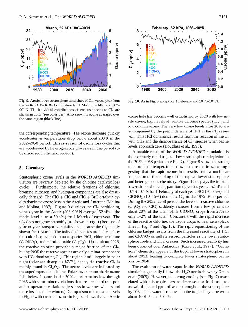
Fig. 9. Arctic lower stratosphere sand chart of Cly versus year fromthe WORLD AVOIDEDsimulation for 1 March, 52 hPa, and 80◦–90◦ N. The individual contributions of various species to Cly areshown in color (see color bar). Also shown is ozone averaged overthe same region (black line).

the corresponding temperature. The ozone decrease quicklyaccelerates as temperatures drop below about 200 K in the2052–2058 period. This is a result of ozone loss cycles thatare accelerated by heterogeneous processes in this period (tobe discussed in the next section).

5 Chemistry

Stratospheric ozone levels in theWORLD AVOIDEDsim-ulation are severely depleted by the chlorine catalytic losscycles. Furthermore, the relative fractions of chlorine,bromine, nitrogen, and hydrogen compounds are also drasti-cally changed. The ClO+ ClO and ClO+ BrO catalytic cy-cles dominate ozone loss in the Arctic and Antarctic (Molinaand Molina, 1987). Figure9 displays the Cly partitioningversus year in the Arctic (80◦–90◦ N average, 52 hPa – themodel level nearest 50 hPa) for 1 March of each year. TheCly does not grow smoothly (as shown in Fig.1) because ofyear-to-year transport variability and because the Cly is onlyshown for 1 March. The individual species are indicated bythe color bar, with dominant species HCl, chlorine nitrate(ClONO2), and chlorine oxide (Cl2O2). Up to about 2025,the reactive chlorine provides a major fraction of the Cly,but by 2035 the reactive species are only a minor componentwith HCl dominating Cly. This region is still largely in polarnight (solar zenith angle>87.7◦), hence, the reactive Cly ismainly found in Cl2O2. The ozone levels are indicated bythe superimposed black line. Polar lower stratospheric ozonefalls below 1 ppmv in the 2020s and remains low through2065 with some minor variations that are a result of transportand temperature variations (less loss in warmer winters andmore loss in colder winters). Comparison of the ozone levelsin Fig. 9 with the total ozone in Fig.4a shows that an Arctic

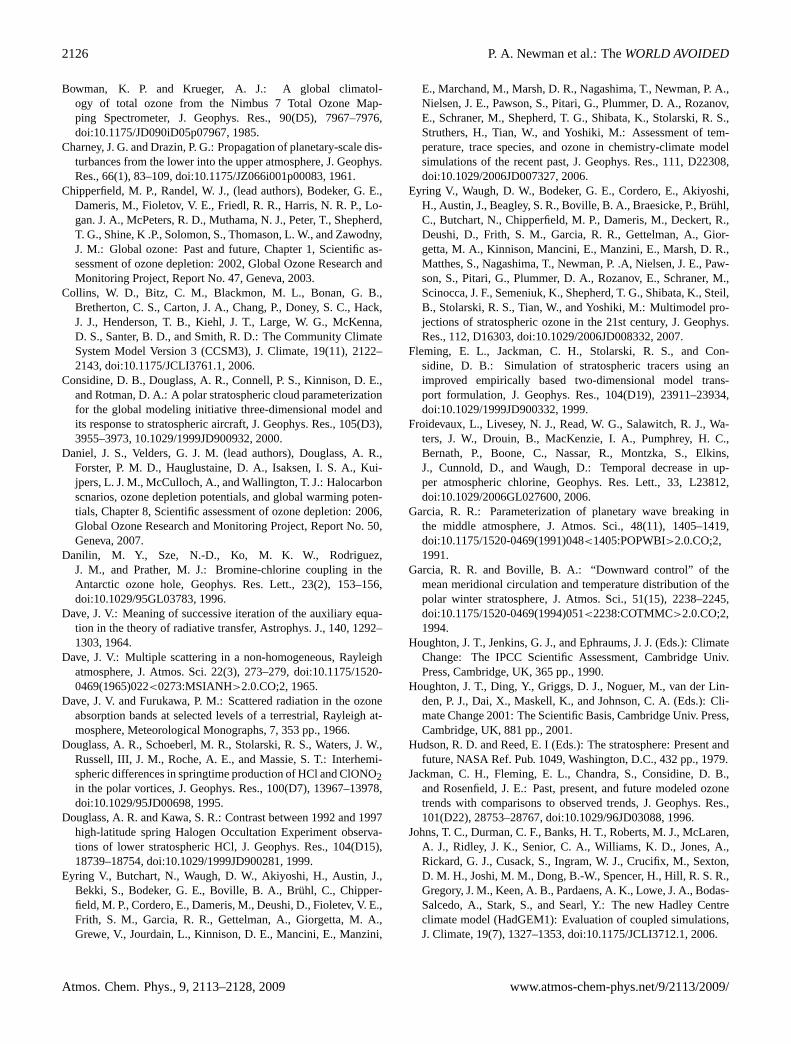
Fig. 10. As in Fig.9 except for 1 February and 10◦ S–10◦ N.

ozone hole has become well established by 2020 with low in-situ ozone, high levels of reactive chlorine species (Clx), andlow column ozone. The very low ozone levels after 2030 areaccompanied by the preponderance of HCl in the Cly reser-voir. This HCl dominance results from the reaction of the Clwith CH4 and the disappearance of Clx species when ozonelevels approach zero (Douglass et al., 1995).

A notable result of theWORLD AVOIDEDsimulation isthe extremely rapid tropical lower stratospheric depletion inthe 2052–2058 period (see Fig.7). Figure8 shows the strongrelationship of temperature to lower stratospheric ozone, sug-gesting that the rapid ozone loss results from a nonlinearinteraction of the cooling of the tropical lower stratosphereand heterogeneous chemistry. Figure10displays the tropicallower stratospheric Cly partitioning versus year at 52 hPa and10◦ S–10◦ N for 1 February of each year. HCl (80–85%) andClONO2 (10–15%) dominate Cly in the 1975–2050 period.During the 2052–2058 period, the levels of reactive chlorine(Cl2O2 and ClO) suddenly increase from a few percent toabout 20% of the total, while ClONO2 drops from 20% toonly 1–2% of the total. Concurrent with the rapid increaseof the reactive chlorine, the ozone drops to near zero (blacklines in Fig.7 and Fig.10). The rapid repartitioning of thechlorine budget results from the increased reactivity of HCland ClONO2 on sulfate aerosol particles as the lower strato-sphere cools and Cly increases. Such increased reactivity hasbeen observed over Antarctica (Kawa et al., 1997). “Ozonehole” chemistry appears in the tropical lower stratosphere inabout 2052, leading to complete lower stratospheric ozoneloss by 2058.

The evolution of water vapor in theWORLD AVOIDEDsimulation generally follows the H2O trends shown byOmanet al.(2009). However, the strong cooling (see Fig.7) asso-ciated with this tropical ozone decrease also leads to a re-moval of about 1 ppm of water throughout the stratosphereby 2060. This water is removed in the tropical layer betweenabout 100 hPa and 50 hPa.



Fig. 11. Annually-averaged temperature difference (K) betweentheWORLD AVOIDEDand thereference futuresimulations for the2055–2065 period. Contour increments are 2 K, while color in-crements are 1 K. The thick black (red) line shows theWORLDAVOIDED (reference future) tropopause. The white lines showstreamlines for the residual circulation differences between theWORLD AVOIDEDand thereference futuresimulations over theperiod. Thicker streamlines indicate increased flow strength.

6 Dynamics and transport

The large ozone depletions in theWORLD AVOIDEDsim-ulation lead to remarkable changes in dynamics and trans-port, including large temperature decreases by the middle ofthe 21st century. Figure11 displays the temperature changebetween theWORLD AVOIDEDandreference futuresimu-lations during the 2055–2065 decade. Cooling is observedeverywhere in this simulation except in the troposphere andat 36 km over Antarctica. The cooling at 1 hPa exceeds 20 K.Shortwave heating at 1 hPa is directly proportional to theozone concentration. As ozone decreases the shortwave heat-ing decreases and the upper stratospheric temperature de-creases.

The warming at 36 km over Antarctica in Fig.11 resultsfrom the dynamical heating caused by the increased down-welling. The white stream lines in the plot show the dif-ference between the residual circulations in theWORLDAVOIDEDandreference futuresimulations. A lifting leads toadditional cooling, while sinking motion causes a dynamicalwarming. The thick black and red lines show the positions ofthe tropopause in both theWORLD AVOIDEDandreferencefuture, respectively. This tropopause is defined with respectto a change in Brunt-Vaisalla frequency. As is clear from theplot, the tropopause increases in altitude at all latitudes as aresult of the stratospheric cooling.

The WORLD AVOIDEDcooling in the tropical lowerstratosphere results from the combined effects of an increaseof the vertical lifting (note the residual circulation stream-lines in Fig. 11) and decreased shortwave heating in the

Fig. 12. Average January zonal-mean zonal wind differences(m s−1) between theWORLD AVOIDEDand thereference futuresimulations for the 2055–2065 period. Contour increments are10 m s−1, while color increments are 5 m s−1. The thick black (red)line shows theWORLD AVOIDED(reference future) tropopause.The white lines show average January zonal-mean wind in theWORLD AVOIDEDsimulation over the period.

tropical lower stratosphere. The shortwave heating remainsroughly constant up to 2045 because of the balancing effectof the UV penetration and ozone changes. As ozone de-creases in the upper stratosphere greater UV flux penetratesto 50 hPa, but as 50-hPa ozone decreases the UV flux absorp-tion decreases, resulting in only very small changes to theshortwave heating. As the increasing tropical lower strato-sphere lifting continues to cool the lower stratosphere, tropi-cal lower stratospheric temperatures cool below the thresholdfor forming stratospheric clouds and heterogeneous chemicalprocesses lead to more ozone loss. The larger ozone lossesthen lead to less shortwave heating which further cools thelower stratosphere, producing a positive feedback that ac-celerates the ozone loss. This positive feedback leads tothe complete collapse of lower stratospheric ozone between2052 and 2058 (Fig.7). This same ozone collapse is alsosimulated in the coupled 2-D modelWORLD AVOIDED.

Changes of ozone and temperature result in zonal-meanzonal wind changes. Figure12 displays the change duringJanuary between thereference futureandWORLD AVOIDEDsimulations averaged over the 2055–2065 period (with themean JanuaryWORLD AVOIDEDzonal winds superimposedas the white lines). In the Southern Hemisphere (SH) themid-summer easterlies in thereference futuresimulation arereplaced with westerlies extending to 1 hPa in theWORLDAVOIDED simulation. The colder SH polar stratosphereleads to a large increase in the tropopause altitude. At 10 hPaand 65◦ S the change is approximately 45 m s−1, while theWORLD AVOIDEDmean winds are slightly higher than40 m s−1. The complete reversal of the usual summer east-erlies indicates that the SH stratosphere has slipped into a



permanent winter across the seasons by 2065. The North-ern Hemisphere (NH) winter polar vortex is slightly weakerin mid-winter in theWORLD AVOIDED, but this differenceis not statistically significant. In contrast to the SH, the NHdoes switch to a summer or easterly circulation in the springbecause the NH tropospheric wave forcing of the strato-sphere is very large in the spring. However, the NH summerstratosphere is significantly colder in the summer becauseof the lack of shortwave heating. In addition to these po-lar vortex results, the upper side of the subtropical jet (30◦ N,70 hPa) is about 5 m s−1 stronger in January.

The large ozone losses also induce changes in the transportof trace species in the stratosphere. Figure13 shows the dif-ference in mean age-of-air between theWORLD AVOIDEDand reference futuresimulations during the 2055–2065 pe-riod. The mean age is calculated in the model by advectinga tracer that increases linearly with time at the surface, andthen computing the time difference at various points of theatmosphere with this age tracer at the tropical tropopause(100 hPa, 20◦ S–20◦ N). Oman et al.(2009) have recentlyshown that there is a near linear decrease of mean age overthe late 20th and 21st centuries in thereference pastandref-erence futuresimulations. In theWORLD AVOIDEDsimula-tion, the large ozone depletion leads to additional decreasesof the mean age-of-air by more than one year in the extrat-ropical stratosphere. Much of this age decrease arises fromthe increase of the vertical lifting. The residual circulationis shown in Figs.11 and13 as the transparent white arrowedlines. Vertical lifting in the tropics (50 hPa, 10◦ S–10◦ N) haschanged from 15 m d−1 in the reference future to 25 m d−1

in theWORLD AVOIDEDsimulation (a 65% increase in up-welling). In addition, there is decreased rising motion above50 hPa (point A in Fig.13). This fresh young air from thetroposphere then spills poleward decreasing the mean age inthe extratropics (point B).

Circulation changes are also apparent in the middle-to-upper stratosphere. The downward circulation (point C inFig. 13) is caused by the changes in the mean zonal winds.As noted byStolarski et al.(2006), the ozone losses causedby the Antarctic ozone hole help the polar vortex persist intothe summer period. The presence of westerly winds in thelate spring and summer allows planetary waves to propa-gate vertically and deposit easterly momentum in the upperstratosphere, inducing a poleward and downward circulationthat would not normally be present. This increased polewardand downward circulation is exacerbated in theWORLDAVOIDED simulation by the additional ozone losses. Theopposite situation is found in the NH (point D). The plan-etary wave deposition of easterly momentum is reduced inthe upper stratosphere, reducing the poleward and downwardcirculation. The small horizontal and vertical gradients ofmean age-of-air in the middle-to-upper stratosphere lead toonly small changes of age in these regions.

Fig. 13.As in Fig.11except for mean age-of-air differences in unitsof years. Contour increments are 0.2 years, while color incrementsare 0.1 years. Letters indicate points of interest in the text.

7 UV changes

As a result of the large ozone depletions, the surface UVreaches extreme levels. To illustrate these changes we havecalculated the surface UV flux in the northern midlatitudesat the height of summer (2 July at local noon) for theWORLD AVOIDEDsimulation. UV calculations were donefor a cloud-free atmosphere using Atmospheric Laboratoryfor Applications and Science 3 (ATLAS-3) extraterrestrial(ET) solar flux and the Total Ozone Mapping Spectrometerradiative transfer (RT) code (TOMRAD). In the TOMRADcode, the atmosphere is assumed to be plane-stratified, withRayleigh scattering (Bates, 1984), WORLD AVOIDEDozoneand temperature profiles, and prescribed surface albedo. Thesolution method is based on the successive iteration of theauxiliary equation of the RT (Dave, 1964, 1965; Dave andFurukawa, 1966). The calculations of atmospheric transmis-sion were done at the original sampling wavelengths of theozone cross-sections measured byBass and Paur(1985) andPaur et al.(1985), with steps≈0.05 nm. The transmittancevalues were linearly interpolated to the vacuum wavelengthsof the high resolution ET solar flux data (ATLAS-3 Solar Ul-traviolet Spectral Irradiance Monitor ET) and multiplied bythe ET spectrum. The TOMRAD RT model compared wellwith spectral irradiance measurements and the output fromother RT models run during the International Photolysis Fre-quency Measurement and Model Intercomparison campaign(Bais et al., 2003).

Figure14displays the flux as a function of wavelength for1980, 2040, and 2065. The vast majority of the UV increaseoccurs at wavelengths less than 310 nm. Figure15shows theratio of the 2000, 2020, 2040, and 2065 UV flux to the 1980UV flux. At wavelengths below 308 nm the UV flux has morethan doubled by 2065, and the flux has increased by a fac-tor of 1000 for wavelengths less than 291 nm. At 280 nm in



Fig. 14. UV flux (W m−2 nm−1) is shown for theWORLDAVOIDEDsimulation in 1980, 2040, and 2065 (thick black lines).The UV flux is calculated using the July 30◦–50◦ N zonal-meanozone and temperature profiles, and assuming a time of local noonon 2 July. The thick grey line shows the erythemal (sunburn) actionspectrum (right hand axis). The thin darker grey line shows UV fluxat the top of the atmosphere.

Fig. 15. The ratio of the UV flux (from Fig.14) for 2000, 2020,2040, and 2065 to its value in 1980. The horizontal grey lines in-dicate a doubling and a factor of 1000 from the 1980 conditions.The vertical lines indicate where the 2065 curve crosses these twolevels.

2065, theWORLD AVOIDEDUV flux is 109 times strongerthan the 1980 flux level (off scale).

We have calculated the UV index for midlatitude NHconditions in mid-summer (a relatively densely populatedzone on the globe). Figure16 shows this UV index for theWORLD AVOIDED, reference future, andfixed chlorinesim-ulations. For mid-summer clear-sky conditions, the UV in-dex is normally very high at local noon; with a typical timeto produce a perceptible sun burn (type II skin) of about 10–

Fig. 16. UV index versus year for theWORLD AVOIDED(black),reference future(red), andfixed chlorine(green) simulations. Aswith Fig. 14, the UV index is calculated using the July 30◦–50◦ Nzonal-mean ozone, and assuming a time of local noon on 2 July. Thestandard UV index “risk” scale is also superimposed on the bottomleft. The horizontal grey line shows the 1975–1985 average of theUV index from thefixed chlorinesimulation.

20 min. The mid-summer period has the highest UV indexover the course of the year. The differences between theref-erence futureandfixed chlorinesimulations show increaseson the order of 5–10% by 2000. TheWORLD AVOIDEDsimulation has the UV index nearing 15 by 2040 and exceed-ing a value of 30 by 2065. This extreme value of the UVindex would reduce the perceptible sunburn time from ap-proximately 15 min to about 5 min. The UV index valuesalso increase by 2065 to large values at both the eqator (33in early March) and SH midlatitudes (35 at 40 S for mid-January).

These extreme UV increases would also lead to large in-creases of skin cancer (Slaper et al., 1996). In the same man-ner as estimating the UV index, we apply a DNA damageaction spectrum to our UV spectrum calculations (Setlow,1974). The DNA damaging UV for the NH midlatitudes in-creases by approximately 550% between 1980 and 2065.

8 Summary

In this study we have simulated the effects on the stratosphereof a steady growth of ozone-depleting substances and com-pared those results to the normal expectations of the evolu-tion of the stratosphere in the 21st century. As was suggestedby the originalMolina and Rowland(1974) study on CFCsin the stratosphere, large concentrations of ODSs in the at-mosphere would have virtually destroyed the majority of theozone layer by 2065 (global annual average losses>60%).



Very large ozone losses are computed at all latitudes inthe stratosphere of theWORLD AVOIDEDsimulation. Thelargest losses in both percentage and Dobson Units are in thepolar latitudes. However, surprisingly large losses also oc-cur in tropical latitudes as a result of heterogeneous chemi-cal processes that occur in the 2052–2058 period. This “polarchemistry” in the tropics begins to appear in the lower strato-sphere as a consequence of cooling resulting from increasedvertical lifting.

Most of the ozone depletion occurs in the lower strato-sphere (12–24 km) and the upper stratosphere (≈42 km).Losses inside the polar vortex in both hemispheres exceed90% by 2065. At 20 km, annual average tropical levels arereduced by 80%. Ozone losses in the upper stratosphere ex-ceed 60%. Middle stratosphere ozone losses are smaller, butstill greater than 40%.

As in current observations, the largest losses occur in thespring polar regions. Over Antarctica, the ozone hole devel-ops quickly in the 1980–2000 period, with somewhat slowertrends after 2000 as a result of the complete ozone destruc-tion in the lower stratosphere. October column values dropfrom 400 DU (somewhat higher than historic observations)to values of about 60 DU by 2065 (85% loss). By 2040,the SH stratosphere ozone values are so low that interan-nual variability of the dynamics and transport has virtuallyno impact on total ozone, such that the total ozone internan-nual variability is near zero. In the Arctic, ozone declines aremore linear with April total ozone dropping from values near500 DU to about 100 DU in 2065 (an 80% decline). The an-nual ozone mixing ratios in the Antarctica and Arctic lowerstratosphere (15–20 km) are nearly zero.

The severe ozone depletions lead to interesting dynamicalchanges. The SH westerly circulation persists virtually year-round by 2035, although temperatures still exceed 195 K inthe late spring. This westerly circulation allows the verti-cal propagation of planetary scale waves (westerly winds arenecessary for the vertical propagation of large scale Rossbywaves) (Charney and Drazin, 1961). The deposition of east-erly momentum from these waves then drives a polewardand downward circulation. In the NH stratosphere, the mid-winter dynamical changes are surprisingly small. The strato-spheric polar night jet remains virtually the same. By 2055,the vertical circulation in the tropics (50 hPa, 10◦ S–10◦ N)has increased by about 65%. This increased upwelling coolsthe lower stratosphere leading to the onset of heterogeneouschemistry and the collapse of ozone in the lower stratospherein the 2052–2058 period.

Our WORLD AVOIDEDsimulation is limited in a few re-spects. First, the simulation was performed with specifiedSSTs that were simulated by the NCAR CCM3 using theIPCC A1b scenario. Hence, our tropospheric temperaturesdo not correctly respond to the increased CFC radiative forc-ing or stratospheric changes. Second, the model does notinclude tropospheric chemistry (i.e., the tropospheric ozonevalues are relaxed to the climatology ofLogan, 1999) and

thus tropospheric ozone changes are not discussed in thisstudy. Because tropospheric ozone is not explicitly mod-eled, the radiative forcing on the troposphere of troposphericozone is not correct. Since the tropospheric climage changesare not correctly simulated, the complete tropospheric ef-fect on the stratosphere is not correctly simulated (e.g., thechanges in vertical wave propagation from the troposphereto the stratosphere). Third, since the tropospheric chemistryis not modeled, the simulated surface UV changes are lim-ited to those only caused by the stratosphere. Fourth, theGEOSCCM is forced by scenario estimates of surface mix-ing ratios of both greenhouse gases and CFCs. The increasedstratospheric circulation will shorten the lifetimes of CFCs.The increased UV that penetrates to the troposphere mightincrease the hydroxyl radical, increasing the oxidizing capac-ity of the troposphere and thereby shortening the lifetimes ofgases such as CH4 and HCFCs. Hence, feedback of the UVand circulation would affect the evolution of both climate andozone depleting gases.

Acknowledgements.This work was supported under the NASAAtmospheric Chemistry Modeling and Analysis Program andthe Modeling, Analysis, and Prediction Program. GEOS CCMsimulations were performed on NASA’s Columbia platform usingresources provided by NASA’s High-End Computing initiative. Weare also grateful for the helpful comments provided by David Faheyand several reviewers.

Edited by: M. Dameris

References

Anderson, J., Russell, III, J. M., Solomon, S., and Deaver,L. E.: Halogen Occultation Experiment confirmation of strato-spheric chlorine decreases in accordance with the Mon-treal Protocol, J. Geophys. Res., 105(D4), 4483–4490,doi:10.1029/1999JD901075, 2000.

Bais, A. F., Madronich, S., Crawford, J., Hall, S. R., Mayer, B.,van Weele, M., Lenoble, J., Calvert, J. G., Cantrell, C. A., Shet-ter, R. E., Hofzumahaus, A., Koepke, P., Monks, P. S., Frost, G.,McKenzie, R., Krotkov, N., Kylling, A., Swartz, W. H., Lloyd,S., Pfister, G., Martin, T. J., Roeth, E.-P., Griffioen, E., Ruggaber,A., Krol, M., Kraus, A., Edwards, G. D., Mueller, M., Lefer,B. L., Johnston, P., Schwander, H., Flittner, D., Gardiner, B. G.,Barrick, J., and Schmitt, R.: International Photolysis FrequencyMeasurement and Model Intercomparison (IPMMI): Spectral ac-tinic solar flux measurements and modeling, J. Geophys. Res.,108(D16), 8543, doi:10.1029/2002JD002891, 2003.

Bass, A. M. and Paur, R. J.: The ultraviolet cross-sections of ozone:I. The measurements, Atmospheric Ozone: Proceedings of theQuadrennial Ozone Symposium held in Halkidiki, Greece, 3–7September 1984, edited by: Zerefos, C. S. and Ghazi, A., Reidel,Dordrecht, Holland, 606–610, 1985.

Bates, D. R.: Rayleigh scattering by air, Planet. Space Sci., 32(6),785–790, doi:10.1016/0032-0633(84)90102-8, 1984.

Bosilovich, M. G., Schubert, S. D., and Walker, G. K.: Globalchanges of the water cycle intensity, J. Climate, 18(10), 1591–1608, doi:10.1175/JCLI3357.1, 2005.



Bowman, K. P. and Krueger, A. J.: A global climatol-ogy of total ozone from the Nimbus 7 Total Ozone Map-ping Spectrometer, J. Geophys. Res., 90(D5), 7967–7976,doi:10.1175/JD090iD05p07967, 1985.

Charney, J. G. and Drazin, P. G.: Propagation of planetary-scale dis-turbances from the lower into the upper atmosphere, J. Geophys.Res., 66(1), 83–109, doi:10.1175/JZ066i001p00083, 1961.

Chipperfield, M. P., Randel, W. J., (lead authors), Bodeker, G. E.,Dameris, M., Fioletov, V. E., Friedl, R. R., Harris, N. R. P., Lo-gan. J. A., McPeters, R. D., Muthama, N. J., Peter, T., Shepherd,T. G., Shine, K .P., Solomon, S., Thomason, L. W., and Zawodny,J. M.: Global ozone: Past and future, Chapter 1, Scientific as-sessment of ozone depletion: 2002, Global Ozone Research andMonitoring Project, Report No. 47, Geneva, 2003.

Collins, W. D., Bitz, C. M., Blackmon, M. L., Bonan, G. B.,Bretherton, C. S., Carton, J. A., Chang, P., Doney, S. C., Hack,J. J., Henderson, T. B., Kiehl, J. T., Large, W. G., McKenna,D. S., Santer, B. D., and Smith, R. D.: The Community ClimateSystem Model Version 3 (CCSM3), J. Climate, 19(11), 2122–2143, doi:10.1175/JCLI3761.1, 2006.

Considine, D. B., Douglass, A. R., Connell, P. S., Kinnison, D. E.,and Rotman, D. A.: A polar stratospheric cloud parameterizationfor the global modeling initiative three-dimensional model andits response to stratospheric aircraft, J. Geophys. Res., 105(D3),3955–3973, 10.1029/1999JD900932, 2000.

Daniel, J. S., Velders, G. J. M. (lead authors), Douglass, A. R.,Forster, P. M. D., Hauglustaine, D. A., Isaksen, I. S. A., Kui-jpers, L. J. M., McCulloch, A., and Wallington, T. J.: Halocarbonscnarios, ozone depletion potentials, and global warming poten-tials, Chapter 8, Scientific assessment of ozone depletion: 2006,Global Ozone Research and Monitoring Project, Report No. 50,Geneva, 2007.

Danilin, M. Y., Sze, N.-D., Ko, M. K. W., Rodriguez,J. M., and Prather, M. J.: Bromine-chlorine coupling in theAntarctic ozone hole, Geophys. Res. Lett., 23(2), 153–156,doi:10.1029/95GL03783, 1996.

Dave, J. V.: Meaning of successive iteration of the auxiliary equa-tion in the theory of radiative transfer, Astrophys. J., 140, 1292–1303, 1964.

Dave, J. V.: Multiple scattering in a non-homogeneous, Rayleighatmosphere, J. Atmos. Sci. 22(3), 273–279, doi:10.1175/1520-0469(1965)022<0273:MSIANH>2.0.CO;2, 1965.

Dave, J. V. and Furukawa, P. M.: Scattered radiation in the ozoneabsorption bands at selected levels of a terrestrial, Rayleigh at-mosphere, Meteorological Monographs, 7, 353 pp., 1966.

Douglass, A. R., Schoeberl, M. R., Stolarski, R. S., Waters, J. W.,Russell, III, J. M., Roche, A. E., and Massie, S. T.: Interhemi-spheric differences in springtime production of HCl and ClONO2in the polar vortices, J. Geophys. Res., 100(D7), 13967–13978,doi:10.1029/95JD00698, 1995.

Douglass, A. R. and Kawa, S. R.: Contrast between 1992 and 1997high-latitude spring Halogen Occultation Experiment observa-tions of lower stratospheric HCl, J. Geophys. Res., 104(D15),18739–18754, doi:10.1029/1999JD900281, 1999.

Eyring V., Butchart, N., Waugh, D. W., Akiyoshi, H., Austin, J.,Bekki, S., Bodeker, G. E., Boville, B. A., Bruhl, C., Chipper-field, M. P., Cordero, E., Dameris, M., Deushi, D., Fioletev, V. E.,Frith, S. M., Garcia, R. R., Gettelman, A., Giorgetta, M. A.,Grewe, V., Jourdain, L., Kinnison, D. E., Mancini, E., Manzini,

E., Marchand, M., Marsh, D. R., Nagashima, T., Newman, P. A.,Nielsen, J. E., Pawson, S., Pitari, G., Plummer, D. A., Rozanov,E., Schraner, M., Shepherd, T. G., Shibata, K., Stolarski, R. S.,Struthers, H., Tian, W., and Yoshiki, M.: Assessment of tem-perature, trace species, and ozone in chemistry-climate modelsimulations of the recent past, J. Geophys. Res., 111, D22308,doi:10.1029/2006JD007327, 2006.

Eyring V., Waugh, D. W., Bodeker, G. E., Cordero, E., Akiyoshi,H., Austin, J., Beagley, S. R., Boville, B. A., Braesicke, P., Bruhl,C., Butchart, N., Chipperfield, M. P., Dameris, M., Deckert, R.,Deushi, D., Frith, S. M., Garcia, R. R., Gettelman, A., Gior-getta, M. A., Kinnison, Mancini, E., Manzini, E., Marsh, D. R.,Matthes, S., Nagashima, T., Newman, P. .A, Nielsen, J. E., Paw-son, S., Pitari, G., Plummer, D. A., Rozanov, E., Schraner, M.,Scinocca, J. F., Semeniuk, K., Shepherd, T. G., Shibata, K., Steil,B., Stolarski, R. S., Tian, W., and Yoshiki, M.: Multimodel pro-jections of stratospheric ozone in the 21st century, J. Geophys.Res., 112, D16303, doi:10.1029/2006JD008332, 2007.

Fleming, E. L., Jackman, C. H., Stolarski, R. S., and Con-sidine, D. B.: Simulation of stratospheric tracers using animproved empirically based two-dimensional model trans-port formulation, J. Geophys. Res., 104(D19), 23911–23934,doi:10.1029/1999JD900332, 1999.

Froidevaux, L., Livesey, N. J., Read, W. G., Salawitch, R. J., Wa-ters, J. W., Drouin, B., MacKenzie, I. A., Pumphrey, H. C.,Bernath, P., Boone, C., Nassar, R., Montzka, S., Elkins,J., Cunnold, D., and Waugh, D.: Temporal decrease in up-per atmospheric chlorine, Geophys. Res. Lett., 33, L23812,doi:10.1029/2006GL027600, 2006.

Garcia, R. R.: Parameterization of planetary wave breaking inthe middle atmosphere, J. Atmos. Sci., 48(11), 1405–1419,doi:10.1175/1520-0469(1991)048<1405:POPWBI>2.0.CO;2,1991.

Garcia, R. R. and Boville, B. A.: “Downward control” of themean meridional circulation and temperature distribution of thepolar winter stratosphere, J. Atmos. Sci., 51(15), 2238–2245,doi:10.1175/1520-0469(1994)051<2238:COTMMC>2.0.CO;2,1994.

Houghton, J. T., Jenkins, G. J., and Ephraums, J. J. (Eds.): ClimateChange: The IPCC Scientific Assessment, Cambridge Univ.Press, Cambridge, UK, 365 pp., 1990.

Houghton, J. T., Ding, Y., Griggs, D. J., Noguer, M., van der Lin-den, P. J., Dai, X., Maskell, K., and Johnson, C. A. (Eds.): Cli-mate Change 2001: The Scientific Basis, Cambridge Univ. Press,Cambridge, UK, 881 pp., 2001.

Hudson, R. D. and Reed, E. I (Eds.): The stratosphere: Present andfuture, NASA Ref. Pub. 1049, Washington, D.C., 432 pp., 1979.

Jackman, C. H., Fleming, E. L., Chandra, S., Considine, D. B.,and Rosenfield, J. E.: Past, present, and future modeled ozonetrends with comparisons to observed trends, J. Geophys. Res.,101(D22), 28753–28767, doi:10.1029/96JD03088, 1996.

Johns, T. C., Durman, C. F., Banks, H. T., Roberts, M. J., McLaren,A. J., Ridley, J. K., Senior, C. A., Williams, K. D., Jones, A.,Rickard, G. J., Cusack, S., Ingram, W. J., Crucifix, M., Sexton,D. M. H., Joshi, M. M., Dong, B.-W., Spencer, H., Hill, R. S. R.,Gregory, J. M., Keen, A. B., Pardaens, A. K., Lowe, J. A., Bodas-Salcedo, A., Stark, S., and Searl, Y.: The new Hadley Centreclimate model (HadGEM1): Evaluation of coupled simulations,J. Climate, 19(7), 1327–1353, doi:10.1175/JCLI3712.1, 2006.



Kawa, S. R., Newman, P. A., Lait, L. R., Schoeberl, M. R., Stimpfle,R. M., Kohn, D. W., Webster, C. R., May, R. D., Baumgard-ner, D., Dye, J. E., Wilson, J. C., Chan, K. R., and Loewenstein,M.: Activation of chlorine in sulfate aerosol as inferred fromaircraft observations, J. Geophys. Res., 102(D3), 3921–3933,doi:10.1175/96JD01992, 1997.

Kiehl, J. T., Hack, J. J., Bonan, G. B., Boville, B. A.,Williamson, D. L., and Rasch, P. J.: The National Cen-ter for Atmospheric Research Community Climate Model:CCM3, J. Climate, 11(6), 1131–1149, doi:10.1175/1520-0442(1998)011<1131:TNCFAR>2.0.CO;2, 1998.

Lary, D. J., Waugh, D. W., Douglass, A. R., Stolarski, R. S., New-man, P. A., and Mussa, H.: Variations in stratospheric inor-ganic chlorine between 1991 and 2006, Geophys. Res. Lett., 34,L21811, doi:10.1029/2007GL030053, 2007.

Lin, S.-J.: A “vertically Lagrangian” finite-volume dynamical corefor global models, Mon. Weather Rev., 132(10), 2293–2307,doi:10.1175/1520-0493(2004)132<2293:AVLFDC>2.0.CO;2,2004.

Logan, J. A.: An analysis of ozonesonde data for the troposphere:Recommendations for testing 3-D models and development ofa gridded climatology for tropospheric ozone, J. Geophys. Res.,104(D13), 16115–16150, doi:10.1029/1998JD100096, 1999.

Molina, M. J. and Rowland, F. S.: Stratospheric sink for chloroflu-oromethanes: Chlorine atom catalyzed destruction of ozone, Na-ture, 249, 810–812, doi:10.1038/249810a0, 1974.

Molina, L. T. and Molina, M. J.: Production of chlorine oxide(Cl2O2) from the self-reaction of the chlorine oxide (ClO) radi-cal, J. Phys. Chem., 91(2), 433–436, doi:10.1021/j100286a035,1987.

Montzka, S. A., Butler, J. H., Myers, R. C., Thompson, T. M.,Swanson, T. H., Clarke, A. D., Lock, L. T., and Elkins, J. W.:Decline in the tropospheric abundance of halogen from halocar-bons: Implications for stratospheric ozone depletion, Science,272(5266), 1318–1322, doi:10.1126/science.272.5266.1318,1996.

Montzka, S. A., Fraser, P. J., (lead authors), Butler, J. H., Connell,P. S., Cunnold, D. M., Daniel, J. S., Derwent, R. G., Lal, S., Mc-Culloch, A., Oram, D. E., Reeves, C. E., Sanhueza, E., Steele,L. P., Velders, G. J., M., Weiss, R. F., and Zander, R. J.: Con-trolled substances and other source gases, Chapter 1, Scientificassessment of ozone depletion: 2002, Global Ozone Researchand Monitoring Project, Report No. 47, Geneva, 2003.

Morgenstern, O., Braesicke, P., Hurwitz, M. M., O’Connor, F. M.,Bushell, A. C., Johnson, C. E., and Pyle, J. A.: The worldavoided by the Montreal Protocol, Geophys. Res. Lett., 35,L16811, doi:10.1029/2008GL034590, 2008.

Newman, P. A., Daniel, J. S., Waugh, D. W., and Nash, E. R.:A new formulation of equivalent effective stratospheric chlorine(EESC), Atmos. Chem. Phys., 7, 4537–4552, 2007,http://www.atmos-chem-phys.net/7/4537/2007/.

Oman, L., Waugh, D. W., Pawson, S., Stolarski, R. S., and Newman,P. A.: On the influence of anthropogenic forcings on changesin the stratospheric mean age, J. Geophys. Res., 114, D03105,doi:10.1029/2008JD010378, 2009.

Paur, R. J. and Bass, A. M.: The ultraviolet cross-sections ofozone: II. Results and temperature dependence, in AtmosphericOzone: Proceedings of the Quadrennial Ozone Symposium heldin Halkidiki, Greece, 3–7 September 1984, edited by: Zerefos,

C. S. and Ghazi, A., Reidel, Dordrecht, Holland, 606–610, 1985.Pawson S., Stolarski, R. S., Douglass, A. R., Newman, P. A.,

Nielsen, J. E., Frith, S. M., and Gupta, M. L.: Goddard Earth Ob-serving System chemistry-climate model simulations of strato-spheric ozone-temperature coupling between 1950 and 2005, J.Geophys. Res., 113, D12103, doi:10.1029/2007JD009511, 2008.

Plumb, R. A. and Mahlman, J. D.: The zonally averaged trans-port characteristics of the GFDL general circulation/transportmodel, J. Atmos. Sci., 44(2), 298–327, doi:10.1175/1520-0469(1987)044<0298:TZATCO>2.0.CO;2, 1987.

Prather, M., Midgley, P., Rowland, F. S., and Stolarski, R.:The ozone layer: The road not taken, Nature, 381, 551–554,doi:10.1038/381551a0, 1996.

Ramanathan, V., Cicerone, R. J., Singh, H. B., and Kiehl,J. T.: Trace gas trends and their potential role in cli-mate change, J. Geophys. Res., 90(D3), 5547–5566,doi:10.1029/JD090iD03p05547, 1985.

Rayner, N. A., Parker, D. E., Horton, E. B., Folland, C. K., Alexan-der, L. V., Rowell, D. P., Kent, E. C., and Kaplan, A.: Globalanalyses of sea surface temperature, sea ice, and night marine airtemperature since the late nineteenth century, J. Geophys. Res.,108(D14), 4407, doi:10.1029.2002JD002670, 2003.

Rosenfield, J. E., Douglass, A. R., and Considine, D. B.: The im-pact of increasing carbon dioxide on ozone recovery, J. Geophys.Res., 107(D6), 4049, doi:10.1029/2001JD000824, 2002.

Sander, S. P., Friedl, R. R., Ravishankara, A. R., Golden, D. M.,Kolb, C. E., Kurylo, M. J., Huie, R. E., Orkin, V. L., Molina,M. J., Moortgat, G. K., and Finlayson-Pitts, B. J.: Chemicalkinetics and photochemical data for use in atmospheric studies,Evaluation 14, JPL Pub. 02-25, Pasadena, 2003.

Sarma, K. M. and Bankobeza, G. M. (Eds.): The Montreal proto-col on substances that deplete the ozone layer, United NationsEnvironment Programme, Nairobi, Kenya, 2000.

Setlow, R. B.: The wavelengths in sunlight effective in producingskin cancer: A theoretical analysis, Proc. Natl. Acad. Sci. USA,71(9), 3363–3366, 1974.

Slaper, H., Velders, G. J. M., Daniel, J. S., de Gruijl, F. R., andvan der Leun, J. C.: Estimates of ozone depletion and skin can-cer incidence to examine the Vienna Convention achievements,Nature, 384, 256–258, doi:10.1038/384256a0, 1996.

Solomon S., Portmann, R. W., Sasaki, T., Hofmann, D. J.,and Thompson, D. W. J.: Four decades of ozonesonde mea-surements over Antarctica, J. Geophys. Res., 110, D21311,doi:10.1029/2005JD005917, 2005.

Stolarski, R. S., Douglass, A. R., Gupta, M., Newman, P. A., Paw-son, S., Schoeberl, M. R., and Nielsen, J. E.: An ozone in-crease in the Antarctic summer stratosphere: A dynamical re-sponse to the ozone hole, Geophys. Res. Lett., 33, L21805,doi:10.1029/2006GL026820, 2006.

Tripathi, O. P., Godin-Beekmann, S., Lefevre, F., Pazmino, A.,Hauchecorne, A., Chipperfield, M., Feng, W., Millard, G.,Rex, M., Streibel, M., and von der Gathen, P.: Comparisonof polar ozone loss rates simulated by one-dimensional andthree-dimensional models with Match observations in recentAntarctic and Arctic winters, J. Geophys. Res., 112, D12307,doi:10.1029/2006JD008370, 2007.

Velders, G. J. M., Andersen, S. O., Daniel, J. S., Fahey, D. W.,and McFarland, M.: The importance of the Montreal Protocol inprotecting climate, Proc. Natl. Acad. Sci. USA, 104(12), 4814–


http://www.atmos-chem-phys.net/7/4537/2007/


4819, 10.1073/pnas.0610328104, 2007.World Meteorological Organization (WMO): Atmospheric Ozone

1985, Global Ozone Research and Monitoring Project, ReportNo. 16,, Geneva, Switzerland, 1985.

Yudin, V. A., Smyshlyaev, S. P., Geller, M. A., and Dvortsov,V. L.: Transport diagnostics of GCMs and implicationsfor 2D chemistry-transport model of troposphere and strato-sphere, J. Atmos. Sci., 57(5), 673–699, doi:10.1175/1520-0469(2000)057<0673:TDOGAI>2.0.CO;2, 2000.


What would have happened to the ozone layer if ...€¦ · ozone depletion, a failure to regulate...

Documents

Transcript of What would have happened to the ozone layer if ...€¦ · ozone depletion, a failure to regulate...