Harvard-MIT Division of Health Sciences and Technology

HST.725: Music Perception and Cognition

Prof. Peter Cariani

HST 725Music Perception & Cognition

Lecture 2

What we hear:

Basic dimensions of auditory experience

www.cariani.com(Image removed due to copyright considerations.)

What we hear: dimensions of auditory experience

• Hearing: ecological functions (distant warning, communication, prey detection; works in the dark)

• Detection, discrimination, recognition, reliability, scene analysis• Operating range: thresholds, ceilings, & frequency limits

• Independent dimensions of hearing & general properties

– Pitch

– Timbre (sound quality)

– Loudness

– Duration

– Location

– Distance and Size

• Perception of isolated pure tones

• Interactions of sounds: beatings, maskings, fusions

• Masking (tones vs. tones, tones in noise)

• Fusion of sounds & the auditory "scene":

– how many objects/sources/voices/streams?

• Representation of periodicity and spectrum

• Power spectrum and auditory filter metaphors

• Analytical (Helmholtz) vs. Gestalt (Stumpf) perspectives

Hearing: ecological functions

• Distant warning of predators approaching

• Identification of predators

• Localization/tracking of prey

• Con-specific communication

Mating/competition

Cooperation (info. sharing)

Territory

• Navigation in the dark

http://www.pbs.org/wgbh/nova/wolves/

http://www.pbs.org/lifeofbirds/songs/index.html

bat-eared fox

http://www.essex.ac.uk/psychology/hearinglab/index.htm

The auditory scene:

basic dimensions

Temporal organization • Events

• Notes

• Temporal patterns of events

Organization of sounds • Voices, instruments

• Streams

• Objects

• Sources

Attributes of sounds • Loudness (intensity)

• Pitch (dominant periodicity)• Timbre (spectrum)

• Duration

• Location (bearing, range)

Auditory qualities in music perception & cognition

• Pitch Melody, harmony, consonance

• Timbre Instrument voices

• Loudness Dynamics

• Organization Fusions, objects. How many voices?

• Rhythm Temporal organization of events

• Longer pattern Repetition, sequence

• Mnemonics Familiarity, novelty

• Hedonics Pleasant/unpleasant

• Affect Emotional associations, meanings

• Semantics Cognitive associations/expectations

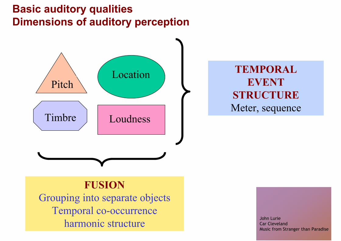
Basic auditory qualities

Dimensions of auditory perception

Pitch Location

LoudnessTimbre

TEMPORALEVENT

STRUCTUREMeter, sequence

FUSION

Grouping into separate objectsTemporal co-occurrence

harmonic structureJohn Lurie

Car Cleveland

Music from Stranger than Paradise

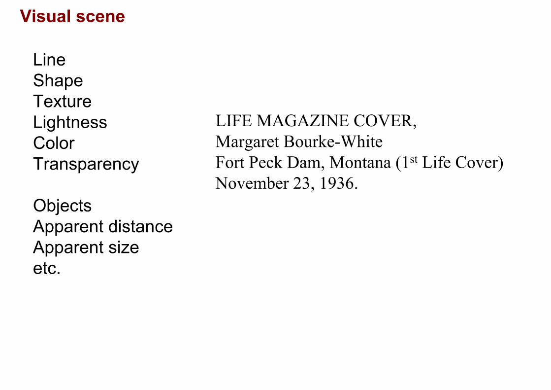
Visual scene

LineShapeTextureLightnessColorTransparency

Objects

Apparent distance

Apparent size

etc.

LIFE MAGAZINE COVER,Margaret Bourke-WhiteFort Peck Dam, Montana (1st Life Cover)November 23, 1936.

Sound level basics

• Sound pressure levels are measured relative to an absolute reference

• (re: 20 micro-Pascals, denoted Sound Pressure Level or SPL).• Since the instantaneous sound pressure fluctuates, the

average amplitude of the pressure waveform is measured using root-mean-square RMS. (Moore, pp. 9-12)

• Rms(x) = sqrt(mean(sum(xt2)))

– Where xt is the amplitude of the waveform at each instant t in the sample

– Because the dynamic range of audible sound is so great, magnitudes are expressed in a logarithmic scale, decibels (dB).

• A decibel of amplitude expresses the ratio of two amplitudes (rms pressures, P1 and P_reference) and is given by the equation:

dB = 20 * log10(P1/P_reference)20 dB = 10 fold change in rms level

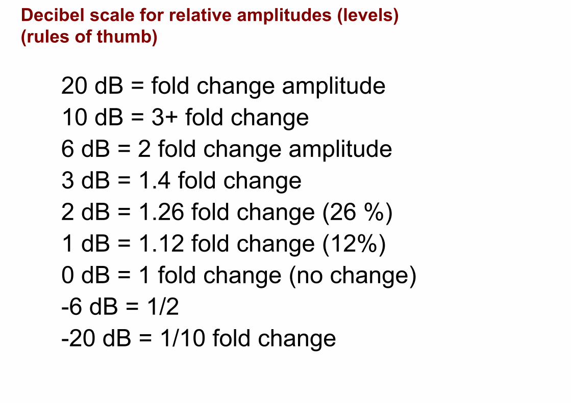
Decibel scale for relative amplitudes (levels)

(rules of thumb)

20 dB = fold change amplitude

10 dB = 3+ fold change

6 dB = 2 fold change amplitude

3 dB = 1.4 fold change

2 dB = 1.26 fold change (26 %)

1 dB = 1.12 fold change (12%)

0 dB = 1 fold change (no change)

-6 dB = 1/2

-20 dB = 1/10 fold change

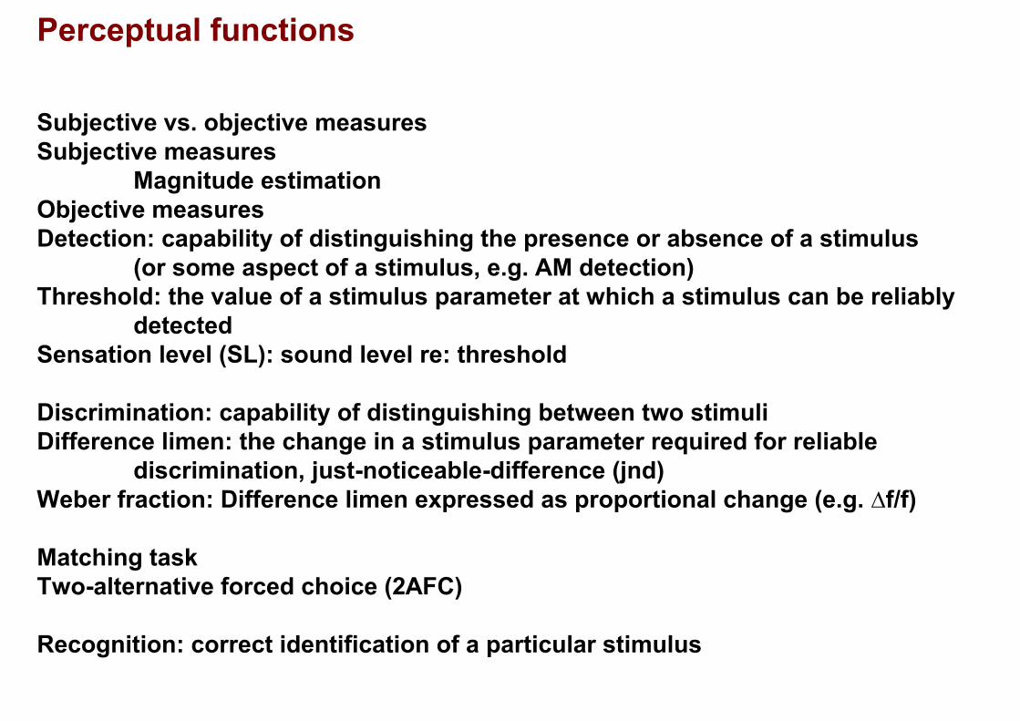
Perceptual functions

Subjective vs. objective measures

Subjective measures

Magnitude estimationObjective measures

Detection: capability of distinguishing the presence or absence of a stimulus (or some aspect of a stimulus, e.g. AM detection)

Threshold: the value of a stimulus parameter at which a stimulus can be reliably

detected

Sensation level (SL): sound level re: threshold

Discrimination: capability of distinguishing between two stimuli

Difference limen: the change in a stimulus parameter required for reliable

discrimination, just-noticeable-difference (jnd)

Weber fraction: Difference limen expressed as proportional change (e.g. ¨f/f)

Matching task

Two-alternative forced choice (2AFC)

Recognition: correct identification of a particular stimulus

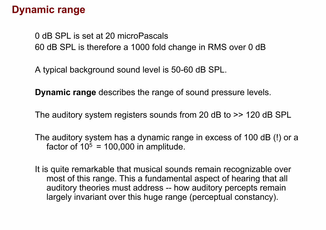
Dynamic range

0 dB SPL is set at 20 microPascals

60 dB SPL is therefore a 1000 fold change in RMS over 0 dB

A typical background sound level is 50-60 dB SPL.

Dynamic range describes the range of sound pressure levels.

The auditory system registers sounds from 20 dB to >> 120 dB SPL

The auditory system has a dynamic range in excess of 100 dB (!) or a factor of 105 = 100,000 in amplitude.

It is quite remarkable that musical sounds remain recognizable over most of this range. This a fundamental aspect of hearing that all auditory theories must address -- how auditory percepts remain largely invariant over this huge range (perceptual constancy).

On origins of music dynamics notation Typical sound levels in music http://www.wikipedia.org/wiki/Pianissimo

In music , the word dynamics refers to

the volume of the sound . The

renaissance composer Giovanni

Gabrieli was one of the first to indicate

dynamics in music notation .The two

basic dynamic indications in music are

• > 130 dB SPLPain piano , meaning "softly" or "quietly",

usually abbreviated as p; and forte ,

meaning "loudly" or "strong", usually

abbreviated as f. More subtle degrees • Loud rock concert 120 dB SPL of loudness or softness are indicated by

mp , standing for mezzo-piano , and• Loud disco 110 dB SPLmeaning "half-quiet"; and mf ,mezzo-

forte , "half loud". Beyond fand p, there • fff 100 dB SPL is ff , standing for "fortissimo", and

meaning "very loudly"; and pp , standing for "pianissimo", and meaning • f 80 dB SPL(forte, strong) "very quietly". To indicate even more

extreme degrees of intensity, more ps

or fs are added as required. fff (fortississimo ) and ppp (pianississimo )

are found in sheet music quite

• p 60 dB SPL(piano, soft)

• ppp 40 dB SPL frequently, but more than three fs or ps

is quite rare. It is sometimes said that

pppp stands for pianissississimo , but

such words are very rarely used either

in speech or writing, even when present

in a score. There is some evidence that

this use of an increasing number of

letters to indicate greater extremes of

• Lower limit

• Theshold of hearing 0 dB SPL volume stems from a convention dating

from the 17th century where pstood for

piano ,pp stood for più piano (literally

"more quietly") and, by extension, ppp • Musical notation ranges from Pierce, Science of Musical Sound, p. 325 indicated pianissimo .Antonio Vivaldi

seems to have written using this

convention, but it was largely replaced

by the above, more familiar, system by

the middle of the 18th century .

Typical sound pressure levels in everyday life

Disco

(Reproduced courtesy of WorkSafe, Department of Consumer and Employment Protection, Western Australia (www.safetyline.wa.gov.au).The graphic being that at the bottom of: http://www.safetyline.wa.gov.au/institute/level2/course18/lecture54/l54_03.asp)

Demonstrations

• Demonstrations using waveform generator

• Relative invariance of pitch & timbre with level

• Loudness matching

• Pure tone frequency limits

• Localization

Loudness

Dimension of perception that changes with

sound intensity (level)

Intensity ~ power;

Level~amplitude

Demonstration using waveform generator

Masking demonstrations

Magnitude estimation

Loudness matching

Sound level meters and frequency weightings

2-45-40-35-30-25-20-15-10-505

224 4488 8 8102 103 104

Frequency (Hz)

Rel

ativ

e R

espo

nse

(dB

)

Sound Meter

Intensity discrimination improves at higher sound

levels

Best Weber fraction

¨L/L is about 1 dB

10

A comparison of just noticeable intensity differences (averaged across frequencies) for various species. Man (open symbols): red (Dimmick & Olson, 1941), orange (experiment I), blue (experiment III, Harris, 1963); cat: purple (Raab & Ades,1946; Elliott & McGee, 1965); rat: pink (Henry, 1938; Hack, 1971); mouse: brown (Ehret, 1975b); parakeet: green (Dooling & Saunders,1975b).

Figure adapted from cited sources above.

1

2

3

4

5

6

7

20 30 40 50 60 70 80

dB SLdB

L

Loudness as a function of pure tone level &

frequency

Absolute detection thresholds

on the order of

1 part in a million,

¨ pressure ~1/1,000,000 atm

(Troland, 1929)

0

20

20 100 500

Constant-loudness curves for persons with acute hearing. All sinusoidal sounds whose levels lie on a single curve (an isophon) are equally loud. A particular loudness-levelcurve is designated as a loudness level of some number of phons. The number of phonsis equal to the number of decibels only at the frequency 1,000 Hz.

1,000 5,000 10,000

40

60

80

100

120 120 2 x 10

2

2 x 10-1

2 x 10-2

2 x 10-3

2 x 10-4

2 x 10-5

70f

50p

0

Threshold of hearing

Limit of painLoudness level (in phons)

Sou

nd p

ress

ure

leve

l (dB

)

Frequency (Hz)

New

tons

/m2

Loudness perception: perceived growth of loudness w. level

20.01

.1

1

40

Perceived loudness of tones of various frequencies as a function of physicalintensity.

60 80 100 120 140

10

100

1,000 Hz10,000 Hz100 Hz

Per

ceiv

ed L

oudn

ess

In S

ones

Intensity In Decibels

Loudness perception: population percentiles

0

20 100

Curves showing threshold of hearing at various frequencies for a group of Americans:1 percent of the group can hear any sound with an intensity above the 1 percent curve;5 percent of the group can hear any sound with an intensity above the 5 percent curve;and so on.

1,000 10,000 20,000

20

40

60

80

100

120

90%

50%10%

1%

Inte

nsity

Lev

el (d

B)

Frequency (Hz)

Threshold of Feeling

Hearing loss with age

0

31 62 125 250

Progressive loss of sensitivity at high frequencies with increasing age.The audiogram at 20 years of age is taken as a basis of comparison.

(From Morgan, 1943, after Bunch, 1929.)

500 1000 2000 4000 8000

10

20

30

20 yr

30 yr40 yr

50 yr60 yr

40

Loss

in d

b

Frequency in cps

Dynamic range of some

musical instruments

Please see Figure 8.5 in The science of musical sound.

John R. Pierce. Edition: Rev. ed. Published: New York:

Freeman, c1922. ISBN: 0716760053.

Range of pitches of pure & complex tones

• Pure tone pitches

– Range of hearing (~20-20,000 Hz)

– Range in tonal music (100-4000 Hz)

• Most (tonal) musical instruments

produce harmonic complexes that

evoke pitches at their fundamental

frequencies (F0’s)

– Range of F0’s in tonal music (30-4000 Hz)

– Range of missing fundamental (30-1200 Hz)

Emergent pitch

0 200 400 600 800 1000 1200 1400 1600 1800 2000

0 5 10 15 200

5

10

0 5 10 15 20

600

Pure tone

200 Hz

0 200 400 600 800 10001200140016001800200

Missing

F0

Line spectra Autocorrelation (positive part)

Correlograms: interval-place displays (Slaney & Lyon)

Fre

quency (

CF

)

Autocorrelation lag

10k

8

6

5

4

3

2

1

0.5

0.25

Frequency ranges of (tonal) musical instruments

27 Hz 110 262 440 880 4 kHz

Hz Hz Hz Hz

Frequency ranges: hearing vs. musical tonality

Musical tonality

Temporal

neural

mechanism

Place

mechanism

2 kHz100 Hz

Range of hearing

Octaves, intervals, melody: 30-4000 Hz

Ability to detect sounds: ~ 20-20,000 Hz

(Courtesy of Malcolm Slaney (Research Staff Member of IBM Corporation). Used with permission.)

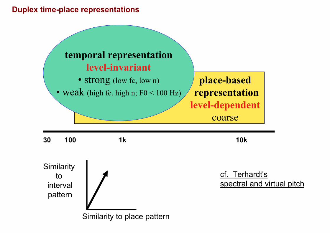
Duplex time-place representations

temporal representation

level-invariant

• strong (low fc, low n)

• weak (high fc, high n; F0 < 100 Hz)

place-based

representation

level-dependent

coarse

30 100 1k 10k

Similarity cf. Terhardt'sto spectral and virtual pitchinterval

pattern

Similarity to place pattern

Pitch dimensions: height & chroma

C6 C6

G5

G4

G3

E3

E4

E5C5

C4

C3

C5

C4

C3

Contrast between one-dimensional and two-dimensional models of pitchperception. Notes of a scale played on an ordinary instrument spiral upward around the surface of a cylinder, but computer-generated notes can form a Shepard scale that goes around in circle.

ChromaTo

ne-h

eigh

t

Pitch height and pitch chroma

Please see figures 1, 2, and 7 in Roger N. Shepard.

Geometrical approximations to the structure of musical pitch.

Psychological Review 89 (4): 305-322, 1982.

JND's

Typical human performance for pure-tone frequency discrimination.

10-2

10-3

10-4

10-5

10-6

101

100

10-1

10-2

10-3

0.2 1.0 10.0 4 10 100 500 0 10

Human

20 3040506070 80

Diff

eren

ce L

imen

( f

in H

z)

Web

er F

ract

ion

( f/

f)

Frequency (kHz) Duration (ms) Level (dB SL)

Pure tone pitch discrimination

becomes markedly worse

above 2 kHz

Weber fractions for

frequency (¨f/f) increase

1-2 orders of magnitude

between 2 kHz and 10 kHz

10-2

10-3

10-4

10-5

10-60.2 1.0 10.0

Web

er F

ract

ion

( f/

f)

Frequency (kHz)

Human

HumanData

Pure tone

pitch

discrimination

improves

at longer

tone

durations

and

at

higher

sound

pressure

levels

101

100

10-1

10-2

10-3

4 10 100 500 0 10

Human

HumanData

3

HumanData

20 3040506070 80

Diff

eren

ce L

imen

( f

in H

z)

Duration (ms) Level (dB SL)

d / Tα

d / Tα

Note durations in music

50

Overall

Image adapted from: McAdams, and Bigand. Thinking in Sound: The Cognitive Psychology of Human Audition. Oxford University Press, 1993.

Skip To

Happy Birthday

Yankee Doodle

Love Me Tender

Camptown Races

God Rest Ye Merry

Twinkle Twinkle

Rock-A-Bye Baby

100 200 500 1000 2000 5000Milliseconds

Timbre: a multidimensional tonal quality

(Photo Courtesy of Pam Roth.tone texture, tone colordistinguishes voices,

instruments

Stationary Dynamic

Aspects Aspects

Photo Courtesy of Per-Ake

Bystrom.(spectrum) ¨ spectrum

¨ intensity

¨ pitch Vowels attack

decay

Photo Courtesy of Miriam

Lewis.Consonants

http://www.wikipedia.org/

Used with permission.)

Used with permission.)

Used with permission.)

Stationary spectral aspects of timbreWaveforms Power Spectra Autocorrelations

Formant-related Pitch periods, 1/F0

[ae]

F0 = 100 Hz

[ae]

F0 = 125 Hz

[er]

F0 = 100 Hz

[er]

F0 = 125 Hz

Vowel quality Timbre

100 Hz 125 Hz

0 10 20 0 1 2 3 4 0 5 10 15

Time (ms) Frequency (kHz) Interval (ms)

Timbre dimensions: spectrum, attack, decay

Series of figures from Handel, S. 1989. Listening: an Introduction to the Perception of Auditory Events. MIT Press. Used with permission.

Masking (tone vs. tone)

Demonstration: tones in noise; tones vs. tones

Masking audiograms

Wegel & Lane, 1924

1000 Hz pure tone masker

Please see http://www. zainea.com/masking2.htm for a

discussion of masking.

Tone on tone masking curves (Wegel & Lane, 1924)

From masking patterns

to "auditory filters" as a

model of hearing

Power spectrumFilter metaphor

Notion of one central

spectrum that subserves

perception of pitch, timbre,

and loudness

2.2. Excitation pattern Using the filter shapes and bandwidths derived from masking

experiments we can produce the excitation pattern produced by a sound. The excitation pattern

shows how much energy comes through each filter in a bank of auditory filters. It is analogous to

the pattern of vibration on the basilar membrane. For a 1000 Hz pure tone the excitation pattern

for a normal and for a SNHL (sensori-neural hearing loss) listener look like this: The excitation

pattern to a complex tone is simply the sum of the patterns to the sine waves that make up the

complex tone (since the model is a linear one). We can hear out a tone at a particular frequency

in a mixture if there is a clear peak in the excitation pattern at that frequency. Since people

suffering from SNHL have broader auditory filters their excitation patterns do not have such clear

peaks. Sounds mask each other more, and so they have difficulty hearing sounds (such as

speech) in noise. --Chris Darwin, U. Sussex, http://www.biols.susx.ac.uk/home/Chris_Darwin/Perception/Lecture_Notes/Hearing3/hearing3.html

(Courtesy of Prof. Chris Darwin (Dept. of Psychology at theUniversity of Sussex). Used with permission.)

Shapes of perceptually-derived "auditory filters" (Moore)

0 c

b

d

a

ee

d

c

b

a

-10

-20

-30

-40

-50

0

-10

-20

-30

-40

-500.5 1.0 1.5 2.0 0.5 1.0 1.5 2.0

90

80

70

60

50

40

30

20

10

00.5 1 2 5 10

Rel

ativ

e ga

in, d

B

Rel

ativ

e E

xcita

tion

Leve

l, dB

Frequency, kHz Filter Center Frequency, kHzFrequency, kHz (log scale)

Exc

itatio

n Le

vel,

dB

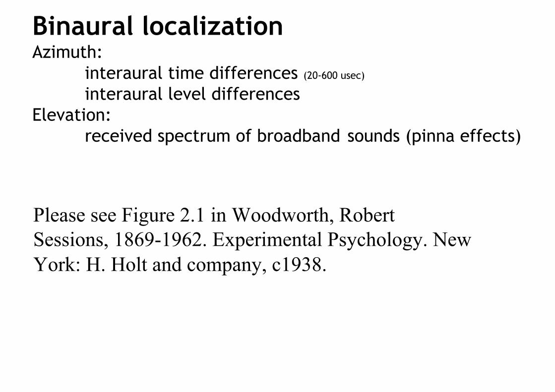
Binaural localizationAzimuth:

interaural time differences (20-600 usec)

interaural level differences

Elevation:

received spectrum of broadband sounds (pinna effects)

Please see Figure 2.1 in Woodworth, Robert

Sessions, 1869-1962. Experimental Psychology. New

York: H. Holt and company, c1938.

Interaural time difference and localization of sounds

0.6

0.5

0.4

0.3

0.2

0.1

00o 20o 40o 60o 80o 100o 120o 140o 160o 180o

Inte

raur

al T

ime

Diff

eren

ce (m

sec)