What is the precise role of non-commutativity in Quantum Theory?
28
What is the precise role of non-commutativity in Quantum Theory? B. J. Hiley. Theoretical Physics Research Unit, Birkbeck, University of London, Malet Street, London, WC1E 7HX. [[email protected]]
description
What is the precise role of non-commutativity in Quantum Theory?. B. J. Hiley. Theoretical Physics Research Unit, Birkbeck, University of London, Malet Street, London, WC1E 7HX. [[email protected]]. Non-commutativity. We know. The uncertainty principle: - PowerPoint PPT Presentation
Transcript of What is the precise role of non-commutativity in Quantum Theory?

What is the precise role of non-commutativity in Quantum Theory?
B. J. Hiley.Theoretical Physics Research Unit, Birkbeck, University of
London, Malet Street, London, WC1E 7HX.[[email protected]]

Non-commutativity.We know
€
[X, P]= ih ⇒ ΔXΔP ≈ h.
The uncertainty principle:You cannot measure X and P simultaneously.
But is it just non-commutativity?
Rotations don’t commute in the classical world.
It is not non-commutativity per se

Eigenvalues.It is when we take eigenvalues that we get trouble.
€
X x = x xP p = p p
€
But not x, p
€
Sx x + = + x +Sz z + = + z +
€
But not x+, z +
But the symmetries are carried by operators and not eigenvalues.
X, P Heisenberg group
Sx, Sz Rotation groupThe dynamics is in the operators
€
i dAdt
= [A,H ] Heisenberg’s equation ofmotion.

Symbolism.Introduce symbols
andi j
To represent
€
i
€
j
And any operator can be written as
€
A = xij i∑ j
€
(1) i j →(2) i j → operator.
C
We know these satisfy
Thus we can form
ori i i j
Complex number Matrix.

Expectation values.
€
A ji =
i j
€
trace A = Aii∑ = i j
Call
€
trace MA = i j
But this is just
€
=M jii j
i i
€
= ψ A ψ
[Lou Kauffman Knots and Physics (2001)][Bob Coecke Växjö Lecture 2005]
Pure state
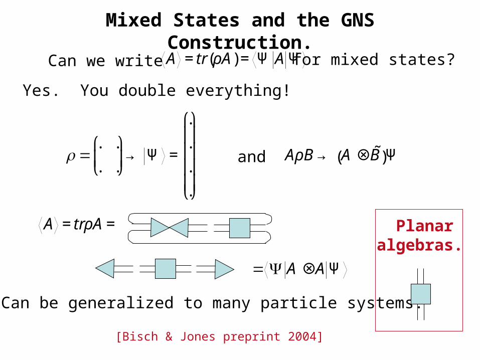
Mixed States and the GNS Construction.Can we write
€
A = tr(ρA) = Ψ A Ψ for mixed states?
Yes. You double everything!
€
ρ =. .. . ⎛ ⎝ ⎜
⎞ ⎠ ⎟→ Ψ =
.
.
.
.
⎛
⎝
⎜ ⎜ ⎜ ⎜
⎞
⎠
⎟ ⎟ ⎟ ⎟
€
AρB → A⊗ ˜ B ( )Ψand
€
A = trρA =
€
= Ψ A⊗A Ψ
Can be generalized to many particle systems.
[Bisch & Jones preprint 2004]
Planaralgebras.
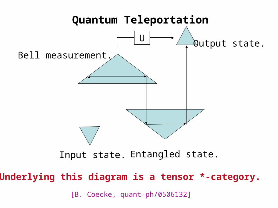
Quantum Teleportation
Underlying this diagram is a tensor *-category.
[B. Coecke, quant-ph/0506132]
Input state. Entangled state.
Bell measurement.Output state.U

Elements of Left and Right ideals.1 two-sided object splits into 2 one-sided objects.
€
Aji = i j i j
Left ideal Right ideal
Algebraically the elements of the ideals are split byan IDEMPOTENT.
€
→ e with e2 = e
Left ideal
€
ˆ Ψ L = ˆ A e Right ideal
€
ˆ Ψ R = e ˆ A
i j j i ji
This are just spinors.

Examples.
Spinors are elements of a left ideal in Clifford algebra
Symplectic spinors are elements of left ideal in Heisenberg algebra
€
ˆ Ψ L ˆ Ψ R = ˆ X =t + z x − iyx + iy t − z ⎛ ⎝ ⎜
⎞ ⎠ ⎟
Algebraic equivalent of wave function.
Everything is in the algebra.
Rotation Group.
k n
€
ˆ Ψ L ˆ Ψ R = i k n j
€
= ˆ X = i j
Symplectic Group.

Eigenvalues again.
Find in two ways.
(1) Diagonalising operator. Find spectra.
(2) Use eigenvector.i
€
X x = x x
€
i d ψdt
= H ψetc. and
But we also have
€
−i d ψdt
= ψ H
€
x X = x x etc. and
Anything new? Why complex? Why double?
i j

Now for something completely different!You can do quantum mechanics with sharply defined x and p!
€
Use ψ = Rexp[iS] in Schrödinger equation.Bohm model.
Real part gives:-
€
∂S∂t
+ ∇S( )2
2m+ ∇2R
2mR+V = 0
Quantum Hamilton-Jacobi
€
If p =∇S and E = −∂S∂t
this becomes
€
E = p2
2m+Q +V Conservation of
Energy.
New quality of energy Why?Quantum potential energy
[Bohm & Hiley, The Undivided Universe, 1993]

Probability.
Imaginary part of the Schrödinger equation gives
€
∂P∂t
+∇. P∇Sm
⎛ ⎝ ⎜ ⎞
⎠ ⎟= 0
Conservation of Probability.€
where P = R2
Start with quantum probability end with quantum probability.
Predictions identical to standard quantum mechanics.

Bohm trajectories
Screen
Slits
Incidentparticles
x
t
Barrier x
tBarrier

Wigner-Moyal Approach.
€
A = A X, P( )∫ f X, P,t( )dXdP = ψ ˆ A ψ
€
f X,P( ) = 1
2πψ ∗ X −ηh 2( )e− iηPψ∫ X +ηh 2( )dη
€
A X, P( ) = 1
2π( )2eiηP∫ ψ∗(X − ηh / 2) ˆ A ψ (X + ηh / 2)dηdX
€
ˆ A = 1
(2π )2
ψ * x, t( )∫ A X, P( )ei [ π ( ˆ x − X )+η ( ˆ p −P )]ψ (x,t )dηdπdXdPdx
Find probability distribution f (X, P, t) so that expectation value
Expectation value identical to quantum valueNeed relations
[C. Zachos, hep-th/0110114]
Problem: f (X, P, t) can be negative.
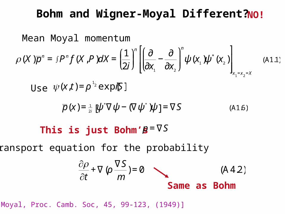
Bohm and Wigner-Moyal Different?
€
ρ(X)p n = P n f (X,P)dX = 12i ⎛ ⎝ ⎜ ⎞
⎠ ⎟∫n ∂
∂x1
− ∂∂x2
⎛ ⎝ ⎜
⎞ ⎠ ⎟n
ψ (x1 )ψ*(x2 )
⎡
⎣ ⎢ ⎢
⎤
⎦ ⎥ ⎥x1 =x2 =X
(A1.1)
€
p (x) = 12 i ψ *∇ψ − (∇ψ * )ψ[ ] =∇S (A1.6)
€
∂ρ∂t
+∇(ρ ∇Sm
) = 0 (A4.2)
NO!
Mean Moyal momentum
€
ψ(x,t) = ρ 12 exp[iS]Use
This is just Bohm’s
€
p =∇S
Transport equation for the probability
[J. E. Moyal, Proc. Camb. Soc, 45, 99-123, (1949)]
Same as Bohm

Transport equation for
This is Bohm’s quantum Hamilton-Jacobi equation.
p
€
∂∂t
ρp ( ) + ∂∂xi
ρpk
∂H ∂x1
⎛ ⎝ ⎜
⎞ ⎠ ⎟+ ρ ∂H
∂xki
∑ = 0 (A4.3)
€
∂∂xk
∂S∂t
+ H −∇ρ 8mρ ⎡ ⎣ ⎢
⎤ ⎦ ⎥= 0 (A4.5)
€
∂S∂t
+ H −∇ρ 8mρ = ∂S∂t
+ 1
2m(∇S)2 +V − 1
2m∇ 2R R = 0
€
p Transport equation for
Which finally gives

Moyal algebra is deformed Poisson algebra• Define Moyal product *
• Moyal bracket(commutator)
• Baker bracket (Jordan product or anti-commutator)
• Classical limit Sine becomes Poisson bracket.
• Cosine becomes ordinary product.
A,B{ }MB =A∗B−B∗A
ih =2A(X,P)sinh2
s ∂
∂X
r ∂ ∂P
−r ∂
∂X
s ∂ ∂P
⎡ ⎣ ⎢ ⎢
⎤ ⎦ ⎥ ⎥ B(X,P)
A,B( )BB =A∗B+B∗A
2 =A(X,P)cosh2
s ∂
∂X
r ∂
∂P−
r ∂
∂X
s ∂
∂P⎡ ⎣ ⎢ ⎢
⎤ ⎦ ⎥ ⎥ B(X,P)
A∗B =A X,P( )eih2
s ∂ ∂x
r ∂ ∂p
−r ∂ ∂x
s ∂ ∂p
⎡ ⎣ ⎢ ⎢
⎤ ⎦ ⎥ ⎥ B(X,P)
A,B{ }MB = A,B{ }PB +O(h2) ≈ ∂A
∂X∂B∂P
−∂A∂P
∂B∂X
⎡ ⎣ ⎢
⎤ ⎦ ⎥
A,B{ }BB =AB+O(h2)
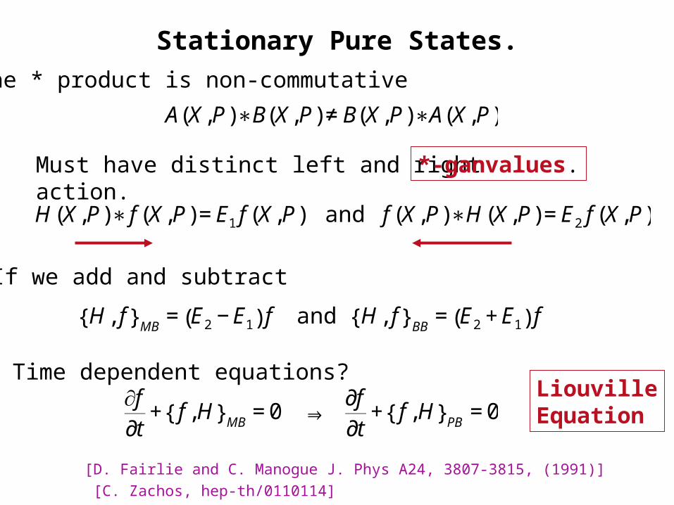
Stationary Pure States.
[D. Fairlie and C. Manogue J. Phys A24, 3807-3815, (1991)] [C. Zachos, hep-th/0110114]
€
H (X,P)∗ f (X,P) = E1 f (X,P) and f (X,P)∗H (X, P) = E2 f (X,P)
€
H , f{ }MB = E2 − E1( ) f and H , f{ }BB = E2 + E1( ) f
€
∂f∂t
+ f , H{ }MB = 0 ⇒ ∂f∂t
+ f , H{ }PB = 0
The * product is non-commutative
€
A(X,P)∗B(X, P) ≠ B(X,P)∗A(X,P)
Must have distinct left and right action.
If we add and subtract
Time dependent equations?LiouvilleEquation
*-ganvalues.

The ‘Third’ Equation
[D. Fairlie and C. Manogue J. Phys A24, 3807-3815, (1991)]
€
H ∗ f = i2π dηe−iηpψ∗(x −η 2)∂ψ (x +η 2)
∂t∫
€
f ∗H = − i2π dηe−iηp ∂ψ∗(x −η 2)
∂t∫ ψ (x +η 2)
€
H ∗ f + f ∗H = i2π dηe−iηp ψ∗(x −η 2)∂ψ (x +η 2)
∂t−∂ψ∗(x −η 2)
∂tψ (x +η 2)
⎡ ⎣ ⎢
⎤ ⎦ ⎥∫
Need Left and Right ‘Schrödinger’ equations. Try
and
Difference gives Liouville equation.
€
∂f∂t
+ f , H{ }MB = 0 ⇒ ∂f∂t
+ f , H{ }PB = 0
Sum gives ‘third’ equation.
???
€
(h =1)

Third equation is Quantum H-J.
[B. Hiley, Reconsideration of Foundations 2, 267-86, Växjö, 2003]
ψ ∗∂ψ
∂t−∂ψ ∗
∂tψ
⎡ ⎣ ⎢
⎤ ⎦ ⎥ = 1
R(x+hη 2)∂R(x+hη 2)
∂t− 1
R(x−hη 2)∂R(x−hη 2)
∂t⎡ ⎣ ⎢
⎤ ⎦ ⎥ ψ ∗ψ
+i ∂S(x+hη 2)
S(x+hη 2) +∂S(x−hη 2)S(x−hη 2)
⎡ ⎣ ⎢
⎤ ⎦ ⎥ ψ ∗ψ
€
∂S∂t
+ H = 0
€
ψ =ReiS /hSimplify by writing
Classical limit
€
H ∗ f + f ∗H = −2∂S∂t
f +O(h2 )
€
→ 2∂S∂t
f + H , f{ }BB = 0
Classical H-J equation

Same for Operators?
We have two sides.ji
and
Two symplectic spinors.
Operator equivalent of Wave Function
€
ˆ ψ L
= ˆ A ε
€
ˆ ψ R =ε ˆ B Operator equivalent of conjugate WF
Two operator Schrödinger equations
€
i ∂ ˆ ψ L∂t
= ˆ H ˆ ψ L and − i ∂ ˆ ψ R∂t
= ˆ ψ R ˆ H

The Two Operator Equations.
[Brown and Hiley quant-ph/0005026]
€
ir ∂ ∂t
ˆ ψ L ⎛ ⎝ ⎜
⎞ ⎠ ⎟ˆ ψ R + ˆ ψ L ˆ ψ R
s ∂ ∂t
⎛ ⎝ ⎜
⎞ ⎠ ⎟
⎡ ⎣ ⎢
⎤ ⎦ ⎥= ˆ
r H ˆ ψ L( ) ˆ ψ R − ˆ ψ L ˆ ψ R ˆ
s H ( )
€
With ˆ ρ = ˆ ψ L ˆ ψ R
€
i ∂ ˆ ρ ∂t
+ ˆ ρ , ˆ H [ ] −= 0
€
ir ∂ ∂t
ˆ ψ L ⎛ ⎝ ⎜
⎞ ⎠ ⎟ˆ ψ R − ˆ ψ L ˆ ψ R
s ∂ ∂t
⎛ ⎝ ⎜
⎞ ⎠ ⎟
⎡ ⎣ ⎢
⎤ ⎦ ⎥= ˆ
r H ˆ ψ L( ) ˆ ψ R + ˆ ψ L ˆ ψ R ˆ
s H ( )
€
ˆ ψ L = ˆ R ei ˆ S ε and ˆ ψ R = εei ˆ S ˆ R
€
ˆ ρ ∂ˆ S
∂t+ 1
2ˆ ρ , ˆ H [ ] +
= 0
Sum
Quantum Liouville
Difference
New equation

The Operator Equations.
€
i ∂ ˆ ρ ∂t
+ ˆ ρ , ˆ H [ ] −= 0
€
ˆ ρ ∂ˆ S
∂t+ 1
2ˆ ρ , ˆ H [ ] +
= 0
€
2∂S∂t
f + f , H{ }BB = 0€
∂f∂t
+{ f , H}MB = 0
Wigner-Moyal Quantum
Where is the quantum potential?

Projection into a Representation.
[Brown and Hiley quant-ph/0005026]
€
i dP(a)dt
+ ˆ ρ , ˆ H [ ] − a= 0
€
P(a)∂S(a)∂t
+ 12 ˆ ρ , ˆ H [ ] + a
= 0
€
ˆ H = ˆ p 2
2m+ K ˆ x 2
2€
∂P∂t
+∇. P∇Sm
⎛ ⎝ ⎜ ⎞
⎠ ⎟= 0
€
∂Sx
∂t+ 1
2m∂Sx
∂x ⎛ ⎝ ⎜ ⎞
⎠ ⎟2
+ Kx 2
2− 1
2mRx
∂2Rx
∂x 2
⎛ ⎝ ⎜
⎞ ⎠ ⎟= 0
Project into representation using
€
Pa = a a
Still no quantum potential
Choose
€
Px = x x
Conservation of probability
Quantum H-J equation.
Out pops thequantum potential

The Momentum Representation.
Trajectories from the streamlines of probability current.€
∂Sp
∂t+ p 2
2m+ K
2∂Sp
∂p ⎛ ⎝ ⎜
⎞ ⎠ ⎟2
− K2Rp
∂2Rp
∂p 2
⎛ ⎝ ⎜
⎞ ⎠ ⎟= 0
€
∂Pp
∂t+
∂j p
∂p= 0
€
j p = − p ∂( ˆ ρ V ( ˆ x ))∂x
p
Choose
€
Pp = p p
€
x = −∂Sp
∂p ⎛ ⎝ ⎜
⎞ ⎠ ⎟But now
Possibility of Bohm model in momentum space.
Returns the x p symmetry to Bohm model.

Shadow Phase Spaces.
[M. R. Brown & B. J. Hiley, quant-ph/0005026][B.Hiley, Quantum Theory:Reconsideration of Foundations, 2002, 141-162.]
x p
pr = Re(ψ*Pψ) xρ = Re(ψ*Xψ)
OR
Non-commutative quantum algebra implies no unique phase space.
Project on to Shadow Phase Spaces.
Quantum potential is an INTERNAL energy arising from
projection into a classical space-time.

General structure.
Shadow phase spaces
Non-commutativeAlgebraic structure.
Shadowmanifold
Shadowmanifold
Shadowmanifold
€
B = H + Qψ
€
B = H + Qφ
€
B = H + Qη
Guillemin & Sternberg, Symplectic Techniques in Physics 1990.Abramsky & Coecke quant-ph/0402130Baez, quant-ph/0404040
Covering space Sp(2n) ≈ Ham(2n)
A general *-algebra
Monoidal tensor *-category

The Philosophy.
Non-commutativeAlgebraic structure.
Implicate order.
Holomovement
Shadowmanifold
Shadowmanifold
Shadowmanifold
€
B = H + Qψ
€
B = H + Qφ
€
B = H + Qη
Possible explicate orders.[D. Bohm Wholeness and the Implicate Order (1980])