1

What is Quantum Mechanics?

QM is the theoretical framework that we use to describe the behaviour of particles, nuclei, atoms, molecules and condensed matter.

Elementary particles are characterized by a set of ‘numbers’, e.g. charge and spin, whose values are discrete: these are called ‘quantum numbers’.

Discreteness was not found first in the microcosm. Vibrating bodies, e.g. strings, have discrete frequencies, which seems to be the result of boundary conditions. Similarly, bound quantum systems, e.g. atoms, have discrete energy levels.

2

The quantum

The values of quantized quantities are multiples of a minimum amount: the quantum of the related quantity.

The quantum of energy of radiation of frequency v isE=hv

All quanta are proportional to the Planck constant, h=6.62x10-34 Js. If h=0, quantum and classic physics would coincide.

3

Wave-particle duality

The relation E=hv implies that waves behave like ‘bunches’ of energy, i.e. they exhibit particle-like nature. Particles have also shown wave-like behaviour, e.g. electron beams hitting a double-slit give rise to interference phenomena.

RAF211 - CZJ 4

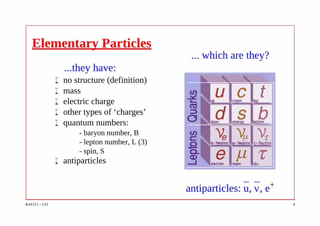
Elementary Particles

...they have:w no structure (definition)w massw electric chargew other types of ‘charges’w quantum numbers:

- baryon number, B- lepton number, L (3)- spin, S

w antiparticles

... which are they?

antiparticles: u, ν, e+

RAF211 - CZJ 5

Fundamental Interactions

RAF211 - CZJ 6

The mediatorsq The interactions occurs by the

exchange of mediators:

l strong: gluons, g (8)l e/m: photon, γl weak: Z, W+, W−

l gravity: graviton

e/m force:

strong force:

γ

RAF211 - CZJ 7

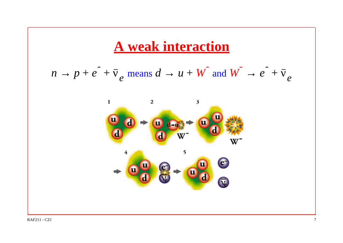
A weak interaction

means and n p e- νe+ +→ d u W

-+→ W

-e

- νe+→

RAF211 - CZJ 8

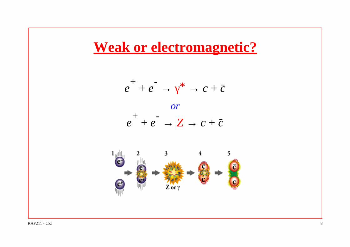
Weak or electromagnetic?

or

e+

e-

+ γ∗ c→ c+→

e+

e-

+ Z c→ c+→

RAF211 - CZJ 9

Fundamental interactions: properties

interactionrelative strength

time rangeparticipating

particles

strong 1 10-23 s 10-15 m quarks (gluons)

e/m 0.01 10-20 s infinite electrically charged (γ)

weak 0.00001 10-8 s 10-18 m all

(Z0,W+,W-)

RAF211 - CZJ 10

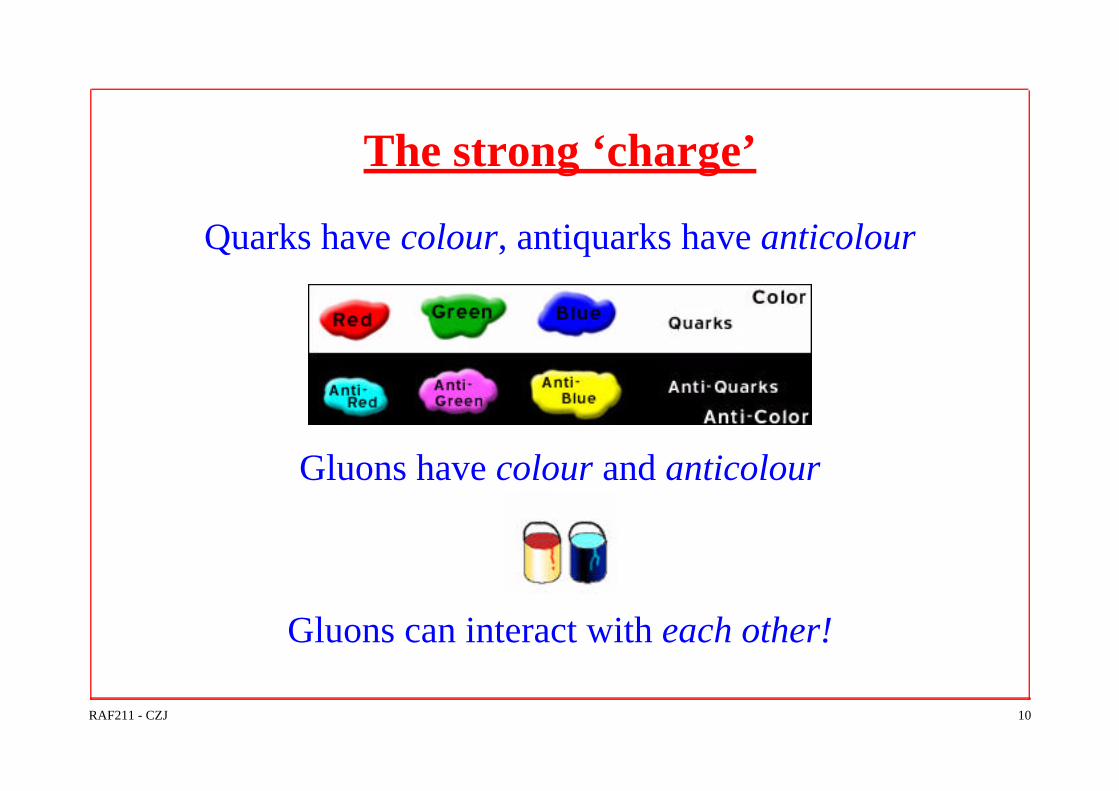
The strong ‘charge’

Quarks have colour, antiquarks have anticolour

Gluons have colour and anticolour

Gluons can interact with each other!

RAF211 - CZJ 11

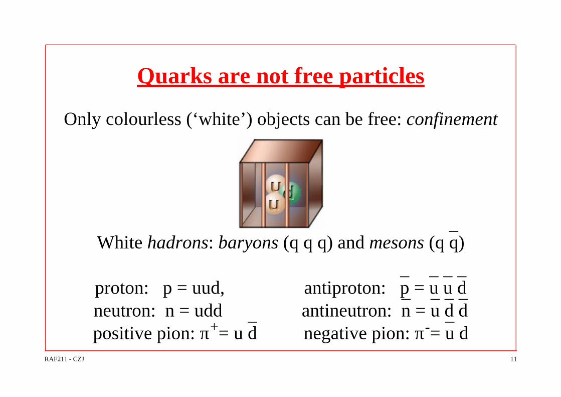
Quarks are not free particles

Only colourless (‘white’) objects can be free: confinement

White hadrons: baryons (q q q) and mesons (q q)

proton: p = uud, antiproton: p = u u dneutron: n = udd antineutron: n = u d dpositive pion: π+= u d negative pion: π-= u d

RAF211 - CZJ 12

What happens if we pull two quarks apart?

hadronization

RAF211 - CZJ 13

Quantum Numbers

Quarks: B = 1/3, L = 0, S = 1/2,Q=2/3 (up) or -1/3 (down)

Leptons:B = 0, L = 1, S = 1/2,Q = -1 or 0 (neutrinos)

Antiparticles: opposite quan-tum numbers (but same spin)

Conservation laws

strong E/M weak

energy ☺☺ ☺☺ ☺☺

momentum ☺☺ ☺☺ ☺☺

electric charge ☺☺ ☺☺ ☺☺

spin ☺☺ ☺☺ ☺☺

Baryon # ☺☺ ☺☺ ☺☺

Lepton # ☺☺ ☺☺ ☺☺

Parity ☺☺ ☺☺ LL

RAF211 - CZJ 14

The muon decay

electron lepton number, Le: 0 = 1 + (-1) + 0

muon lepton number, Lµ: 1 = 0 + 0 + 1

tau lepton number, Lτ: 0 = 0 + 0 + 0

µ e- νe νµ+ +→

RAF211 - CZJ 15

The residual effects of the forces

...which acts between elementary particles, but we see this:

...and this:

residual

residual

e/m force

strong force

1

Special relativity

It was assumed that light, like mechanical waves, propagates in a medium, called the ether, at the velocity c=3x108 m/s and has different velocities at other reference systems

1887: Michelson-Morley tried to measure the velocity of ether with respect to Earth but the experiment found no evidence of such a medium

1905: Einstein presents the postulates of the special theory of rela-tivity:- the laws of physics are the same in all inertial reference frame- the speed of light in free space is c in all inertial reference frames

2

Time dilation

Let us assume two reference frames (or observers), A and B, which are in relative motion. We assume that both observers use cartesian coordinate systems, (xA,yA,zA) and (xB,yB,zB), which coincide at t=0. The observer B then starts moving in the positive x direction at a velocity (u,0,0) with re-spect to the observer A.

If something happens at rest in B and has a duration of , the observerin A will measure time

∆t0

∆t∆t0

1 u2

c2

⁄–

---------------------------- γ∆t0= =

3

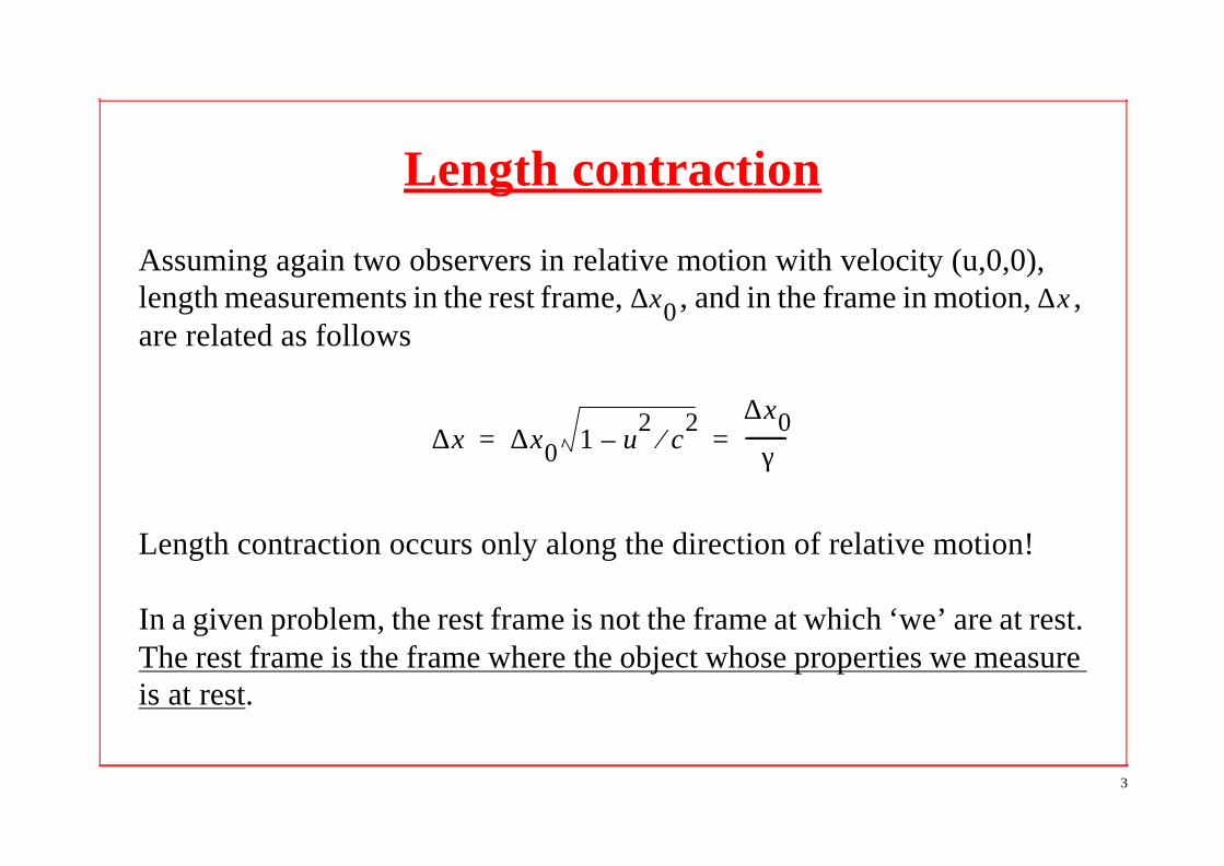
Length contraction

Assuming again two observers in relative motion with velocity (u,0,0), length measurements in the rest frame, , and in the frame in motion, , are related as follows

Length contraction occurs only along the direction of relative motion!

In a given problem, the rest frame is not the frame at which ‘we’ are at rest. The rest frame is the frame where the object whose properties we measure is at rest.

∆x0 ∆x

∆x ∆x0 1 u2

c2

⁄–∆x0

γ---------= =

4

Relativistic momentum and energy

The relativistic momentum of a particle with nonzero rest mass moving at a velocity is given by

The rest energy of a particle is determined by its rest mass

The total energy of a particle is given by

The kinetic energy of the particle is then .

A useful relation: ( for a massless particle)

m0v

pm0v

1 v2

c2

⁄–

---------------------------- γm0v= =

E0 m0c2

=

E mc2

γm0c2

= =

K E E0–=

E pc( )2

m0c2

( )2

+= p E c⁄=

RAF211 - CZJ 16

How does the microcosm ‘move’?

In classical mechanics, we have:

- observables: p, v, x, ... - parameter: t - Newton’s law: F=ma - equation of motion: x(t)

The observables take continuous values

Is it so in the microcosm?

RAF211 - CZJ 1

Quantum Mechanics

(non-relativistic)4 basics4 operators4 momentum eigenstates4 energy eigenstates

RAF211 - CZJ 2

Some basic notions

4object: what we study (particle, atom, ...)4observable: a measurable property of the object (E, p, ...)4parameter t: this ‘time’ is not a property of the object4state of an object: the values of its observables 4wavefunction: the mathematical expression of a state, e.g.

We use the wavefunctions to find the state of an object , i.e. to find the value of its observables. How is this done?

ψ x( ) x( )sin=k

RAF211 - CZJ 3

Operators (‘type 1’)

an operator is something that can be applied to a mathematical function and give a mathematical function

e.g. is an operator:

Postulate of Quantum Mechanics: observables are described by operators

Ad

2

dx2

--------= Aψ 1–( ) k xsin⋅( )=

RAF211 - CZJ 4

Operators (‘type 2’)

an operator can perform a transformation( in space or in time or both)

example: the transformation

is performed by the operator (definition):

the operator is called the ‘parity operator’

x y z, ,( ) x y z–,–,–( )→

PPψ x y z, ,( ) ψ x– y– z–, ,( )=

P

RAF211 - CZJ 5

Eigenstates and eigenvalues

Assume an operator of ‘type 1’ or ‘type 2’.If , where =constant, we say that

is eigenstate of the operator with eigenvalue

4each eigenstate has only one eigenvalue4degenerate eigenvalues (common eigenvalues)4spectrum of an operator: the set of its eigenvalues4Hermitian operator: has only real eigenvalues

We use Hermitian operators to express observables

QQψ qψ= q

ψ Q q

RAF211 - CZJ 6

Example: parity eigenvalues

We apply the parity operator (transformation) twice

i.e.

If , then

i.e. = the parity of the state ( : even parity, : odd parity)

x y z, ,( ) x y z–,–,–( ) x y z, ,( )→ →P Pψ( ) ψ=

Pψ λψ=

P Pψ( ) P λψ( ) λ Pψ( ) λ λψ( ) λ2ψ ψ= = = = =

λ 1±= ψλ 1= λ 1–=

RAF211 - CZJ 7

Measurements are eigenvalues

Assume an observable , represented by the operator .We measure in a state . What will we get?

case 1: is eigenstate of with eigenvalue .result: all measurements are equal to .

case 2: is not an eigenstate of . result: a measurement will be any eigenvalue of but we cannot predict which one.

(We never use the same state to measure twice)

A AA ψ

ψ A aa

ψ A

A

RAF211 - CZJ 8

Probability interpretation

wavefunctions are normalized to unity:

this allows us to say that

is the probability to find the object at (x,x+dx)

ψ x( ) 2xd∫ 1=

P ψ x( ) 2= xd

RAF211 - CZJ 9

Indeterminacy in the position of an object

it actually means that objects can be found where we don’t expect them to be

the proton is most likely hereor it could be here

or even here

these four particlesmight migrate

outside the nucleus

the electrons arehere someplace

RAF211 - CZJ 10

Example: a particle in a box

ψ

x

x

|ψ|2

RAF211 - CZJ 1

The representation of observables

...some simple formulae for operators

RAF211 - CZJ 2

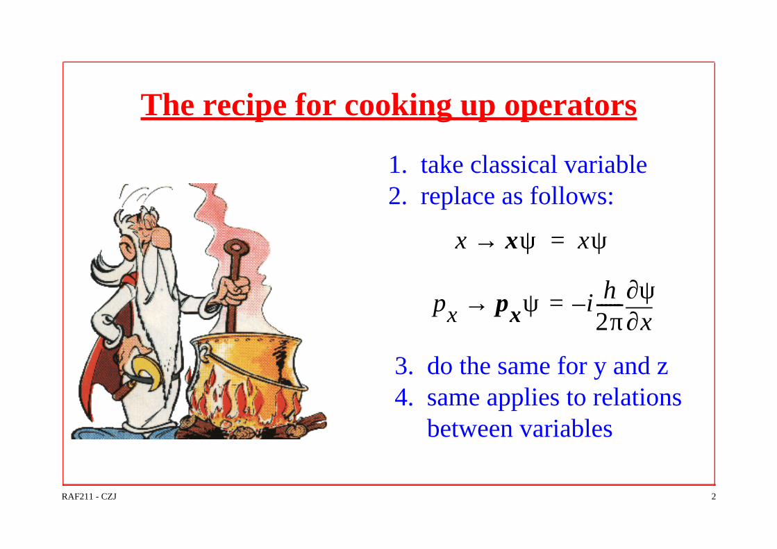
The recipe for cooking up operators

1. take classical variable 2. replace as follows:

3. do the same for y and z 4. same applies to relations between variables

x xψ→ xψ=

px pxψ i h2π------–=

x∂∂ψ→

RAF211 - CZJ 3

The position operator(s)

A vector* operator

where , and

are the component operators

* Operators of this form are not ordinary 3d vectors!

R xux yuy zuz+ +=

xψ xψ= yψ yψ= zψ zψ=

operators act only

on wavefunctions

RAF211 - CZJ 4

The linear momentum operator(s)

A vector operator

where

, and

are the component operators4 What is the operator for ?

p pxux pyuy pzuz+ +=

pxψ i h2π------–=

x∂∂ψ pyψ i h

2π------–=

y∂∂ψ pzψ i h

2π------–=

z∂∂ψ

p2

RAF211 - CZJ 5

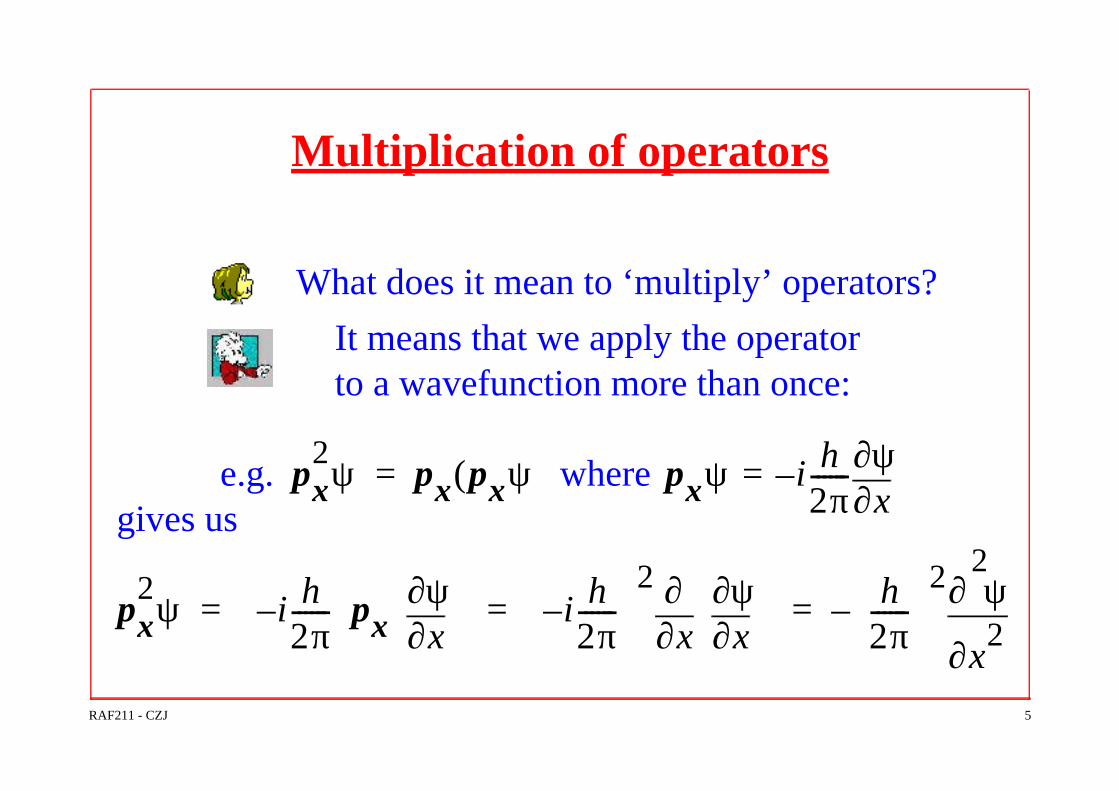
Multiplication of operators

What does it mean to ‘multiply’ operators?

It means that we apply the operator to a wavefunction more than once:

e.g. where gives us

px2ψ px pxψ( )= pxψ i h

2π------–=

x∂∂ψ

px2ψ i h

2π------–

px x∂∂ψ

i h

2π------–

2

x∂∂

x∂∂ψ

h

2π------

2

x2

2

∂

∂ ψ–= = =

RAF211 - CZJ 6

The operator for orbital angular momentum

The classical representation (variable) is , so the quantum mechanical representation (operator) will be , which gives

, ,

For example,

L r p×=

L r p×=

Lx ypz zpy–( )= Ly zpx xpz–( )= Lz xpy ypx–( )=

Lxψ ypz zpy–( )ψ ypzψ zpyψ– y pzψ( ) z pyψ( )–= = =

Lxψ i h2π------– y

z∂∂ψ z–

y∂∂ψ

=

RAF211 - CZJ 7

The kinetic energy operator

We use the formula of classical mechanics:

where

K 12m-------p

2 12m------- px

2py

2pz

2+ +( )

12m-------– h

2π------

2∇∇2

= = =

∇∇2

x2

2

∂

∂

y2

2

∂

∂

z2

2

∂

∂+ +=

RAF211 - CZJ 8

The total energy operator (when E=K+V)

We assume an object in motion (K) in a region of a potential V:

Observe that the potential operator is given by the classical variable because it depends on x, y, z

The operator is called the Hamiltonian operator(‘the Hamiltonian of the system’)

H K= V x y z, ,( )+1

2m-------– h

2π------

2∇∇2

V x y z, ,( )+=

H

RAF211 - CZJ 9

The operator E

It gives the time-dependence of energy eigenstates

By combining with the expression E=K+V, we obtain:

the time-dependent Schrödinger equation

E i h2π------

t∂∂=

i h2π------

t∂∂Ψ 1

2m-------– h

2π------

2∇∇2Ψ V+ Ψ=

RAF211 - CZJ 10

The commutator operator

Can we ‘multiply’ two operators and in any order?

We can, if their commutator is zero.

Definition of the commutator operator:

Physical meaning of :the operators and have

common (simultaneous) eigenstates

A B

A B,[ ]

A B[ , ] AB BA–=

A B[ , ] 0=A B

RAF211 - CZJ 11

Examples of commutators

1. position and momentum in the same direction:

(same relation for y and z)

2. angular momentum in different directions:

(and cyclic permutations) but

x px[ , ] i h2π------=

Lx Ly[ , ] i h2π------Lz=

L2

Lx[ , ] L2

Ly[ , ] L2

Lz[ , ] 0= = =

RAF211 - CZJ 12

Common eigenstate problem in atoms

Assume that we have an object (atom) in a potential V(r)and we are interested in states of constant total energy, E.

The following relations hold:

So we can measure simultaneously: E, L2, Lz.

x H,[ ] 0 y H,[ ] 0 z H,[ ] 0≠,≠,≠

H px[ , ] 0 H py[ , ] 0 H pz[ , ] 0≠,≠,≠

L2

H[ , ] H Lz[ , ] L2

Lz[ , ] 0= = =

RAF211 - CZJ 13

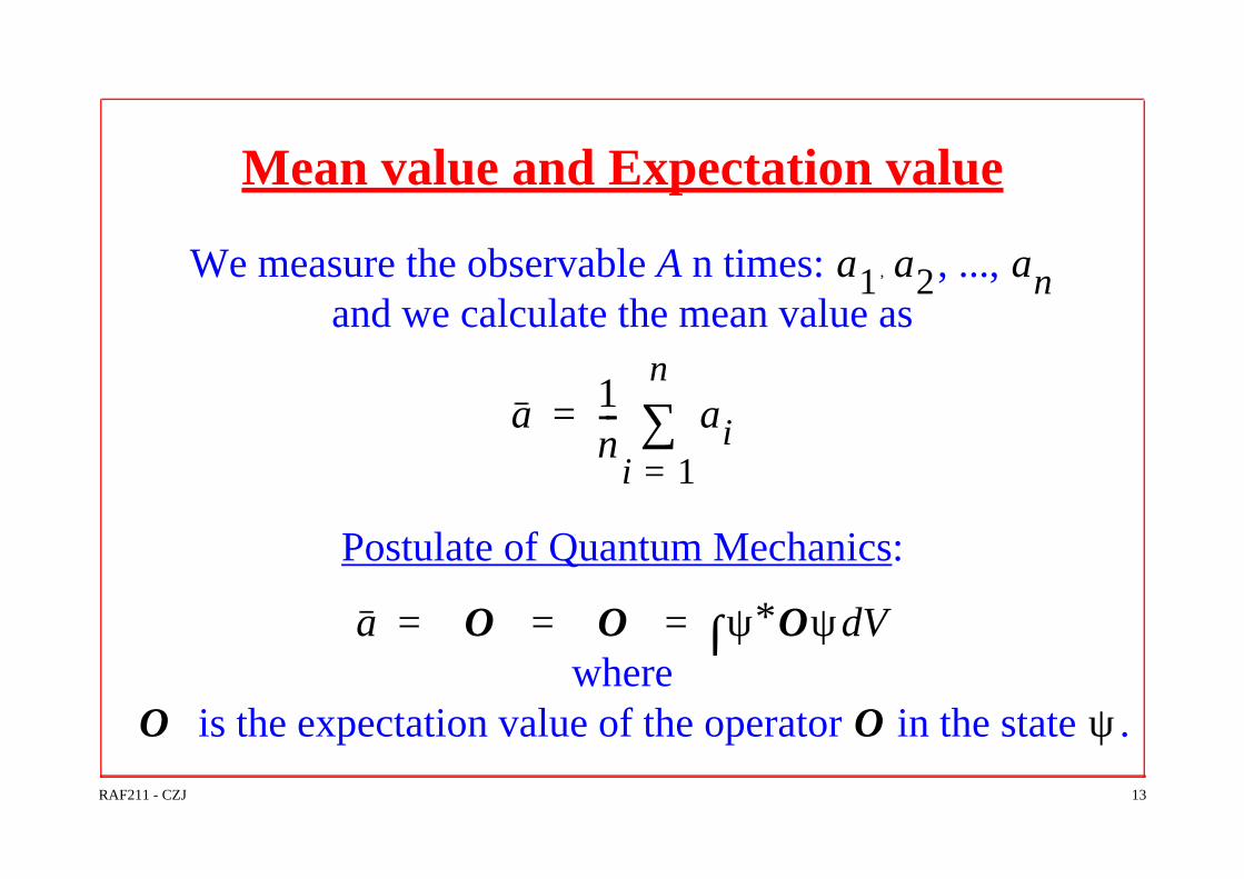
Mean value and Expectation value

We measure the observable A n times: , , ..., and we calculate the mean value as

Postulate of Quantum Mechanics:

where is the expectation value of the operator in the state .

a1 a2 an

a 1n--- ai

i 1=

n

∑=

a O⟨ ⟩ O⟨ ⟩ ψ∗Oψ Vd∫= = =

O⟨ ⟩ O ψ

RAF211 - CZJ 14

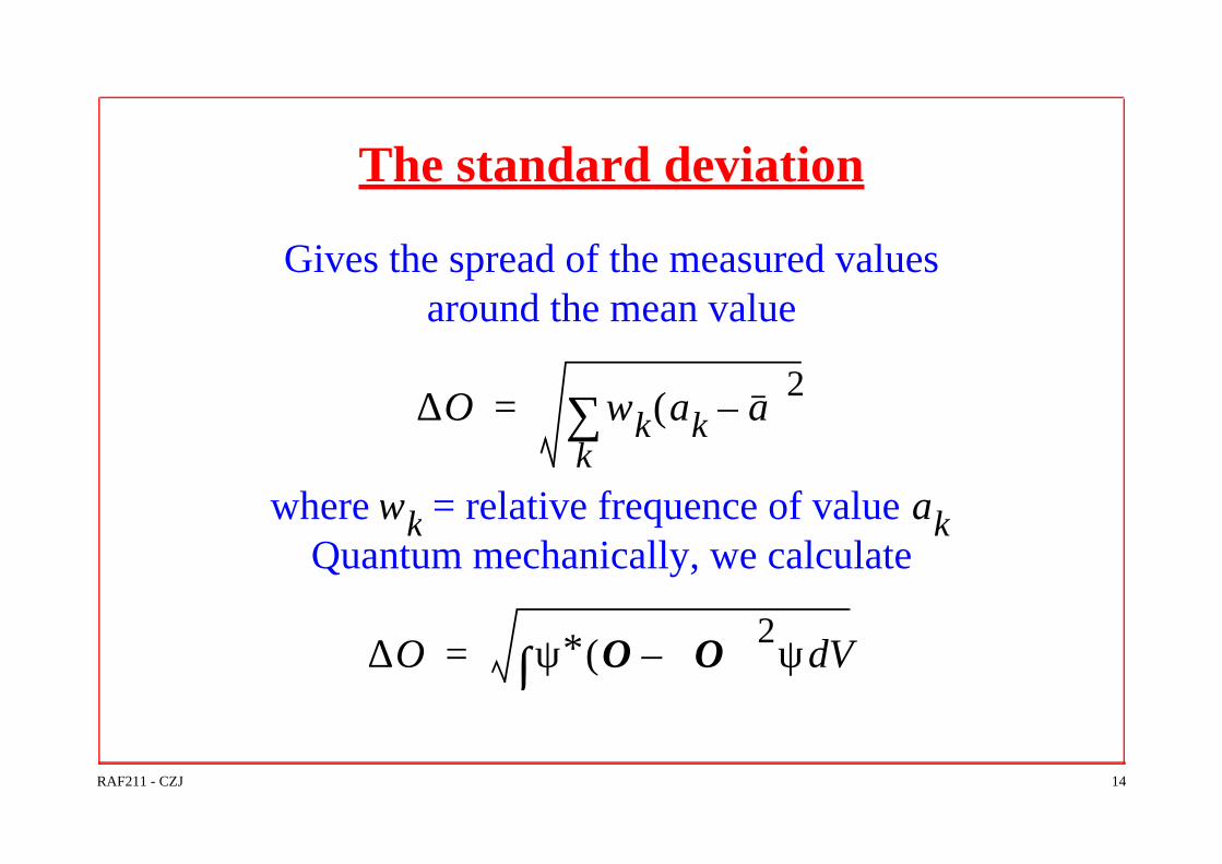
The standard deviation

Gives the spread of the measured values around the mean value

where = relative frequence of value Quantum mechanically, we calculate

∆O wk ak a–( )2

k∑=

wk ak

∆O ψ∗ O O⟨ ⟩–( )2ψ Vd∫=

RAF211 - CZJ 15

The Heisenberg principle

Assume that we measure P and Q in the state (which is not an eigenstate of their operators).

The following holds for their standard deviations:

If the operators do not commute, the right-hand side is not zero. Examples:

,

ψ

∆P( )2 ∆Q( )2 14--- ψ∗ PQ QP–( )ψ Vd∫[ ]

2–

≥⋅

∆px ∆x⋅ h 4π( )⁄= ∆E ∆t h 4π( )⁄=⋅

RAF211 - CZJ 16

Conserved Observables

An observable is conserved (i.e. its expectation value does not change with time) when its operator commutes

with the Hamiltonian (of the system we study)

Application: the angular orbital momentum of atoms is a constant of the motion

tdd O⟨ ⟩ 2πi

h-------- H O,[ ]⟨ ⟩=

RAF211 - CZJ 1

Momentum eigenstates

å linear momentum eigenstateså orbital angular momentum eigenstateså spin angular momentum eigenstateså addition of angular momenta

l the generic angular momentum operator

We will work mainly with quantum numbersin the applications

RAF211 - CZJ 2

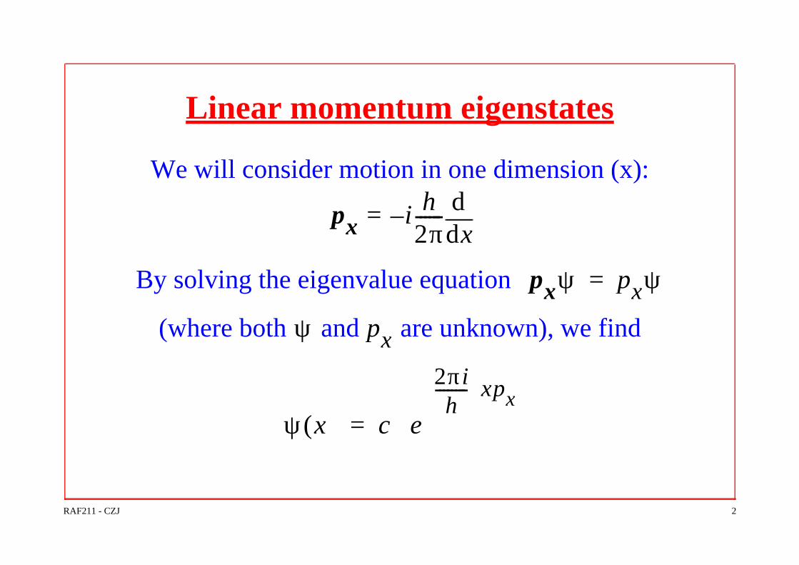
Linear momentum eigenstates

We will consider motion in one dimension (x):

By solving the eigenvalue equation

(where both and are unknown), we find

px i h2π------–=

xdd

pxψ pxψ=

ψ px

ψ x( ) c e

2πih

-------- xpx

⋅=

RAF211 - CZJ 3

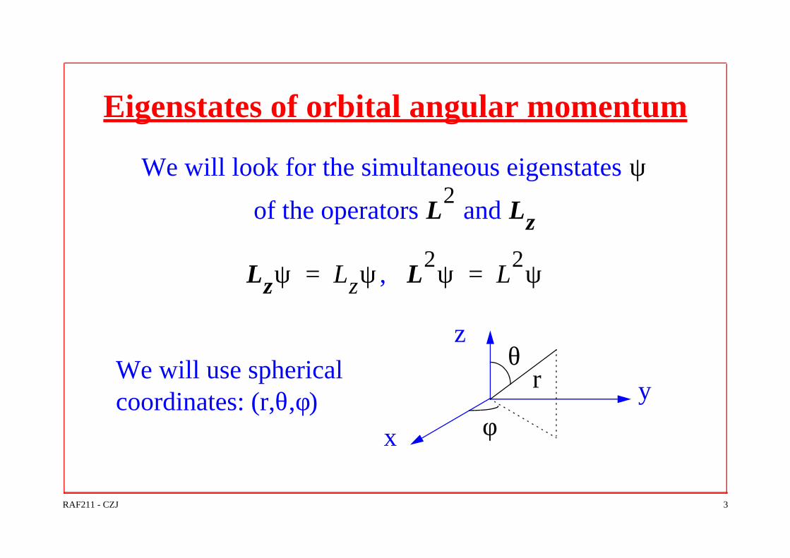
Eigenstates of orbital angular momentum

We will look for the simultaneous eigenstates

of the operators and

,

We will use spherical coordinates: (r,θ,φ)

ψ

L2

Lz

Lzψ Lzψ= L2ψ L

2ψ=

y

x

z

r

φ

θ

RAF211 - CZJ 4

Lz eigenstates and eigenvalues

The eigenvalue equation

gives

Condition:

is the magnetic quantum number

i h2π------

φddψ– Lz=

ψ φ( ) ce

2πih

-------- φLz

=

ψ φ( ) ψ φ 2π+( ) Lz m h2π------=⇒=

m 0 1 2 …,±,±,=

quantized

RAF211 - CZJ 5

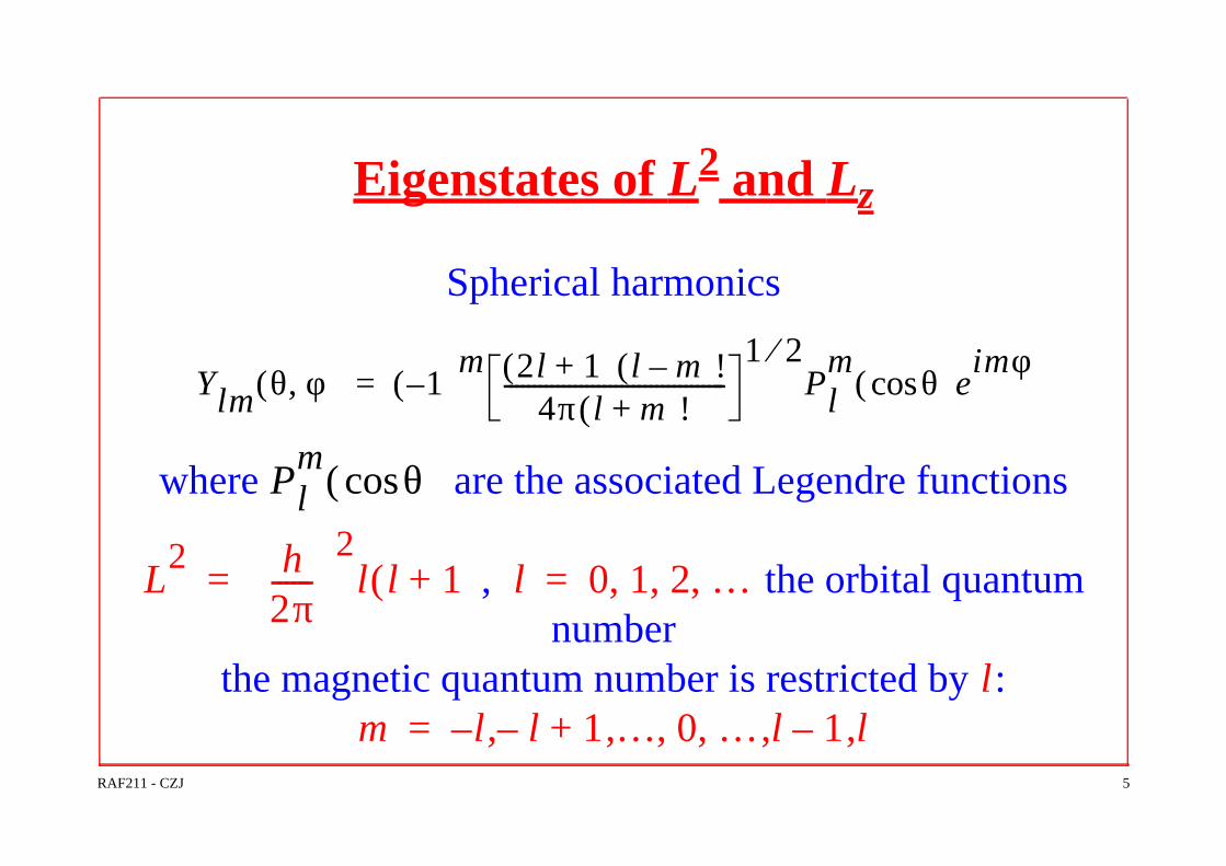
Eigenstates of L2 and Lz

Spherical harmonics

where are the associated Legendre functions

, the orbital quantum number

the magnetic quantum number is restricted by :

Ylm θ φ,( ) 1–( )m 2l 1+( ) l m–( )!

4π l m+( )!--------------------------------------

1 2⁄Pl

mθcos( )e

imφ=

Plm θcos( )

L2 h

2π------

2l l 1+( )= l 0 1 2 …, , ,=

lm l l– 1+ … 0 … l 1– l,,, ,,,–=

RAF211 - CZJ 6

Parity eigenstates

The spherical harmonics are also eigenstatesof the parity operator

Application: transitions in atoms

PYlm 1–( )lYlm=

RAF211 - CZJ 7

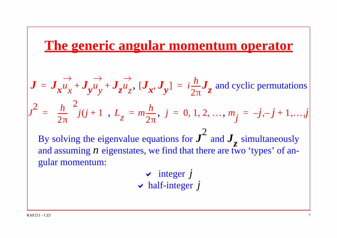
The generic angular momentum operator

, and cyclic permutations

, , ,

By solving the eigenvalue equations for and simultaneouslyand assuming eigenstates, we find that there are two ‘types’ of an-gular momentum:

a integer a half-integer

J Jxux Jyuy Jzuz+ += Jx Jy,[ ] i h2π------Jz=

J2 h

2π------

2j j 1+( )= Lz m h

2π------= j 0 1 2 …, , ,= mj j j– 1+ … j,,,–=

J2

Jzn

jj

RAF211 - CZJ 8

The spin angular momentum

Spin does not involve a rotation in space

where is the spin quantum number

,

a integer : bosonsa half-integer : fermions

S2 h

2π------

2s s 1+( )=

s

Sz msh

2π------= ms s s– 1+ … s 1– s,,,,–=

ss

RAF211 - CZJ 9

Addition of angular momenta

Let us assume that we want to ‘add’ the quantum numbers and tofind the quantum number of the total angular momentum, , and thequantum number of the z-component,

The rules are:

1. 2. for each , we have ’s:

Application: L-S coupling and J-J coupling in atoms

l sj

mj

j l s– … l s+, ,=j 2j 1+ mj mj j j– 1+ … j,,,–=

1

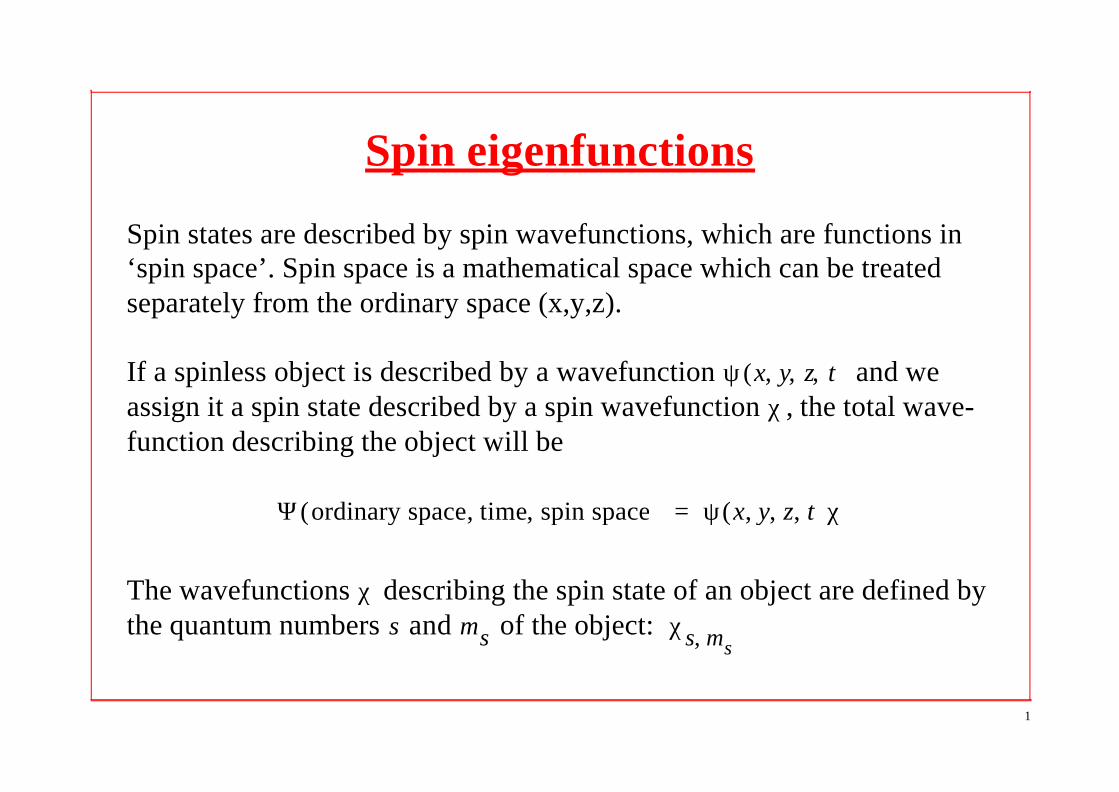
Spin eigenfunctions

Spin states are described by spin wavefunctions, which are functions in ‘spin space’. Spin space is a mathematical space which can be treated separately from the ordinary space (x,y,z).

If a spinless object is described by a wavefunction and we assign it a spin state described by a spin wavefunction , the total wave-function describing the object will be

The wavefunctions describing the spin state of an object are defined by the quantum numbers and of the object:

ψ x y z t, , ,( )χ

Ψ ordinary space time spin space, ,( ) ψ x y z t, , ,( )χ=

χs ms χs ms,

2

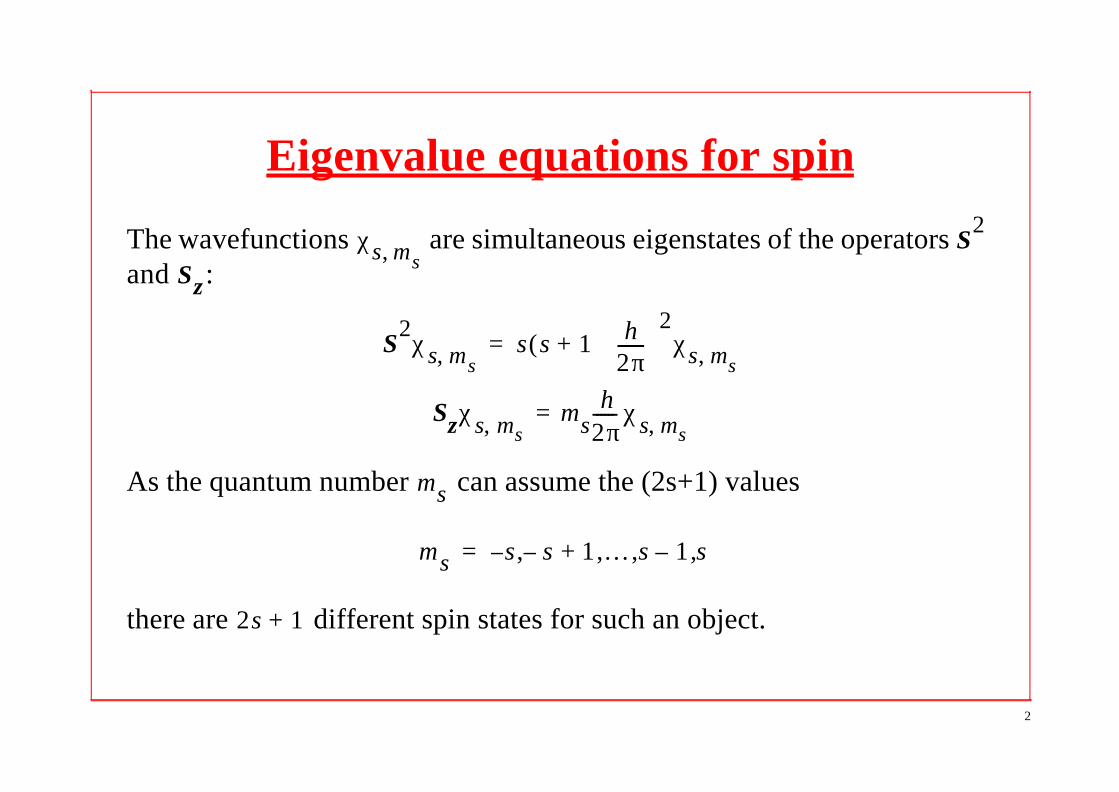
Eigenvalue equations for spin

The wavefunctions are simultaneous eigenstates of the operators and :

As the quantum number can assume the (2s+1) values

there are different spin states for such an object.

χs ms, S2

Sz

S2χs ms, s s 1+( ) h

2π------

2χs ms,=

Szχs ms, msh

2π------ χs ms,=

ms

ms s s– 1+ … s 1– s,,,,–=

2s 1+

3

Spin space

For each value of the quantum number , there is

a spin space of (2s+1) dimensions

for which the eigenfunctions form a basis.

Any spin wavefunction (with the same value) can be written as a super-position of the states .

= unit basis vectors of the (2s+1)-dimensional spin space

(compare with , the unit basis vectors of ordinary space)

s

χs ms,

sχs ms,

χs ms,

ux uy uz, ,

4

States of spin 1/2

The spin eigenfunctions for a particle with spin 1/2 are denoted by

where the first function describes the spin state with and the sec-ond function describes the spin state with .

These two functions are the basis in a two-dimensional spin space. Any function (‘vector’) in that space can be written as

where the constants and can be thought of as the ‘coordinates’ of the ‘vector’ in the two-dimensional spin space.

χs ms,χ1

2--- 1

2---,

χ12---

12---–,

,

ms 1 2⁄=ms 1– 2⁄=

χ12---

c1χ12--- 1

2---,

c2χ12---

12---–,

+=

c1 c2

5

The matrix representation

The operators , , and are represented by the (2s+1)x(2s+1) ma-trices

The simultaneous eigenfunctions of the operators and are given by the column vectors and

S2

Sx Sy Sz

Sxh

4π------ 0 1

1 0

= Syh

4π------ 0 i–

i 0

=

Szh

4π------ 1 0

0 1–

= S2 3h

2

16π2

------------ 1 0

0 1

=

S2

Sz

χ12--- 1

2---,

1

0

= χ12---

12---–,

0

1

=

6

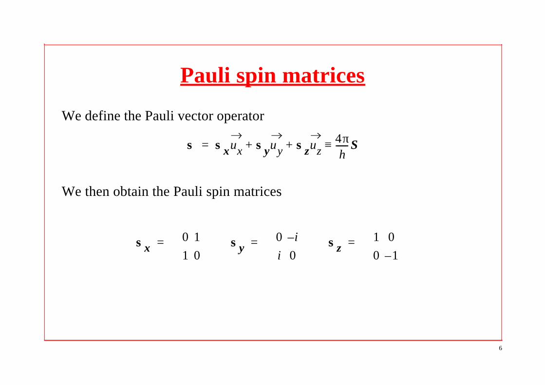
Pauli spin matrices

We define the Pauli vector operator

We then obtain the Pauli spin matrices

σ σxux σyuy σzuz+ + 4πh

------ S≡=

σx0 1

1 0

= σy0 i–

i 0

= σz1 0

0 1–

=

RAF211 - CZJ 1

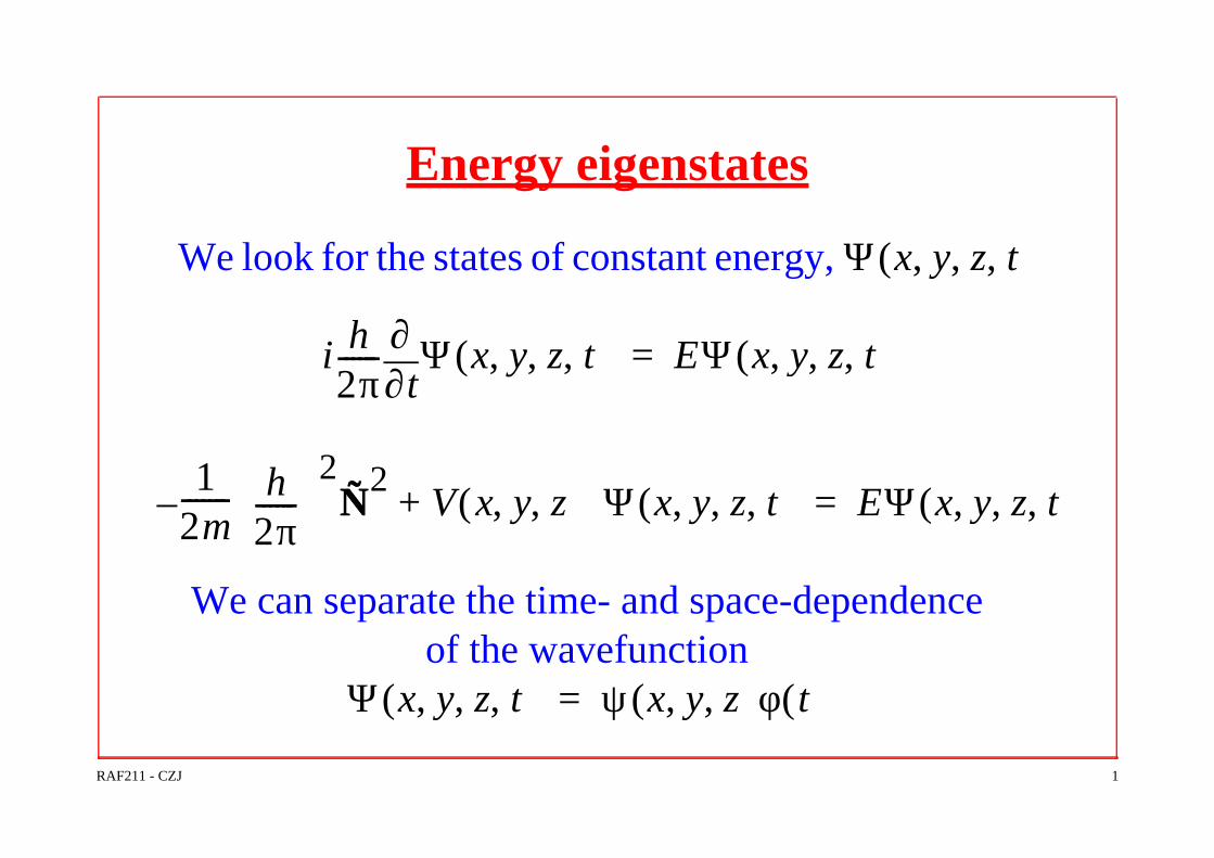
Energy eigenstates

We look for the states of constant energy,

We can separate the time- and space-dependence of the wavefunction

Ψ x y z t, , ,( )

i h2π------

t∂∂ Ψ x y z t, , ,( ) EΨ x y z t, , ,( )=

12m-------– h

2π------

2∇∇2

V x y z, ,( )+ Ψ x y z t, , ,( ) EΨ x y z t, , ,( )=

Ψ x y z t, , ,( ) ψ x y z, ,( )φ t( )=

RAF211 - CZJ 2

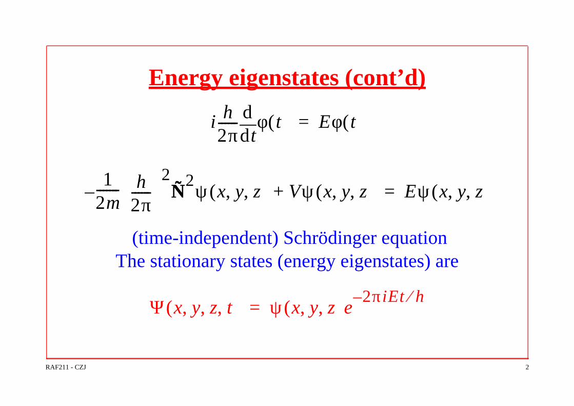
Energy eigenstates (cont’d)

(time-independent) Schrödinger equationThe stationary states (energy eigenstates) are

i h2π------

tdd φ t( ) Eφ t( )=

12m-------– h

2π------

2∇∇2ψ x y z, ,( ) V+ ψ x y z, ,( ) Eψ x y z, ,( )=

Ψ x y z t, , ,( ) ψ x y z, ,( )e2πiEt h⁄–

=

RAF211 - CZJ 3

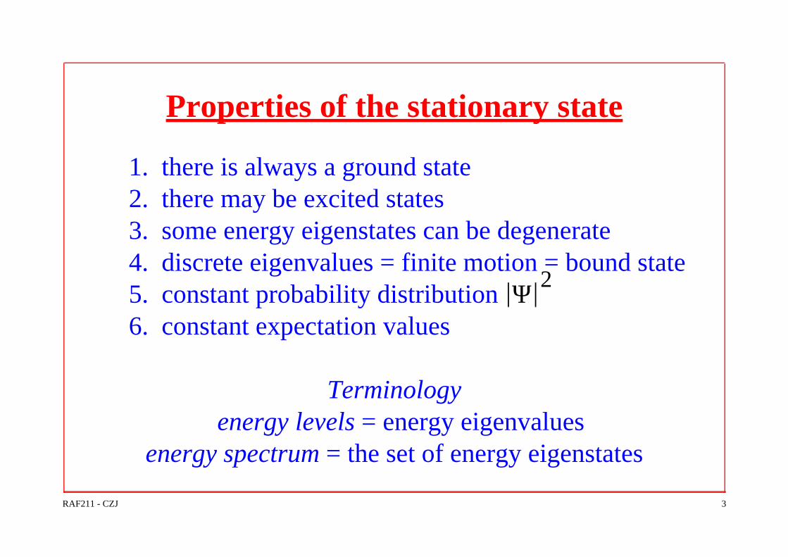
Properties of the stationary state

1. there is always a ground state 2. there may be excited states3. some energy eigenstates can be degenerate4. discrete eigenvalues = finite motion = bound state5. constant probability distribution 6. constant expectation values

Terminology energy levels = energy eigenvalues

energy spectrum = the set of energy eigenstates

Ψ 2

RAF211 - CZJ 4

Application: The free particle

We want to find the stationary states of a particlesthat moves in the x-direction, V=0, E=K

The Schrödinger equation

has the solution:

where

12m-------– h

2π------

2

x2

2

d

d ψ Eψ=

ψ x( ) c1eikx

c2ei– kx

+=

k 2π 2mE h⁄=

RAF211 - CZJ 5

Application: The free particle (cont’d)

We include the time-dependence

non-relativistic motion:

Combining with , we obtain

Ψ x t,( ) c1eikx

c2ei– kx

+( )e2πiEt h⁄–

=

E p2

2m( )⁄=

k 2π 2mE h⁄=

Ψ x t,( ) c1e2πipx h⁄

c2e2πipx h⁄–

+( )e2πiEt h⁄–

=

RAF211 - CZJ 6

Interpretation of free particle wavefunction

1. superposition of a particle’s momentum eigenstatesindeterminate: direction of motion, position

degenerate energy eigenvalues

2. superposition of two plane waves

and

of angular frequency and wavelength

E p2

2m( )⁄=

Ψ1 x t,( ) c1eikx

eiωt–

= Ψ2 x t,( ) c2ei– kx

eiωt–

=

ω 2πf 2πE h⁄ E⇒ hf= = =λ 2π k⁄ λ h p⁄=⇒=

RAF211 - CZJ 7

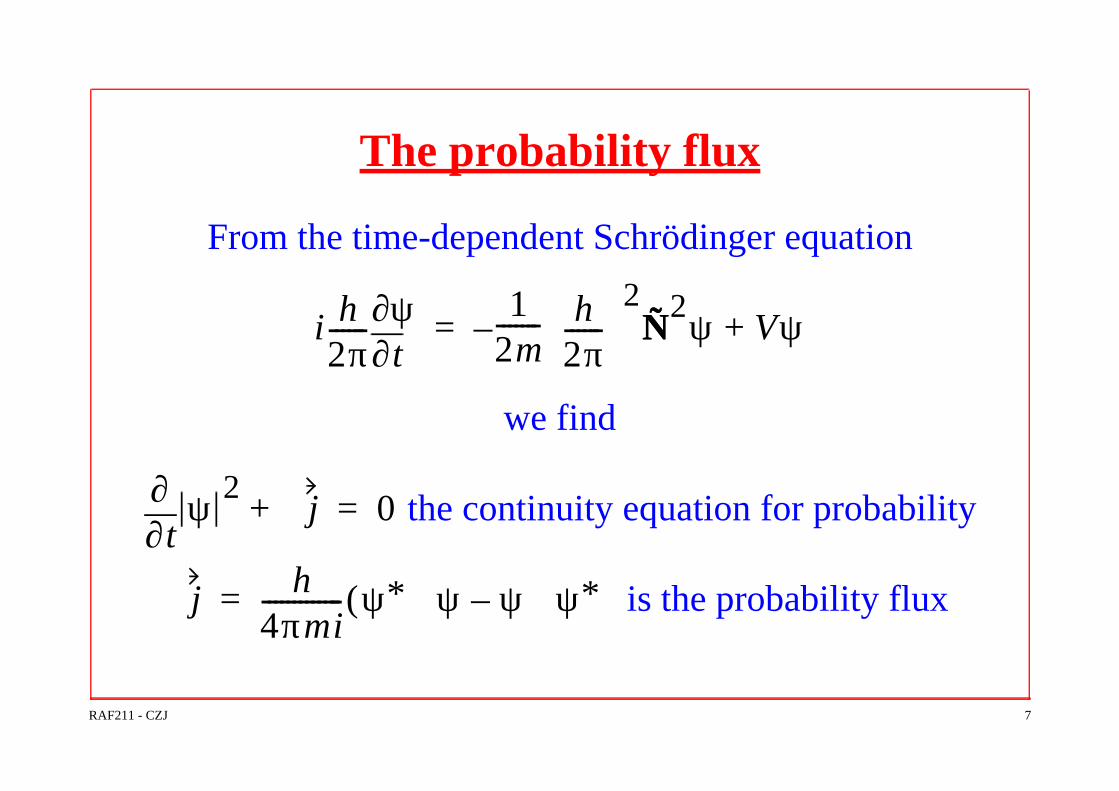
The probability flux

From the time-dependent Schrödinger equation

we find

the continuity equation for probability

is the probability flux

i h2π------

t∂∂ψ 1

2m-------– h

2π------

2∇∇2ψ V+ ψ=

t∂∂ ψ 2 ∇j+ 0=

j h4πmi------------- ψ∗∇ψ ψ∇ψ∗–( )=

RAF211 - CZJ 8

Properties of the Schrödinger equation

1. is single-valued

2. and are continuous

3. objects cannot penetrate regions of infinite potential

4. only negative potentials that vanish at infinity can give bound states (application: Coulomb potential)

ψ

ψ dψ dx⁄

RAF211 - CZJ 9

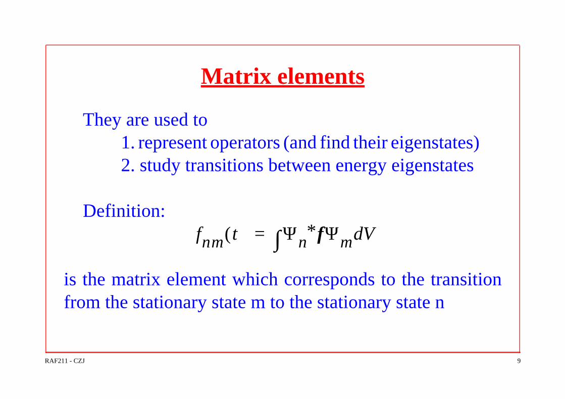
Matrix elements

They are used to1. represent operators (and find their eigenstates) 2. study transitions between energy eigenstates

Definition:

is the matrix element which corresponds to the transitionfrom the stationary state m to the stationary state n

fnm t( ) Ψn∗fΨm Vd∫=

RAF211 - CZJ 10

Transitions

Why do we study transitions?

Because that’s when radiation is produced

How about ?∆E ∆t h 4π( )⁄=⋅

RAF211 - CZJ 11

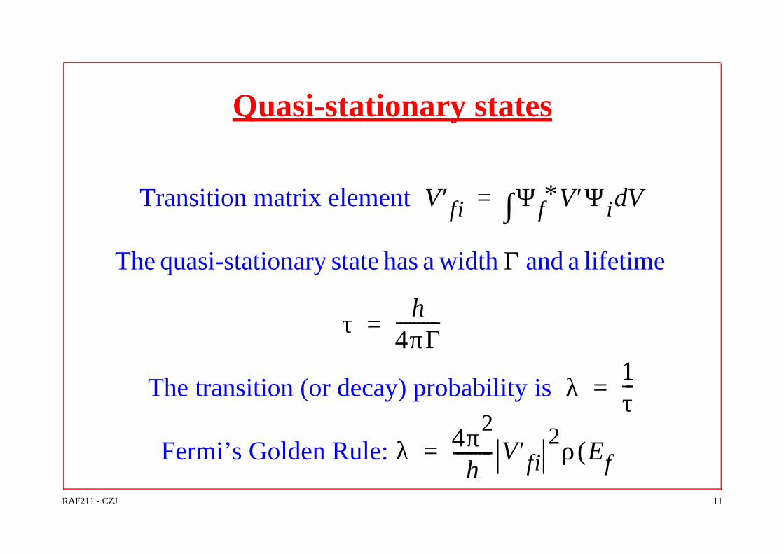
Quasi-stationary states

Transition matrix element

The quasi-stationary state has a width and a lifetime

The transition (or decay) probability is

Fermi’s Golden Rule:

V′fi Ψf∗V′Ψi Vd∫=

Γ

τh

4πΓ----------=

λ1τ---=

λ 4π2

h--------- V′fi

2ρ Ef( )=

RAF211 - CZJ 1

The atom

a Stationary states for central potentialsa Solutions for the hydrogen atoma Magnetic dipole moment of hydrogena The independent electron modela Ground state of atomsa The Zeeman effecta Spin-orbit couplinga (X-rays and Auger electrons)a (Fluorescence)

RAF211 - CZJ 2

Spherically symmetric potentials

We will look for stationary states describing the 3d motion of an object in a central potential V(r)

r We will not consider the time dependence of the wavefunctions (measurements)

Our stationary states will be used to describe the electron states of the hydrogen atom.

They are also eigenstates of and .L2

Lz

RAF211 - CZJ 3

The Schrödinger equation

Stationary states:

but we already have the spherical harmonicsso we can write and solve the radial equation:

ψ r φ θ, ,( )

12m-------– h

2π------

2

r2

2

∂

∂ 2r---

r∂∂+ ψ 1

2m------- 1

r2

-----L2ψ V r( )+ + ψ Eψ=

ψ r φ θ, ,( ) R r( )Ylm θ φ,( )=

12m-------– h

2π------

2

r2

2

d

d 2r---

rdd+

1

r2

-----– l l 1+( ) V r( )+

R r( ) ER r( )=

RAF211 - CZJ 4

Application: the hydrogen atom

r = distance between the electron and the protonThe radial equation can be use for provided

that

VH r( )e

2

4πε0------------– 1

r---=

VH r( )

m µmpme

mp me+--------------------=→

RAF211 - CZJ 5

The solution

RAF211 - CZJ 6

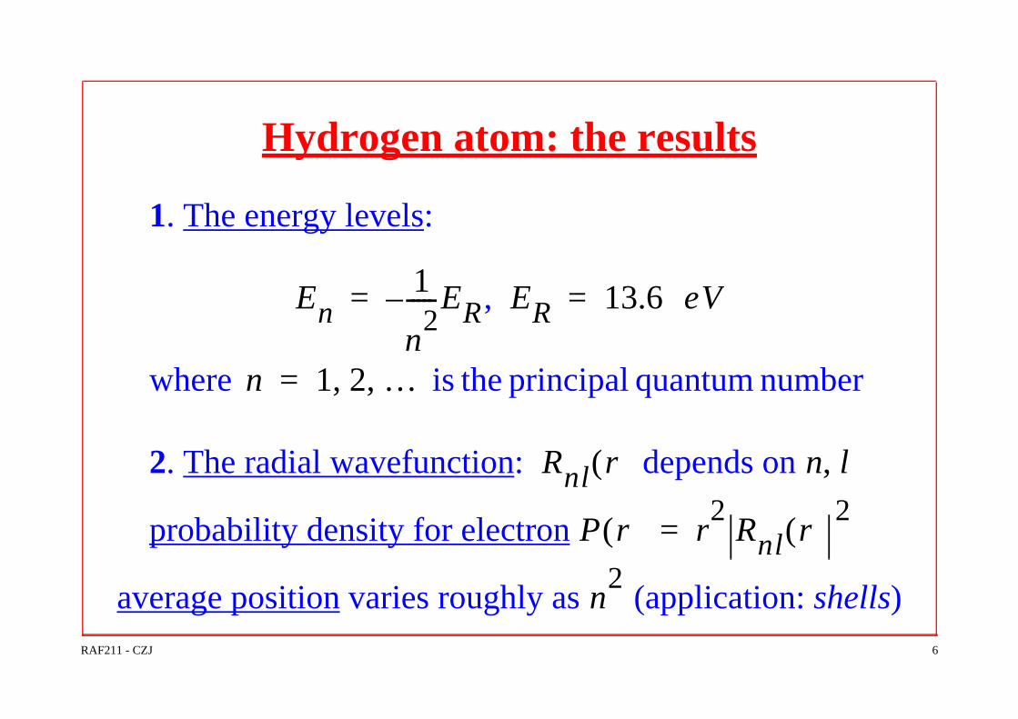
Hydrogen atom: the results

1. The energy levels:

,

where is the principal quantum number

2. The radial wavefunction: depends on

probability density for electron

average position varies roughly as (application: shells)

En1

n2

-----ER–= ER 13.6 eV=

n 1 2 …, ,=

Rnl r( ) n l,

P r( ) r2

Rnl r( ) 2=

n2

RAF211 - CZJ 7

Hydrogen atom : the results (cont’d)

3. The spatial dependence of the wavefunction: but

4. The parity of hydrogen:

5. ‘Orbitals’ instead of ‘orbits’

6. Spin: the complete wavefunction is

7. Degeneracy of energy levels:

ψnlm r φ θ, ,( ) Rnl r( )Ylm

θ φ,( )= ψnl r θ,( ) 2

Pψnlm 1–( )lψnlm=

ψnlmlms

2n2

RAF211 - CZJ 8

Magnetic dipole moment of hydrogen

In general, is due to angular momentum

The hydrogen atom has: (a) orbital angular momentum, (b) spin orbital momentum,

We thus have ‘two’ magnetic dipole moments:

and

µ

ls

µL z,eh

4πme--------------ml– mlµB–= = µS z,

eh2πme--------------ms– 2msµB–= =

RAF211 - CZJ 9

The independent electron model

We describe many-electron atoms by using an ‘effective potential’ in the Schrödinger equation

- wavefunction: as in hydrogen atom but

- energy levels: depend on = 0, 1, 2, 3, ...name of the level: s, p, d, f, ...

- notation for electronic energy levels: nl, e.g. 1s- energy ordering: 1s, 2s, 2p, 3s, 3p, 4s, 3d, 4p, 5s, ...

ψnlmlms

n l,l

RAF211 - CZJ 10

The independent electron model

Energy levels

s and p orbitals ‘go’ closer to the nucleus

E

1s

2s2p

3s3p4s 3d4p

5s 4d5p

RAF211 - CZJ 11

Application of the independent electron model

RAF211 - CZJ 12

The Pauli principle

‘For each set of values for the quantum numbers , we can have only one electron’n l ml ms, , ,

RAF211 - CZJ 13

Applications of the model (i.e.m)

- electronic structure of atoms- determine the chemical and electromagnetic

properties of the atom- calculate angular momentum of atom (L-S coupling)

- explain optical transitions- ground state for light atoms

r cannot be used for the study of X-rays (heavy atoms)

RAF211 - CZJ 14

(Optical) transitions

frequency of emitted/absorbed photon:

selection rule:

ν 1h--- Ei Ef–( )=

∆l 1±=

RAF211 - CZJ 15

The ground state of atoms

Hund’s rules

1. add spins of valence electrons so that the total spin is maximized

2. add the orbital angular momenta of valence electrons so that is max.

3. and are added to calculate

Lz mlh

2π------

∑ h2π------

mL= =

S J J

RAF211 - CZJ 16

The Zeeman effect

Assume ‘spinless’ valence electron with n=2, l=1 in a magnetic field (along z-axis)

Interaction energy between the magnetic moment and the magnetic field: U µL z, B– mlµBB= =

field off field on

E22E + µBB

E2µB B-

RAF211 - CZJ 17

Spin-orbit coupling

The nucleus produces a magnetic field thatinteracts with the spin magnetic dipole

moment of the electron

Electron states: eigenstates of (i.e.m.)

notation:

U µS z, B– 2msµBB µBB±= = =

J2

L2

S2

Jz, , ,

A2s 1+

j

300303 - CZJ 1

The nucleus

The Geiger-Marsden experiment (1909)Scattering of a particles by gold and silver foils showed that someof the particles were backscattered. The observed scattering angles could only be explained by a charge ‘concentrated’ over arange of a few times 10-14 m.

Atoms are ‘empty’!With an atom occuping a room of sides of 10 m, the nucleuswould hardly stretch across 1 mm. The nucleus carries about99.95% of the atomic mass and has an extremely high density, ofthe order of 1014 times the density of water.

300303 - CZJ 2

The forces in the nucleus

There are two types of interaction acting in the nucleus:a strong interaction: attractive force between nucleons. It behavessimilarly for neutrons and protons because of their quark composi-tion (udd and uud)an electromagnetic interaction: repulsive force between protons

By ‘nuclear forces’ we denote the first type. They hold the nucleus together, which also explains the size of the nuclei.

The theory of strong interactions (QCD) can only be solved analytically for quarks and gluons which are not confined in hadronsbecause of the magnitude of the coupling constant of the strong interactions. Therefore, we only have models to describe the potential in the nucleus.

300303 - CZJ 3

The mass of the nucleus

A nucleus with N neutrons and Z protons has a mass equal to

B is the binding energy of the nucleus, i.e. the energy required tobreak up the nucleus to its constituents. B is always positive because the nucleus is a bound system.

Typical value for B: 8 MeV per nucleon. The most tightly boundnucleus is 62Ni with B=8.795 MeV per nucleon

Compare B with the mass of a nucleon: ~1000 MeVand atomic energies, i.e. the binding energy of H: ~14 eV

mA Nmn Zmp B c2

⁄–+=

300303 - CZJ 4

Calculating binding energy

is the binding energy of the electrons in the atom (at least 4 ordersof magnitude smaller than the mass of the nucleus). The binding energy of the nucleus, , is

The calculation is done using atomic masses, .

matomc2

mnucleusc2

Zmelectronc2

Belectron+ +=

Belectron

B Zmpc2

Nmnc2

mnucleusc2

–+=

B Zmpc2

Zmec2

+( ) Nmnc2

mnucleusc2

Zmec2

+( )–+=

B ZmH

11 0

c2

Nmnc2

matomc2

–+=

c2

931 MeV u⁄=

300303 - CZJ 5

Separation energy

Neutron (proton) separation energy is the energy required to remove a neutron (proton) from a nucleus and is equal to the difference of the binding energies of the two nuclei:

Separation energies in nuclear physics are analogous to ionization energies in atomic physics: they refer to the binding of the outermost nucleon. Separation energies also show shell structure in the nucleuslike ionization energies show shell structure in the atom.

Sn B XAZ N( ) B X

A 1–Z N 1–( )–=

Sp B XAZ N( ) B X

A 1–Z 1– N( )–=

300303 - CZJ 6

Binding energy per nucleon

A<62: light nucleus + light nucleus heavy nucleus (fusion)A>62: heavy nucleus light nucleus + light nucleus (fission)

→→

300303 - CZJ 7

Mass distribution and nuclear radius

From electron scattering experi-ments, we know that the protonsare distributed in the nucleus asthese curves show.

The distance at which the curvehas half of its central value isdefined as the radius, R, of the nucleus.

Neutron distributions are similar. distance from centre of the nucleus (fm)

dens

ity (

nucl

eons

/fm

3 )R r0A

1 3⁄r0 1.07 fm≈,≈

300303 - CZJ 8

‘Spin’ and parity

Protons and neutrons move inside the nucleons, so they have bothintrinsic angular momentum and orbital angular momentum. The total angular momentum of the nucleus, J, is calculated using J-J coupling on the momenta of the nucleons.

J is usually called the spin of the nucleus!

The total orbital angular momentum, l, of the nucleus, determinesthe parity, λ, of the nucleus (under space reflection):

In decay diagrams, the nuclei are denoted by , i.e. or .

λ 1–( )l=

Jλ

J+ J

-

300303 - CZJ 9

Multipole moments

A nucleus is a distribution of charges and currents, which produceelectric and magnetic fields. The space-dependence of these fieldsis described in terms of the ‘multipole moments’ of the nucleus.They are labeled by their order, L:

• L=0 (0th or monopole moment): the electric field varies as r-2

• L=1 (1st or dipole moment): the electric field varies as r-3

• L=2 (2nd or quadrupole moment): the electric field varies as r-4

• ...We have the same moments for the magnetic field (no monopole).

The moments of the nucleus reflect its shape: a spherical nucleus hasonly a monopole electric moment.

300303 - CZJ 10

The parity of the moments

The multipole moments of the nucleus are quantum mechanicallydescribed by operators, which are functions of the coordinates x, y,and z, and therefore have a parity eigenvalue.

The parity of electric multipole moments is (-1)L

The parity of electric multipole moments is (-1)L+1

(L=order of the moment)

Only even-parity moments exist: electric monopole, magnetic dipole, electric quadrupole, etc.

(Krane, ‘Introductory nuclear physics’, §3.5)

300303 - CZJ 11

Excited states

The nucleus, being a bound quantum mechanical system, can haveexcited states, like atoms have. The density of excited states increas-es as the excitation energy does. Excited states are reached as a resultof a nuclear reaction.

Examples:1. Single-particle states: excited states of nuclei with filled shells + one valence nucleon that can be excited without disturbing the ‘core’.2. Rotational collective states: nuclei sufficiently deformed from the spherical shape have excited states that are described by a rotational motion of the entire nucleus.3. Vibrational collective states: visualized as harmonic oscillations in shape about a spherical mean.

300303 - CZJ 12

Example of single-particle excited states:

300303 - CZJ 13

Example of rotational and vibrational nuclei:

300303 - CZJ 14

Times and relativity

Typical kinetic energy of a nucleon within a nucleus: 30 MeV. This givesa velocity ~ 107 m/s and for a nuclear circumference of 10 fm, the nucleonwould make a complete orbit in ~ 10-22 s.

This is the characteristic time for nucleon motions in the nucleus. (compare with the time it takes an electron to complete one orbit and which is of the order 10-16 s.)

Considering the typical nucleon kinetic energy above (30 MeV), we con-clude that the motion of the nucleons is non-relativistic.Most nuclear phenomena can be described by non-relativistic quantum me-chanics. Exceptions: (a) beta decay, where the electron and neutrino mustbe described relativistically using Dirac’s equation, (b) nuclear scatteringwith projectile energies of several hundred MeV per nucleon require a rel-ativistic description of the kinematics of the collision.