
What is a Photon? Foundations of Quantum Field Theory than one photon appears/disappears. In the...
105
What is a Photon? Foundations of Quantum Field Theory C. G. Torre May 4, 2018
Transcript of What is a Photon? Foundations of Quantum Field Theory than one photon appears/disappears. In the...

What is a Photon?
Foundations of Quantum Field Theory
C. G. Torre
May 4, 2018

2
What is a Photon?Foundations of Quantum Field Theory
Version 1.0
Copyright c© 2018. Charles Torre, Utah State University.
PDF created May 4, 2018

Contents
1 Introduction 51.1 Why do we need this course? . . . . . . . . . . . . . . . . . . . . . . . . . . . . . . . 51.2 Why do we need quantum fields? . . . . . . . . . . . . . . . . . . . . . . . . . . . . . 51.3 Problems . . . . . . . . . . . . . . . . . . . . . . . . . . . . . . . . . . . . . . . . . . 6
2 The Harmonic Oscillator 72.1 Classical mechanics: Lagrangian, Hamiltonian, and equations of motion . . . . . . . 72.2 Classical mechanics: coupled oscillations . . . . . . . . . . . . . . . . . . . . . . . . . 82.3 The postulates of quantum mechanics . . . . . . . . . . . . . . . . . . . . . . . . . . 102.4 The quantum oscillator . . . . . . . . . . . . . . . . . . . . . . . . . . . . . . . . . . 112.5 Energy spectrum . . . . . . . . . . . . . . . . . . . . . . . . . . . . . . . . . . . . . . 122.6 Position, momentum, and their continuous spectra . . . . . . . . . . . . . . . . . . . 15
2.6.1 Position . . . . . . . . . . . . . . . . . . . . . . . . . . . . . . . . . . . . . . . 152.6.2 Momentum . . . . . . . . . . . . . . . . . . . . . . . . . . . . . . . . . . . . . 172.6.3 General formalism . . . . . . . . . . . . . . . . . . . . . . . . . . . . . . . . . 19
2.7 Time evolution . . . . . . . . . . . . . . . . . . . . . . . . . . . . . . . . . . . . . . . 202.8 Coherent States . . . . . . . . . . . . . . . . . . . . . . . . . . . . . . . . . . . . . . . 222.9 Problems . . . . . . . . . . . . . . . . . . . . . . . . . . . . . . . . . . . . . . . . . . 23
3 Tensor Products and Identical Particles 273.1 Definition of the tensor product . . . . . . . . . . . . . . . . . . . . . . . . . . . . . . 273.2 Observables and the tensor product . . . . . . . . . . . . . . . . . . . . . . . . . . . . 303.3 Symmetric and antisymmetric tensors. Identical particles. . . . . . . . . . . . . . . . 323.4 Symmetrization and anti-symmetrization for any number of particles . . . . . . . . . 343.5 Problems . . . . . . . . . . . . . . . . . . . . . . . . . . . . . . . . . . . . . . . . . . 35
4 Fock Space 384.1 Definitions . . . . . . . . . . . . . . . . . . . . . . . . . . . . . . . . . . . . . . . . . . 384.2 Occupation numbers. Creation and annihilation operators. . . . . . . . . . . . . . . . 404.3 Observables. Field operators. . . . . . . . . . . . . . . . . . . . . . . . . . . . . . . . 43
4.3.1 1-particle observables . . . . . . . . . . . . . . . . . . . . . . . . . . . . . . . 434.3.2 2-particle observables . . . . . . . . . . . . . . . . . . . . . . . . . . . . . . . 464.3.3 Field operators and wave functions . . . . . . . . . . . . . . . . . . . . . . . . 46
4.4 Time evolution of the field operators . . . . . . . . . . . . . . . . . . . . . . . . . . . 484.5 General formalism . . . . . . . . . . . . . . . . . . . . . . . . . . . . . . . . . . . . . 50
3

4 CONTENTS
4.6 Relation to the Hilbert space of quantum normal modes . . . . . . . . . . . . . . . . 534.7 Problems . . . . . . . . . . . . . . . . . . . . . . . . . . . . . . . . . . . . . . . . . . 53
5 Electromagnetic Fields 565.1 Maxwell equations . . . . . . . . . . . . . . . . . . . . . . . . . . . . . . . . . . . . . 56
5.1.1 The basic structure of the Maxwell equations . . . . . . . . . . . . . . . . . . 575.1.2 Continuity equation and conservation of electric charge . . . . . . . . . . . . 58
5.2 The electromagnetic wave equation . . . . . . . . . . . . . . . . . . . . . . . . . . . . 595.3 Electromagnetic energy, momentum, and angular momentum . . . . . . . . . . . . . 62
5.3.1 Energy . . . . . . . . . . . . . . . . . . . . . . . . . . . . . . . . . . . . . . . . 625.3.2 Momentum and angular momentum . . . . . . . . . . . . . . . . . . . . . . . 64
5.4 Electromagnetic potentials . . . . . . . . . . . . . . . . . . . . . . . . . . . . . . . . . 655.5 Role of the sources . . . . . . . . . . . . . . . . . . . . . . . . . . . . . . . . . . . . . 675.6 Solution to the source-free Maxwell equations . . . . . . . . . . . . . . . . . . . . . . 685.7 Energy and momentum, revisited . . . . . . . . . . . . . . . . . . . . . . . . . . . . . 695.8 Angular momentum, revisited . . . . . . . . . . . . . . . . . . . . . . . . . . . . . . . 715.9 Periodic boundary conditions . . . . . . . . . . . . . . . . . . . . . . . . . . . . . . . 725.10 Motion of a charged particle in an electromagnetic field . . . . . . . . . . . . . . . . 735.11 Problems . . . . . . . . . . . . . . . . . . . . . . . . . . . . . . . . . . . . . . . . . . 74
6 What is a Photon? 776.1 Hilbert space for the electromagnetic field . . . . . . . . . . . . . . . . . . . . . . . . 776.2 The Hamiltonian. Stationary states . . . . . . . . . . . . . . . . . . . . . . . . . . . . 786.3 Momentum and Helicity . . . . . . . . . . . . . . . . . . . . . . . . . . . . . . . . . . 796.4 Interpretation in terms of photons . . . . . . . . . . . . . . . . . . . . . . . . . . . . 806.5 Time evolution . . . . . . . . . . . . . . . . . . . . . . . . . . . . . . . . . . . . . . . 826.6 The electromagnetic field operator . . . . . . . . . . . . . . . . . . . . . . . . . . . . 826.7 Vacuum fluctuations . . . . . . . . . . . . . . . . . . . . . . . . . . . . . . . . . . . . 836.8 Coherent states . . . . . . . . . . . . . . . . . . . . . . . . . . . . . . . . . . . . . . . 856.9 Photon interference . . . . . . . . . . . . . . . . . . . . . . . . . . . . . . . . . . . . . 866.10 Limitations on the particle interpretation . . . . . . . . . . . . . . . . . . . . . . . . 886.11 Problems . . . . . . . . . . . . . . . . . . . . . . . . . . . . . . . . . . . . . . . . . . 89
7 Spontaneous Emission 917.1 Hydrogenic atoms . . . . . . . . . . . . . . . . . . . . . . . . . . . . . . . . . . . . . 917.2 The hydrogenic atom coupled to photons . . . . . . . . . . . . . . . . . . . . . . . . 927.3 Perturbation theory. Fermi’s Golden Rule . . . . . . . . . . . . . . . . . . . . . . . . 947.4 Spontaneous emission . . . . . . . . . . . . . . . . . . . . . . . . . . . . . . . . . . . 96
7.4.1 First-order approximation . . . . . . . . . . . . . . . . . . . . . . . . . . . . . 967.4.2 Electric dipole transitions . . . . . . . . . . . . . . . . . . . . . . . . . . . . . 987.4.3 Lifetime of 2P → 1S . . . . . . . . . . . . . . . . . . . . . . . . . . . . . . . . 100
7.5 Another perspective . . . . . . . . . . . . . . . . . . . . . . . . . . . . . . . . . . . . 1017.6 Problems . . . . . . . . . . . . . . . . . . . . . . . . . . . . . . . . . . . . . . . . . . 102
8 Epilogue 103
Bibliography 105
Chapter 1
Introduction
This is a brief, informal, and relatively low-level course on the foundations of quantum field theory.The prerequisites are undergraduate courses in quantum mechanics and electromagnetism.
1.1 Why do we need this course?
I have always been dismayed by the fact that one can get a PhD in physics yet never be exposed tothe theory of the photon. To be sure, we talk about photons all the time and we know some of theirsalient properties. But how do they arise in the framework of quantum theory? What do they haveto do with the more familiar theory of electromagnetism? Of course, most people don’t ever learnwhat a photon really is because a photon is an entity which arises in quantum field theory, which isnot a physics class most people get to take. Quantum field theory typically arises in most physicscurricula either in an advanced quantum mechanics course where one wants to do some many bodytheory, in a course on quantum optics, or in a course meant to explain the theory underlying highenergy particle physics. Of course these subjects can be a bit daunting for someone who just wantsto know what it is they are talking about when they use the term “photon”. But the theory ofthe photon is not that complicated. The new ingredients needed to understand the theoreticaldescription of the photon can be explained in some detail to anyone who has assimilated courses inquantum mechanics and electrodynamics. The principal goal of this course is really just to explainwhat are the main ideas behind the quantum field – this quantum “stuff” out of which everythingis made. Constructing the quantum field in the context of electromagnetism leads immediately tothe notion of the photon.
1.2 Why do we need quantum fields?
Let me remind you of the phenomenon of spontaneous emission, in which an atomic electron in anexcited state will spontaneously emit one (or more) photons and end up in a lower energy state. Thisphenomenon will take place in the absence of any external stimulus and cannot be explained usingthe usual quantum mechanical model of the atom. Indeed, the usual quantum mechanical modelof atomic energy levels represents them as stationary states. If an atomic electron occupying anatomic energy level were truly in a stationary state there could never be any spontaneous emission
5
6 CHAPTER 1. INTRODUCTION
since a stationary state has no time dependent behavior. The only way out of this conundrum isto suppose that atomic energy levels are not really stationary states once you take into account theinteraction of photons and electrons. So now we need a quantum theory of more than one particle.We know how to do this, of course. But there is a wrinkle. Think again about the emission of aphoton by an atomic electron. The initial state of the system has an electron. The final state of thesystem has an electron and a photon. Moreover, it is possible to have atomic transitions in whichmore than one photon appears/disappears. In the usual quantum mechanical formalism the numberof particles is fixed. Indeed, the normalization of the wave function for a particle (or for particles)can be viewed as saying that the particle (or particles) is (or are) always somewhere. Clearly wewill not be able to describe such processes using the standard quantum mechanical models. If thisisn’t enough, I remind you that there exist situations in which a photon may disappear, producingan electron-positron pair and, conversely, in which an electron-positron can turn into a photon. Soeven electrons and positrons are not immune from the appearance/disappearance phenomena.
Remarkably, it is possible to understand these variable-particle processes using the axioms ofquantum theory, provided these axioms are used in a clever enough way. This new and improveduse of quantum mechanics is usually called quantum field theory since it can be viewed as anapplication of the basic axioms of quantum mechanics to continuous systems (field theories) ratherthan mechanical systems. The picture that emerges is that the building blocks of matter andits interactions consist of neither particles nor waves, but a new kind of entity: a quantum field.Quantum mechanical particles and their wave-particle duality then become particularly simplemanifestations of the quantum field. Every type of elementary particle is described by a quantumfield (although the groupings by type depend upon the sophistication of the model). There is anelectron field, a photon field, a neutrino field, a quark field and so forth.1
Quantum field theory (QFT) has led to spectacular successes in describing the behavior of awide variety of atomic and subatomic phenomena. The success is not just qualitative; some ofthe most precise measurements known involve minute properties of the spectra of atoms. Theseproperties are predicted via quantum field theory and, so far, the agreement with experiment isperfect.
Here I will give a brief, superficial introduction to some of the fundamental ideas underlyingQFT. My principal goal will be just to show how QFT is used to describe photons and spontaneousemission. My strategy is to echo Dirac’s original constructions, presented in a very influentialmonograph in 1930 [1], which was aimed at doing just this, and eventually led to modern quantumfield theory. In doing so I have borrowed from Merzbacher’s [2] and Sakurai’s [3] treatment of someof these ideas, which are very clear and closely aligned with the concepts I want to introduce to you.It takes a bit more work to use these same ideas to describe, say, electrons in terms of quantumfields. Yet more work is needed to analyze the interaction of these particles (better: these fields).Quantum field theory is a very rich subject, still a subject of intense research.
1.3 Problems
1. What is the experimental value for the mean lifetime of the 2p state of hydrogen?
2. What is positronium? What is its mean lifetime?
1Relativistic fields include the anti-particles as well.
Chapter 2
The Harmonic Oscillator
The harmonic oscillator describes motion near stable equilibrium. Its quantum mechanical mani-festation is precisely what is needed to understand free (non-interacting) fields and their particleexcitations. So we must spend some time establishing the facts we will need concerning the quan-tum oscillator. This will also give me a chance to review with you the principal parts of quantummechanics that we will need to define quantum field theory.
2.1 Classical mechanics: Lagrangian, Hamiltonian, and equa-tions of motion
Before reviewing the quantum oscillator, it is good to first get oriented by reviewing its classicallimit. A harmonic oscillator is characterized by 2 parameters: its mass m and its angular frequencyω. The Lagrangian and Hamiltonian for a (classical) harmonic oscillator are given respectively by
L(x, x) =1
2mx2 − 1
2mω2x2, H(x, p) =
p2
2m+
1
2mω2x2. (2.1)
Here x is the displacement from equilibrium, x is the velocity, and p is the momentum canonicallyconjugate to x. The Euler-Lagrange equations are
∂L
∂x− d
dt
∂L
∂x= 0 ⇐⇒ x+ ω2x = 0. (2.2)
The Hamilton equations are
x =∂H
∂p, p = −∂H
∂x⇐⇒ x =
p
m, p = −mω2x. (2.3)
You can verify that the Lagrangian and Hamiltonian forms of the equations of motion are equivalent.The general solution to the equations of motion is given by
x(t) = A cos(ωt) +B sin(ωt), (2.4)
where
A = x(0), B =1
ωx(0). (2.5)
7

8 CHAPTER 2. THE HARMONIC OSCILLATOR
A very useful representation of the solutions to the oscillator equation involves complex amplitudes.Define
a =
√mω
2(x+
i
mωp), a∗ =
√mω
2(x− i
mωp). (2.6)
The variables a and a∗ are just as good for describing the motion as x and p. In particular thedisplacement comes from the real part of a and the momentum from the imaginary part of a. Interms of the complex amplitudes, the general solution to the equation of motion takes the verysimple form
a(t) = a(0)e−iωt, a∗(t) = a∗(0)eiωt. (2.7)
The Hamiltonian is also the energy of the oscillator. It is conserved, that is, unchanging in time:
H(t) =p(t)2
2m+
1
2mω2x(t)2 =
p(0)2
2m+
1
2mω2x(0)2 = H(0). (2.8)
In terms of the complex amplitudes this result is particularly simple:
H(t) = ωa∗(t)a(t) = ω(a∗(0)eiωt
) (a(0)e−iωt
)= ωa∗(0)a(0) = H(0). (2.9)
2.2 Classical mechanics: coupled oscillations
When a dynamical system has more than one degree of freedom, motion near stable equilibrium isin the form of coupled harmonic oscillations. Let us see how this happens.
Suppose the degrees of freedom are denoted by qi, i = 1, 2, . . . , n, and that the Lagrangian is ofthe form
L =1
2gij(q)q
iqj − V (q). (2.10)
I am using Einstein’s summation convention; there is a double sum in the first term of L. The“metric” gij(q) is an array which may depend upon the configuration coordinates. There is no lossof generality in assuming the metric to be symmetric,
gij = gji, (2.11)
since only the symmetric combination appears in the sum over i and j. The metric involves themasses and other parameters; it is often just a collection of constants, but need not be. The metricis also often diagonal (e.g., in spherical polar coordinates), but it need not be. The function Vrepresents the potential energy of interaction among the degrees of freedom of the system and withtheir environment.
Critical points of V , i.e., points qi0 such that(∂V
∂qi
)(q0) = 0, (2.12)
define equilibrium configurations of the system. We will suppose that the equilibrium is stable, i.e.,qi0 is a (local) minimum of V . Let us approximate the motion in the neighborhood of a point ofequilibrium by defining
yi = qi − qi0, (2.13)
2.2. CLASSICAL MECHANICS: COUPLED OSCILLATIONS 9
and expanding the Lagrangian in a Taylor series about yi = 0. To the first non-trivial order we get
L ≈ 1
2Mij y
iyj − 1
2Kijy
iyj ≡ L2 (2.14)
where
Mij = gij(q0), Kij =
(∂2V
∂qi∂qj
)(q0), (2.15)
and I have dropped an irrelevant additive constant V (q0), i.e., the zero point of potential energy hasbeen chosen to be at the equilibrium of interest, qi = qi0. The array of constants M is symmetric,Mij = Mji, and we assume that the potential energy is sufficiently smooth so that the matrix K ofsecond partial derivatives is symmetric at the critical point q0:
Kij = Kji. (2.16)
In this approximation, the Euler-Lagrange equations are
Mij yj +Kijy
j = 0, (2.17)
which are a coupled system of n homogeneous, linear ODEs with constant coefficients. Defining ~yas a column vector with entries yi, and viewing Mij and Kij as symmetric matrices M and K, wecan write the EL equations in the matrix form:
M~y = −K~y. (2.18)
Let us note that if qi0 is a point of stable equilibrium then the symmetric matrix K is non-negative, that is, it can have only non-negative eigenvalues.1 This is because a negative eigenvaluewill correspond to displacements yi which lower the potential energy in an arbitrarily small neigh-borhood of the equilibrium point, which contradicts our assumption of stable equilibrium. If theeigenvalues are positive then the point qi0 is a local minimum. All this means that qi0 is a point ofstable equilibrium if the quadratic form
K(~y) := Kijyiyj (2.19)
is positive, that is, K(~y) > 0 for all ~y 6= 0. Physically this means that any displacement yi fromequilibrium will increase the potential energy. All this discussion is just restating standard resultsfrom multivariate calculus.
Likewise, positivity of the kinetic energy implies that the symmetric matrix M should be positivedefinite. This means the quadratic form
M(~v) := Mijvivj (2.20)
is positive definite, i.e., M(~v) > 0 for all ~v 6= 0.I now would like to appeal to a nice result from linear algebra. For any K, if the quadratic form
defined by M is positive definite, then there exists a linear change of coordinates yi → xi:
xi = Λijyj , xi = Λij yj , (2.21)
1Note that a symmetric, real matrix always admits complete set of eigenvectors with real eigenvalues.

10 CHAPTER 2. THE HARMONIC OSCILLATOR
with inverseyi = (Λ−1)ijx
j , yi = (Λ−1)ij xj . (2.22)
such that in the new coordinates xi the approximate Lagrangian takes the form
L2 =1
2(x21 + x22 + · · ·+ x2n)− 1
2(ω2
1x21 + ω2
2x22 + · · ·+ ω2
nx2n), (2.23)
where ωi, i = 1, 2, . . . , n, are constants. In general these constants can be real, pure imaginary,or zero, depending on whether the eigenvalues of the matrix K are positive, negative, or zero,respectively. This result is called simultaneous diagonalization of quadratic forms. The new co-ordinates xi given in (2.21) are called the normal modes of vibration. If the quadratic form K isnon-negative then ωi ≥ 0, and the constants ωi are called the characteristic frequencies. I remindyou that under a point transformation such as in (2.21), (2.22) the Euler-Lagrange equations forthe new Lagrangian are the original Euler-Lagrange equations expressed in the new coordinates.The new form of the Lagrangian shows that near stable equilibrium the normal modes xi oscillateindependently and harmonically at the associated characteristic frequency ωi > 0.
To summarize: motion near stable equilibrium of any Lagrangian dynamical system can beviewed as a combination of independent simple harmonic oscillations in one dimension. This meansthat once you understand a single harmonic oscillator in one dimension (see the previous section)you, in principle, understand any system near stable equilibrium.
In the next section we will begin studying the quantum theory of a single harmonic oscillator.The result above suggests that the quantum behavior of more complicated systems near stableequilibrium can be described by a collection of such quantum oscillators, where the displacementscorrespond to the normal modes of vibration. This point of view leads to a successful descriptionof a variety of physical phenomena, e.g., vibrational spectra of molecules and phonons in solids. Itis also one way of describing photons and, more generally, particle excitations of quantum fields.
2.3 The postulates of quantum mechanics
In the remainder of this chapter we will review the quantum theory of a simple harmonic oscillator.To begin, I should remind you what it means to have a “quantum theory” of some physical system.Here is a summary of the axioms of quantum mechanics.
• The “state” of a given physical system – the values of its observable properties at a given time– is represented by a unit vector in a (complex) Hilbert space H. I will call this vector the“state vector”. Recall that a Hilbert space is a vector space with an inner product which isCauchy complete in the norm defined by that inner product. The vectors are denoted |ψ〉, thecorresponding dual vectors defined by the inner product are denoted 〈ψ|, and the Hermitian(or “sesquilinear”) inner product of |ψ〉 and |φ〉 is denoted by 〈φ|ψ〉. This scalar product islinear in |ψ〉 and anti-linear in |φ〉.
• Any observable property A of a physical system is represented by a self-adjoint operator Aon H. The possible values that A can take are the (generalized) eigenvalues of A. Theeigenvectors of A represent states in which the corresponding eigenvalue will be measuredwith statistical certainty. More generally, the probability (density) of getting the (generalized)eigenvalue a in the state |ψ〉 is given by |〈a|ψ〉|2, where |a〉 is the (generalized) eigenvector of Awith (generalized) eigenvalue a. If the eigenvalue is degenerate so that there is more than one

2.4. THE QUANTUM OSCILLATOR 11
(generalized) eigenvector with the eigenvalue a then the probability is obtained by summing(integrating) |〈a|ψ〉|2 over the eigenspace. I will explain all this parenthetical “generalized”stuff in due course. For those who known about such things, I am allowing for self-adjointoperators with a continuous part to their spectra. Self-adjoint operators are used becausetheir (generalized) eigenvectors will form a basis of H. This is needed to make the probabilityinterpretation work. Notice that any two state vectors differing by a phase, |ψ〉 and eiα|ψ〉,α ∈ R, have the same physical meaning.
• Time evolution of a physical system is represented by a 1-parameter family of state vectors|ψ(t)〉 defined by a self-adjoint operator, the Hamiltonian H, via the Schrodinger equation:
H|ψ(t)〉 = i~d
dt|ψ(t)〉. (2.24)
• Given a splitting between the quantum system and its (classical) environment, a measurementof the the observable A of the quantum system by a measuring device in the environmentwith outcome a leaves the quantum system in the (generalized) state represented by |a〉. Ifthe eigenvalue is degenerate, then one gets a (generalized) vector in the degenerate subspace.
If you are a seasoned quantum mechanic, these axioms will be old friends. If you are stillgetting proficient with quantum mechanics, the following illustration of the axioms via the quantumoscillator will hopefully help to get you where you need to be for this course.
2.4 The quantum oscillator
The Hilbert space for a harmonic oscillator can be chosen to be the set of complex functions on thereal line which are square-integrable2
|ψ〉 ←→ ψ(x),
∫ ∞−∞
dx |ψ(x)|2 <∞. (2.25)
Here I am using the symbol ↔ to mean “corresponds to”. As you may know there are manyequivalent ways to represent a given state vector. For example, one could just as well define H asthe set of complex functions of ψ(x) whose Fourier transform ψ(k) is square integrable and thenidentify ψ(k) ↔ |ψ〉. Following Dirac’s approach to quantum mechanics, different representationsof the vectors are viewed as the expression of the vectors in different bases for H. It is worthmentioning that the definition of the Hilbert space of square-integrable functions requires us toidentify any function whose absolute-value-squared integrates to zero with the zero vector.
A Hilbert space has a scalar product. The scalar product of |ψ〉 and |φ〉 is defined by
〈φ|ψ〉 =
∫ ∞−∞
dx φ∗(x)ψ(x). (2.26)
States of the oscillator are then going to be identified with unit vectors:
1 = 〈ψ|ψ〉 =
∫ ∞−∞
dx |ψ(x)|2. (2.27)
2The integration being used should be understood as Lebesgue integration, but this fine point won’t matter muchto us.
12 CHAPTER 2. THE HARMONIC OSCILLATOR
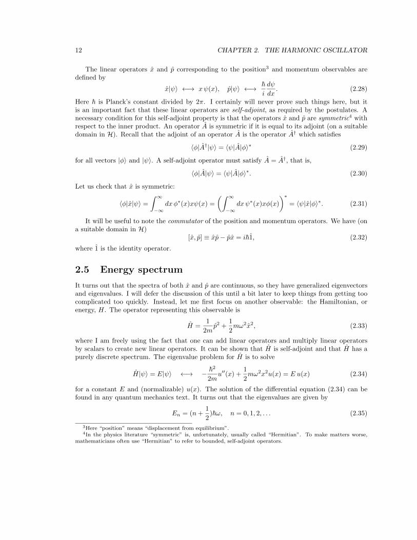
The linear operators x and p corresponding to the position3 and momentum observables aredefined by
x|ψ〉 ←→ xψ(x), p|ψ〉 ←→ ~i
dψ
dx. (2.28)
Here ~ is Planck’s constant divided by 2π. I certainly will never prove such things here, but itis an important fact that these linear operators are self-adjoint, as required by the postulates. Anecessary condition for this self-adjoint property is that the operators x and p are symmetric4 withrespect to the inner product. An operator A is symmetric if it is equal to its adjoint (on a suitabledomain in H). Recall that the adjoint of an operator A is the operator A† which satisfies
〈φ|A†|ψ〉 = 〈ψ|A|φ〉∗ (2.29)
for all vectors |φ〉 and |ψ〉. A self-adjoint operator must satisfy A = A†, that is,
〈φ|A|ψ〉 = 〈ψ|A|φ〉∗. (2.30)
Let us check that x is symmetric:
〈φ|x|ψ〉 =
∫ ∞−∞
dxφ∗(x)xψ(x) =
(∫ ∞−∞
dxψ∗(x)xφ(x)
)∗= 〈ψ|x|φ〉∗. (2.31)
It will be useful to note the commutator of the position and momentum operators. We have (ona suitable domain in H)
[x, p] ≡ xp− px = i~1, (2.32)
where 1 is the identity operator.
2.5 Energy spectrum
It turns out that the spectra of both x and p are continuous, so they have generalized eigenvectorsand eigenvalues. I will defer the discussion of this until a bit later to keep things from getting toocomplicated too quickly. Instead, let me first focus on another observable: the Hamiltonian, orenergy, H. The operator representing this observable is
H =1
2mp2 +
1
2mω2x2, (2.33)
where I am freely using the fact that one can add linear operators and multiply linear operatorsby scalars to create new linear operators. It can be shown that H is self-adjoint and that H has apurely discrete spectrum. The eigenvalue problem for H is to solve
H|ψ〉 = E|ψ〉 ←→ − ~2
2mu′′(x) +
1
2mω2x2u(x) = E u(x) (2.34)
for a constant E and (normalizable) u(x). The solution of the differential equation (2.34) can befound in any quantum mechanics text. It turns out that the eigenvalues are given by
En = (n+1
2)~ω, n = 0, 1, 2, . . . (2.35)
3Here “position” means “displacement from equilibrium”.4In the physics literature “symmetric” is, unfortunately, usually called “Hermitian”. To make matters worse,
mathematicians often use “Hermitian” to refer to bounded, self-adjoint operators.

2.5. ENERGY SPECTRUM 13
The “quantum number” n is the number of “quanta” of energy ~ω the oscillator has relative to itslowest energy state – or “ground state”. The corresponding eigenvectors correspond to functionswhich are polynomials in x times a Gaussian in x. Explicitly:
|En〉 ←→ un(x) =1√
2nn!
(mωπ~
) 14
e−mω2~ x
2
Hn(
√mω
~x), (2.36)
where Hn(ξ) is the Hermite polynomial in ξ,
Hn(ξ) = (−1)neξ2 dn
dξne−ξ
2
, n = 0, 1, 2, . . . (2.37)
Examples of Hermite polynomials are
H0(ξ) = 1, H1(ξ) = 2ξ, H2(ξ) = 4ξ2 − 2. (2.38)
The energy eigenvectors are orthonormal:
〈En|Em〉 = δnm. (2.39)
Because H is self-adjoint its eigenvectors form an orthonormal basis for the Hilbert space H.This means that any element of the Hilbert space can be written as a superposition of energyeigenvectors, that is, there exist complex constants cn such that5
|ψ〉 =
∞∑n=0
cn|En〉. (2.40)
Here cn = 〈En|ψ〉 are the components of |ψ〉 in the basis of energy eigenvectors. Alternatively, wehave the operator identity ∑
k
|Ek〉〈Ek| = 1, (2.41)
so that
|ψ〉 =
(∑k
|Ek〉〈Ek|
)|ψ〉 =
∑k
|Ek〉〈Ek|ψ〉 =∑k
ck|Ek〉. (2.42)
The normalization of |ψ〉, coupled with the orthonormality of the basis |En〉, means
〈ψ|ψ〉 =
∞∑n=0
|cn|2 = 1. (2.43)
In light of (2.40), knowing the sequence of complex numbers c0, c1, c2, . . . is the same as knowingthe state vector |ψ〉. Using the energy eigenvectors the Hilbert space of square integrable functioncan be identified with the set of square-summable sequences of complex numbers.
According to the rules of quantum mechanics, we can interpret |cn|2 as the probability that theenergy En is measured when the oscillator is in the state given by |ψ〉. The normalization condition
5The infinite series converges to |ψ〉 in the sense that the difference of |ψ〉 and the sequence of partial sums fromthe right hand side define a vector with zero norm.

14 CHAPTER 2. THE HARMONIC OSCILLATOR
(2.43) then guarantees that the probabilities for all possible outcomes of an energy measurementadd up to one.
The complex amplitudes for the oscillator can be viewed as a “classical limit” of operators whichhave an important meaning relative to the energy spectrum. These operators are a and a†, definedby
a =
√mω
2~(x+
i
mωp), a† =
√mω
2~(x− i
mωp). (2.44)
Note that I have inserted a convenient factor of 1√~ into the definition of each operator relative to
its classical counterpart. This redefinition makes the amplitudes dimensionless. Because x and pare self-adjoint, you can see from inspection that a and a† are adjoints of each other. Using thecommutation relations between position and momentum it is easy to see that
[a, a†] = 1 (2.45)
and
H = ~ω(a†a+1
21). (2.46)
The operator 12~ω1 represents a simple shift of the zero point of energy from zero. One can drop
this term if so desired; this amounts to measuring the energy of the oscillator relative to its groundstate energy. The operator N ≡ a†a represents the energy quanta observable; it is also called thenumber operator. I say this since
N |En〉 = n|En〉. (2.47)
Notice in particular that the ground state satisfies
N |E0〉 = 0, =⇒ 〈E0|a†a|E0〉 = 0. (2.48)
The second equation says that the norm of the vector a|E0〉 vanishes, which also implies the firstequation. Therefore the ground state is characterized by the condition
a|E0〉 = 0. (2.49)
More generally, it is easy to compute:
[N , a] = −a, [N , a†] = a†. (2.50)
This implies that a|En〉 ∝ |En−1〉 and a†|En〉 ∝ |En+1〉. Explicit computation reveals
a|En〉 =√n|En−1〉, a†|En〉 =
√n+ 1|En+1〉, n = 1, 2, . . . (2.51)
For this reason the operators a, a† are sometimes called “ladder operators”, or “annihilation andcreation operators” of energy quanta. These operators, mathematically speaking, add and subtractenergy quanta from energy eigenstates. It is possible to derive the energy spectrum – including theenergy eigenfunctions – just using the commutation relation of N , a, and a†. The algebra of theladder operators more or less defines the quantum oscillator.

2.6. POSITION, MOMENTUM, AND THEIR CONTINUOUS SPECTRA 15
2.6 Position, momentum, and their continuous spectra
The mathematical model of operators representing observables with continuous spectra, e.g., theposition and momentum operators, is a little more complicated than that for operators representingobservables with discrete spectrum such as the oscillator energy. Operators with discrete spectrumare in many ways like ordinary matrices, albeit with an infinity of matrix elements. Operators withcontinuous spectrum require some new technology. Let us begin by seeing the difficulties whicharise when trying to solve the eigenvalue problem for operators such as position and momentum.
2.6.1 Position
The eigenvalue problem for the operator representing position should be
x|y〉 = y|y〉 ←→ xψy(x) = yψy(x), (2.52)
where y is some (hopefully real) number. No non-trivial function can satisfy this condition. Indeed,if the function is non-zero for at least two values of x there can be no solution. But if the function isnon-zero for only one value of x then it is (equivalent to) the zero vector in the Hilbert space. It ispossible to solve this position eigenvalue equation if one allows a more general type of eigenfunction,a “generalized function”, the Dirac delta function δ(x, y). The solution of the eigenvalue equationis then written
ψy(x) = δ(x, y). (2.53)
We shall need some of this technology, so let us digress briefly to review it.Strictly speaking, the Dirac delta function is not a function, but rather a distribution.6 It is
possible to treat the Dirac delta as a limit of suitable elements of the Hilbert space. The limit willnot exist in the Hilbert space, but the limit of suitable scalar products will exist, and that is all weshall need since the probability interpretation only needs a way to define the scalar products 〈y|ψ〉for all possible values of y. A standard example of this limiting process is as follows. Let y be somegiven real number and consider the following 1-parameter family of elements of H:
|φε,y〉 ←→ φε,y(x) =1
2π
∫ 1ε
− 1ε
dk eik(x−y), ε > 0. (2.54)
It is straightforward to compute the integral and find
|φε,y(x)|2 =sin2
(πε (x− y)
)π2(x− y)2
, (2.55)
from which you can see that the function φε,y(x) is square integrable; indeed for any ε > 0:
〈φε,y|φε,y〉 =
∫ ∞−∞|φε,y(x)|2 =
1
ε. (2.56)
The eigenfunction of position – the delta function – arises in the limit as ε→ 0. Although we oftenstate this result by writing
δ(x, y) =1
2π
∫ ∞−∞
dk eik(x−y), (2.57)
6Here, a distribution is a continuous linear function on a dense subspace S ⊂ H of the Hilbert space, where“continuous” implies a choice of appropriate appropriate topology on S. I shall generally avoid this more rigorousway of doing things.

16 CHAPTER 2. THE HARMONIC OSCILLATOR
this equation has to be treated carefully. What it means is that for vectors |χ〉 in a suitable subspaceS ⊂ H the limit of 〈φε,y|χ〉 as ε→ 0 is defined. We have
〈φε,y|χ〉 =1
2π
∫ ∞−∞
dx
∫ 1ε
− 1ε
dk e−ik(x−y)χ(x). (2.58)
For suitably nice functions7 one can interchange the orders of integration and then take the limitas ε→ 0. After interchanging the order of integration we get
〈φε,y|χ〉 =1
2π
∫ 1ε
− 1ε
dk
∫ ∞−∞
dx e−ik(x−y)χ(x) =1
2π
∫ 1ε
− 1ε
dk χ(k)eiky, (2.59)
where χ(k) is the Fourier transform of χ(x). As ε → 0 we get the Fourier representation of thefunction χ(y):
limε→0〈φε,y|χ〉 =
1
2π
∫ ∞−∞
dk χ(k)eiky = χ(y). (2.60)
So, we have
limε→0
∫ ∞−∞
dxφ∗ε,y(x)χ(x) = χ(y), (2.61)
which is the defining relation for the delta function.If desired, one can opt to avoid all this delta function stuff and always work with a small but
non-vanishing ε. Then the position will not be defined as a mathematical point, but only in termsof a region of size determined by ε, but if ε is small enough it will not matter physically. Whilethis is satisfying in that one does not need to introduce distributions, this framework is somewhatcumbersome, of course, and that is why one likes to set ε = 0 and use the delta function.
The preceding results are usually packaged in various simple notations. If you know what youare doing, these notations are very helpful. If you let the notation substitute for understanding,then eventually there will be trouble. The most common notational slogans are:
1
2π
∫ ∞−∞
dk eik(x−y) = δ(x, y) = δ(y, x) ≡ δ(x− y), (2.62)
∫ ∞−∞
dx δ(x, y)f(x) = f(y), (2.63)
f(x)δ(x, y) = f(y)δ(x, y), (2.64)
limε→0|φε,y〉 = |y〉, (2.65)
|y〉 ←→ δ(x, y), (2.66)
x|y〉 = y|y〉, (2.67)
7For our purposes, a class of “nice” functions would be smooth functions whose absolute value decreases fasterthan the reciprocal of any polynomial in x as |x| → ∞.

2.6. POSITION, MOMENTUM, AND THEIR CONTINUOUS SPECTRA 17
〈y|χ〉 = χ(y), (2.68)
∫ ∞−∞
dy χ(y)|y〉 = |χ〉, (2.69)
〈y|z〉 = δ(y, z), (2.70)
∫ ∞−∞
dx |x〉〈x| = 1. (2.71)
These last five formal relations are the most important for us. If we augment our Hilbert spaceby including generalized functions like the delta function then the eigenvectors of position canbe accommodated and they constitute a generalization of an orthonormal basis, now labeled bya continuous variable instead of a discrete variable, with summations over eigenvectors becomingintegrals, and with the Dirac delta function replacing the Kronecker delta in the orthonormalityrelation.
It will be useful later to have available the following identities which are satisfied by the energyeigenvectors and position eigenvectors:∫ ∞
−∞dxu∗k(x)ul(x) =
∫ ∞−∞
dx 〈Ek|x〉〈x|El〉 = 〈Ek|El〉 = δkl, (2.72)
∑k
u∗k(x)uk(y) =∑k
〈y|Ek〉〈Ek|x〉 = 〈y|x〉 = δ(x, y). (2.73)
Finally, I remind you the physical interpretation of the (position) wave function,
|ψ〉 ←→ ψ(x) = 〈x|ψ〉. (2.74)
The probability Px(a, b) for finding the position x ∈ (a, b) is given by
Px(a, b) =
∫ b
a
dx |ψ(x)|2. (2.75)
We say that |ψ(x)|2 is the probability density for position, and that |ψ(x)|2dx is the probability forfinding the particle in the infinitesimal interval (x, x+ dx) .
2.6.2 Momentum
For the momentum operator we want to solve an eigenvalue problem of the form
p|p〉 = p|p〉 ←→ ~i
d
dxup(x) = pup(x), (2.76)
where p is (hopefully) a real constant. It is not too hard to solve this differential equation; we have
up(x) = Aei~px, (2.77)

18 CHAPTER 2. THE HARMONIC OSCILLATOR
where A is a constant. There are two difficulties here. First of all, the spectrum of the momentumoperator should consist of real numbers, but the eigenvalue equation allows p to be complex. Sec-ondly, and perhaps more drastically, whether p is real or complex (assuming A 6= 0) the functionup(x) is not square-integrable – it is not an element of the Hilbert space. We are in a similar placeas we were with the position operator, and we can proceed in a similar way. Once again we candefine the eigenfunction as a generalized function (or “distribution) via a limit of elements of H.
Fix a real number p and consider a 1-parameter family of vectors in H:
|µp,ε〉 ←→ up,ε(x) =1√2π~
ei~pxe−ε
2x2
, ε > 0. (2.78)
It is easy to see that these functions are square-integrable for any ε > 0:
〈µp,ε|µp,ε〉 =1
4~
√2
π
1
ε. (2.79)
Of course, up,ε(x) is not a momentum eigenfunction, but it does approach the “generalized” eigen-function (2.77) as ε → 0. While the limit does not lead to an element of H, scalar products withelements of H do admit a limit. We have
〈µp,ε|ψ〉 =1√2π~
∫ ∞−∞
dx e−i~pxe−ε
2x2
ψ(x). (2.80)
Evidently, as ε→ 0 the limit of the scalar product is proportional to the Fourier transform ψ of ψ:
limε→0〈µp,ε|ψ〉 =
1√2π~
∫ ∞−∞
dx e−i~pxψ(x) =
1√~ψ(k), k = p/~. (2.81)
One usually uses a notation such as φ(p) = 1√~ ψ(k) and calls φ(p) the momentum wave function.
Since knowing the Fourier transform of a function is as good as knowing the function, and sincethe Fourier transform ψ is square-integrable if and only if ψ is, we could define H as the set ofsquare-integrable momentum wave functions. This is the basis for using momentum space wavefunctions to “do” quantum mechanics.
As with the technology surrounding generalized position eigenvectors, the preceding results arepackaged in various simple notations. The most common are:
limε→0|µp,ε〉 = |p〉 ←→ lim
ε→0up,ε(x) ≡ up(x) =
1√2π~
ei~px, (2.82)
p|p〉 = p|p〉 (2.83)
〈p|ψ〉 =1√~ψ(p/~) = φ(p), (2.84)
〈x|p〉 =1√2π~
ei~px, 〈p|x〉 =
1√2π~
e−i~px, (2.85)
∫ ∞−∞
dp φ(p)|p〉 = |ψ〉. (2.86)

2.6. POSITION, MOMENTUM, AND THEIR CONTINUOUS SPECTRA 19
〈p′|p〉 = δ(p′, p), (2.87)
∫ ∞−∞
dp |p〉〈p| = 1. (2.88)
There are relations involving the energy eigenvectors analogous to what we had when discussingthe position eigenvectors:∫ ∞
−∞dp u∗k(p)ul(p) =
∫ ∞−∞
dp 〈Ek|p〉〈p|El〉 = 〈Ek|El〉 = δkl, (2.89)
∑k
u∗k(p)uk(p′) =∑k
〈p′|Ek〉〈Ek|p〉 = 〈p′|p〉 = δ(p, p′). (2.90)
Finally, I remind you the physical interpretation of the momentum wave function,
|ψ〉 ←→ φ(p) = 〈p|ψ〉 =1√~ψ(p/~). (2.91)
The probability Pp(a, b) for finding the momentum in the range (a, b) is given by
Pp(a, b) =
∫ b
a
dp |φ(p)|2. (2.92)
2.6.3 General formalism
Let us now create a little formalism to summarize these results and to generalize them to otherobservables which may have a continuous part to their spectrum. All this formalism can be justifiedusing the spectral theory of self-adjoint operators on Hilbert space.
Let A be a self-adjoint operator on a Hilbert space H. Its spectrum can consist of a discretepart,
A|an〉 = an|an〉, n = 1, 2, . . . , an ∈ R (2.93)
and a continuous part,A|λ〉 = λ|λ〉, λ ∈ U ⊂ R. (2.94)
The eigenvectors |an〉 are elements of H and can be chosen to be orthonormal
〈am|an〉 = δmn. (2.95)
The |λ〉 are limits of elements of H but are not themselves elements of H. The limits of the scalarproducts of |λ〉 with a (dense) subspace of H will exist. These “generalized eigenvectors” will beorthonormal “in the delta function sense”:
〈λ′|λ〉 = δ(λ′, λ). (2.96)
The eigenvectors and generalized eigenvectors together form a basis for the Hilbert space in thesense that for any |ψ〉 ∈ H
|ψ〉 =∑n
ψn|an〉+
∫U
dλψ(λ)|λ〉. (2.97)

20 CHAPTER 2. THE HARMONIC OSCILLATOR
Equivalently,
1 =∑n
|an〉〈an|+∫U
dλ |λ〉〈λ|. (2.98)
Given the “spectral decomposition” (2.97), if the state vector of the system is |ψ〉, the interpretationof ψn is that |ψn|2 is the probability the system will be found to have the value an (in the state |an〉)for the observable represented by A. If the eigenvalue an is degenerate – there is more than onelinearly independent eigenvector with eigenvalue an for A – then the total probability for gettingan upon a measurement of A is obtained by summing |ψn|2 over the degenerate subspace. The
interpretation of ψ(λ) is that∫ badλ |ψ(λ)|2 is the probability for measuring A and getting the value
λ ∈ (a, b). If the generalized eigenvalues are degenerate one must sum/integrate this quantity overthe (generalized) eigenspace to get the total probability.
Some self-adjoint operators have purely discrete spectrum; the Hamiltonian for the harmonicoscillator is an example. Other operators, like the position and momentum have purely continuousspectrum. Operators also may have both continuous and discrete parts to their spectrum. Anexample of this would be the Hamiltonian for a hydrogen atom, where the bound states – the usualatomic energy levels – correspond to the discrete spectrum and the scattering (or ionized) statescorrespond to the continuous spectrum.
2.7 Time evolution
Next we will briefly review the dynamics of a quantum oscillator in each of the Schrodinger andHeisenberg pictures. I will need the Heisenberg picture later since this picture of dynamics is themost immediately accessible in quantum field theory. You should be familiar with the equivalentSchrodinger picture of dynamics, so we can start there.
The time evolution of a state vector in the Schrodinger picture is, of course, defined by theSchrodinger equation:
H|ψ(t)〉 = i~d
dt|ψ(t)〉. (2.99)
Assuming that the Hamiltonian has no explicit time dependence, as is the the case for the harmonicoscillator, the solution to this equation for a given initial state |ψ(0)〉 can be expressed as
|ψ(t)〉 = e−i~ tH |ψ(0)〉. (2.100)
You may be more familiar with an alternative – but equivalent – form of this solution. If the initialvector is expanded in a basis of energy eigenvectors:
|ψ(0)〉 =∑n
cn|En〉, (2.101)
then (2.100) takes the form
|ψ(t)〉 =∑n
cne− i
~Ent|En〉. (2.102)
In the Schrodinger picture, observables A are constructed as operators built from x and p. Wewrite A = A(x, p), and the expectation value of A at time t, denoted by 〈A〉(t) is calculated by
〈A〉(t) = 〈ψ(t)|A|ψ(t)〉. (2.103)

2.7. TIME EVOLUTION 21
As you may know, all physical predictions of quantum mechanics can be expressed in terms ofexpectation values of suitable observables, so (2.103) suffices to provide all dynamical information.
The Heisenberg picture of dynamics can be understood as arising from a different organizationof terms in the fundamental formula (2.103). We write
〈A〉(t) = 〈ψ(t)|A|ψ(t)〉 = 〈ψ(0)|e i~ tHAe− i~ tH |ψ(0)〉 ≡ 〈ψ(0)|A(t)|ψ(0)〉, (2.104)
where I’ve definedA(t) = e
i~ tHAe−
i~ tH . (2.105)
You can see that using the last equality in (2.104) along with (2.105) amounts to assigning thetime dependence to the operator rather than to the state vector. The only thing that matters,physically speaking, is the combination of factors which appears in (2.104), so the organization ofthe time dependence within this expression is a matter of convenience only. Evidently, we can viewthe mathematical representation of the time evolution of any observable either as a one parameterfamily of state vectors with a fixed operator representing the observable, or as a one parameter familyof operator representatives of the observable and a fixed state vector. The former organization ofthe mathematics is the Schrodinger picture and the latter organization is the Heisenberg picture.In the Heisenberg picture the operator A(t) represents the observable A at time t. From (2.105)you can see that in general the Heisenberg picture operator(s) for the observable A will be the sameas the Schrodinger picture operator for A at a single time, which has been chosen to be t = 0.
You might find the Heisenberg picture is more closely aligned with how you learned to thinkabout dynamics in Newtonian mechanics. There we always speak of the time evolution of observ-ables like position and momentum. In the Heisenberg picture of quantum mechanics we do thesame thing with the operators representing the observables. In the Heisenberg picture there is noSchrodinger equation – the state vector is the same for all time, and it is determined once and for allby initial conditions. The equations governing time evolution are of the form (2.105). For a systemlike the harmonic oscillator, all observables are built from x and p, so it suffices to understand
x(t) = ei~ tH xe−
i~ tH , p(t) = e
i~ tH pe−
i~ tH , (2.106)
in order to understand the time evolution of the oscillator in the Heisenberg picture. These relationscan be expressed as differential equations, just as (2.100) can be expressed as (2.99). You can checkthat if the definitions of x(t) and p(t) are differentiated with respect to time then the result is
d
dtx(t) =
1
i~[x(t), H],
d
dtp(t) =
1
i~[p(t), H]. (2.107)
These are the Heisenberg equations of motion. They can be considered the quantum versions ofHamilton’s equations. In this analogy, the operators represent the classical position and momentumvariables, and the commutator represents the Poisson bracket. To see this a little more clearly, weneed to compute the commutators appearing in (2.107). This can be done by noting that for anyoperator A(t) we have
[A(t), H] = [ei~ tHA(0)e−
i~ tH , H] = e
i~ tH [A(0), H]e−
i~ tH = [A(0), H](t). (2.108)
Applying this to the displacement and momentum for a harmonic oscillator gives
[x(t), H] =i~mp(t), [p(t), H] = −i~mω2x(t), (2.109)

22 CHAPTER 2. THE HARMONIC OSCILLATOR
so thatd
dtx(t) =
1
mp(t),
d
dtp(t) = −mω2x(t), (2.110)
which have the same form as Hamilton’s equations for a harmonic oscillator. Consequently, theseequations are straightforward to solve:
x(t) = cos(ωt) x+1
mωsin(ωt) p, p(t) = cos(ωt) p−mω sin(ωt) x. (2.111)
Here I have used the identification
x(0) = x, p(0) = p. (2.112)
As you can see, the Heisenberg operators evolve in time in the same way as their classical counter-parts. You can also see how the Heisenberg operators are the same as the Schrodinger operator atthe time t = 0.
From the forms of x(t) and p(t) we easily compute the Heisenberg form of the creation andannihilation operators a = a(0), a† = a†(0). We have
a(t) =
√mω
2~(x(t) +
i
mωp(t)) = e−iωta (2.113)
and
a†(t) =
√mω
2~(x(t)− i
mωp(t)) = eiωta†, (2.114)
as you might have anticipated based upon the classical analogs of these formulas.Finally, it is straightforward to calculate the Heisenberg form of the Hamiltonian:
H(t) =1
2mp2(t) +
1
2mω2x2(t) =
1
2mp2(0) +
1
2mω2x2(0) =
1
2mp2 +
1
2mω2x2, (2.115)
or
H(t) = ~ω(a†(t)a(t) +1
21) = ~ω(a†(t)a(t) +
1
21) = ~ω(a†a+
1
21). (2.116)
Evidently, the Heisenberg form of the Hamiltonian operator is the same as its Schrodinger form.This is because
H(t) = ei~ HtHe−
i~ Ht = H (2.117)
owing to the fact that[H, f(H)] = 0 (2.118)
for any function f of H. This result, H(t) = H(0), is equivalent to conservation of energy for thequantum oscillator.
2.8 Coherent States
It will be worth mentioning a family of states that is useful for making the connection betweenthe classical and quantum oscillator. These are the coherent states, mathematically defined aseigenvectors of the lowering operator a:
a|z〉 = z|z〉. (2.119)

2.9. PROBLEMS 23
Note that a is not symmetric and its eigenvalues are in general complex. Indeed, it can be shownthat there is a coherent state associated to any complex number z. Since a is not self-adjoint, theusual issues with generalized eigenvectors and continuous spectrum do not occur; these vectors arein the Hilbert space and can be normalized in the usual way. However, they are not orthogonalfor different eigenvalues. The coherent states are over-complete, which means that they span theHilbert space but they are not all linearly independent. It can be shown that the coherent stateshave non-zero probabilities for all energies to occur.
The coherent states enjoy a number of important properties. The real and imaginary parts ofthe eigenvalues yield the expectation values of position and momentum:
〈z|x|z〉 =
√2~mω<(z), 〈z|p|z〉 =
√2~mω=(z). (2.120)
All of these states are minimum uncertainty states:
(∆x)2 = 〈z|x2|z〉 − 〈z|x|z〉2 =~
2mω, (2.121)
(∆p)2 = 〈z|p2|z〉 − 〈z|p|z〉2 =~mω
2, (2.122)
∆x∆p =~2. (2.123)
Finally, if the oscillator is in a coherent state defined by z at time t = 0, then at time t it is inthe coherent state defined by ze−iωt. This last fact is very easy to see in the Heisenberg picture.This means that the complex eigenvalue z evolves in time in the same way as the classical complexamplitude a, defined in (5.98).
The coherent states can be viewed as states which are “closest to classical” in that the positionand momentum have the minimum possible uncertainty and their expectation values evolve accord-ing to the classical equations of motion (as they must by Ehrenfest’s theorem). For macroscopicvalues of mass and frequency, these states represent classical Newtonian behavior to good accuracy.
2.9 Problems
1. A system with 2 degrees of freedom, labeled x and y, has the following Lagrangian:
L =1
2m(x2 + y2)− α(x2 + y2)− β(x− y)2.
Find the point or points of stable equilibrium. Find the normal modes and characteristicfrequencies of oscillation about the equilibria.
2. Prove the result quoted in the text concerning simultaneous diagonalization of quadratic forms.
Hints: (1) The quadratic form M defining the approximate kinetic energy can be used to definea scalar product (~v, ~w) ≡ M(~v, ~w) = viwjMij = vTMw. (2) Every scalar product allows alinear change of basis to an orthonormal basis ~ei in which (~ei, ~ej) = δij . (3) The orthonormal
basis is unique up to any change of basis ~ei → Oji~ej where O is an orthogonal matrix,OT = O−1. The potential energy quadratic form is defined by a symmetric array K. Under a

24 CHAPTER 2. THE HARMONIC OSCILLATOR
change of orthonormal basis defined by O the array changes by K → OTKO = O−1KO. (4)Use the linear algebra result that any symmetric array, such as K, can be diagonalized via asimilarity transformation by an orthogonal matrix.
3. Show that the momentum (2.28) and Hamiltonian (2.33) are symmetric operators.
4. Show that the time evolution defined by the Schrodinger equation (2.99) preserves the nor-malization of the state vector:
d
dt〈ψ(t)|ψ(t)〉 = 0.
5. Show that the linear operations defined in (2.51) satisfy the adjoint relation (2.29). (Hint: Itis sufficient to check the relation on a basis.)
6. Using the probability interpretation of the state vector, show that the expectation value – thestatistical mean – of an observable A in a state represented by |ψ〉 can be calculated by
〈A〉 = 〈ψ|A|ψ〉.
7. Define the projection operator into the ground state for the harmonic oscillator by
P0|ψ〉 = 〈E0|ψ〉|E0〉.
Show that this is a linear operator. Show that this operator is symmetric. Find the eigenvaluesand eigenvectors of this operator. Show that the expectation value in the state |ψ〉 of P0 isthe probability that an energy measurement in the state represented by |ψ〉 results in theground state energy. (In this fashion all probabilities in quantum mechanics can be reducedto computations of expectation values of suitable observables. )
8. The momentum representation for quantum mechanics uses the Fourier transform to iden-tify the Hilbert space H with square integrable functions of momentum. In the momentumrepresentation the position and momentum operators are given by
pφ(p) = pφ(p), xφ(p) = i~d
dpφ(p).
Show that these operators satisfy the commutation relations (2.32). Express the harmonic os-cillator Hamiltonian as an operator on momentum wave functions. Using the known spectrumof this Hamiltonian in the position representation, (2.35) and (2.36), deduce the spectrum ofthe Hamiltonian in the momentum representation. (Hint: You do not have to take any Fouriertransforms.)
9. Find the ground and first excited states of the oscillator in the momentum representation bytaking the Fourier transform of the position representation wave functions.

2.9. PROBLEMS 25
10. The uncertainty in an observable A in a given state is defined to be the standard deviation∆A of (an arbitrarily large number of) measurements of that observable in an ensemble ofsystems in the same state. Given a state vector |ψ〉 the uncertainty can be computed via
(∆A)2 = 〈A2〉 − 〈A〉2 = 〈ψ|A2|ψ〉 − 〈ψ|A|ψ〉2.
For the ground state of the harmonic oscillator calculate ∆H, ∆x and ∆p.
11. At t = 0 a harmonic oscillator is in the state
|ψ(0)〉 = cos a|E0〉+ sin a|E1〉,
where a is some real number. Calculate 〈x〉(t), the expectation value of displacement as afunction of time.
12. What are the eigenvalues of the kinetic and potential energies for a harmonic oscillator? Whydon’t they add up to give the discrete spectrum of energies?
13. For a quantum oscillator, consider eigenvectors of the annihilation operator:
a|z〉 = z|z〉.
Show that for any z ∈ C there is a normalized eigenvector
|z〉 = e−|z|2/2eza
†|E0〉. (2.124)
Prove that there are no eigenvectors of a†. Verify the uncertainties (2.121) and (2.122).Show that the probability Pn(z) for getting n energy quanta in the state |z〉 is the Poissondistribution
Pz(n) = e−|z|2 |z|2n
n!. (2.125)
Finally, show from the Poisson distribution that in a coherent state defined by z the meannumber of energy quanta is
〈n〉 =
∞∑n=0
nPz(n) = |z|2.
14. For a quantum oscillator, define new creation and annihilation operators via
b = λa+ νa†, b† = λa† + νa,
where λ and ν are any two real numbers satisfying
λ2 − ν2 = 1.
Show that [b, b†] = 1. Show that in the state |0〉 of vanishing quanta according to b,
b|0〉 = 0,

26 CHAPTER 2. THE HARMONIC OSCILLATOR
the variances in the displacement and momenta satisfy
(∆x)2 =~
2mω(λ− ν)2, (∆p)2 =
~mω2
(λ+ ν)2
so that
(∆x)2(∆p)2 =~2
4.
This property extends to all the coherent states defined by b; such states are called squeezedstates.

Chapter 3
Tensor Products and IdenticalParticles
As we shall see, in a certain sense the simplest incarnation of a quantum field is just an infinitecollection of harmonic oscillators. We certainly understand the quantum mechanics of a singleoscillator. How do we use this information to understand a system consisting of two or morequantum oscillators? The tensor product is the construction we need. In quantum mechanics wealways use the tensor product construction to build a composite system (e.g., many oscillators)from a combination of subsystems (e.g., a single oscillator). This chapter will explain all this.
3.1 Definition of the tensor product
Let us consider the quantum theory of a system consisting of 2 independent oscillators characterizedby masses m1 and m2 and frequencies ω1 and ω2. (I remind you that the motion of any dynamicalsystem with 2 degrees of freedom near stable equilibrium can be described by two such oscillators.)Conceptually at least, it is not hard to describe the quantum structure of the system. For themost part one just considers two copies of the quantum oscillator described in the last chapter. Forexample, the states of the composite system are obtained by (superpositions of) pairs of vectors,|ψ1〉, |ψ2〉, coming from two Hilbert spaces, H1, H2 of square-integrable functions, ψ1(x1), ψ2(x2).But how does this exactly fit into the quantum postulates involving a Hilbert space, self-adjointoperators, and all that? This question is answered via the tensor product construction.1
Consider any two Hilbert spaces H1 and H2, with elements denoted by |ψ〉1 and |φ〉2, respec-tively. I will give you two equivalent ways of defining the tensor product. One is simpler than theother, but they both have their advantages and we will definitely want to have both points of view.
First definitionLet |ei〉, i = 1, 2, . . . , n1, and |fa〉, a = 1, 2, . . . , n2, be bases for each of the Hilbert spaces.2
1The tensor product is also known as the “direct product”. It is related to – but is different from – the “Cartesianproduct”.
2The ability to find a basis which is in 1-1 correspondence with the set of integers is a slight restriction on theallowed Hilbert spaces to the class of separable Hilbert spaces. It is not necessary that the Hilbert spaces are separablefor what will follow, but for convenience I will suppose that they are separable.
27
28 CHAPTER 3. TENSOR PRODUCTS AND IDENTICAL PARTICLES
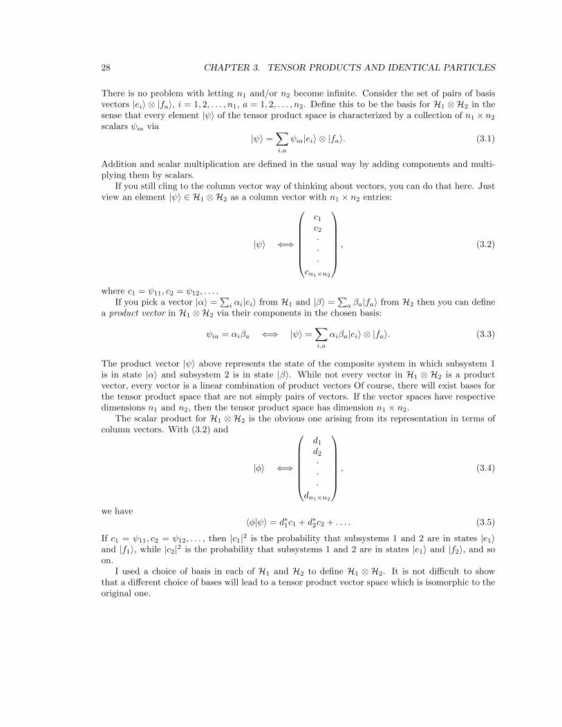
There is no problem with letting n1 and/or n2 become infinite. Consider the set of pairs of basisvectors |ei〉 ⊗ |fa〉, i = 1, 2, . . . , n1, a = 1, 2, . . . , n2. Define this to be the basis for H1 ⊗H2 in thesense that every element |ψ〉 of the tensor product space is characterized by a collection of n1 × n2scalars ψia via
|ψ〉 =∑i,a
ψia|ei〉 ⊗ |fa〉. (3.1)
Addition and scalar multiplication are defined in the usual way by adding components and multi-plying them by scalars.
If you still cling to the column vector way of thinking about vectors, you can do that here. Justview an element |ψ〉 ∈ H1 ⊗H2 as a column vector with n1 × n2 entries:
|ψ〉 ⇐⇒
c1c2···
cn1×n2
, (3.2)
where c1 = ψ11, c2 = ψ12, . . . .If you pick a vector |α〉 =
∑i αi|ei〉 from H1 and |β〉 =
∑a βa|fa〉 from H2 then you can define
a product vector in H1 ⊗H2 via their components in the chosen basis:
ψia = αiβa ⇐⇒ |ψ〉 =∑i,a
αiβa|ei〉 ⊗ |fa〉. (3.3)
The product vector |ψ〉 above represents the state of the composite system in which subsystem 1is in state |α〉 and subsystem 2 is in state |β〉. While not every vector in H1 ⊗ H2 is a productvector, every vector is a linear combination of product vectors Of course, there will exist bases forthe tensor product space that are not simply pairs of vectors. If the vector spaces have respectivedimensions n1 and n2, then the tensor product space has dimension n1 × n2.
The scalar product for H1 ⊗ H2 is the obvious one arising from its representation in terms ofcolumn vectors. With (3.2) and
|φ〉 ⇐⇒
d1d2···
dn1×n2
, (3.4)
we have〈φ|ψ〉 = d∗1c1 + d∗2c2 + . . . . (3.5)
If c1 = ψ11, c2 = ψ12, . . . , then |c1|2 is the probability that subsystems 1 and 2 are in states |e1〉and |f1〉, while |c2|2 is the probability that subsystems 1 and 2 are in states |e1〉 and |f2〉, and soon.
I used a choice of basis in each of H1 and H2 to define H1 ⊗ H2. It is not difficult to showthat a different choice of bases will lead to a tensor product vector space which is isomorphic to theoriginal one.
3.1. DEFINITION OF THE TENSOR PRODUCT 29
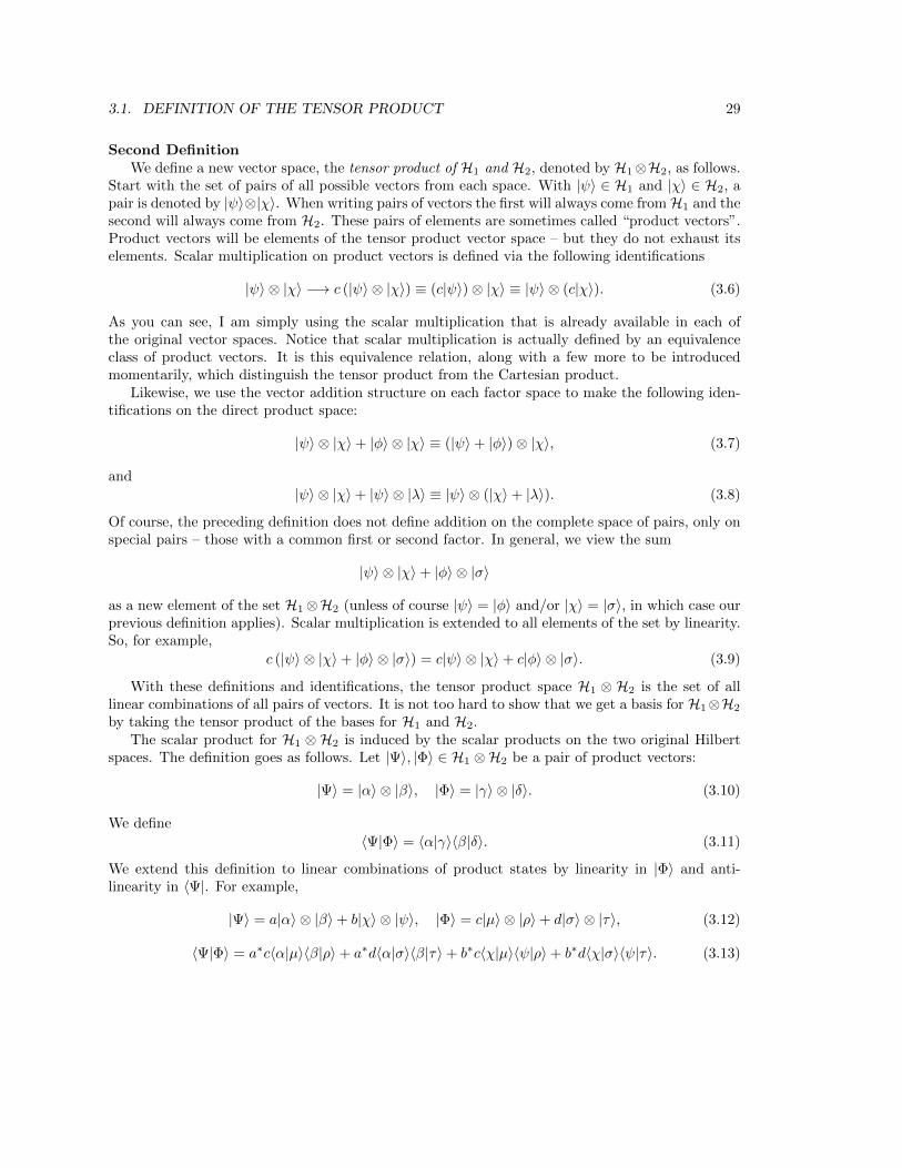
Second DefinitionWe define a new vector space, the tensor product of H1 and H2, denoted by H1⊗H2, as follows.
Start with the set of pairs of all possible vectors from each space. With |ψ〉 ∈ H1 and |χ〉 ∈ H2, apair is denoted by |ψ〉⊗|χ〉. When writing pairs of vectors the first will always come fromH1 and thesecond will always come from H2. These pairs of elements are sometimes called “product vectors”.Product vectors will be elements of the tensor product vector space – but they do not exhaust itselements. Scalar multiplication on product vectors is defined via the following identifications
|ψ〉 ⊗ |χ〉 −→ c (|ψ〉 ⊗ |χ〉) ≡ (c|ψ〉)⊗ |χ〉 ≡ |ψ〉 ⊗ (c|χ〉). (3.6)
As you can see, I am simply using the scalar multiplication that is already available in each ofthe original vector spaces. Notice that scalar multiplication is actually defined by an equivalenceclass of product vectors. It is this equivalence relation, along with a few more to be introducedmomentarily, which distinguish the tensor product from the Cartesian product.
Likewise, we use the vector addition structure on each factor space to make the following iden-tifications on the direct product space:
|ψ〉 ⊗ |χ〉+ |φ〉 ⊗ |χ〉 ≡ (|ψ〉+ |φ〉)⊗ |χ〉, (3.7)
and
|ψ〉 ⊗ |χ〉+ |ψ〉 ⊗ |λ〉 ≡ |ψ〉 ⊗ (|χ〉+ |λ〉). (3.8)
Of course, the preceding definition does not define addition on the complete space of pairs, only onspecial pairs – those with a common first or second factor. In general, we view the sum
|ψ〉 ⊗ |χ〉+ |φ〉 ⊗ |σ〉
as a new element of the set H1⊗H2 (unless of course |ψ〉 = |φ〉 and/or |χ〉 = |σ〉, in which case ourprevious definition applies). Scalar multiplication is extended to all elements of the set by linearity.So, for example,
c (|ψ〉 ⊗ |χ〉+ |φ〉 ⊗ |σ〉) = c|ψ〉 ⊗ |χ〉+ c|φ〉 ⊗ |σ〉. (3.9)
With these definitions and identifications, the tensor product space H1 ⊗ H2 is the set of alllinear combinations of all pairs of vectors. It is not too hard to show that we get a basis for H1⊗H2
by taking the tensor product of the bases for H1 and H2.The scalar product for H1 ⊗ H2 is induced by the scalar products on the two original Hilbert
spaces. The definition goes as follows. Let |Ψ〉, |Φ〉 ∈ H1 ⊗H2 be a pair of product vectors:
|Ψ〉 = |α〉 ⊗ |β〉, |Φ〉 = |γ〉 ⊗ |δ〉. (3.10)
We define
〈Ψ|Φ〉 = 〈α|γ〉〈β|δ〉. (3.11)
We extend this definition to linear combinations of product states by linearity in |Φ〉 and anti-linearity in 〈Ψ|. For example,
|Ψ〉 = a|α〉 ⊗ |β〉+ b|χ〉 ⊗ |ψ〉, |Φ〉 = c|µ〉 ⊗ |ρ〉+ d|σ〉 ⊗ |τ〉, (3.12)
〈Ψ|Φ〉 = a∗c〈α|µ〉〈β|ρ〉+ a∗d〈α|σ〉〈β|τ〉+ b∗c〈χ|µ〉〈ψ|ρ〉+ b∗d〈χ|σ〉〈ψ|τ〉. (3.13)
30 CHAPTER 3. TENSOR PRODUCTS AND IDENTICAL PARTICLES
Since every element of H1 ⊗ H2 is a linear combination of product states this defines the scalarproduct on all vectors in H1 ⊗H2.
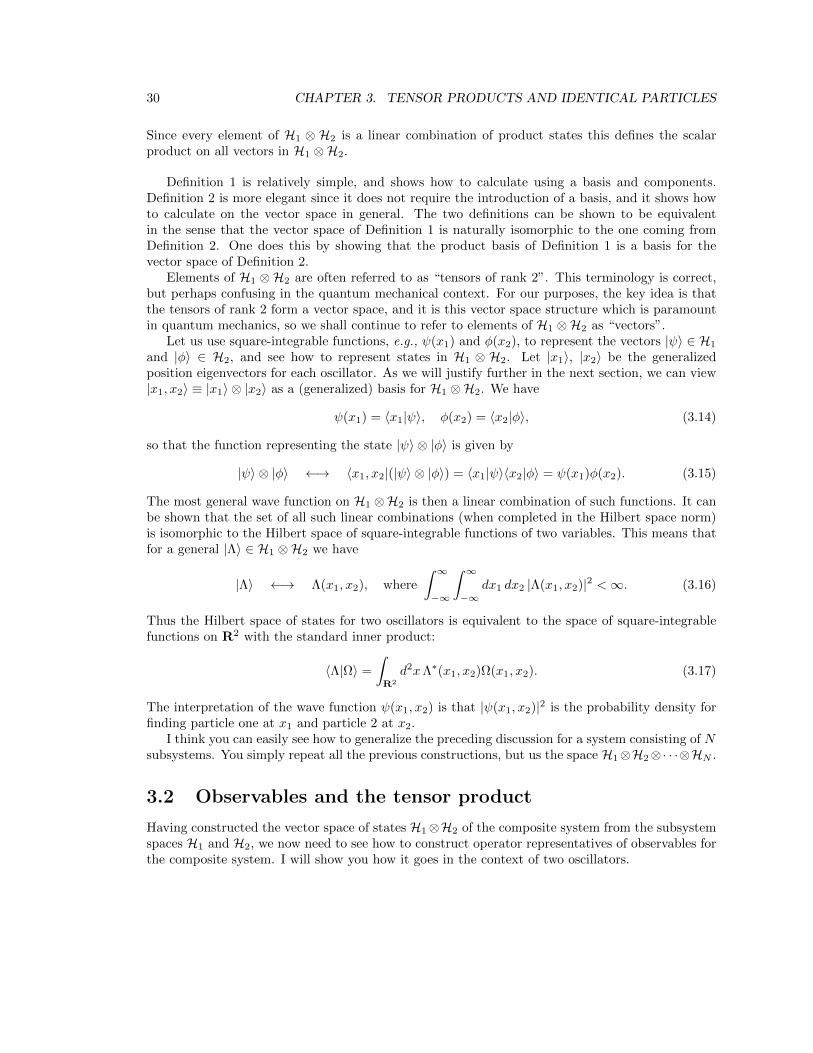
Definition 1 is relatively simple, and shows how to calculate using a basis and components.Definition 2 is more elegant since it does not require the introduction of a basis, and it shows howto calculate on the vector space in general. The two definitions can be shown to be equivalentin the sense that the vector space of Definition 1 is naturally isomorphic to the one coming fromDefinition 2. One does this by showing that the product basis of Definition 1 is a basis for thevector space of Definition 2.
Elements of H1 ⊗H2 are often referred to as “tensors of rank 2”. This terminology is correct,but perhaps confusing in the quantum mechanical context. For our purposes, the key idea is thatthe tensors of rank 2 form a vector space, and it is this vector space structure which is paramountin quantum mechanics, so we shall continue to refer to elements of H1 ⊗H2 as “vectors”.
Let us use square-integrable functions, e.g., ψ(x1) and φ(x2), to represent the vectors |ψ〉 ∈ H1
and |φ〉 ∈ H2, and see how to represent states in H1 ⊗ H2. Let |x1〉, |x2〉 be the generalizedposition eigenvectors for each oscillator. As we will justify further in the next section, we can view|x1, x2〉 ≡ |x1〉 ⊗ |x2〉 as a (generalized) basis for H1 ⊗H2. We have
ψ(x1) = 〈x1|ψ〉, φ(x2) = 〈x2|φ〉, (3.14)
so that the function representing the state |ψ〉 ⊗ |φ〉 is given by
|ψ〉 ⊗ |φ〉 ←→ 〈x1, x2|(|ψ〉 ⊗ |φ〉) = 〈x1|ψ〉〈x2|φ〉 = ψ(x1)φ(x2). (3.15)
The most general wave function on H1 ⊗H2 is then a linear combination of such functions. It canbe shown that the set of all such linear combinations (when completed in the Hilbert space norm)is isomorphic to the Hilbert space of square-integrable functions of two variables. This means thatfor a general |Λ〉 ∈ H1 ⊗H2 we have
|Λ〉 ←→ Λ(x1, x2), where
∫ ∞−∞
∫ ∞−∞
dx1 dx2 |Λ(x1, x2)|2 <∞. (3.16)
Thus the Hilbert space of states for two oscillators is equivalent to the space of square-integrablefunctions on R2 with the standard inner product:
〈Λ|Ω〉 =
∫R2
d2xΛ∗(x1, x2)Ω(x1, x2). (3.17)
The interpretation of the wave function ψ(x1, x2) is that |ψ(x1, x2)|2 is the probability density forfinding particle one at x1 and particle 2 at x2.
I think you can easily see how to generalize the preceding discussion for a system consisting of Nsubsystems. You simply repeat all the previous constructions, but us the space H1⊗H2⊗· · ·⊗HN .
3.2 Observables and the tensor product
Having constructed the vector space of states H1⊗H2 of the composite system from the subsystemspaces H1 and H2, we now need to see how to construct operator representatives of observables forthe composite system. I will show you how it goes in the context of two oscillators.

3.2. OBSERVABLES AND THE TENSOR PRODUCT 31
Each oscillator has its respective observables, represented by linear operators constructed from(x1, p1) and (x2, p2). Our first task is to see how these subsystem observables are represented onthe vector space of states for the composite system. Given a basis |i〉, i = 1, 2, . . . , for a singleoscillator (e.g., the basis of energy eigenvectors) any state vector |Ψ〉 ∈ H1 ⊗H2 can be expandedin a product basis:
|Ψ〉 =∑i,j
Ψij |i〉 ⊗ |j〉. (3.18)
Let A1 be an operator defined on H1. We extend its definition to |Ψ〉 ∈ H1 ⊗H2 via
A|Ψ〉 =∑i,j
Ψij (A1|i〉)⊗ |j〉. (3.19)
Similarly if B2 is an operator defined on H2 we extend its definition to |Ψ〉 ∈ H1 ⊗H2 via
B|Ψ〉 =∑i,j
Ψij |i〉 ⊗ (B2|j〉). (3.20)
The extension of A1 and B2 to |Ψ〉 ∈ H1 ⊗H2 uses the pretty obvious notation
A = A1 ⊗ 1, B = 1⊗ B2. (3.21)
With this definition you can see that a pair of observables A1 and B2 for systems 1 and 2 willhave a product given by A1 ⊗ B2 and that they will always be compatible, that is, their operatorrepresentatives will commute:
[A, B] = (A1 ⊗ 1)(1⊗ B2)− (1⊗ B2)(A1 ⊗ 1) = A1 ⊗ B2 − A1 ⊗ B2 = 0. (3.22)
It follows that the positions, momenta, energies etc. for each oscillator will be compatible andone may use any two bases of eigenvectors to span the Hilbert space of the composite system. Forexample one can use position eigenvectors: |x1〉 ⊗ |x2〉, or position and momentum eigenvectors|x1〉 ⊗ |p2〉 or energy eigenvectors |E1〉 ⊗ |E2〉, and so forth. Such bases represent states in whichthe respective observables for each particle are known with statistical certainty.
Besides the usual observables pertaining to subsystems, new observables for the compositesystem are also available. For example, the total energy of the system is defined as
H = H1 ⊗ 1 + 1⊗ H2. (3.23)
Eigenvectors for this operator are in fact just the product of energy eigenvectors for the subsystem:
H|Em〉 ⊗ |En〉 = (H1|Em〉)⊗ |En〉+ |Em〉 ⊗ (H2|En〉)= Em|Em〉 ⊗ |En〉+ En|Em〉 ⊗ |En〉= (Em + En)|Em〉 ⊗ |En〉. (3.24)
Physically, these product vectors are states in which the individual energies and the total energyare known with certainty. A basis of such states is available because the three relevant operatorscommute.
32 CHAPTER 3. TENSOR PRODUCTS AND IDENTICAL PARTICLES
I think you can easily see how to generalize the preceding discussion for a system consisting of Nsubsystems. You simply repeat all the previous constructions, but use the space H1⊗H2⊗· · ·⊗HN .Observables pertaining to, say, subsystem k would take the form
1⊗ 1⊗ · · · 1⊗ Ak ⊗ 1 · · · ⊗ 1. (3.25)
This Hilbert space and operators on it would be the setting for the quantum theory of a dynamicalsystem near stable equilibrium if each of the component Hilbert spaces were that of a quantumoscillator, i.e., square-integrable functions of one variable. In this way one gets the quantum theoryof normal modes of vibration for a mechanical system. As we shall see in the next chapter, if weconsider a limit in which N become arbitrarily large we get one way of thinking about a quantumfield.
3.3 Symmetric and antisymmetric tensors. Identical parti-cles.
Recall that identical particles are those which are intrinsically alike, in the sense that they all sharecertain observable characteristics – their defining properties – although they can differ in otherobservable regards. So, for example, all electrons have the same mass, electric charge, spin, and soforth, although they can be in different locations, have different velocities, and have different spinstates. Consider a system of such identical particles. If the roles of two particles are interchangedin the composite system, the state of the system should be unchanged. Since the state of such asystem must not distinguish any particular particle, there is a new postulate of quantum mechanicswhich applies to identical particles. It involves the symmetric and antisymmetric tensor product,which I will now explain.
Identical particles have identical Hilbert spaces of state vectors. Let us consider two identicalparticles and their respective Hilbert spaces H1 and H2. The system of two particles is describedby the Hilbert space H1⊗H2, but we must take account of the indistinguishability of the particles.Consider a product vector |α〉 ⊗ |β〉 ∈ H1 ⊗ H2. We can decompose it into its symmetric andantisymmetric parts:
|α〉 ⊗ |β〉 =1
2(|α〉 ⊗ |β〉+ |β〉 ⊗ |α〉) +
1
2(|α〉 ⊗ |β〉 − |β〉 ⊗ |α〉)
≡ |α, β〉s + |α, β〉a. (3.26)
The symmetric vectors do not change when the roles of the particles are interchanged. The anti-symmetric vectors change by a sign when the roles of the particles are interchanged. A sign changeis a phase factor; as mentioned back in the postulates any two vectors which differ by a phase factordefine the same state. Thus either possibility is permissible when considering identical particles.
The decomposition (3.26) can be extended to each term in the expansion of a vector in a productbasis, so we can partition H1 ⊗H2 into its symmetric part [H1 ⊗H2]s and its antisymmetric part[H1 ⊗H2]a. Each of these subspaces is a Hilbert space.
For composite systems consisting of more than two particles, one can still consider the subspaceof vectors which are unchanged under particle permutation (“symmetric”), or change sign underpermutation (“antisymmetric”). Unlike the case with just two particles, these two subspaces do notexhaust the whole vector space – there are states with intermediate “Young tableaux symmetries”.So far, it appears that nature does not take advantage of this latter type of state vector symmetry.

3.3. SYMMETRIC AND ANTISYMMETRIC TENSORS. IDENTICAL PARTICLES. 33
We are now ready to add a new quantum mechanics postulate: The states for identical quantumsystems are given by either the symmetric or antisymmetric subspace of the tensor product.
You may recall that in statistical thermodynamics identical particles described by symmetricstates obey Bose-Einstein statistics and are called “bosons” while those described by the antisym-metric states obey Fermi-Dirac statistics and are called “fermions”. It is a theorem of relativisticquantum field theory that integral spin particles are bosons and half-integral spin particles arefermions. We will explore this fact just a little when we finally get around to constructing photons,which have spin-1. Whether a particle is a boson or a fermion is one of those intrinsic features thatmakes the particle what it is.3
The number of states available to a system of particles depends strongly on whether or not theyare identical, and, if they are identical, whether or not they are bosons or fermions. Given twosingle particle states |α〉, |β〉, there is a two-dimensional space of physically inequivalent states onecan make for a system consisting of 2 distinguishable particles:4
|Ψ〉distinguishable = a|α〉 ⊗ |β〉+ b|β〉 ⊗ |α〉, |a|2 + |b|2 = 1. (3.27)
In this family of states |a|2 is the probability for finding particle 1 in state |α〉 and particle 2 instate |β〉, while |b|2 is the probability for finding particle 1 in state |β〉 and particle 2 in state |α〉.In light of the new quantum postulate for identical particles, there is only one way to construct astate of identical particles from the given 1-particle states:
|Ψ〉identical =1√2
(|α〉 ⊗ |β〉 ± |β〉 ⊗ |α〉) , (3.28)
where the plus/minus sign goes with bosons/fermions. This is a state in which one particle is inthe state |α〉 and one particle is in the state |β〉. Moreover, if the particles are identical fermionsthen they cannot be in the same state, |α〉 6= |β〉 – this is the quantum mechanical implementationof the Pauli exclusion principle.
This new quantum postulate for systems composed of identical subsystems puts limitations onthe allowed observables since not every operator restricts to act on the symmetric or antisymmet-ric subspace. Let us consider a simple example. For two distinct oscillators, each in an energyeigenstate, one has a state described by the vector
|Ψ〉 = |n〉 ⊗ |j〉, (3.29)
in which the first oscillator has energy (n+ 12 )~ω1 with statistical certainty and the second oscillator
has energy (j + 12 )~ω2 with certainty. If we want to model this situation for identical oscillators we
should set m1 = m2 ≡ m and ω1 = ω2 = ω and then restrict to symmetric or antisymmetric states:
|Ψ〉 =1√2
|n〉 ⊗ |j〉+ |j〉 ⊗ |n〉
, bosons, (3.30)
|Ψ〉 =1√2
|n〉 ⊗ |j〉 − |j〉 ⊗ |n〉
, fermions. (3.31)
3Here it might be good to mention that in supersymmetric theories the distinction between bosons and fermionsis not so clear-cut!
4There are two complex constants, so a priori there four real parameters. Normalization fixes one real parameter,and the equivalence of any two vectors if they differ by a phase removes another real parameter.
34 CHAPTER 3. TENSOR PRODUCTS AND IDENTICAL PARTICLES
The meaning of the state now is that one of the oscillators has energy (n+ 12 )~ω and the other has
energy (j+ 12 )~ω. If the oscillators are identical, by definition there is no way to tell which is which
and this sort of description of, say, an energy eigenstate is the best one can do. Indeed, there canbe no observables which pertain to this or that particle individually since they are all identical. Forexample, the operator representing energy of oscillator 1, H ⊗ 1 is no longer well-defined since itdoes not map the symmetric or antisymmetric subspace into itself:
(H ⊗ 1)|Ψ〉 =1√2
(n+
1
2)~ω|n〉 ⊗ |j〉 ± (j +
1
2)~ω|j〉 ⊗ |n〉
. (3.32)
To interchange the roles of the oscillators in (3.32) you replace |n〉 ⊗ |j〉 ↔ |j〉 ⊗ |n〉 and you willsee that the state vector does not stay the same (up to a sign) when n 6= j.
There are, of course, observables which can be used to describe a system comprised of identicalsubsystems. For example, the total energy of the system,
Htotal = H ⊗ 1 + 1⊗ H, (3.33)
is a well-defined operator on the symmetric and antisymmetric subspaces. For example, you cancheck that the product state we just considered is an eigenvector:
Htotal|Ψ〉 =
[(n+
1
2)~ω + (j +
1
2)~ω
]1√2
|n〉 ⊗ |j〉 ± |j〉 ⊗ |n〉
= (n+ j + 1)~ω|Ψ〉. (3.34)
Evidently this state is one in which the energy is (n+j+1)~ω with statistical certainty. Since thesesymmetrized product vectors span the Hilbert space for this identical system of identical particlesthe operator Htotal is well-defined. It is not too hard to show that an operator is well-defined onthe symmetric or anti-symmetric subspace of states if and only if it is invariant under interchangeof the roles of the particles.
3.4 Symmetrization and anti-symmetrization for any num-ber of particles
It is worth briefly describing how one builds the symmetric and antisymmetric state vectors forsystems consisting of more than two (identical) subsystems. To begin, let us consider a productstate of 3 harmonic oscillators; let the states be represented energy eigenvectors:
|Ψ〉 = |n1〉 ⊗ |n2〉 ⊗ |n3〉. (3.35)
This state could apply to a system of of 3 distinguishable oscillators each of which has, withprobability one, energy (n1 + 1
2 )~ω1, (n2 + 12 )~ω2, (n1 + 1
2 )~ω3. To make the oscillators “identical”,set ω1 = ω2 = ω3 and m1 = m2 = m3. The totally symmetric and antisymmetric parts of this stateare given by
|Ψ〉s =1√3!
|n1〉 ⊗ |n2〉 ⊗ |n3〉+ |n2〉 ⊗ |n3〉 ⊗ |n1〉+ |n3〉 ⊗ |n1〉 ⊗ |n2〉
+(|n1〉 ⊗ |n3〉 ⊗ |n2〉+ |n2〉 ⊗ |n1〉 ⊗ |n3〉+ |n3〉 ⊗ |n2〉 ⊗ |n1〉
)(3.36)
3.5. PROBLEMS 35
|Ψ〉a =1√3!
|n1〉 ⊗ |n2〉 ⊗ |n3〉+ |n2〉 ⊗ |n3〉 ⊗ |n1〉+ |n3〉 ⊗ |n1〉 ⊗ |n2〉
−(|n1〉 ⊗ |n3〉 ⊗ |n2〉+ |n2〉 ⊗ |n1〉 ⊗ |n3〉+ |n3〉 ⊗ |n2〉 ⊗ |n1〉
)(3.37)
In the symmetric case I summed over all permutations – the first three terms involve the “even”permutations, which involve an even number of interchanges, and the second three terms involvethe “odd” permutations, which involve an odd number of interchanges. In the antisymmetric caseI subtracted the sum over odd permutations from the sum over even permutations. These stateswould describe energy eigenstates of three identical bosons and fermions, respectively.
Given three distinct 1-particle energy eigenstates, there are 3! = 6 possible ways to assignparticles to those states. So, in the case where all three particles were somehow distinguishablethere would be 6 product states for the composite system which I could construct from the three1-particle energy eigenstates. If the particles are indistinguishable there is only one state available!
In general, the symmetric and antisymmetric parts of a product state of p particles are given by
|Ψ〉 = |n1〉 ⊗ |n2〉 ⊗ · · · ⊗ |np〉, (3.38)
|Ψ〉s =1√p!
∑even
permutations
|n1〉 ⊗ |n2〉 ⊗ · · · ⊗ |np〉+∑odd
permutations
|n1〉 ⊗ |n2〉 ⊗ · · · ⊗ |np〉
, (3.39)
|Ψ〉a =1√p!
∑even
permutations
|n1〉 ⊗ |n2〉 ⊗ · · · ⊗ |np〉 −∑odd
permutations
|n1〉 ⊗ |n2〉 ⊗ · · · ⊗ |np〉
, (3.40)
The symmetric or anti-symmetric subspaces of the Hilbert space of states are obtained by consid-ering linear combinations of states (3.39) or (3.40), respectively.
3.5 Problems
1. Construct the Schrodinger equation for two harmonic oscillators characterized by masses m1,m2 and frequencies ω1, ω2. Find/describe its general solution. Notice that the wave functiondefines waves in R2 rather than two waves in R1.
2. Consider two identical oscillators, one in a state represented by the position wave function ψ1,one in a state represented by the wave function ψ2. Construct the position wave function ofthe composite system in the case of distinguishable particles, in the case of bosons, and in thecase of fermions. For each case compute the probability density that an oscillator is at x1 andthe other oscillator is at x2. Show that in the case of bosons the probability is enhanced forthe particles to be near each other compared to the distinguishable case, while the probabilityis reduced in the case of fermions. Finally, show that this effect becomes negligible if theparticles are sufficiently localized away from each other in the sense that the overlap of thesupports of the two 1-particle wave functions is negligible.
36 CHAPTER 3. TENSOR PRODUCTS AND IDENTICAL PARTICLES
3. ConsiderN fermionic oscillators in 1-particle states, represented by wave functions ψ1, ψ2, . . . , ψN .Show that the wave function of the composite system can be represented by the Slater deter-minant
Ψ(x1, x2, . . . , xN ) =1√N !
det
ψ1(x1) ψ2(x1) . . . ψN (x1)ψ1(x2) ψ2(x2) . . . ψN (x2)
. . . .
. . . .
. . . .ψ1(xN ) ψ2(xN ) . . . ψN (xN )
.
Under what circumstances will this wave function be identically zero? (If your muscles arenot strong enough, you can restrict your answer to the case N = 3.)
4. Show that a well-defined operator for a system of identical bosons or fermions must be invari-ant under any interchange of two particles.
5. A particle has a two-dimensional Hilbert space with orthonormal basis |1〉, |2〉. Consider asystem consisting of two such particles, assumed distinguishable. Set up the Hilbert spaceof the composite system using both definitions and indicate how vectors in each versioncorrespond. Show that in each definition the product basis induced by |1〉, |2〉 is orthonormal.
6. Show that the Hamiltonian (3.33) is a well-defined operator on the symmetric and anti-symmetric subspaces of the Hilbert space. This means you should show that Htotal mapssymmetric states to symmetric states and anti-symmetric states to anti-symmetric states.
7. A (non-relativistic) particle with spin- 12 is characterized by a trio of linear operators on the2-d Hilbert space C2 representing components of the spin vector ~s:
sx =~2
(0 11 0
), sy =
~2
(0 −ii 0
), sz =
~2
(1 00 −1
).
Consider two distinguishable spin- 12 particles. Construct the individual spin operators, ~S1 and~S2 as matrices on the 4-dimensional space C4 = C2⊗C2 in the product basis of eigenvectorsof S1z and S2z. Construct the matrix representing the total spin, ~S = ~S1 + ~S2 again in theproduct basis of eigenvectors of S1z and S2z. How should ~S be represented if the particles areidentical?
8. For a system of two identical harmonic oscillators, show that while the individual momentaare not well-defined observables the total momentum is well-defined.
9. Consider two particles, for simplicity moving in one dimension. Construct the operatorsrepresenting the center of mass X, the total momentum P , the relative position x, and therelative momentum p, all in terms of the individual position and momentum operators (x1, x2)and (p1, p2). Construct a (generalized) eigenfunction of x and P with eigenvalues a and 0respectively, corresponding to the particles having zero total momentum and a statisticallycertain separation a.
(Why this is an interesting problem: In this state, suppose that particle 2’s momentum ismeasured to have the value p2. Then particle 1 has momentum −p2 with statistical certainty

3.5. PROBLEMS 37
and its position is completely uncertain. Suppose instead that particle 2’s position is measuredand found to have the value x2. Then particle 1’s position is known with certainty to have thevalue x2−a and its momentum is completely uncertain. Thus measurements made on particle2 appear to affect the outcome of measurements made on particle 1. This is the essence ofthe Einstein-Podolsky-Rosen paradox [4].)
10. What is the ground state and ground state energy of a system consisting of three non-interacting oscillators if they are all distinguishable. What if the particles are identical bosons?How about identical fermions?
11. You know that the states of motion of a particle in three dimensions can be represented by awave function ψ(~x). You also know that the spin states of a spin- 12 system can be representedby a column vector χ with two complex entries. Using tensor product constructions, explainhow states of a spin- 12 particle moving in 3-d should be represented.
12. For any physical system, the operators representing angular momentum are a trio ~J =(Jx, Jy, Jz) satisfying
[Ja, Jb] = i~εabcJc, (3.41)
where εabc is the Levi-Civita permutation symbol. Define the length-squared of angular mo-mentum by the operator
J2 = J2x + J2
y + J2z .
Using (3.41), show that [Ja, J2] = 0 for any a = x, y, z. Consider a composite system con-
sisting of two systems with angular momenta ~J1 and ~J2 acting on Hilbert spaces H1 and H2.Define the total angular momentum of the system in the usual way by
~J = ~J1 ⊗ 1 + 1⊗ ~J2.
Show that the total angular momentum ~J satisfies (3.41). Show that
[J2, J1a] 6= 0, [J2, J2a] 6= 0,
so that states of definite total angular momentum will not necessarily be states of definiteindividual angular momentum.
Chapter 4
Fock Space
In quantum mechanics one considers systems consisting of a fixed number of particles. If there areN particles, the N -fold tensor product of the 1-particle Hilbert spaces suffices to define the states.Particle observables are represented as operators on the tensor product. In quantum field theorywe consider systems where the number of particles in the system is variable. How to build a Hilbertspace of states and operator observables which allows this? Fock space.
4.1 Definitions
Fock space F is canonically defined from any given Hilbert space H using direct sums and tensorproducts.(I will use the Hilbert space H of square integrable functions on the real line, suitable forthe harmonic oscillator, as a running example.) In this context H is called the 1-particle Hilbertspace; it represents the set of states of a single particle, e.g., an oscillator. As we have seen thespace H ⊗ H can be viewed either as the set of states for a single particle in higher dimensions,or as the set of states of two particles. Let’s use the latter interpretation, and let us assume theparticles are identical so we only work with the symmetric or antisymmetric subspace accordingto whether the particles are bosons or fermions. Similarly we can view H ⊗ H ⊗ H as the spaceof states of 3 particles; if the particles are identical we again take the symmetric or antisymmetricsubspace. As you can imagine, we can keep on building Hilbert spaces of states for any numberof identical particles by taking the appropriate number of tensor products and then taking theappropriate symmetric or antisymmetric subspace. Fock space is defined as the direct sum of theset of complex numbers C (viewed as a 1-d Hilbert space) with the one particle Hilbert space, withthe two particle Hilbert space, with the three particle Hilbert space, and so forth.1 Before seeinghow that all works in detail, let me make sure you are comfortable with the notion of the directsum of two vector spaces.
Given two vector spaces V1 and V2 of dimension, say, n1 and n2, the direct sum of V1 and V2 isthe vector space V = V1⊕V2 of dimension n1 +n2 obtained by taking the Cartesian product of thetwo vector spaces. An element |w〉 ∈ V1 ⊕ V2 is then an ordered pair (|w1〉, |w2〉) where |w1〉 ∈ V1
1Technically, the Fock space is defined as the completion of this direct sum of tensor products using the norminduced by the scalar product, which will be defined shortly.
38

4.1. DEFINITIONS 39
and |w2〉 ∈ V2. If you like to think in terms of column vectors, we could write
|w1〉 =
a1a2...an1
, |w2〉 =
b1b2...bn2
, |w〉 =
a1a2...an1
b1b2...bn2
, (4.1)
As a familiar example, the usual x-y-z vector space R3 can be written as a direct sum in a coupleof ways: R3 = R⊕R2 = R⊕R⊕R.
Addition and scalar multiplication on V = V1 ⊕ V2 are defined by
|w〉+ |u〉 = (|w1〉+ |u1〉, |w2〉+ |u2〉), c|w〉 = (c|w1〉, c|w2〉), (4.2)
this endows V1 ⊕ V2 with the structure of a (complex) vector space. The scalar product used toprovide the Hilbert space structure is defined via
〈w|u〉 = 〈w1|u1〉+ 〈w2|u2〉. (4.3)
You can check that all this vector space structure is just the usual one for the set of column vectors(4.1).
Let us denote the Hilbert space of complex numbers by C ≡ H0, the one particle Hilbert spacecan be denoted by H ≡ H1, the two particle Hilbert space can be denoted by H2 ≡ H⊗H, where arestriction to the symmetric or antisymmetric subspace is tacitly assumed, and so forth. The Fockspace F is the Hilbert space defined by2
F = H0 ⊕H1 ⊕H2 ⊕H3 ⊕ · · · . (4.4)
The direct sums go on forever! What can that mean?Let us start by focusing on the harmonic oscillator example. An element of C is just a complex
number, say, ψ0. An element of H1 is a square-integrable function ψ1(x1). An element of H2
is a square-integrable function of two variables ψ(x1, x2) satisfying either ψ(x1, x2) = ψ(x2, x1)or ψ(x1, x2) = −ψ(x2, x1), depending upon whether we are dealing with bosons or fermions. Anelement of H3 is a square-integrable function of 3 variables, ψ(x1, x2, x3) which is symmetric orantisymmetric under any permutation of its arguments. In this way an element |Ψ〉 ∈ F is aninfinite sequence:
|Ψ〉 = (ψ0, ψ1(x1), ψ2(x1, x2), . . . , ψn(x1, x2, . . . , xn), . . . ). (4.5)
The scalar product of |Ψ〉 and |Φ〉,
|Φ〉 = (φ0, φ1(x1), φ2(x1, x2), . . . , φn(x1, x2, . . . , xn), . . . ) (4.6)
2Again, we should form the completion of this vector space using the norm induced by the scalar product.
40 CHAPTER 4. FOCK SPACE
is an infinite series:
〈Ψ|Φ〉 = ψ∗0φ0 +
∫ ∞−∞
dx1 ψ∗1(x1)φ1(x1) +
∫ ∞−∞
dx1
∫ ∞−∞
dx2 ψ∗2(x1, x2)φ2(x1, x2) + · · · (4.7)
We require that this series converges. This is guaranteed if
〈Ψ|Ψ〉 = |ψ0|2 +
∫ ∞−∞
dx1 |ψ1(x1)|2 +
∫ ∞−∞
dx1
∫ ∞−∞
dx2 |ψ2(x1, x2)|2 + · · · <∞ (4.8)
Evidently, the Hilbert space norm of the functions ψn(x1, x2, . . . , xn) must vanish as n → ∞.Vectors in F representing states of a quantum system will be normalized, 〈Ψ|Ψ〉 = 1.
At this point it is worth previewing the physical interpretation of the Fock state just described.(I will explain how this interpretation arises in a little while.) In the state represented by |Ψ〉, |ψ0|2is the probability that there are no particles present; |ψ(x1)|2 is the probability density that oneparticle is present at a displacement x1; |ψ(x1, x2)|2 is the probability density that two particles arepresent at the displacements x1 and x2; ψn(x1, x2, . . . , xn)|2 is the probability density for findingn particles at displacements x1, x2, . . . , xn. The Hilbert space norms of each of the wave functionsappearing in (4.8) are then the probabilities for finding 0, 1, 2, . . . , n, . . . particles, respectively inthe state |Ψ〉. Now you can see how Fock space is the setting for considering systems where thenumber of particles can vary. It is interesting to note that, statistically speaking, the states |Ψ〉need not have a definite number of particles!
4.2 Occupation numbers. Creation and annihilation opera-tors.
I now want to introduce some fundamental tools for working with the Fock space. We begin byfocusing on the example of identical harmonic oscillators. Let us use the basis of energy eigenvectors,|n〉 ≡ |En〉, n = 0, 1, 2, . . . , for the Hilbert space of one oscillator to induce a basis on F . An obviousbasis we can make is of the form
|β〉 =(z, |a〉, |b〉 ⊗ |c〉, |d〉 ⊗ |e〉 ⊗ |f〉, . . .
), z ∈ C, a, b, c, d, e, f, · · · = 0, 1, 2, 3, . . . , (4.9)
where I will leave implicit the symmetrization or anti-symmetrization of each element of the se-quence. This basis is just fine, but there is a more useful choice we can make. For each choice ofa, b, c, . . . the basis vector |β〉 can itself be viewed as a linear combination of a zero particle state,a 1-particle state, a 2-particle state, and so forth:
|β〉 =(
1, 0, 0, . . .)
+(
0, |a〉, 0, 0, . . .)
+(
0, 0, |b〉 ⊗ |c〉, . . .)
+ . . . (4.10)
Again, symmetrization or anti-symmetrization is implicit. Evidently, we can view our basis asconsisting of the following: a state with 0 particles – the vacuum state; all states with 1 particlein the various energy eigenstates; all states with two particles in the various energy eigenstates,and so forth. Each element of this basis has a fixed number of particles, say p. We can uniquelyspecify a basis element with p particles by simply specifying how many of the p particles are in theground state, how many are in the first excited state, and so on. These are the occupation numbers.For bosons the occupation numbers can be any non-negative integers. For fermions the occupation

4.2. OCCUPATION NUMBERS. CREATION AND ANNIHILATION OPERATORS. 41
numbers can only be 0 or 1. The resulting basis for F is called the occupation number basis. Anoccupation number basis vector describing p particles, with n0 in the ground state, with n1 in thefirst excited state, and so forth is denoted by
|n0, n1, n2, . . .〉, n0 + n1 + n2 + · · · = p. (4.11)
The vacuum state, with no particles present, is usually denoted by |0〉. Given the energy eigenvectorbasis (or any other basis we wish to use) for the one particle Hilbert space, the occupation numberbasis vectors are labeled by an infinite sequence of occupation numbers. The occupation basis isorthonormal.
Two linear operators on F which are of fundamental utility are the creation and annihilationoperators, denoted by a†k and ak, respectively, where k = 0, 1, 2, . . . . These operators add orremove a particle in the energy eigenstate labeled by the non-negative integer k. To define anylinear operator mathematically it suffices to give its action on a basis; here are the definitions of a†kand ak via the occupation number basis.
Bosonsak|n0, n1, . . . nk, . . .〉 =
√nk|n0, n1, . . . nk − 1, . . .〉, (4.12)
a†k =√nk + 1|n0, n1, . . . nk + 1, . . .〉. (4.13)
Fermions
ak|n0, n1, . . . nk = 0, . . .〉 = 0, ak|n0, n1, . . . nk = 1, . . .〉 = (−1)α(k)|n0, n1, . . . nk = 0, . . .〉 (4.14)
a†k|n0, n1, . . . nk = 0, . . .〉 = (−1)α(k)|n0, n1, . . . nk = 1, . . .〉, a†k|n0, n1, . . . nk = 1, . . .〉 = 0, (4.15)
where (−1)α is ±1 according to whether the number of occupied 1-particle states lower than k iseven/odd. You can check that this rule is satisfied for identical harmonic oscillators if we set
α(k) = n0 + n1 + · · ·+ nk−1. (4.16)
In both the boson and fermion cases the result of applying an operator is the zero vector (notthe vacuum vector!) if a negative occupation number were to occur. Let us spend a little timeunderstanding the ramifications of all these definitions.
It is straightforward to apply the definitions given above to verify the following fundamentalresults.
• The creation and annihilation operators are related by Hermitian conjugation:
a†k = (ak)†. (4.17)
• The bosonic operators satisfy the following commutation relations:
[ak, al] = [a†k, a†l ] = 0, [ak, a
†l ] = δkl1, (4.18)
where the commutator is defined as [A, B] ≡ AB − BA.

42 CHAPTER 4. FOCK SPACE
• The fermionic operators satisfy the following anti-commutation relations:
ak, al = a†k, a†l = 0, ak, a†l = δkl1, (4.19)
where the anti-commutator is defined as A, B ≡ AB+BA. Note in particular that a†ka†k = 0,
so the occupation number of a given state is 0 or 1, which is again the Pauli exclusion principle.
• For both bosons and fermions, the number operator Nk for the 1-particle state labeled by k,defined by
Nk = a†kak, (4.20)
acts on the occupation number basis via
Nk|n0, n1, . . . nk, . . .〉 = nk|n0, n1, . . . nk, . . .〉. (4.21)
The occupation number basis vectors are eigenvectors of Nk. Evidently, the operator N representingthe total number of particles is
N =∑k
Nk. (4.22)
Each of the n-fold tensor product vectors appearing in the superposition (4.10) is an eigenvectorof N with eigenvalue n. Therefore, as advertised earlier, the wave functions of the form ψ(x1, . . . , xn)appearing in (4.5) are position probability amplitudes for states with n particles.
As mentioned earlier, the state with no particles is the vacuum state, usually denoted |0〉 (notthe zero vector!). It satisfies
ak|0〉 = 0, ∀ k, (4.23)
and this can be taken to be its definition. A state with a single particle in the one particle state|k〉 is
|0, . . . , nk = 1, 0, . . .〉 = a†k|0〉 (4.24)
If we add a particle to, say, energy state m < k, we get the state
|0, . . . , nm = 1, . . . , nk = 1, 0, . . .〉 = a†ma†k|0〉 (4.25)
if we add the particles in the reverse order we get the same vector for bosons and (−1) timesthe vector in the case of fermions. This implements the convention that the 1-particle states in amulti-particle fermion state are the anti-symmetrization of a state which is in increasing order withrespect to energy. A basis for the N -particle subspace of F is obtained from the vectors
a†k1a†k2· · · a†kN |0〉, ∀ k1, k2, . . . , kN . (4.26)
The union of these bases for each N defines a basis for F . A state vector is any normalized linearcombination of these occupation number basis vectors. As such, I remind you that states neednot be eigenvectors of Nk or even N . The number of particles in a state is subject to statisticalfluctuations!
Although I have not done it here, one can develop the preceding results in a way which showsthat Fock space can be defined as a vector space representing the algebra of creation and annihilationoperators (4.17)–(4.19). Roughly speaking, once the commutation (or anti-commutaiton relations)are specified, the Fock space is determined. Here I have simply built the Fock space, postulatedthe form of the creation and annihilation operators, and deduced some of their properties. For asystematic derivation of creation and annihilation operator formulas see, for example, [2].

4.3. OBSERVABLES. FIELD OPERATORS. 43
4.3 Observables. Field operators.
Here we will explore the construction of operators on F representing observables of a system witha variable number of particles.
4.3.1 1-particle observables
The simplest observables are the “additive 1-particle” observables, which arise by taking a propertywhich can be assigned to each individual particle and summing it over all particles in the system.We have already seen an example of such an operator: the number operator N . In our oscillatorexample, we can of course measure an energy for each oscillator; the total energy is obtained bysumming the result. The operator which represents this observable is
H =∑k
Ek Nk, (4.27)
where Ek = (k+ 12 )~ω. The occupation number basis we have been using is also the basis of energy
eigenvectors:
H|n0, n1, n2, . . .〉 =
(∑k
nkEk
)|n0, n1, n2, . . .〉. (4.28)
This is possible since [H, Nk] = 0.The total energy was easy to define since we chose to work in the occupation number basis
associated to 1-particle energy eigenstates. To construct operators for other additive 1-particleobservables we use a similar strategy: use the basis of eigenvectors of the chosen 1-particle operatorto build the Fock basis. For example, let’s build the total momentum of the system. We can usethe basis of 1-particle momentum eigenvectors |p〉 to build an occupation number basis for the Fockspace. This entails using integrals instead of sums over the basis, and we must be careful to keepin mind that this basis is of the “generalized” type.
Recall that, for one particle, the bases of energy eigenvectors |Ek〉 and momentum eigenvectors|p〉 are related by
|Ek〉 =
∫ ∞−∞
dp uk(p)|p〉, |p〉 =∑k
u∗k(p)|Ek〉, (4.29)
where uk(p) is the momentum space energy eigenfunction
uk(p) = 〈p|Ek〉. (4.30)
Using these relations, let us define the creation and annihilation operators for particles with mo-mentum p to be a†(p) and a(p):
a†(p) =∑l
u∗l (p)a†l (4.31)
anda(p) =
∑l
ul(p)al (4.32)
The bosonic creation and annihilation operators satisfy the following commutation relations:
[a(p), a(p′)] = [a†(p), a†(p′)] = 0, [a(p), a†(p)] = δ(p, p′)1. (4.33)

44 CHAPTER 4. FOCK SPACE
The fermionic operators satisfy the following anti-commutation relations:
a(p), a(p′) = a†(p), a†(p′) = 0, a(p), a†(p) = δ(p, p′)1. (4.34)
In terms of our original basis (4.9) for F , we have
a†(p)(1, 0, 0, . . . ) =∑k
u∗k(p)a†k(1, 0, 0, . . . ) = (0,∑k
u∗k(p)|Ek〉, 0, . . . ) = (0, |p〉, 0, . . .〉 (4.35)
and
a†(p2)(0, |p1〉, 0, . . . ) = a†(p2)(0,∑k
u∗k(p1)|Ek〉, 0, . . . ) (4.36)
= (0, 0,∑k,l
u∗k(p1)u∗l (p2)(0, 0,1√2
[|Ek〉 ⊗ |El〉 ± |El〉 ⊗ |Ek〉] , 0, . . . ) (4.37)
= (0, 0,1√2
(|p1〉 ⊗ |p2〉 ± |p2〉 ⊗ |p1〉), 0, . . . ). (4.38)
In this way we can build a basis for the Fock space from the 1-particle basis of momentum eigen-vectors.
Using the same logic as with the energy, the total momentum operator is defined to be
P =
∫ ∞−∞
dp p a†(p)a(p). (4.39)
Using (4.31), (4.32), the total momentum operator can be written in terms of the energy basis as
P =
∫ ∞−∞
dp p∑k,l
u∗k(p)ul(p)a†kal (4.40)
This expression of P in the basis for F induced by 1-particle energy eigenvectors is a little compli-cated. A more enlightening thing to do is to repeat the previous type of calculation and express thetotal energy and momentum operators in terms of the basis of 1-particle position eigenvectors |x〉and the corresponding creation and annihilation operators a†(x) and a(x), which create and removea particle at the point x. These operators are known as field operators. They can be defined fromthe creation and annihilation operators for momentum states as follows. From elementary quantummechanics the relation between the position and momentum eigenvectors is
|p〉 =
∫ ∞−∞
dx1√2π~
ei~px|x〉, |x〉 =
∫ ∞−∞
dp1√2π~
e−i~px|p〉 (4.41)
We define
a(x) =
∫ ∞−∞
dp1√2π~
ei~pxa(p), a†(x) =
∫ ∞−∞
dx1√2π~
e−i~pxa†(p), (4.42)
which implies
a(p) =
∫ ∞−∞
dx1√2π~
e−i~pxa(x), a†(p) =
∫ ∞−∞
dx1√2π~
ei~pxa†(x). (4.43)

4.3. OBSERVABLES. FIELD OPERATORS. 45
The field operators satisfy the following commutation relations:
[a(x), a(x′)] = [a†(x), a†(x′)] = 0, [a(x), a†(x)] = δ(x, x′)1. (4.44)
The fermionic operators satisfy the following anti-commutation relations:
a(x), a(x′) = a†(x), a†(x′) = 0, a(x), a†(x) = δ(x, x′)1. (4.45)
The field operators add particles in (generalized) position eigenstates to the occupation numberbasis vectors. For example,
a†(x)(1, 0, 0, . . . ) = (0, |x〉, 0, 0, . . . ). (4.46)
Let us express the total momentum in terms of the field operators. Substituting (4.43) into theoriginal formula (4.39) gives:
P =1
2π~
∫ ∞−∞
dp
∫ ∞−∞
dx
∫ ∞−∞
dy p ei~p(y−x)a†(y)a(x) (4.47)
=
∫ ∞−∞
dx a†(x)
(~i
d
dx
)a(x). (4.48)
Let us next express the total energy operator in terms of the field operators. Start with therelation between energy eigenvectors and position eigenvectors:
|Ek〉 =
∫ ∞−∞
dxuk(x)|x〉, |x〉 =∑k
u∗k(x)|Ek〉. (4.49)
As before, this implies
ak =
∫ ∞−∞
dxu∗k(x)a(x), a†k =
∫ ∞−∞
dxuk(x)a†(x), (4.50)
and
a(x) =∑n
anun(x), a†(x) =∑n
a†nu∗n(x) (4.51)
Substituting these relations into (4.27) and simplifying we get
H =
∫ ∞−∞
dx a†(x)
(− ~2
2m
d2
dx2+
1
2mω2x2
)a(x). (4.52)
Are you starting to see a pattern? The operator A representing the total value of an additive1-particle observable A1 can be constructed by (i) expressing A1 = A1(x, p) for a single oscillator;(ii) formally constructing the expectation value of A1 using a wave functions ψ(x) and its conjugateψ∗(x); (iii) converting the wave function and its conjugate to the field operators a(x) and a†(x),respectively.

46 CHAPTER 4. FOCK SPACE
4.3.2 2-particle observables
There are observables which necessarily involve 2 or more particles. The most important of theseis the potential energy of interaction between particles. Interactions between pairs of particles canbe introduced via potential energies that depend upon the locations of any two particles. Let usdenote the potential energy between particles at x and x′ by V (x, x′). For identical particles wemust have V (x, x′) = V (x′, x). For example, one could couple oscillators with displacements x andx′ via a potential of the form
V (x, x′) = αe−β|x−x′|, α = const. (4.53)
The operator V which represents the total value of this observable can be found by building anoperator that determines which points x have a particle, applying the formula above for all pairs ofsuch points, and then adding up the results. For example, suppose we have a state with 3 particlesat locations x1, x2, x3. The potential energy observable for this state would be
V = V (x1, x2) + V (x1, x3) + V (x2, x3). (4.54)
More generally, for N particles at locations xi, i = 1, 2, . . . N , we have
V =
N∑i<j=1
V (xi, xj) =1
2
N∑i 6=j=1
V (xi, xj). (4.55)
The operator
V =1
2
∫ ∞−∞
dx
∫ ∞−∞
dx′ V (x, x′)a†(x′)a†(x)a(x)a(x′) (4.56)
represents this observable in the sense that a state with particles at x1, x2, . . . , xN , represented bythe vector
|x1, x2, . . . , xN 〉 = a†(x1)a†(x2) . . . a†(xN )|0〉, (4.57)
yields the potential (4.55) with certainty:
V |x1, x2, . . . , xN 〉 =
1
2
N∑i 6=j=1
V (xi, xj)
|x1, x2, . . . , xN 〉. (4.58)
We saw earlier that the additive one particle observables are represented by operators whichare quadratic in field operators. Such observables describe aspects of non-interacting particles. Asyou can see from (4.56), 2-particle interactions involve a potential energy quartic in field operators.3-particle interactions would involve polynomials of degree 6 in the field operators.
4.3.3 Field operators and wave functions
The field operators can be used to recover the more traditional description of a many-body systemin terms of wave functions. To begin, let |Ψ1〉 be a Fock state containing 1-particle. Viewing statevectors in F as a sequence of vectors we can write
|Ψ1〉 = (0, |ψ1〉, 0, 0, . . . ), (4.59)

4.3. OBSERVABLES. FIELD OPERATORS. 47
where |ψ1〉 ∈ H. Using
|ψ1〉 =
∫ ∞−∞
dy ψ1(y)|y〉, (4.60)
we can write
|Ψ1〉 =
∫ ∞−∞
dy ψ1(y)a†(y)|0〉. (4.61)
Evidently, the wave function ψ1(x) characterizing |Ψ1〉 can be obtained from the following compu-tation involving a field operator,
ψ1(x) = 〈0|a(x)|Ψ1〉, (4.62)
as you can verify using the (anti-)commutation relations of the field operators and a(x)|0〉 = 0.Next consider a 2-particle state
|Ψ2〉 = (0, 0, |ψ2〉, 0, . . . ), |ψ2〉 ∈ H ⊗H. (4.63)
As you know, we can express |ψ2〉 in terms of a wave function of 2 variables,
|ψ2〉 =
∫ ∞−∞
dx2
∫ ∞−∞
dx1ψ(x1, x2)1√2
(|x1〉 ⊗ |x2〉 ± |x2〉 ⊗ |x1〉), (4.64)
where ψ(x1, x2) is symmetric or anti-symmetric under particle interchange. In this 2-particle casewe have
|Ψ2〉 =1√2
∫ ∞−∞
dx2
∫ ∞−∞
dx1ψ(x1, x2)a†(x2)a†(x1)|0〉. (4.65)
Given |Ψ2〉 we can recover the wave function via
ψ(x1, x2) =1√2〈0|a(x1)a(x2)|Ψ2〉. (4.66)
Notice that the symmetry properties of the wave function are correctly implemented by the com-mutation or anti-commutation properties of the field operators. In general, we can represent ann-particle state |Ψ〉 by a function ψ(x1, x2, . . . , xn) with appropriate symmetry properties; this wavefunction is given by
ψ(x1, x2, . . . , xn) =1√n!〈0|a(x1)a(x2) · · · a(xn)|Ψ〉. (4.67)
In this way one can view a wave function ψ(x1, x2, . . . , xn) as the component of the state vectoralong the basis element corresponding to having a particle at each x1, x2, . . . , xn,
1√n!a†(xn)a†(xn−1) · · · a†(x1)|0〉.
Of course, a state vector in F is in general a superposition of states with various numbers ofparticles. One can extract the wave function for each of the elements of this superposition from(4.67) for different choices of n. In this way the traditional wave function approach to systems witha fixed number of (identical) particles is derived from the more general Fock space formalism, andwe see another key aspect of the field operator.

48 CHAPTER 4. FOCK SPACE
We can also see how traditional formulas for expectation values in terms of wave functionsfor a fixed number of particles arise from expectation values in Fock space. For example, let uscompute the expectation value of momentum for a single oscillator in the state described by thewave function ψ(x) ∈ H. The Fock state |Ψ〉 representing this situation is
|Ψ〉 =
∫ ∞−∞
dxψ(x)a†(x)|0〉. (4.68)
Using (4.48), the expectation value of total momentum is
〈P 〉 = 〈Ψ|P |Ψ〉
=
∫ ∞−∞
dx
∫ ∞−∞
dy
∫ ∞−∞
dz ψ∗(x)ψ(z)〈0|a(x)a†(y)
(~i
d
dya(y)
)a†(z)|0〉
=
∫ ∞−∞
dx
∫ ∞−∞
dy
∫ ∞−∞
dz ψ∗(x)ψ(z)〈0|a(x)a†(y)|0〉~i
d
dyδ(y, z)
=
∫ ∞−∞
dx
∫ ∞−∞
dy
∫ ∞−∞
dz ψ∗(x)ψ(z)δ(x, y)~i
d
dyδ(y, z)
=
∫ ∞−∞
dxψ∗(x)
(~i
d
dx
)ψ(x). (4.69)
4.4 Time evolution of the field operators
So far we have been investigating the properties of states and observables in Fock space which areindependent of time evolution. Now we take account of dynamics. For simplicity we just considera system of identical, non-interacting oscillators.3
The creation and annihilation operators associated to various types of 1-particle bases sufficeto build up all observables, so we describe the time evolution of the system by determining howthese operators should evolve in time in the Heisenberg picture. We take the Hamiltonian to bethe total energy of the system of oscillators expressed in terms of the creation and annihilationoperators defined by the 1-particle energy eigenvectors. This is defined in (4.27), repeated here foryour convenience:
H =
∞∑k=0
Ek Nk. (4.70)
You can easily check that[aj , Nk] = akδjk1. (4.71)
The Heisenberg operator aj(t) therefore satisfies
i~d
dtaj(t) = Ej aj(t), Ej = (j +
1
2)~ω, (4.72)
with the solutionaj(t) = e−
i~Ejtaj . (4.73)
3Taking account of interactions and developing strategies for analyzing their effects is in many ways the principalchallenge in quantum field theory. Unfortunately, to go into all that is beyond the scope of this introductory course.

4.4. TIME EVOLUTION OF THE FIELD OPERATORS 49
Similarly,
a†j(t) = ei~Ejta†j . (4.74)
Let us next consider the time evolution of the “field operators” a(x) and a†(x), introducedearlier. Recall from (4.52) that the Hamiltonian can be expressed in terms of them as
H =
∫ ∞−∞
dy a†(y)
(− ~2
2m
d2
dy2+
1
2mω2y2
)a(y). (4.75)
To compute the Heisenberg equations we need
[a(x), H] =
∫ ∞−∞
dy [a(x), a†(y)]
(− ~2
2m
d2
dy2+
1
2mω2y2
)a(y) (4.76)
=
∫ ∞−∞
dy δ(x, y)
(− ~2
2m
d2
dy2+
1
2mω2y2
)a(y) (4.77)
=
(− ~2
2m
d2
dx2+
1
2mω2x2
)a(x). (4.78)
The Heisenberg equations for the field operators a(x, t) and a†(x, t) at time t are therefore
i~∂
∂ta(x, t) =
(− ~2
2m
d2
dx2+
1
2mω2x2
)a(x, t), (4.79)
−i~ ∂∂ta†(x, t) =
(− ~2
2m
d2
dx2+
1
2mω2x2
)a†(x, t), (4.80)
These equations are formally identical to the Schrodinger equation for a harmonic oscillator wavefunction! Of course, the meaning of the Heisenberg equations (4.79), (4.80) is very different fromthat of the Schrodinger equation. The role of the wave function is now being played by a family oflinear operators on Fock space. The operator a†(x, t) adds to the state vector a particle/oscillatorat the time t and displacement x while a†(x, t) removes a particle/oscillator at the time t anddisplacement x. The solution to (4.79) is
a(x, t) =∑n
ane− i
~Entun(x) =∑n
an(t)un(x). (4.81)
This recovers the relation (4.51) between creation/annihilation operators for particles in energyeigenstates and the field operators at time t in the Heisenberg picture.
This, then, is where you are inexorably led if you take a given quantum system (e.g., theoscillator) and then consider a composite system consisting of any number of identical copies ofthat original system – the wave function for the single system gets promoted to a field operatorwhich creates and destroys particles. Indeed, one often uses the notation a(x, t) ≡ ψ(x, t). Youmay recall that the original construction of the single quantum system (e.g., the oscillator) can beviewed as taking a classical system parametrized by coordinates and momenta and turning thesedynamical variables into operators on wave functions. This is sometimes called “first quantization”.When one takes the resulting quantum system and then considers its many-body generalization inFock space the wave function itself gets turned into an operator and one sometimes speaks of“second quantization”. The “first quantization” of a particle was created by physicists in the early

50 CHAPTER 4. FOCK SPACE
20th century to explain experimental results at atomic length scales. It was not derived from someother theory, but it was created to explain observations. “Second quantization”, on the other hand,follows from applying the standard “first quantization” rules to a system containing an indefinitenumber of particles. As such, “second quantization” is derived from fundamental principles. As themathematical physicist Edward Nelson famously said: ”First quantization is a mystery, but secondquantization is a functor.”
4.5 General formalism
Let me summarize our various investigations and put them into a more general context. Considera quantum particle described by a Hilbert space H and position and momentum operators. Therewill exist complete sets of commuting observables; fix one set A1, B1, . . . with its orthonormal basisof eigenvectors |ej〉, j = 1, 2, . . . . While I will use a notation adapted to discrete spectra one canmake the usual transition to continuous variables to handle continuous spectra and generalizedeigenvectors. The goal now is to construct the quantum theory of any system consisting of theseparticles. I will focus attention on describing a system of non-interacting particles and I will justmention how to incorporate interactions at the end.
Define the Fock space F from the direct sum of the symmetric or antisymmetric tensor productsof H according to (4.4) depending upon whether the particles are bosons or fermions, respectively.Define the occupation number basis for particles in the 1-particle states |ej〉. Define creation and
annihilation operators a†i , ai for a particle in the state |ei〉 according to (4.12) – (4.15). Operatorsrepresenting observables are typically constructed as polynomials in the creation and annihilationoperators. For example, the number of particles in the state |ek〉 is given by
Nk = a†kak. (4.82)
If A1 is one of the operators on H for which |ej〉 is a basis of eigenvectors,
A1|ej〉 = aj |ej〉, (4.83)
the total value for this observable (at least for non-interacting particles) is represented by theoperator
A =∑j
ajNj . (4.84)
If |fi〉, is another orthonormal basis forH, one can of course repeat the constructions summarized
above. In particular, one can construct the associated creation and annihilation operators bi, b†i .
To relate the two resulting frameworks one uses the relation between the two bases,
|ei〉 =∑j
uij |fj〉, |fi〉 =∑j
u∗ji|e〉, (4.85)
where uij are the components of a unitary matrix,
uij = 〈fj |ei〉,∑i
uiju∗ik = δjk. (4.86)
4.5. GENERAL FORMALISM 51
The creation and annihilation operators in the two frameworks are related by
bk =∑l
uklal, b†k =∑l
u∗kla†l . (4.87)
ak =∑j
u∗jkbj , a†k =∑j
ujkb†j . (4.88)
From these relations one can transform back and forth between constructions built upon either basisfor H. Different bases for H will in general endow the particles with different observable properties,e.g., one basis might yield a Fock basis with particles having statistically definite energies, whileanother basis might endow the particles with definite momenta. One important feature is preservedunder a change of basis: the total number of particles. This follows from the identity∑
k
b†k bk =∑k,l,m
u∗klukma†l am =
∑l,m
δmla†l am =
∑m
a†mam (4.89)
In particular, suppose |N〉 is an eigenvector of the total number operators Na =∑k a†kak with
eigenvalue N , so that this state has N particles in the 1-particle states |ei〉, i = 1, 2, . . . , withcertainty. Then from (4.89) it follows that there are N particles in the 1-particles states |fk〉,k = 1, 2, . . . , with certainty.
As a particularly important example of this formalism for changing 1-particle bases, let |x〉represent position eigenvectors. Here x can represent position in Rn for any value of n, although n =1, 2, 3 would be most common.4 The wave functions in position space representing the eigenvectors|ei〉 are
ui(x) = 〈x|ei〉. (4.90)
Define field operators a(x), a†(x) according to:
a(x) =∑k
uk(x)ak, a†(x) =∑k
u∗k(x)a†k (4.91)
ak =
∫all space
dxu∗k(x)a(x), a†k =
∫all space
dxuk(x)a†(x). (4.92)
These operators obey the (anti)commutation relations (4.44) and (4.45). They act on occupationnumber states by adding and subtracting a particle at the location x.
The field operators are related to position wave functions via the generalization of (4.67). Let|Ψ〉 ∈ F be an n-particle state. The corresponding n-particle wave function is
ψ(x1, · · · , xn) = 〈0| 1√n!a(x1) · · · a(xn)|Ψ〉. (4.93)
Let an additive 1-particle observable A1 be represented by the operator A1 : H → H. Theextension of A1 to a system consisting of these particles is represented in Fock space by the operator
A =
∫all space
dx a†(x)A1a(x), (4.94)
4Up to this point in this section, we really could be considering multiple copies of any quantum system describedby H. By invoking a basis of position eigenvectors we commit to a quantum system representing a particle.

52 CHAPTER 4. FOCK SPACE
where it is understood that the representation of A1 as a differential operator on functions of x isbeing used. The observable A represents the total value of A1.
We can recover the usual formula for the expectation value of the 1-particle observable A1 bytaking the expectation value of the observable for the total value in a state consisting of a singleparticle as follows. Let |Ψ〉 ∈ F be a 1-particle Fock state. We then have
〈A〉 = 〈Ψ|A|Ψ〉 =
∫all space
dx 〈Ψ|a†(x)A1a(x)|Ψ〉 =
∫all space
dxψ∗(x)A1ψ(x), (4.95)
where the correspondence (4.93) was used. This same sort of result can be extended to a stateconsisting of any given number of particles. Since all physical predictions can be expressed asexpectation values, this shows that the second quantized formalism includes the first quantizedformalism and reduces to it when one restricts attention to states with a fixed number of particles.
In the case where the particles are non-interacting, the Hamiltonian operator H is just the sumof the 1-particle energies, which are represented by the 1-particle Hamiltonian H1:
H =
∫all space
dx a†(x)H1a(x). (4.96)
The Hamiltonian defines the time dependence of operators representing observables in the Heisen-berg picture. Since everything can be constructed using the field operators, the focus is on theirtime dependence. The equations of motion – the field equations – are
i~∂
∂ta(x, t) = [a(x), H](t) = H1a(x, t). (4.97)
Again, this is formally the Schrodinger equation with the wave functions having been promotedto linear operators on Fock space. The field equation is a linear equation for the field operatorsat time t. As such, it is easy to handle mathematically and one has the same control over thetheory of non-interacting particles as represented by quantum fields as one would have with a singleparticle described by the Hamiltonian H1. In particular, if H1 does not depend upon time anduk(x), k = 1, 2, . . . , are a basis of energy eigenfunctions for H1,
H1uk(x) = Ekuk(x), (4.98)
then
a(x, t) =∑n
e−i~Entuk(x)an, (4.99)
where an are (Schodinger picture) annihilation operators associated to the 1-particle energy basis.
If one were to include interactions between the particles then the Hamiltonian would includeadditional terms such as the 2-body interaction V described in the last section. Such terms willbe fourth (or higher) degree polynomials in the field operators. You can easily check that suchterms in the Hamiltonian will add non-linear terms to the field equations. These non-linearitiesmake the interacting theory more challenging mathematically and quite rich physically. So far, allinteractions in nature can be successfully described by such non-linearities.
4.6. RELATION TO THE HILBERT SPACE OF QUANTUM NORMAL MODES 53
4.6 Relation to the Hilbert space of quantum normal modes
Let me continue to use the general description of Fock space from the previous section to make oneof the principal points of this chapter – indeed, one of the Big Messages of the whole course. Youmay have noticed that, for a given 1-particle state |ek〉, the creation and annihilation operators a†k,
ak and the number operator Nk are mathematically identical to that of a single fictitious harmonicoscillator,5 assuming the particles are bosons. In particular, the creation and annihilation operatorsfor a particle in state |ek〉 satisfy the commutation relations of the form (2.45) and (2.50), as youcan see from (4.18) and (4.71). In this identification, adding/removing a particle in the state |ek〉 isthe same as adding/removing a quantum of energy to the fictitious oscillator. The natural angularfrequency of the fictitious oscillator is unspecified by this correspondence and can be anything youlike. (This frequency would be used to define the Hamiltonian for the “oscillator” and recover aninterpretation in terms of displacements.) It follows that the subspace Fk ⊂ F spanned by alloccupation number states associated to a fixed 1-particle state |ek〉, with occupation numbers forall other 1-particle states set to zero, is isomorphic6, to the Hilbert space of a single oscillator, callit Hk. For a given choice of mass and angular frequency, the correspondence between the statescan be made via
|Em〉 ←→ |0, 0, . . . , nk = m, 0, . . .〉, m = 0, 1, 2, . . . , (4.100)
where |Em〉 are a basis of energy eigenvectors for the fictitious oscillator. This mapping betweenorthonormal bases defines the isomorphism. The isomorphism can be extended to identify thebosonic Fock space with the tensor product of single oscillator Hilbert spaces,
F ≈ H1 ⊗H2 ⊗ · · · ⊗ Hm ⊗ · · · (4.101)
by the correspondence
|Ea1〉 ⊗ |Ea2〉 ⊗ · · · ⊗ |Eam〉 ⊗ · · · ←→ |n1 = a1, n2 = a2, . . . , nm = am, . . .〉. (4.102)
Of course, H1 ⊗ H2 ⊗ · · · is just the Hilbert space of an arbitrarily large number of uncoupledoscillators.
In this way the Fock space of bosons – for any kind of bosonic system – can always be put intomathematical correspondence with that of an infinite collection of uncoupled harmonic oscillators(with any frequencies you like). Any system described by normal modes of vibration will then havea description in terms of a Fock space of bosons. This mathematical feature of the Fock space willbe of fundamental interest to us later when we obtain the theory of photons from the quantumelectromagnetic field. More generally, this correspondence is ultimately the reason why one canidentify “free quantum fields” with non-interacting identical particles.
4.7 Problems
1. Show that the occupation number basis is orthonormal.
5Do not confuse this mathematical “fictitious” oscillator with the oscillators used to illustrate the formalism inthe previous section. Here the particles being considered could be any kind of bosonic identical particles and theoscillator interpretation is a new, interesting mathematical feature of Fock space.
6The term “isomorphic” means there is a one to one, onto mapping between the two vector spaces such thatthe scalar product between the vectors is preserved. Thus, by a suitable labeling of vectors, the two spaces can beidentified.

54 CHAPTER 4. FOCK SPACE
2. Using the definitions (4.12)–(4.15), verify the properties (4.17)–(4.21).
3. Using (4.31) and (4.32) verify (4.33) and (4.34).
4. Compute the total energy operator (4.27) in terms of the creation and annihilation operatorsof particles with a given momentum, a(p) and a†(p).
5. Verify (4.48) and (4.52).
6. Show that the total momentum and energy given in (4.48) and (4.52) satisfy
[P , H] = −i~mω2
∫ ∞−∞
dxx a†(x)a(x).
Remark: This is a special case of the following identity, which you may want to prove instead.
If A1 and B2 are operators on the 1-particle Hilbert space with commutator C1 ≡ [A1, B1],and with Fock space generalizations
A =
∫ ∞−∞
dx a†(x)(A1a)(x), B =
∫ ∞−∞
dx a†(x)(B1a)(x), C =
∫ ∞−∞
dx a†(x)(C1a)(x),
then[A, B] = C.
7. Define number operators a†(x)a(x) and a†(p)a(p) which count particles at a given displace-ment x and given momentum p, respectively. Show that the integral over all x or p of therespective operators yields the operator representing the total number of particles in all energystates.
8. Verify (4.58) in the case of three particles.
9. For a system of identical particles in one dimension, define position and momentum operators
X =
∫ ∞−∞
dx a†(x)xa(x), P =
∫ ∞−∞
dp a†(p)pa(p).
Show that[X, P ] = i~N ,
where N is the operator representing the total number of particles. What is the physicalinterpretation of the observables X and P corresponding to these operators? (Hint: Have alook at the remark in problem 6.)
10. Let A1 and B1 be operators on a Hilbert space H representing two observables for a par-ticle. Let their eigenvectors be |ai〉 and |bi〉, respectively. Define occupation number basescorresponding to each 1-particle basis exactly as we did with the energy eigenvectors. Definethe creation and annihilation operators for particles in the states |ai〉 and |bi〉 as in (4.12)–(4.15). Finally, define the operators representing the total observables A and B for a system ofparticles and express them in terms of the two types of creation and annihilation operators.
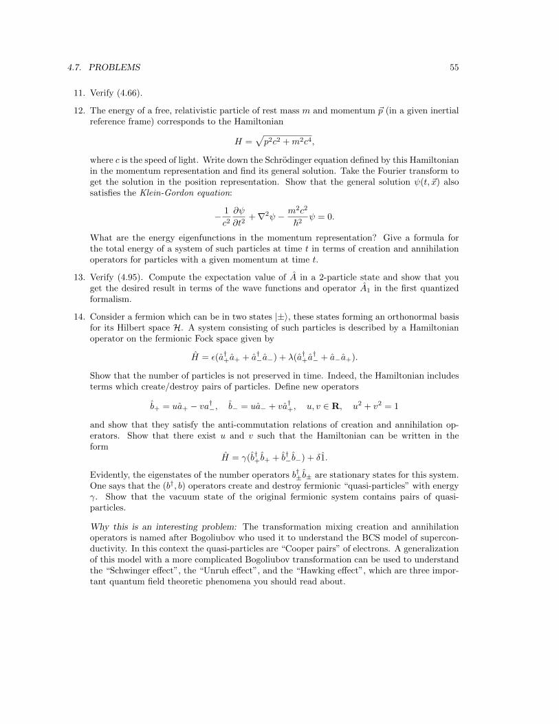
4.7. PROBLEMS 55
11. Verify (4.66).
12. The energy of a free, relativistic particle of rest mass m and momentum ~p (in a given inertialreference frame) corresponds to the Hamiltonian
H =√p2c2 +m2c4,
where c is the speed of light. Write down the Schrodinger equation defined by this Hamiltonianin the momentum representation and find its general solution. Take the Fourier transform toget the solution in the position representation. Show that the general solution ψ(t, ~x) alsosatisfies the Klein-Gordon equation:
− 1
c2∂ψ
∂t2+∇2ψ − m2c2
~2ψ = 0.
What are the energy eigenfunctions in the momentum representation? Give a formula forthe total energy of a system of such particles at time t in terms of creation and annihilationoperators for particles with a given momentum at time t.
13. Verify (4.95). Compute the expectation value of A in a 2-particle state and show that youget the desired result in terms of the wave functions and operator A1 in the first quantizedformalism.
14. Consider a fermion which can be in two states |±〉, these states forming an orthonormal basisfor its Hilbert space H. A system consisting of such particles is described by a Hamiltonianoperator on the fermionic Fock space given by
H = ε(a†+a+ + a†−a−) + λ(a†+a†− + a−a+).
Show that the number of particles is not preserved in time. Indeed, the Hamiltonian includesterms which create/destroy pairs of particles. Define new operators
b+ = ua+ − va†−, b− = ua− + va†+, u, v ∈ R, u2 + v2 = 1
and show that they satisfy the anti-commutation relations of creation and annihilation op-erators. Show that there exist u and v such that the Hamiltonian can be written in theform
H = γ(b†+b+ + b†−b−) + δ1.
Evidently, the eigenstates of the number operators b†±b± are stationary states for this system.One says that the (b†, b) operators create and destroy fermionic “quasi-particles” with energyγ. Show that the vacuum state of the original fermionic system contains pairs of quasi-particles.
Why this is an interesting problem: The transformation mixing creation and annihilationoperators is named after Bogoliubov who used it to understand the BCS model of supercon-ductivity. In this context the quasi-particles are “Cooper pairs” of electrons. A generalizationof this model with a more complicated Bogoliubov transformation can be used to understandthe “Schwinger effect”, the “Unruh effect”, and the “Hawking effect”, which are three impor-tant quantum field theoretic phenomena you should read about.

Chapter 5
Electromagnetic Fields
The photon is a quantum manifestation of the electromagnetic field. To see what that means wewill need to review some electrodynamics.
5.1 Maxwell equations
I will use the Gaussian system of electromagnetic units and I will let c denote the speed of lightin vacuum. The Maxwell equations are differential equations for the electric field ~E(~x, t), and the
magnetic field ~B(~x, t), which are defined by the force they exert on a test charge q at the point ~xat time t via the Lorentz force law:
~F (~x, t) = q
(~E(~x, t) +
1
c~v(t)× ~B(~x, t)
), (5.1)
where ~v(t) is the particle’s velocity at time t. Equation (5.1) is used to determine the motion of acharged particle in a given electromagnetic field assuming the effect of the particle on the field canbe neglected. Equation (5.1) can also be used to measure the electromagnetic field by observingthe motion of charged “test” particles.
The Lorentz force law tells us how the electromagnetic field affects electrically charged matter.The Maxwell equations tell us how the electrically charged matter affects the electromagnetic field.In macroscopic applications it is usually convenient to model the electric charges – the “sources”– of the electromagnetic field as a continuous electric charge density ρ(~x, t) and electric currentdensity ~j(~x, t). The Maxwell equations are
∇· ~E = 4πρ, (5.2)
∇· ~B = 0, (5.3)
∇× ~B − 1
c
∂ ~E
∂t=
4π
c~j, (5.4)
∇× ~E +1
c
∂ ~B
∂t= 0. (5.5)
I would like to spend a little time getting a feel for the basic features of these equations.
56

5.1. MAXWELL EQUATIONS 57
5.1.1 The basic structure of the Maxwell equations
First of all, the equations (5.2)–(5.5) are 8 coupled, first-order, partial differential equations (withconstant coefficients in Cartesian coordinates) for the 6 unknown functions contained in the com-
ponents of ~E and ~B.1 One usually views the Maxwell equations as equations which are used todetermine ~E and ~B for a given ρ and ~j. In this setting the equations for ~E and ~B are “linear-inhomogeneous” thanks to the “source terms” defined by ρ and ~j. Because the equations areinhomogeneous, it is not possible to superimpose solutions ( ~E1, ~B1) and ( ~E2, ~B2) to get new solu-tions without altering the charge and current densities. On the other hand, given any solution tothe Maxwell equations (for a given ρ and ~j) one can add any solution of the homogeneous Maxwellequations (where ρ = 0 = ~j) to get a new solution of the same inhomogeneous equations. If one issolving the Maxwell equations in a region of space where there are no sources, ρ = 0 and ~j = 0,then the equations are homogeneous and one can always superimpose solutions.
The equations (5.2) and (5.3) represent 2 “scalar” equations, while equations (5.4) and (5.5) are“vector equations”. A vector equation equates the components of two vectors. Thus the equations(5.4) and (5.5) each represent 3 (coupled) equations in which the x component of the left-hand sideis equated to the x component of the right hand side, and so on.
As already mentioned, the Maxwell equations are typically solved for ~E and ~B once the chargedensity and its motion (the current density) are specified. For example, one can let the chargedensity be that of a uniform ball of positive charge held fixed in space so that the current densityvanishes. As you might guess, the solution of these equations has vanishing magnetic field anda Coulomb-type electrostatic field outside the ball. (Do you remember what happens inside theball?) Note that this way of using the Maxwell equations assumes that the motion of the sources iscompletely known (or else, how could we specify ρ and ~j?). For many purposes this is a reasonablephysical assumption. But, strictly speaking, this is only an approximate description of electro-dynamics. As you can imagine, many applications (e.g., the electrodynamics of the ionosphere)will require us to also figure out how the sources are moving. This is a complicated problem andquite non-linear: the sources generate the electromagnetic field according to the Maxwell equations(5.2)–(5.5), the electromagnetic field affects the sources according to the Lorentz force law (5.1),but the motion of the charges determines the fields, and so on. Of course, if there are no sourcesthis is not an issue – at least classically. It turns out that in the quantum domain the sources cannever be completely ignored, although we won’t develop the theory far enough to see that.
Note that only 4 of the 8 Maxwell equations, (5.2) and (5.4), involve the sources. These are oftencalled the inhomogeneous equations because they are linear inhomogeneous in the unknowns. Theother 4 which do not involve the sources, (5.3) and (5.5), are likewise known as the homogeneousequations. The inhomogeneous equation (5.2) involving ρ – often called the Gauss law – shows thatthe charge density gives a divergence to the electric field. This is the way in which electric chargescreate electric fields. The Maxwell equation (5.3), on the other hand, shows that the magnetic fieldnever has a divergence. By analogy with the electric field, this equation can be viewed as statingthat there is no such thing as “magnetic charge”. The magnetic field can have a curl, however. Eq.(5.4) asserts that this corresponds to having a time varying electric field and/or having an electriccurrent density (moving charges). Thus a moving charge creates a magnetic field (the Biot-Savartlaw) and, as Maxwell first postulated, so does a time varying electric field. Finally, from (5.5), theelectric field can also have a curl, but only if there is a time varying magnetic field—a phenomenon
1Just by counting equations and unknowns one might worry that the system of equation is over-determined. Weshall see that this is not the case thanks to some fundamental identities satisfied by the equations.

58 CHAPTER 5. ELECTROMAGNETIC FIELDS
characterized by Faraday and one which is necessary for the existence of civilization as we know it.Note also that only 6 of the 8 equations, (5.4) and (5.5), involve a time derivative, that is, only
6 equations concern themselves with how the fields change in time. For this reason these equationsare called the evolution equations. The remaining two divergence equations are called constraintequations since they restrict the fields at any given time. It can be shown that the constraintequations only need to be satisfied once, i.e., at a single instant of time; the evolution equationswill guarantee they will be satisfied at later times. This is important because otherwise we wouldbe in danger of having too many equations (8) and not enough unknowns (6).
5.1.2 Continuity equation and conservation of electric charge
We now consider an important consistency condition that must be satisfied by the sources if theMaxwell equations are to admit any solution at all. This consistency condition says that a necessarycondition for the existence of a solution ( ~E, ~B) to the Maxwell equations is that the sources (ρ,~j)must satisfy a continuity equation.
Take the time derivative of (5.2) and interchange time and space derivatives to get
∇ · ∂~E
∂t= 4π
∂ρ
∂t.
Compare this result with the divergence of (5.4) :
−1
c∇ · ∂
~E
∂t=
4π
c∇ ·~j,
to find∂ρ
∂t+∇·~j = 0.
What this computation means is that the Maxwell equations have solutions for ~E and ~B only ifthe 4 functions ρ(~x, t) and ~j(~x, t) are chosen to satisfy the continuity equation (5.1.2) given above.Recall that this equation is a differential version of a conservation law; the conserved quantity inthis case being the electric charge. Explicitly, the total charge Q contained in a volume V at timet, defined by
Q =
∫V
dV ρ(~x, t),
changes in time according to the net flux of the current density ~j through the boundary S of V :
dQ
dt= −
∮S
~dS ·~j.
If the net flux of charge through the boundary (which may be “at infinity”) vanishes, then thecharge contained in V is constant in time. When we use the Maxwell equations to solve for theelectromagnetic field due to a given charge distribution, that distribution must be specified so thatcharge is conserved in the sense of (5.1.2) or else the equations cannot have a solution.2
2It is no accident that the Maxwell equations, in effect, force the conservation of electric charge. Indeed, ourcurrent field theoretic description of all fundamental interactions (electromagnetic, weak, strong, and gravitational)is geared to force such conservation laws through the use of variational principles and the “principle of local gaugeinvariance”. Unfortunately, a discussion of such ideas would be beyond the scope of this course.
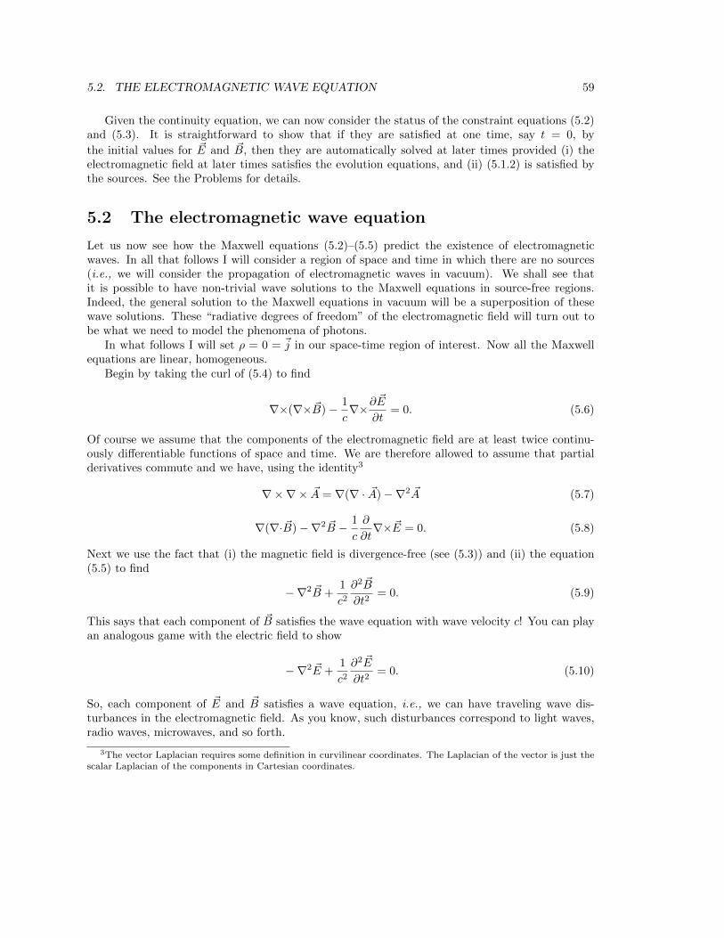
5.2. THE ELECTROMAGNETIC WAVE EQUATION 59
Given the continuity equation, we can now consider the status of the constraint equations (5.2)and (5.3). It is straightforward to show that if they are satisfied at one time, say t = 0, by
the initial values for ~E and ~B, then they are automatically solved at later times provided (i) theelectromagnetic field at later times satisfies the evolution equations, and (ii) (5.1.2) is satisfied bythe sources. See the Problems for details.
5.2 The electromagnetic wave equation
Let us now see how the Maxwell equations (5.2)–(5.5) predict the existence of electromagneticwaves. In all that follows I will consider a region of space and time in which there are no sources(i.e., we will consider the propagation of electromagnetic waves in vacuum). We shall see thatit is possible to have non-trivial wave solutions to the Maxwell equations in source-free regions.Indeed, the general solution to the Maxwell equations in vacuum will be a superposition of thesewave solutions. These “radiative degrees of freedom” of the electromagnetic field will turn out tobe what we need to model the phenomena of photons.
In what follows I will set ρ = 0 = ~j in our space-time region of interest. Now all the Maxwellequations are linear, homogeneous.
Begin by taking the curl of (5.4) to find
∇×(∇× ~B)− 1
c∇×∂
~E
∂t= 0. (5.6)
Of course we assume that the components of the electromagnetic field are at least twice continu-ously differentiable functions of space and time. We are therefore allowed to assume that partialderivatives commute and we have, using the identity3
∇×∇× ~A = ∇(∇ · ~A)−∇2 ~A (5.7)
∇(∇· ~B)−∇2 ~B − 1
c
∂
∂t∇× ~E = 0. (5.8)
Next we use the fact that (i) the magnetic field is divergence-free (see (5.3)) and (ii) the equation(5.5) to find
−∇2 ~B +1
c2∂2 ~B
∂t2= 0. (5.9)
This says that each component of ~B satisfies the wave equation with wave velocity c! You can playan analogous game with the electric field to show
−∇2 ~E +1
c2∂2 ~E
∂t2= 0. (5.10)
So, each component of ~E and ~B satisfies a wave equation, i.e., we can have traveling wave dis-turbances in the electromagnetic field. As you know, such disturbances correspond to light waves,radio waves, microwaves, and so forth.
3The vector Laplacian requires some definition in curvilinear coordinates. The Laplacian of the vector is just thescalar Laplacian of the components in Cartesian coordinates.
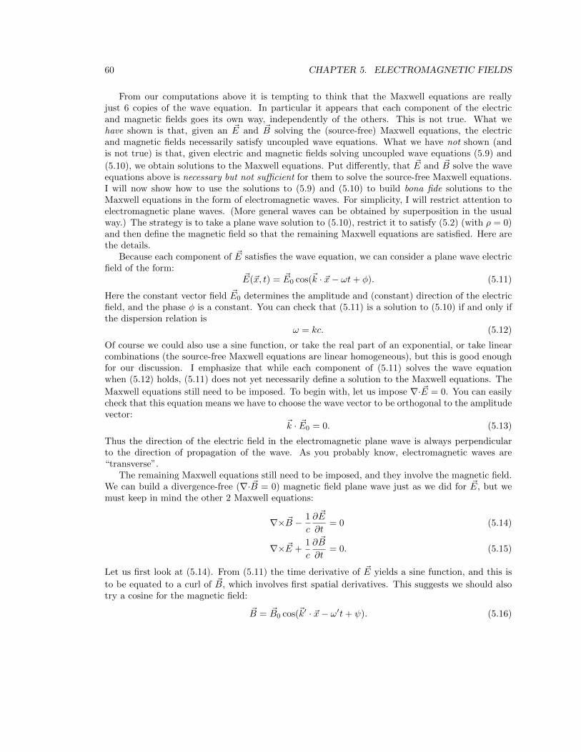
60 CHAPTER 5. ELECTROMAGNETIC FIELDS
From our computations above it is tempting to think that the Maxwell equations are reallyjust 6 copies of the wave equation. In particular it appears that each component of the electricand magnetic fields goes its own way, independently of the others. This is not true. What wehave shown is that, given an ~E and ~B solving the (source-free) Maxwell equations, the electricand magnetic fields necessarily satisfy uncoupled wave equations. What we have not shown (andis not true) is that, given electric and magnetic fields solving uncoupled wave equations (5.9) and
(5.10), we obtain solutions to the Maxwell equations. Put differently, that ~E and ~B solve the waveequations above is necessary but not sufficient for them to solve the source-free Maxwell equations.I will now show how to use the solutions to (5.9) and (5.10) to build bona fide solutions to theMaxwell equations in the form of electromagnetic waves. For simplicity, I will restrict attention toelectromagnetic plane waves. (More general waves can be obtained by superposition in the usualway.) The strategy is to take a plane wave solution to (5.10), restrict it to satisfy (5.2) (with ρ = 0)and then define the magnetic field so that the remaining Maxwell equations are satisfied. Here arethe details.
Because each component of ~E satisfies the wave equation, we can consider a plane wave electricfield of the form:
~E(~x, t) = ~E0 cos(~k · ~x− ωt+ φ). (5.11)
Here the constant vector field ~E0 determines the amplitude and (constant) direction of the electricfield, and the phase φ is a constant. You can check that (5.11) is a solution to (5.10) if and only ifthe dispersion relation is
ω = kc. (5.12)
Of course we could also use a sine function, or take the real part of an exponential, or take linearcombinations (the source-free Maxwell equations are linear homogeneous), but this is good enoughfor our discussion. I emphasize that while each component of (5.11) solves the wave equationwhen (5.12) holds, (5.11) does not yet necessarily define a solution to the Maxwell equations. The
Maxwell equations still need to be imposed. To begin with, let us impose ∇· ~E = 0. You can easilycheck that this equation means we have to choose the wave vector to be orthogonal to the amplitudevector:
~k · ~E0 = 0. (5.13)
Thus the direction of the electric field in the electromagnetic plane wave is always perpendicularto the direction of propagation of the wave. As you probably know, electromagnetic waves are“transverse”.
The remaining Maxwell equations still need to be imposed, and they involve the magnetic field.We can build a divergence-free (∇· ~B = 0) magnetic field plane wave just as we did for ~E, but wemust keep in mind the other 2 Maxwell equations:
∇× ~B − 1
c
∂ ~E
∂t= 0 (5.14)
∇× ~E +1
c
∂ ~B
∂t= 0. (5.15)
Let us first look at (5.14). From (5.11) the time derivative of ~E yields a sine function, and this is
to be equated to a curl of ~B, which involves first spatial derivatives. This suggests we should alsotry a cosine for the magnetic field:
~B = ~B0 cos(~k′ · ~x− ω′t+ ψ). (5.16)

5.2. THE ELECTROMAGNETIC WAVE EQUATION 61
To satisfy the wave equation we need the dispersion relation
ω′ = k′c. (5.17)
Because we want ∇· ~B = 0, we have to choose the wave vector and amplitude such that
~k′ · ~B0 = 0. (5.18)
It is easy to check that
∇× ~B = − ~B0 ×∇[cos(~k′ · ~x− ω′t+ ψ)
](5.19)
= ( ~B0 × ~k′) sin(~k′ · ~x− ω′t+ ψ). (5.20)
Next, we compute
1
c
∂ ~E
∂t=ω
c~E0 sin(~k · ~x− ωt+ φ). (5.21)
Thus (5.14) reduces to
ω
c~E0 sin(~k · ~x− ωt+ φ) = ~B0 × ~k′ sin(~k′ · ~x− ω′t+ ψ). (5.22)
Since this must hold at each location and time, it follows that
φ = ψ, (5.23)
~k′ = ~k, (5.24)
andω
c~E0 = −~k × ~B0. (5.25)
Let n be the unit vector in the direction of wave propagation:
n =~k
k, (5.26)
then we can write~E0 = −n× ~B0. (5.27)
Thus we see that the electric and magnetic fields must have the same wave vector, that is, they
have the same wavelengths (λ = 2π/k) and propagation directions~kk . Furthermore, from (5.27)
and the dispersion relation (5.12) it follows that:
• (1) The magnitudes of the electric and magnetic fields are equal4,
E0 = B0.
• (2) ~E and ~B are orthogonal, ~E · ~B = 0.
• (3) Each field is orthogonal to the propagation direction, ~E · n = 0 = ~B · n.
4Keep in mind we are using Gaussian units.
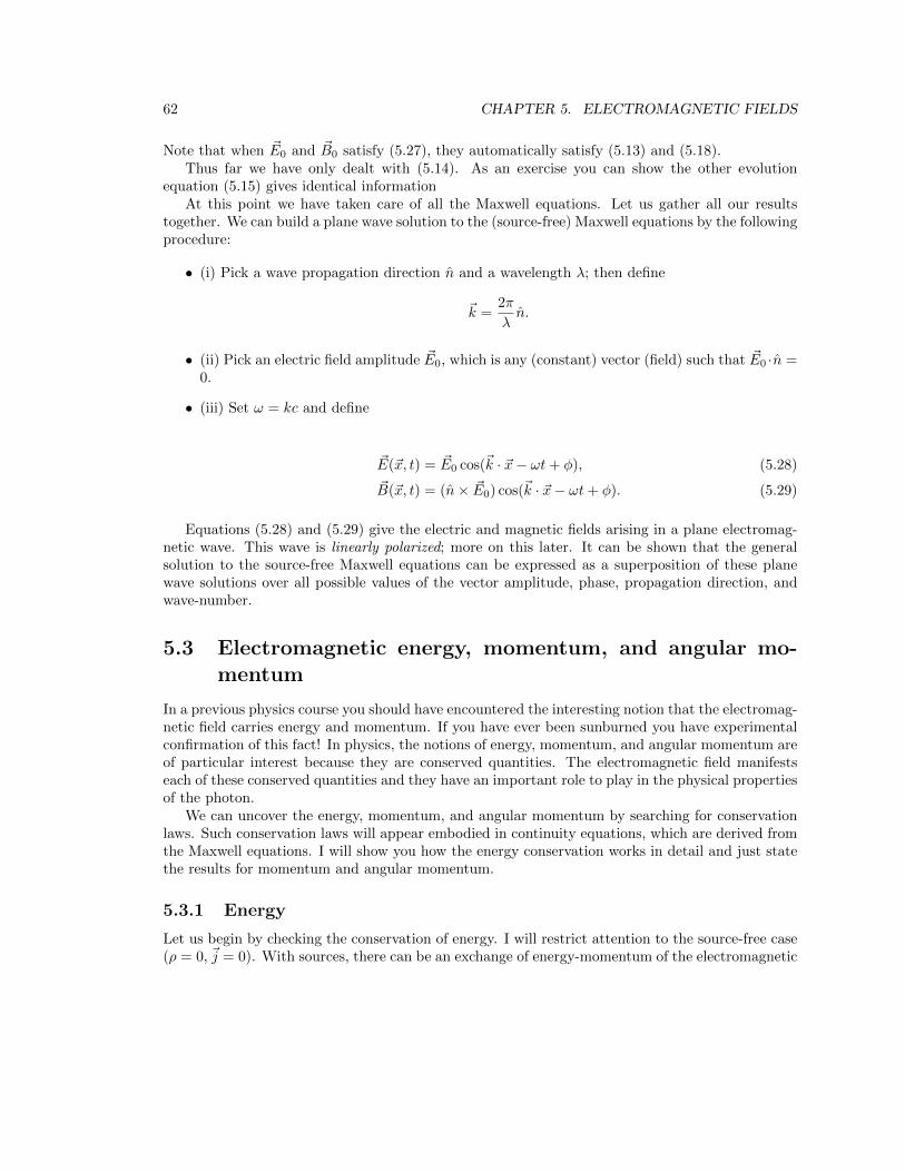
62 CHAPTER 5. ELECTROMAGNETIC FIELDS
Note that when ~E0 and ~B0 satisfy (5.27), they automatically satisfy (5.13) and (5.18).Thus far we have only dealt with (5.14). As an exercise you can show the other evolution
equation (5.15) gives identical informationAt this point we have taken care of all the Maxwell equations. Let us gather all our results
together. We can build a plane wave solution to the (source-free) Maxwell equations by the followingprocedure:
• (i) Pick a wave propagation direction n and a wavelength λ; then define
~k =2π
λn.
• (ii) Pick an electric field amplitude ~E0, which is any (constant) vector (field) such that ~E0 ·n =0.
• (iii) Set ω = kc and define
~E(~x, t) = ~E0 cos(~k · ~x− ωt+ φ), (5.28)
~B(~x, t) = (n× ~E0) cos(~k · ~x− ωt+ φ). (5.29)
Equations (5.28) and (5.29) give the electric and magnetic fields arising in a plane electromag-netic wave. This wave is linearly polarized; more on this later. It can be shown that the generalsolution to the source-free Maxwell equations can be expressed as a superposition of these planewave solutions over all possible values of the vector amplitude, phase, propagation direction, andwave-number.
5.3 Electromagnetic energy, momentum, and angular mo-mentum
In a previous physics course you should have encountered the interesting notion that the electromag-netic field carries energy and momentum. If you have ever been sunburned you have experimentalconfirmation of this fact! In physics, the notions of energy, momentum, and angular momentum areof particular interest because they are conserved quantities. The electromagnetic field manifestseach of these conserved quantities and they have an important role to play in the physical propertiesof the photon.
We can uncover the energy, momentum, and angular momentum by searching for conservationlaws. Such conservation laws will appear embodied in continuity equations, which are derived fromthe Maxwell equations. I will show you how the energy conservation works in detail and just statethe results for momentum and angular momentum.
5.3.1 Energy
Let us begin by checking the conservation of energy. I will restrict attention to the source-free case(ρ = 0, ~j = 0). With sources, there can be an exchange of energy-momentum of the electromagnetic

5.3. ELECTROMAGNETIC ENERGY, MOMENTUM, AND ANGULAR MOMENTUM 63
field with that of the sources and the story is a little longer than justified for our needs5. Since wehave used the symbols ρ and ~j to denote the electric charge density and electric current density,to avoid confusion I will use the symbols u and ~s to denote the energy density and energy currentdensity (also known as the “Poynting vector”) for the electromagnetic field. These are defined by(still in Gaussian units)
u =1
8π(E2 +B2), (5.30)
~s =c
4π~E × ~B. (5.31)
The claim is that (u,~s) satisfy∂u
∂t+∇·~s = 0 (5.32)
when ~E and ~B satisfy the (source-free) Maxwell equations.
To verify this, we need to use some vector identities. If ~A and ~C are any two vector fields thatdepend upon a variable t, we have that
∂
∂t(A2) =
∂
∂t( ~A · ~A) (5.33)
= 2 ~A · ∂~A
∂t, (5.34)
and∇·( ~A× ~C) = ~C · ∇× ~A− ~A · ∇×~C. (5.35)
Using these vector identities and the Maxwell equations, we have
4π∂u
∂t= ~E · ∂
~E
∂t+ ~B · ∂
~B
∂t(5.36)
= c ~E · ∇× ~B − c ~B · ∇× ~E, (5.37)
and4π∇·~s = c
(~B · ∇× ~E − ~E · ∇× ~B
), (5.38)
from which the result (5.32) follows immediately. Note we only needed the evolution equations toobtain (5.32).
We interpret u(~x, t) as the electromagnetic energy density at the point ~x and time t and thePoynting vector6 ~s as the energy current density. Define the total electromagnetic energy U in thevolume V to be the integral of the energy density u:
U :=
∫V
dV u =1
8π
∫V
dV(E2 +B2
). (5.39)
According to the continuity equation (5.32), the time rate of change of U is controlled by the fluxof the Poynting vector ~s through the boundary A of V :
dU
dt= −
∫A
~dA · ~s, (5.40)
5As you might expect on physical grounds, in order to get a conservation law in this case, one must keep track ofthe energy and momentum of the sources.
6 You should keep in mind that the Poynting vector is really a vector field.
64 CHAPTER 5. ELECTROMAGNETIC FIELDS
where~dA = N dA (5.41)
with N being the unit normal to the boundary surface of V .
It is worth computing the energy density and Poynting vector for the plane wave constructedabove in (5.28) and (5.29). You will find
u =1
4π(E0)2 cos2(~k · ~x− ωt+ φ), (5.42)
~s =c
4π(E0)2 cos2(~k · ~x− ωt+ φ) n. (5.43)
We see that the energy density of the wave is proportional to the amplitude-squared of the electricfield. We also see that that the Poynting vector lies along the direction of propagation n = ~k/k ofthe plane wave. Thus the flow of energy is along n. The continuity equation guarantees that if youintegrate u over a volume you will find that the total energy is changing according to the net fluxof ~s through the volume.
If, at the boundary of the region V , the fields are such that net the Poynting flux vanishes,then the energy contained in V will be constant in time. In particular, if the volume V in (5.39) istaken to be all space, we can view the boundary A as a sphere of infinite radius. If we consider anisolated system, so that the electric and magnetic fields vanish sufficiently rapidly at large distances(i.e., “at infinity”), then the flux of the Poynting vector will vanish as the radius of A is takento infinity. Thus the total electromagnetic energy of an isolated (and source-free) electromagneticfield is constant in time.
5.3.2 Momentum and angular momentum
Next let’s briefly look at electromagnetic momentum and angular momentum and their conservationlaws. It turns out that the momentum density ~π for the electromagnetic field is proportional to thePoynting vector:
~π =1
c2~s =
1
4πc~E × ~B. (5.44)
Using the Maxwell equations it can be shown that each Cartesian component πi of ~π satisfies
∂
∂tπi +
3∑j=1
∂
∂xj(τ ij) = 0, (5.45)
where τ ij are the components of a tensor which is minus the Maxwell stress tensor. It is not toohard to show this – you could try it, but I will leave a proof of this to a course in electrodynamics.It is perhaps intuitively clear that the Poynting vector, which defines the transport of energy shouldalso characterize the momentum. Each Cartesian component of ~π is a momentum density whichcan be integrated to get a conserved quantity. The volume integral of each Cartesian componentof ~π represents a conserved momentum ~P for the electromagnetic field:
~P =
∫V
dV1
4πc~E × ~B. (5.46)

5.4. ELECTROMAGNETIC POTENTIALS 65
The angular momentum density for the electromagnetic field is
~l = ~x× ~π =1
4πc~x× ( ~E × ~B). (5.47)
Notice that, as usual, the notion of angular momentum depends upon a reference point – here usedas a choice of origin – from which to define the position vector ~x. Each component of the angularmomentum density satisfies a continuity equation when the (source-free) Maxwell equations hold.The total angular momentum in a region V is
~L =1
4πc
∫V
dV[~x× ( ~E × ~B)
], (5.48)
where it must be understood that this formula is meant to be applied to the Cartesian componentsof the various vectors.
As you know, the Maxwell equations define a field theory in accord with the principles of specialrelativity. In this context, I should note that the energy, momentum, and angular momentum havebeen defined in a given inertial reference frame. Under a change of reference frame the energyand momentum mix; the reference frame independent quantity is the energy-momentum 4-vectorP = (U/c, ~P ). The behavior of the angular momentum under a change of inertial reference frameis somewhat more complicated; it is properly viewed as part of a relativistic angular momentumtensor. See, e.g., [5] for details.
5.4 Electromagnetic potentials
The homogeneous subset of the Maxwell equations
∇× ~E +1
c
∂ ~B
∂t= 0 (5.49)
and∇ · ~B = 0 (5.50)
are equivalent to the existence of a vector field, the vector potential ~A, and a scalar field, the scalarpotential φ, such that
~E = −1
c
∂ ~A
∂t−∇φ, ~B = ∇× ~A. (5.51)
With (φ, ~A) arbitrary, this is the general solution to the half of Maxwell’s equations given by (5.49),(5.50).7 Once we introduce the potentials the only remaining Maxwell equations to be solved arethe inhomogeneous ones (5.2), (5.4).
The potentials are far from uniquely determined by ~E and ~B. If (φ, ~A) are a set of potentials
which yield a given electromagnetic field ( ~E, ~B) via (5.51), then so are (exercise)
φ′ = φ− 1
c
∂Λ
∂t, (5.52)
7Technically, this is the general solution “in the small”; boundary conditions may put additional restrictions onthe potentials.

66 CHAPTER 5. ELECTROMAGNETIC FIELDS
~A′ = ~A+∇Λ, (5.53)
where Λ is any function of space and time. You can easily check this; just substitute (5.52), (5.53)into (5.49), (5.50) and watch the terms involving Λ drop out. This transformation between two setsof potentials for the same electromagnetic field is called a gauge transformation for historical reasonsthat I shall not go into. Under a gauge transformation the electromagnetic field is unchanged; wesay the electric and magnetic fields are gauge invariant. The notion of gauge invariance, whichjust seems like a technical detail in Maxwell theory, is actually pretty profound in physics. For ourpurposes, the freedom to redefine potentials via a gauge transformation means that we have somefreedom to put the potentials into a convenient form by making a “choice of gauge”.
For our purposes we will use potentials which are in the radiation gauge. What this means isas follows. Any electromagnetic field ( ~E, ~B) in the absence of sources can be described by a set ofpotentials such that
φ = 0, ∇ · ~A = 0. (5.54)
To see this, given any potentials φ1 and ~A1 for the given ( ~E, ~B), we can make a gauge transformationusing a function Λ1 which at each time t is a solution to the Poisson equation
∇2Λ1 = −∇ · ~A1. (5.55)
The result is a set of potentials (φ2, ~A2) where
∇ · ~A2 = 0. (5.56)
Such potentials are said to be in the Coulomb gauge. (The Coulomb gauge is available whether ornot the sources vanish.) One can make a further gauge transformation by a function Λ2, preservingthe Coulomb gauge, provided
∇2Λ2 = 0. (5.57)
To gauge transform the scalar potential to zero one should choose
Λ2 = c
∫dt φ2. (5.58)
But this choice will satisfy (5.57) only if ∇2φ2 = 0. If there are sources this need not be the casebecause in the Coulomb gauge
∇ · ~E = 4πρ ⇐⇒ ∇2φ = −4πρ. (5.59)
But in a region where ρ = 0 there is no obstruction to transforming the scalar potential to zero.In the radiation gauge the electromagnetic fields are determined by the electromagnetic poten-
tials according to8
~E = −1
c
∂ ~A
∂t, ~B = ∇× ~A. (5.60)
8 This might amuse you (at least a little). In electrostatics we have ~B = 0 and∇× ~E = 0; it is conventional to work
in a gauge in which ~A = 0 so that the static electric field is given by ~E = −∇φ. This is certainly the most convenientway to analyze electrostatics, but one could opt to set the scalar potential to zero and use a time-dependent (andcurl-free) vector potential if so-desired.

5.5. ROLE OF THE SOURCES 67
Any gauge transformation Λ which preserves the radiation gauge must satisfy
∂Λ
∂t= 0, ∇2Λ = 0. (5.61)
With suitable boundary conditions one can ensure that Λ = const. is the only solution. Such gaugetransformations are trivial – they do not transform anything and we identify them with the identitytransformation. In this way the potentials can be uniquely associated to the electromagnetic fieldin the radiation gauge.
By using potentials half the Maxwell equations are satisfied. The remaining equations are (5.2)and (5.4) with ρ = 0 = ~j,
∇ · ~E = 0, (5.62)
and
∇× ~B − 1
c
∂ ~E
∂t= 0 (5.63)
Substituting for ( ~E, ~B) using (5.60 shows that (5.62) is satisfied in the radiation gauge and (5.63)becomes
1
c2∂2 ~A
∂t2−∇2 ~A = 0, ∇ · ~A = 0 (5.64)
where I used the vector identity (5.7). Thus the source-free Maxwell equations can be expressed asa wave equation for a “transverse” vector field via the radiation gauge.
5.5 Role of the sources
Let me briefly comment on how the sources enter into this game. Allowing for the presence of sourcesmeans we cannot set φ = 0, but we can still use the Coulomb gauge ∇· ~A = 0. In the Coulomb gaugethe scalar potential satisfies the Poisson equation (5.59). With appropriate boundary conditionsthis will uniquely determine the scalar potential in terms of the charge density. Having eliminatedthe scalar potential in this way, the electromagnetic degrees of freedom will (still) reside in thetransverse vector potential, which now satisfies
1
c2∂2 ~A
∂t2−∇2 ~A =
4π
c~j, ∇ · ~A = 0. (5.65)
As you may know from a class in electrodynamics, the solution of these equations can be obtainedas
~A = ~A~j + ~A0, (5.66)
where ~A~j is determined by ~j using the retarded Green function and ~A0 is any solution to thesource-free equations. In this sense we say that the solutions to the source-free equations representthe “degrees of freedom” of the electromagnetic field. It is these degrees of freedom which becomeinterpreted in terms of photons in the quantum theory.
As a simple example of all this, suppose the source consists of a point charge q at rest at theorigin (in a given inertial reference frame) so that
ρ(~x, t) = qδ(~x), ~j(~x, t) = 0. (5.67)

68 CHAPTER 5. ELECTROMAGNETIC FIELDS
Let the spatial region of interest be all of Euclidean space, with fields vanishing “at infinity”. Thescalar potential is then the usual Coulomb field, φ = q/|~x|, and we have ~A~j = 0. The homogeneous
solutions ~A0 are unrestricted (except by the asymptotic conditions). The presence of ~A0 representsthe presence of electromagnetic radiation in addition to the Coulomb field. All together, this isthe classical model of the electromagnetic field experienced by an electron in a hydrogenic atomin the presence of radiation. In Chapter 7 we shall use the quantum version of ~A0 to understandspontaneous emission.
5.6 Solution to the source-free Maxwell equations
The general solution to (5.64) can be obtained from some Fourier analysis. Make a Fourier decom-
position of ~A at each time t:
~A(~x, t) =1
(2π)3/2
∫R3
d3k ~A(~k, t)ei~k·~x, (5.68)
~A(~k, t) =1
(2π)3/2
∫all space
d3x ~A(~x, t)e−i~k·~x. (5.69)
For notational simplicity I am denoting integrals over Fourier space by∫R3
d3k ≡∫ ∞−∞
dkx
∫ ∞−∞
dky
∫ ∞−∞
dkz. (5.70)
At each time t the Fourier transform ~A(~k, t) is a vector of complex functions of the real variables~k = (kx, ky, kz). Because ~A(~x, t) is real its transform must satisfy
~A(~k, t)∗ = ~A(−~k, t). (5.71)
The gauge condition which ~A satisfies implies that its Fourier transform is orthogonal to ~k:
∇ · ~A = 0 ⇐⇒ ~k · ~A(~k, t) = 0. (5.72)
In terms of the Fourier transform the electric and magnetic fields take the form:
~E = −1
c
∂ ~A
∂t= − 1
(2π)3/2
∫R3
d3k1
c
∂
∂t~A(~k, t)ei
~k·~x, (5.73)
~B = ∇× ~A =i
(2π)3/2
∫R3
d3k [~k × ~A(~k, t)]ei~k·~x. (5.74)
Substitution of the Fourier expansion (5.68) into (5.64) shows that these equations are equivalentto
~A(~k, t) = −ω2(k) ~A(~k, t), ~k · ~A(~k, t) = 0, (5.75)
whereω(k) = kc. (5.76)
Thus the real and imaginary parts of each of the two independent vector components of each Fouriercoefficient of ~A behaves like a harmonic oscillator with frequency ω(k).

5.7. ENERGY AND MOMENTUM, REVISITED 69
Heuristically, you can think of the Fourier transform (5.69) as a generalization to a continuousinfinity of degrees of freedom of the linear change of variables (2.21) to the displacements of the
normal modes of vibration. In this generalization, for a given ~k (the real and imaginary part of)
each component of ~A~k(t) orthogonal to ~k defines a normal mode of vibration. I will spare you somesuspense and reveal that, in what follows, we will construct the quantum theory of these oscillators~A~k and identify the states of the system with photon states. In this way a photon is built fromquantum normal modes of vibration of the electromagnetic field.
With the harmonic oscillator interpretation in mind, we can write the solution of (5.75) in termsof complex amplitudes of vibration as follows:
~A(~k, t) =
2∑σ=1
√2π~ck
[aσ(~k) ~εσ(~k) e−iω(k)t + a∗σ(−~k) ~εσ(−~k) eiω(k)t]. (5.77)
Here, for each ~k, the vectors ~εσ(~k), σ = 1, 2 are two mutually orthogonal real-valued unit vectors,
each orthogonal to ~k,
~εσ(~k) · ~ετ (~k) = δστ , ~εσ(~k) · ~k = 0, ~ε1(~k)× ~ε2(~k) =~k
k(5.78)
The variables aσ(~k) carry the information about the amplitude contribution for each wave with
wave vector ~k as well as the polarization contribution. Note that we have used ~ to define thenew variables. From a purely classical electromagnetic point of view this is a bit strange, but it isconvenient for the quantum treatment we will give. For now, just think of the use of ~ as a way ofgiving convenient units to the amplitudes aσ(~k), which are dimensionless (exercise).
We have now completely solved the source-free Maxwell equations in terms of a vector potentialin the radiation gauge. To get the electric and magnetic fields one should substitute ~A as definedin (5.77)– (5.78) into (5.68) to get the vector potential ~A(~x, t) in the radiation gauge:
~A(~x, t) =1
(2π)3/2
∫R3
d3k
2∑σ=1
√2π~ck
[aσ(~k) ~εσ(~k) ei~k·~x−iω(k)t + a∗σ(~k) ~εσ(~k) e−i
~k·~x+iω(k)t]. (5.79)
Substitute this potential into (5.60) to get ~E and ~B solving the source-free Maxwell equations.All solutions to the source-free Maxwell equations are obtained by making suitable choices for thecomplex amplitude aσ(~k).
5.7 Energy and momentum, revisited
In this section I will express the energy and momentum of the electromagnetic field in terms of thecomplex amplitudes for the harmonically oscillating normal modes derived in the previous section.
The energy for the electromagnetic field is given by
U =1
8π
∫all space
d3x (E2 +B2), (5.80)
where it is understood the electric and magnetic fields are expressed in terms of the potentials via(5.51).9 It is well worth knowing that in the Hamiltonian formalism for the electromagnetic field
9Of course we will have restrict attention to fields which vanish at spatial infinity so that the integral exists.
70 CHAPTER 5. ELECTROMAGNETIC FIELDS
(see, e.g., [5]) the quantity − ~E is ultimately identified with the momentum canonically conjugate
to ~A. You can then see from this energy formula that the E2 term is analogous to kinetic energy inNewtonian mechanics, while the B2 term is akin to potential energy. This perspective is underscoredby the expression of the energy in terms of potentials. The “kinetic” and “potential” energies are
1
8π
∫all space
d3xE2 =1
8π
∫all space
d3x1
c2
(∂ ~A
∂t
)2
(5.81)
1
8π
∫all space
d3xB2 =1
8π
∫all space
d3x(∇× ~A
)2. (5.82)
Substituting in the Fourier expansion (5.68) and using (5.73), (5.74) yields
U =1
8πc2
∫R3
d3k| ~A~k|
2 + k2c2|A~k|2. (5.83)
This form for U is of course consistent with our identification of the real and imaginary parts of thecomponents of ~A~k for each ~k as representing harmonic oscillators with frequency kc. In particular,the integral over Fourier space generalizes the sum over normal modes which would appear in theenergy for a system of coupled oscillators.
It will be useful later to have the energy expressed in terms of the complex amplitudes. Using(5.77) and its consequence
1
c~A~k = −i
√2π~kc
∑σ
[aσ(~k)εσ(~k)e−iωt − a∗σ(−~k)εσ(−~k)eiωt
], (5.84)
we get, after just a little algebra,
U =
∫R3
d3k∑σ
~ω(k) a∗σ(~k)aσ(~k). (5.85)
You can use similar computations to get a nice formula for the momentum of the electromag-netic field. Recall that the momentum density for the electromagnetic field is given by (5.44).Substituting the Fourier form of the vector potential in terms of complex amplitudes as before, youwill find
~P ≡∫all space
d3x1
c~E × ~B =
∫d3k
∑σ
~~k a∗σ(~k)aσ(~k). (5.86)
Hopefully, these very simple formulas for the energy and momentum justify all the effort thatwent into deriving them. Evidently, the electromagnetic field is a continuous family of coupledoscillators. The a and a∗ variables are the complex amplitudes for the normal modes of vibrationfor the electromagnetic field. The fact that there are infinitely many of these oscillators is novel,and is needed to build up (by superposition) all the familiar (and not manifestly oscillator-like)electromagnetic phenomena. The formulas for the energy and momentum show that the normalmode of vibration with wave vector ~k and polarization σ is characterized by an intensity |a~k,σ|
2
and carries energy ~ω and momentum ~~k. The appearance of ~ at this point does not indicate atruly quantum mechanical result, but rather our peculiar normalization — at this juncture — ofthe complex amplitudes.
5.8. ANGULAR MOMENTUM, REVISITED 71
5.8 Angular momentum, revisited
The angular momentum of the electromagnetic field,
~L =1
4πc
∫all space
d3x[~x× ( ~E × ~B)
](5.87)
is a little more complicated than the energy and momentum since it can be viewed as being composedof a reference frame dependent “orbital” part and an intrinsic “spin” part. The spin part has arelativistically invariant meaning and will correspond to the helicity of photons, so we want to havea look at it here.
To decompose the angular momentum into its orbital and spin parts we will need a slightlycomplicated vector identity:
[~x× ( ~E × ~B)]i = ( ~E × ~A)i + ~E · (~x×∇)i ~A+∇ · [( ~A× ~x)i ~E], (5.88)
where the index i labels the Cartesian components of the indicated vectors. The only good way Iknow to derive this identity is to use ~B = ∇× ~A and then use the fact that Cartesian componentsof the cross product and curl can be expressed in terms of the alternating symbol:
(~C × ~D)i = εijkCjDk, (∇× ~D)i = εi
jk∂
∂xjDk, (5.89)
where repeated indices are summed over. Then one has to use the identity
εijkεilm = δjl δkm − δkl δjm. (5.90)
With this identity in hand, one can decompose the angular momentum integrand into the threeterms shown in (5.88). The last term in (5.88) is a divergence and by the divergence theorem
can be transformed to the boundary of the region – spatial infinity. Assuming that ~A vanishesrapidly enough at infinity this term will not contribute. The second term in (5.88) depends upon areference point and can be viewed as giving the density of “orbital” angular momentum. The firstterm in (5.88) does not depend upon a reference point and yields the “intrinsic” or “spin” angularmomentum density.
Let us express the intrinsic part of the angular momentum,
~J =1
4πc
∫all space
d3x ( ~E × ~A), (5.91)
in terms of the Fourier amplitudes. Substituting ~E = − 1c∂A∂t and then using the formula (5.77) we
get
~J = i~∫R3
d3k~k
k
[a∗1(~k)a2(~k)− a∗2(~k)a1(~k)
]. (5.92)
To put this result in a more useful form, introduce the following complex basis for the vector spaceorthogonal to ~k:
~ε+(~k) = − 1√2
(~ε1(~k) + i~ε2(~k) (5.93)
~ε−(~k) =1√2
(~ε1(~k)− i~ε2(~k) (5.94)
72 CHAPTER 5. ELECTROMAGNETIC FIELDS
and define corresponding amplitudes
a+(~k) = − 1√2
(a1(~k)− ia2(~k)) (5.95)
a−(~k) =1√2
(a1(~k) + ia2(~k)) (5.96)
so thata1(~k)~ε1(~k) + a2(~k)~ε2(~k) = a+(~k)~ε+(~k) + a−(~k)~ε−(~k), (5.97)
andi(a∗1(~k)a2(~k)− a∗2(~k)a1(~k)) = a∗+(~k)a+(~k)− a∗−(~k)a−(~k). (5.98)
The functions a±(~k) are the complex amplitudes for plane waves with circular polarization. Wethen have
~J = ~∫R3
d3k~k
k(a∗+(~k)a+(~k)− a∗−(~k)a−(~k)). (5.99)
The clockwise and counter-clockwise amplitudes for each ~k contribute equally in magnitude butoppositely in sign to the “spin” part of the angular momentum. For each ~k the intrinsic angularmomentum density vector is directed along the wave vector ~k; its magnitude – proportional to(5.98) – can be shown to be invariant under a change of inertial reference frame. This relativistic
invariant (divided by ~) is known as the helicity of the plane wave with wave vector ~k. I will denote
the helicity of a wave with wave vector ~k by
J (~k) = a∗+(~k)a+(~k)− a∗−(~k)a−(~k). (5.100)
5.9 Periodic boundary conditions
As shown above, the states of the electromagnetic field (in the absence of sources) can be identifiedwith a collection of harmonic oscillators, which are playing the role of normal modes of vibrationfor the system. This interpretation is somewhat figurative since the normal modes are (1) infinite
in number and (2) labeled by a continuous set of variables ~k. There is nothing to be done about(1); in contrast to a mechanical system, a field has an infinite number of degrees of freedom. Butthere is something we can do about (2) which will be convenient in the next chapter.
Imagine putting the electromagnetic field in a large but finite cube of edge length L
0 ≤ x ≤ L, 0 ≤ y ≤ L, 0 ≤ z ≤ L, (5.101)
and imposing periodic boundary conditions. The idea is that for large enough L any physicallyrelevant results will differ insignificantly from the results obtained in the limit L → ∞.10 We canuse this artifice to render the normal modes into a discrete (if infinite) set. To be sure, it is notnecessary to do this. I just thought it might make the upcoming construction of photons a littleeasier to assimilate if we kept the description a little closer to that of a mechanical system by usingthe artifice of periodic boundary conditions. So let me just summarize here what happens to thenormal modes in this case.
10Other boundary conditions, e.g., Dirichlet conditions, would serve as well. Periodic boundary conditions areadvantageous since they allow for mode functions which are simple exponentials.
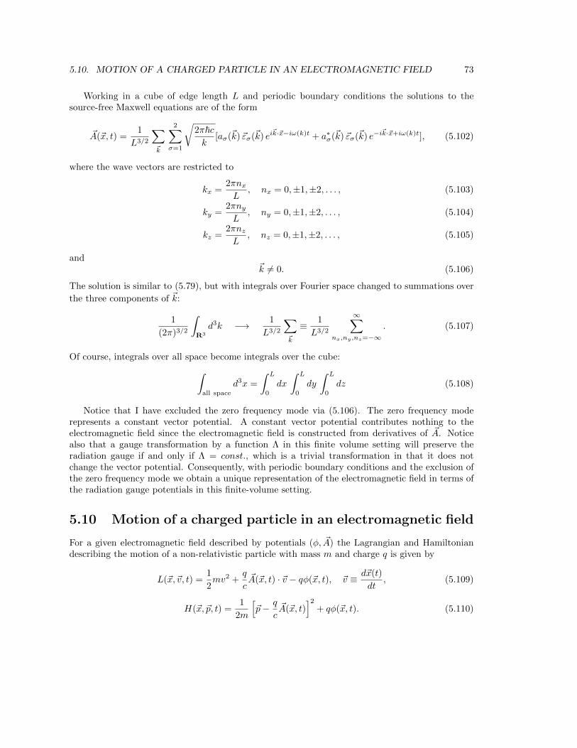
5.10. MOTION OF A CHARGED PARTICLE IN AN ELECTROMAGNETIC FIELD 73
Working in a cube of edge length L and periodic boundary conditions the solutions to thesource-free Maxwell equations are of the form
~A(~x, t) =1
L3/2
∑~k
2∑σ=1
√2π~ck
[aσ(~k) ~εσ(~k) ei~k·~x−iω(k)t + a∗σ(~k) ~εσ(~k) e−i
~k·~x+iω(k)t], (5.102)
where the wave vectors are restricted to
kx =2πnxL
, nx = 0,±1,±2, . . . , (5.103)
ky =2πnyL
, ny = 0,±1,±2, . . . , (5.104)
kz =2πnzL
, nz = 0,±1,±2, . . . , (5.105)
and~k 6= 0. (5.106)
The solution is similar to (5.79), but with integrals over Fourier space changed to summations over
the three components of ~k:
1
(2π)3/2
∫R3
d3k −→ 1
L3/2
∑~k
≡ 1
L3/2
∞∑nx,ny,nz=−∞
. (5.107)
Of course, integrals over all space become integrals over the cube:∫all space
d3x =
∫ L
0
dx
∫ L
0
dy
∫ L
0
dz (5.108)
Notice that I have excluded the zero frequency mode via (5.106). The zero frequency moderepresents a constant vector potential. A constant vector potential contributes nothing to theelectromagnetic field since the electromagnetic field is constructed from derivatives of ~A. Noticealso that a gauge transformation by a function Λ in this finite volume setting will preserve theradiation gauge if and only if Λ = const., which is a trivial transformation in that it does notchange the vector potential. Consequently, with periodic boundary conditions and the exclusion ofthe zero frequency mode we obtain a unique representation of the electromagnetic field in terms ofthe radiation gauge potentials in this finite-volume setting.
5.10 Motion of a charged particle in an electromagnetic field
For a given electromagnetic field described by potentials (φ, ~A) the Lagrangian and Hamiltoniandescribing the motion of a non-relativistic particle with mass m and charge q is given by
L(~x,~v, t) =1
2mv2 +
q
c~A(~x, t) · ~v − qφ(~x, t), ~v ≡ d~x(t)
dt, (5.109)
H(~x, ~p, t) =1
2m
[~p− q
c~A(~x, t)
]2+ qφ(~x, t). (5.110)

74 CHAPTER 5. ELECTROMAGNETIC FIELDS
The Euler-Lagrange equations yield the Lorentz force law:
md~v
dt= q ~E(~x, t) +
q
c~v × ~B(~x, t). (5.111)
The Hamilton equations,d~x
dt=∂H
∂~p=
1
m(~p− q
c~A), (5.112)
d~p
dt= −∂H
∂~x. (5.113)
are equivalent to (5.111).The functional forms of both the Lagrangian and the Hamiltonian change when a gauge trans-
formation is made. Despite this, the equations of motion evidently manage to be invariant undergauge transformations. This can be understood in the Lagrangian formalism by the fact that undera gauge transformation the Lagrangian changes only by addition of a total time derivative, whichdoes not alter the Euler-Lagrange equations. From the Hamiltonian perspective, the change in theHamiltonian corresponds to that induced by a canonical transformation, and canonical transforma-tions yield equivalent equations of motion.
5.11 Problems
1. Show that the magnetic field satisfies the same wave equation as the electric field.
2. The constraint equations are the two scalar Maxwell equations (5.2), (5.3), which do notinvolve time derivatives. The evolution equations are the remaining Maxwell equations (5.4),(5.5), involving the time derivatives. Show that if the constraint equations are satisfied atany one time, and the electromagnetic field at any later time is obtained by solving theevolution equations with the sources satisfying the continuity equation, then the constraintequations are satisfied at any later time. Thus the constraints can be viewed as restrictionson the initial data for the evolution equations. (Hint: Show that the time derivative of theconstraints vanishes.)
3. Verify that the momentum and angular momentum are conserved when the source-free Maxwellequations are satisfied.
4. A quantum particle with mass m and charge q is moving in a given electromagnetic fieldrepresented by potentials (φ(~x, t), ~A(~x, t)). The motion of the particle is described by theHamiltonian operator:
H =1
2m
[~p− q
c~A(~x, t)
]2+ qφ(~x, t). (5.114)
Solve the eigenvalue problem for this Hamiltonian in the case of a static, uniform magneticfield ~B = Bz, B = const., which can be described by the potentials
φ = 0, ~A =1
2~B × ~x. (5.115)
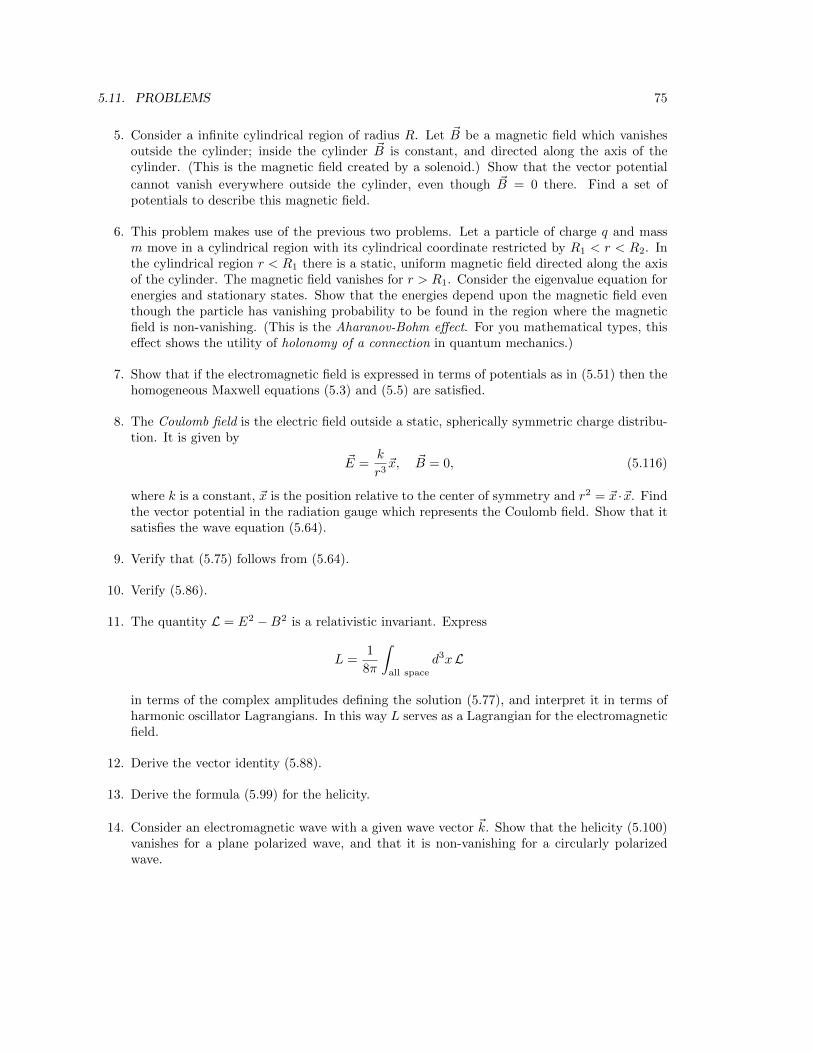
5.11. PROBLEMS 75
5. Consider a infinite cylindrical region of radius R. Let ~B be a magnetic field which vanishesoutside the cylinder; inside the cylinder ~B is constant, and directed along the axis of thecylinder. (This is the magnetic field created by a solenoid.) Show that the vector potential
cannot vanish everywhere outside the cylinder, even though ~B = 0 there. Find a set ofpotentials to describe this magnetic field.
6. This problem makes use of the previous two problems. Let a particle of charge q and massm move in a cylindrical region with its cylindrical coordinate restricted by R1 < r < R2. Inthe cylindrical region r < R1 there is a static, uniform magnetic field directed along the axisof the cylinder. The magnetic field vanishes for r > R1. Consider the eigenvalue equation forenergies and stationary states. Show that the energies depend upon the magnetic field eventhough the particle has vanishing probability to be found in the region where the magneticfield is non-vanishing. (This is the Aharanov-Bohm effect. For you mathematical types, thiseffect shows the utility of holonomy of a connection in quantum mechanics.)
7. Show that if the electromagnetic field is expressed in terms of potentials as in (5.51) then thehomogeneous Maxwell equations (5.3) and (5.5) are satisfied.
8. The Coulomb field is the electric field outside a static, spherically symmetric charge distribu-tion. It is given by
~E =k
r3~x, ~B = 0, (5.116)
where k is a constant, ~x is the position relative to the center of symmetry and r2 = ~x ·~x. Findthe vector potential in the radiation gauge which represents the Coulomb field. Show that itsatisfies the wave equation (5.64).
9. Verify that (5.75) follows from (5.64).
10. Verify (5.86).
11. The quantity L = E2 −B2 is a relativistic invariant. Express
L =1
8π
∫all space
d3xL
in terms of the complex amplitudes defining the solution (5.77), and interpret it in terms ofharmonic oscillator Lagrangians. In this way L serves as a Lagrangian for the electromagneticfield.
12. Derive the vector identity (5.88).
13. Derive the formula (5.99) for the helicity.
14. Consider an electromagnetic wave with a given wave vector ~k. Show that the helicity (5.100)vanishes for a plane polarized wave, and that it is non-vanishing for a circularly polarizedwave.

76 CHAPTER 5. ELECTROMAGNETIC FIELDS
15. Consider an interval [0, L] and the set of smooth, periodic functions on it. Show that when“integrated” against such functions, the following expression defines a delta function:
δ(x, y) =1
L
∞∑n=0
ein(x−y)2πL . (5.117)
16. In the context of periodic boundary conditions, show that the radiation gauge vector potentialis uniquely determined by the electromagnetic field. (Hint: Show that a gauge transformation~A→ ~A+∇Λ which preserves the divergence condition ∇ · ~A = 0 is necessarily trivial.)
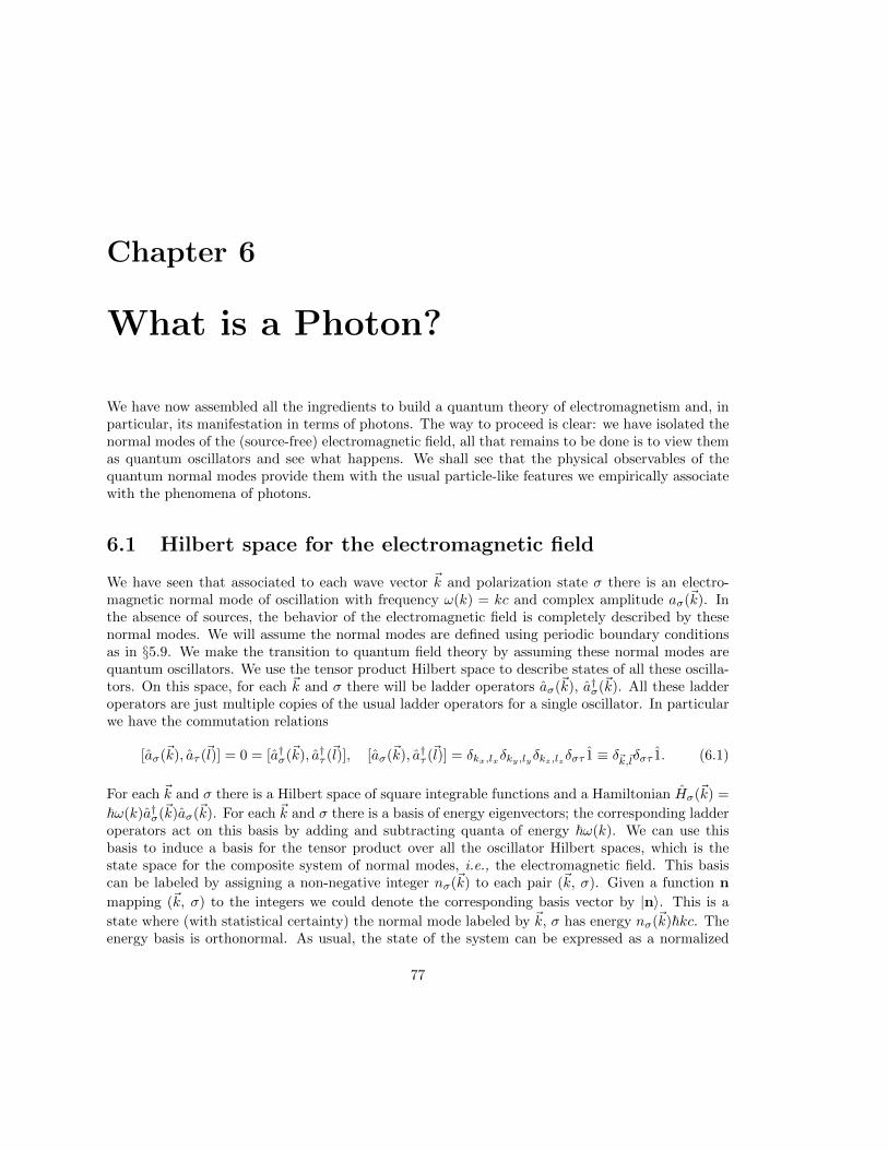
Chapter 6
What is a Photon?
We have now assembled all the ingredients to build a quantum theory of electromagnetism and, inparticular, its manifestation in terms of photons. The way to proceed is clear: we have isolated thenormal modes of the (source-free) electromagnetic field, all that remains to be done is to view themas quantum oscillators and see what happens. We shall see that the physical observables of thequantum normal modes provide them with the usual particle-like features we empirically associatewith the phenomena of photons.
6.1 Hilbert space for the electromagnetic field
We have seen that associated to each wave vector ~k and polarization state σ there is an electro-magnetic normal mode of oscillation with frequency ω(k) = kc and complex amplitude aσ(~k). Inthe absence of sources, the behavior of the electromagnetic field is completely described by thesenormal modes. We will assume the normal modes are defined using periodic boundary conditionsas in §5.9. We make the transition to quantum field theory by assuming these normal modes arequantum oscillators. We use the tensor product Hilbert space to describe states of all these oscilla-tors. On this space, for each ~k and σ there will be ladder operators aσ(~k), a†σ(~k). All these ladderoperators are just multiple copies of the usual ladder operators for a single oscillator. In particularwe have the commutation relations
[aσ(~k), aτ (~l)] = 0 = [a†σ(~k), a†τ (~l)], [aσ(~k), a†τ (~l)] = δkx,lxδky,lyδkz,lzδστ 1 ≡ δ~k,~lδστ 1. (6.1)
For each ~k and σ there is a Hilbert space of square integrable functions and a Hamiltonian Hσ(~k) =
~ω(k)a†σ(~k)aσ(~k). For each ~k and σ there is a basis of energy eigenvectors; the corresponding ladderoperators act on this basis by adding and subtracting quanta of energy ~ω(k). We can use thisbasis to induce a basis for the tensor product over all the oscillator Hilbert spaces, which is thestate space for the composite system of normal modes, i.e., the electromagnetic field. This basiscan be labeled by assigning a non-negative integer nσ(~k) to each pair (~k, σ). Given a function n
mapping (~k, σ) to the integers we could denote the corresponding basis vector by |n〉. This is a
state where (with statistical certainty) the normal mode labeled by ~k, σ has energy nσ(~k)~kc. Theenergy basis is orthonormal. As usual, the state of the system can be expressed as a normalized
77
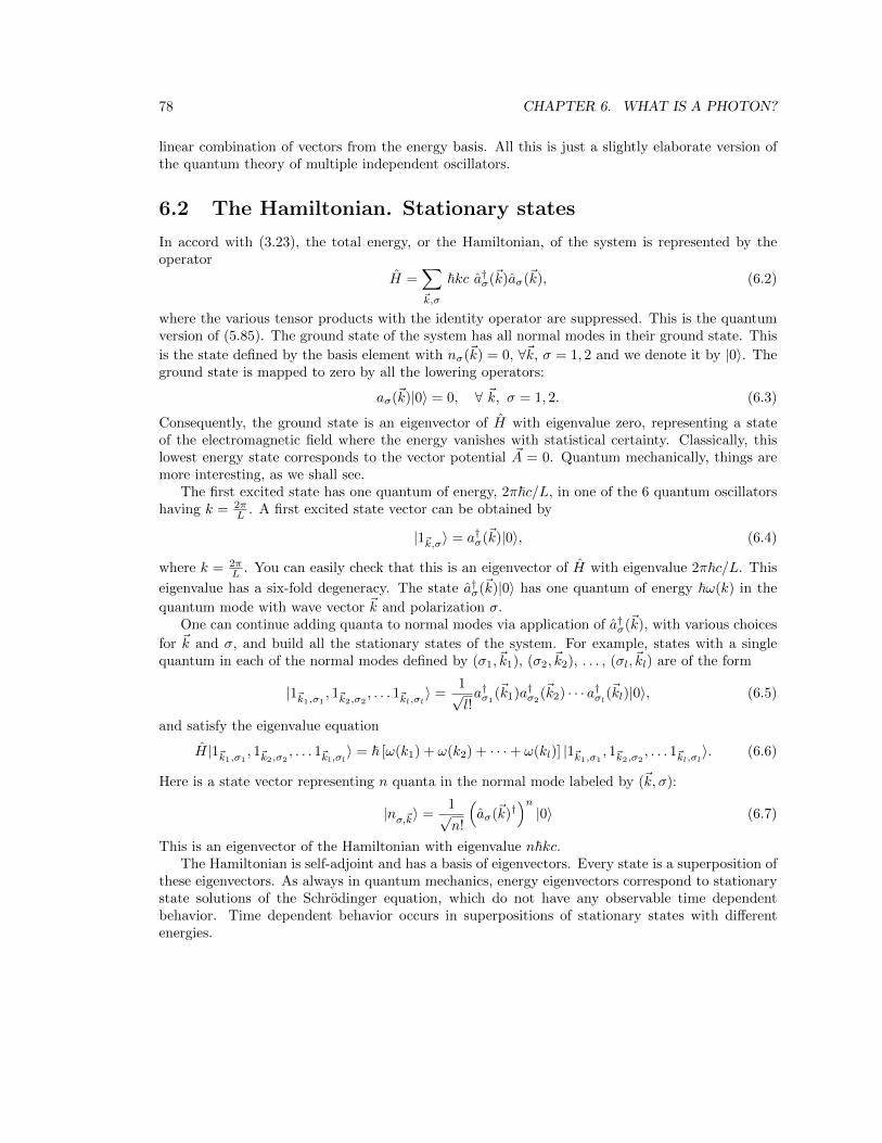
78 CHAPTER 6. WHAT IS A PHOTON?
linear combination of vectors from the energy basis. All this is just a slightly elaborate version ofthe quantum theory of multiple independent oscillators.
6.2 The Hamiltonian. Stationary states
In accord with (3.23), the total energy, or the Hamiltonian, of the system is represented by theoperator
H =∑~k,σ
~kc a†σ(~k)aσ(~k), (6.2)
where the various tensor products with the identity operator are suppressed. This is the quantumversion of (5.85). The ground state of the system has all normal modes in their ground state. This
is the state defined by the basis element with nσ(~k) = 0, ∀~k, σ = 1, 2 and we denote it by |0〉. Theground state is mapped to zero by all the lowering operators:
aσ(~k)|0〉 = 0, ∀ ~k, σ = 1, 2. (6.3)
Consequently, the ground state is an eigenvector of H with eigenvalue zero, representing a stateof the electromagnetic field where the energy vanishes with statistical certainty. Classically, thislowest energy state corresponds to the vector potential ~A = 0. Quantum mechanically, things aremore interesting, as we shall see.
The first excited state has one quantum of energy, 2π~c/L, in one of the 6 quantum oscillatorshaving k = 2π
L . A first excited state vector can be obtained by
|1~k,σ〉 = a†σ(~k)|0〉, (6.4)
where k = 2πL . You can easily check that this is an eigenvector of H with eigenvalue 2π~c/L. This
eigenvalue has a six-fold degeneracy. The state a†σ(~k)|0〉 has one quantum of energy ~ω(k) in the
quantum mode with wave vector ~k and polarization σ.One can continue adding quanta to normal modes via application of a†σ(~k), with various choices
for ~k and σ, and build all the stationary states of the system. For example, states with a singlequantum in each of the normal modes defined by (σ1,~k1), (σ2,~k2), . . . , (σl,~kl) are of the form
|1~k1,σ1, 1~k2,σ2
, . . . 1~kl,σl〉 =1√l!a†σ1
(~k1)a†σ2(~k2) · · · a†σl(~kl)|0〉, (6.5)
and satisfy the eigenvalue equation
H|1~k1,σ1, 1~k2,σ2
, . . . 1~kl,σl〉 = ~ [ω(k1) + ω(k2) + · · ·+ ω(kl)] |1~k1,σ1, 1~k2,σ2
, . . . 1~kl,σl〉. (6.6)
Here is a state vector representing n quanta in the normal mode labeled by (~k, σ):
|nσ,~k〉 =1√n!
(aσ(~k)†
)n|0〉 (6.7)
This is an eigenvector of the Hamiltonian with eigenvalue n~kc.The Hamiltonian is self-adjoint and has a basis of eigenvectors. Every state is a superposition of
these eigenvectors. As always in quantum mechanics, energy eigenvectors correspond to stationarystate solutions of the Schrodinger equation, which do not have any observable time dependentbehavior. Time dependent behavior occurs in superpositions of stationary states with differentenergies.
6.3. MOMENTUM AND HELICITY 79
6.3 Momentum and Helicity
Motivated by (5.85) and (5.86), let us now define a triplet of operators representing linear momen-tum of the quantum electromagnetic field by
~P =∑~k,σ
~~k a†σ(~k)aσ(~k). (6.8)
The ground state is easily seen to be an eigenstate of these operators with eigenvalue zero. The
excited states |1~k,σ〉 are eigenvectors of ~P with eigenvalue ~~k. To verify this, you can calculate asfollows:
~P |1~k,σ〉 =
∑~l
∑τ
~~l a†τ (~l)aτ (~l)
a†σ(~k)|0〉 (6.9)
=∑~l
∑τ
~~la†τ (~l)[aτ (~l), a†σ(~k)]|0〉 (6.10)
=∑~l
∑τ
~~la†τ (~l)δ~l,~kδσ,τ |0〉 (6.11)
= ~~ka†σ(~k)|0〉 (6.12)
= ~~k|1~k,σ〉. (6.13)
More generally, in states (6.5), (6.7) with various normal modes excited we get
~P |1~k1,σ1, 1~k2,σ2
, . . . 1~kl,σl〉 = ~(~k1 + ~k2 + · · ·+ ~kl
)|1~k1,σ1
, 1~k2,σ2, . . . 1~kl,σl〉, (6.14)
~P |nσ,~k〉 = n~~k|nσ,~k〉. (6.15)
A straightforward calculation shows that [ ~P, H] = 0, which means there exists a simultaneousbasis of eigenvectors for energy and momentum. This basis is the set of stationary states describedin the previous section.
Similarly, motivated by (5.99) and (5.100), let us define the operator representing intrinsicangular momentum,
J = ~∑~k
~k
k
[a†+(~k)a+(~k)− a†−(~k)a−(~k)
], (6.16)
and helicity of a normal mode labeled by ~k:
J~k = a†+(~k)a+(~k)− a†−(~k)a−(~k), (6.17)
where (cf (5.96))
a+(~k) = − 1√2
(a1(~k)− ia2(~k)) (6.18)
a−(~k) =1√2
(a1(~k) + ia2(~k)). (6.19)
80 CHAPTER 6. WHAT IS A PHOTON?
You can check that the intrinsic angular momentum and the helicity operators commute with theHamiltonian and the momentum, so all stationary states can be chosen to be states of definitemomentum and definite helicity. Aside from the ground state, which has no intrinsic angularmomentum with certainty, the stationary states with quanta in normal modes associated to ~ε1, ~ε2are, however, not eigenvectors of the helicity. For example,
J a†1(~k)|0〉 =√
2a†2(~k) |0〉. (6.20)
Linear combinations of stationary states (6.5) with plane wave polarizations corresponding to excit-ing circularly polarized modes with ~ε± are helicity eigenvectors and are still eigenvectors of energyand momentum. It is straightforward to compute
[J~k, a†±(~k)] = ±a†±(~k), (6.21)
showing that adding quanta into the normal modes associated with ~ε± changes the helicity by ±1with statistical certainty. In particular, the states with one quantum in the normal mode associatedto ~ε± has helicity ±1 with certainty:
J~ka†±(~k)|0〉 = ±a†±(~k)|0〉. (6.22)
The operators a±(~k) and a†±(~k) satisfy the algebra of creation and annihilation operators andcan be used to build a basis of energy and momentum eigenvectors by repeatedly applying allpossible creation operators a†±(~k) to the ground state. In this way one can build a basis of energy,momentum, and helicity eigenvectors. Of course, as usual in quantum mechanics, a general stateof the system is a superposition over this basis and so does not in general have a statistically sharpvalue for energy, or momentum, or helicity.
6.4 Interpretation in terms of photons
I pointed out in §4.6 that one can identify the Hilbert space of an infinite collection of harmonicoscillators with a Fock space of bosons. It is this identification which provides the interpretation ofthe quantum electromagnetic field in terms of photons. Recall that the Fock space interpretationhas the number of quanta in a given oscillator energy eigenstate corresponding to the number ofparticles in a corresponding 1-particle state. So, to introduce the photon interpretation we need acorrespondence between oscillator states and 1-particle states. This is done as follows.
First, identify the ground state of the oscillator system |0〉 with the vacuum state in the Fockspace. Next, consider a state of the form
|1~k,±〉 = a†±(~k)|0〉. (6.23)
This vector is identified with a 1-particle state in Fock space characterized by statistically sharpvalues of energy (~kc), momentum (~~k), and helicity (±1). Of course all these observables are inaccord with the standard phenomenology of photons. The 1-particle Hilbert space is spanned bythe states (6.23). This means the Hilbert space of states of a single photon can be identified withthe vector space of pairs of functions:1
|ψ〉1 =
(ψ+(~k)
ψ−(~k)
), (6.24)
1The subscript “1” is just to remind us that we are working with the 1-particle Hilbert space, not the whole Fockspace.

6.4. INTERPRETATION IN TERMS OF PHOTONS 81
with the scalar product
1〈ψ|φ〉1 =∑~k
(ψ∗+(~k) ψ∗−(~k)
)(φ+(~k)
φ−(~k)
). (6.25)
This determines the (symmetric) Fock space, as discussed in Chapter 4.
The Fock space identification with the Hilbert space of quantum normal modes has an occupationnumber state for n-photons with energy, (~kc), momentum (~~k), and helicity (±1) being representedby the state vector
|n(~k,±)〉 =1√n!a†±(~k)a†±(~k) · · · a†±(~k)|0〉, (6.26)
where there are n creation operators. In this correspondence, adding a quantum of energy to thenormal mode specified by wave vector ~k and helicity ±1 is identified with adding a photon to thesystem in the state characterized by energy ~kc, momentum ~~k, and helicity ±1. In this regard,notice that the energy, momentum and helicity operators (6.2), (6.8), (6.17) are precisely in theform of additive one particle observables as discussed in §6.8.
It is perhaps worth noting that it is possible to have photons which are not in states of definiteenergy, momentum, or helicity. This is done by taking linear combinations over the states studiedabove. For example, consider the state vector given by
|f〉 =∑~k
(f+(~k)|1~k,+〉+ f−(~k)|1~k,−〉
), (6.27)
where f±(~k), σ = 1, 2, is a pair of functions satisfying∑~k
(|f+(~k)|2 + |f+(~k)|2
)= 1. (6.28)
This state is an eigenvector of the total number operator
N =∑~k
∑σ
a†σ(~k)aσ(~k) (6.29)
with eigenvalue 1, so it represents a single photon with certainty. This photon, however, has astatistical distribution of momenta, energies, helicities since
|〈1~k,±|f〉|2 = |f±(~k)|2 (6.30)
is the probability that the photon has momentum ~~k, energy ~kc and helicity ±1.
It is also possible to have states where even the number of photons is uncertain! States witha statistically definite number of photons will be eigenstates of the total number operator (6.29).States with uncertainty in the number of photons can be obtained by superposing states withdifferent numbers of photons. We shall see a little later that the coherent states which presentclassical behavior (in macroscopic circumstances) for the electromagnetic field are states with astatistically uncertain number of photons.
82 CHAPTER 6. WHAT IS A PHOTON?
6.5 Time evolution
In our discussion thus far I have been tacitly working in the Schrodinger picture of dynamics. Itwas not necessary to think much about this since we have been focusing on stationary states and onobservables like energy, momentum, and helicity, which are conserved quantities, so time evolutionhas not been in play. Let’s briefly think about dynamics a bit more explicitly.
Since the quantum electromagnetic field was constructed via the quantum oscillator, the timeevolution of the field follows the patterns established there. In the Heisenberg picture, the op-erators aσ(~k, t) – representing ladder operators for normal modes and, equivalently, creation andannihilation operators for photons – evolve according to the Heisenberg equations:
i~d
dtaσ(~k, t) = [aσ(~k, t), H] = ~ω(k)aσ(~k, t), (6.31)
so that
aσ(~k, t) = e−iω(k)taσ(~k). (6.32)
This is in compete accord with the solution to the Maxwell equations (5.77), whence we recover theusual quantum mechanical result that the classical equations of motion determine the Heisenbergpicture observables (at least for linear equations of motion). The corresponding Schrodinger pictureoperators can be obtained by evaluating the Heisenberg picture operators at t = 0.
6.6 The electromagnetic field operator
Using the relation between classical and quantum observables for a harmonic oscillator, and keep-ing in mind the classical-quantum relation obtained via coherent states, we define the operatorrepresenting the vector potential (in the radiation gauge) to be
~A(~x, t) =1
L3/2
∑~k
2∑σ=1
√2π~ck
[aσ(~k) ~εσ(~k) ei~k·~x−iω(k)t + a†σ(~k) ~εσ(~k) e−i
~k·~x+iω(k)t]. (6.33)
Similarly we define the operators representing the electric and magnetic fields to by
~E(~x, t) = −1
c
∂
∂t~A(~x, t), ~B(~x, t) = ∇× ~A(~x, t). (6.34)
These formulas define the Heisenberg picture version of the operators. As is fitting for Heisenberg
picture operators, ~A(~x, t), ~E(~x, t), and ~B(~x, t) satisfy the relevant equations of motion, e.g., ~A(~x, t)satisfies the source-free Maxwell equations in the radiation gauge (5.64). The Schrodinger pictureversion of these operators can be obtained by setting t = 0. We shall see in §7 that this definition ofthe electromagnetic field operators will serve nicely to explain phenomena like spontaneous emission.
It is a significant feature of the quantum electromagnetic field that the observable representingthe number of photons is not compatible with the electromagnetic field itself. Mathematically, theoperators representing ~E and ~B do not commute with the number operators,
N~k,σ = a†σ(~k)aσ(~k), (6.35)

6.7. VACUUM FLUCTUATIONS 83
for photons of a given type. It is not hard to calculate
[ ~A(~x, t), N~k,σ] =1
L3/2
√2π~ck
[aσ(~k) ~εσ(~k) ei~k·~x−iω(k)t − a†σ(~k) ~εσ(~k) e−i
~k·~x+iω(k)t]. (6.36)
By differentiating with respect to space and time one can compute commutators of the numberoperator with the electromagnetic field and check that it is non-vanishing. For example,
[ ~E(~x, t), N~k,σ] =i
L3/2
√2π~ω(k)[aσ(~k) ~εσ(~k) ei
~k·~x−iω(k)t + a†σ(~k) ~εσ(~k) e−i~k·~x+iω(k)t]. (6.37)
This is actually not so surprising. The electric field and the vector potential are analogous to themomentum and position observables for a quantum oscillator2, and these have analogous commu-tation relations with the number operator. But the implication is somewhat striking: even in thestate with no photons – the vacuum state – there will be a non-zero a probability for finding an elec-
tromagnetic field! You can see this by letting ~E act on the vacuum and checking that the vacuum
is not an eigenstate of ~E. As we shall explore a little in §6.8, in settings where the electromagneticfield has a relatively sharp “quasi-classical” value, statistically speaking, the quantum field willbe in a state representing a superposition of states corresponding to many different numbers ofphotons. (Even for a single oscillator a state with, say, a well localized displacement is an infinitesuperposition of energy eigenstates.) Thus the classical electromagnetic field – even something assimple as a classical plane wave – is not simply described in terms of a single photon. This is, ofcourse, why it took so long for the particle features of the field to be discovered.3
From the Fock space point of view, we see that the vector potential (6.33) is built from cre-
ation and annihilation operators (a±(~k), a†±(~k)) for particles in momentum eigenstates (and helicity
eigenstates) at time t. It is tempting to then interpret ~A(~x, t) in terms of field operators, creatingand annihilating photons at the location ~x at time t. As I will discuss in a little more detail later,while the momentum space interpretation of photons is straightforward, defining an unambiguousnotion of position of a photon is problematic.
6.7 Vacuum fluctuations
Let us follow up on the observation that the vacuum state has statistical fluctuations in its elec-tromagnetic field. It is not hard to see how this comes about when you think in terms of quantumnormal modes of vibration. The quantum fluctuations of the electromagnetic field in its vacuumstate are just a manifestation of the familiar fact that the displacement and momentum for theoscillators making up the normal modes have statistical uncertainties in the oscillator ground state.To see how this works in detail from the quantum field point of view, we will consider the vacuumexpectation value of an average of the electric field over a given volume at some fixed time. Weshall define the corresponding operator by
~E[f ] =
∫all space
d3x f(~x) ~E(~x), (6.38)
2This analogy can be seen already at the level of classical field theory, see e.g., reference [5].3By the same token, since the classical limit of the Schrodinger equation involves one or more particles, one can
see why it took so long for the wave features of matter to be discovered.

84 CHAPTER 6. WHAT IS A PHOTON?
where ~E = − 1c∂ ~A∂t , with ~A given in (6.33), and f(~x) is any function we like. By choosing different
functions we can study the values or the average values of ~E in an region we like. Mathematically,this averaging procedure will help us control singular quantities which can appear when consideringquantum field values at a single point. Physically, when we measure the electric field we are at bestmeasuring an average over some region.
Let us investigate the statistical properties of the averaged electric field in the vacuum state.Because this state is a stationary state, all such properties will be time independent and we canperform the calculations equally well in the Schrodinger or Heisenberg pictures. The vacuumexpectation value of the average electric field vanishes,
〈0| ~E[f ]|0〉 = 0, (6.39)
because it is a superposition of terms like
〈0|a~k,σ|0〉 = 0 = 〈0|a†~k,σ|0〉. (6.40)
The vacuum expectation value of the square of this operator will then determine the statisticaluncertainty of the electric field in the vacuum state. We have
〈0| ~E[f ] · ~E[g]|0〉 =
∫all space
d3x d3yf(~x)g(~y)1
L3
∑~k
4π ~kc ei~k·(~x−~y). (6.41)
Evidently, the spatial integrals compute the Fourier transforms of the averaging functions. I wantto show you that, for an average over a small enough volume ∼ λ3, λ << L, this expectation valueis a pure number times ~c
λ4 .To have an analytically tractable computation, let us suppose we average with a normalized
Gaussian function:
f(~x) = g(~x) =1
(λ√
2π)3e−
12λ2
(x2+y2+z2), (6.42)
where λ sets the length scale of the volume about the origin where the electric field is appreciablysampled. The Fourier transform of a Gaussian is a Gaussian. For large enough L (compared to λ)we have ∫
all space
d3x f(~x)ei~k·~x ≈ e− 1
2λ2k2 (6.43)
This yields
〈0|E[f ]2|0〉 ≡ 〈0| ~E[f ] · ~E[f ]|0〉 ≈ 1
L3
∑~k
4π~kc e−λ2k2 . (6.44)
For small enough λ (compared to L) this sum is dominated by k >> 1, where we can approximatethe sum by an integral:
1
L3
∑~k
4π~kc e−λ2k2 ≈
(1
2π
)3 ∫R3
d3k 4π~kc e−λ2k2 . (6.45)
With ∫R3
d3k ke−λ2k2 =
2π
λ4, (6.46)
6.8. COHERENT STATES 85
we get
〈0|(E[f ])2|0〉 ≈ 1
π
~cλ4. (6.47)
We see that in the vacuum state the statistical uncertainty in the electric field averaged overa small volume is non-zero and increases without bound as the volume decreases. An analogouscalculation can be made for the magnetic field with the same result. As already mentioned, thisphenomenon is analogous to the “zero point fluctuations” of the position and momentum of anoscillator in its ground state.4 One says that “vacuum fluctuations” in the electromagnetic fieldbecome larger and larger at shorter and shorter distance scales. In SI units the variance in theelectromagnetic field from the above calculation is on the order of 10−26/λ4 J/m3. For macroscopicsituations these fluctuations are negligible. But, as you can see, for sufficiently small length scalesthese vacuum fluctuations can become important.5 This will be explored in the next chapter.
6.8 Coherent states
The quantum oscillator has coherent states which exhibit classical behavior in macroscopic cir-cumstances. We can create such states in the context of the electromagnetic field by applying thecoherent state construction from §2.8 to each normal mode of vibration. A coherent state in themode defined by wave vector ~k and polarization σ is then defined by
aσ|zσ(~k)〉 = zσ(~k)|zσ(~k)〉. (6.48)
A coherent state corresponding to a mode with wave vector ~k and polarization σ, all other modesin their grounds state, is built from the vacuum state by (see (2.124) in §2.9)
|zσ(~k)〉 = e−|zσ(~k)|2/2ezσ(
~k)a†σ(~k)|0〉. (6.49)
These states will satisfy〈aσ(~k)〉 = zσ(~k), (6.50)
and will have minimum uncertainties for the real and imaginary parts of zσ(~k). Each normal modeof vibration is an independent oscillator and one can put multiple modes into coherent states.
As time evolves the coherent states evolve according to
zσ(~k) −→ zσ(~k, t) = e−iω(k)tzσ(~k), (6.51)
so they remain coherent states. The expectation value of the radiation gauge vector potential insuch states takes the form:
〈 ~A〉(t) =1
L3/2
∑~k
2∑σ=1
√2π~ck
[zσ(~k) ~εσ(~k) ei~k·~x−iω(k)t + z∗σ(~k) ~εσ(~k) e−i
~k·~x+iω(k)t]. (6.52)
Evidently, the coherent states characterized by zσ(~k) correspond to a mean value for the electromag-netic field which behaves as does the classical electromagnetic field defined by complex amplitudes
4In particular, the variance of the momentum of a harmonic oscillator in a stationary state is proportional to thenatural frequency of the oscillator and so it grows with frequency.
5Note that the electric field inside a hydrogen atom at a radius of 1 angstrom is on the order of 10−11V/m.

86 CHAPTER 6. WHAT IS A PHOTON?
zσ(~k) and with minimum uncertainty in the real and imaginary parts of zσ(~k). In this sense thecoherent states can be used to understand “quasi-classical” electromagnetic phenomena.
The coherent states, while leading to familiar classical behavior for the electromagnetic field, donot have a simple interpretation in terms of photons since they involve a superposition of states withevery possible photon number. Indeed, recall that coherent states of a single oscillator have a Poissonprobability distribution (2.125) for energy quanta. Keeping in mind that the number of energyquanta in a given normal mode corresponds to the number of photons with the polarization andwave number of that mode, this means that the coherent states (6.49) have a Poisson distributionfor the number of photons. In a coherent state for a mode characterized by the complex amplitudezσ(~k) the probability that there are n photons is
Pz(n) = e−|zσ(~k)|2 |zσ(~k)|2n
n!. (6.53)
In such a coherent state, the average value of the number of photons in the normal mode labeledby (σ, ~k) is then given by
〈Nσ(~k)〉 =
∞∑n=0
nPz(n) = |zσ(~k)|2, (6.54)
so the absolute value-squared of the coherent state eigenvalue, representing the squared modulus ofthe classical complex amplitude, is the mean number of photons in the coherent state |zσ(~k)〉. Thisis how you can connect the intensity of a classical electromagnetic wave with the mean number ofphotons in the quantum state it approximates.6
6.9 Photon interference
When considering the behavior of photons in an interference experiment (e.g., interferometer ordouble slit) Dirac has famously reasoned that “Each photon . . . interferes only with itself.” [1]. Icannot improve upon his reasoning nor his exposition of it; I invite you to read it for yourself7 HereI would simply like to sketch how the formalism of quantum field theory implements this idea.
In a classical interference experiment a beam of light is split into two parts and then recombinedin a region where the intensity can be measured as a function of position. The interference manifestsitself in regions of maxima and minima for the observed intensity. This can be understood fromMaxwell’s equations where the two parts of the split beam are described by solutions ~A1 and ~A2
to the Maxwell equations. For example, one can model the “slits” as very small pinholes each ofwhich produces a spherical wave of the form
~A = asin θ
kr
(sin(kr − ωt) +
cos(kr − ωt)kr
)φ, (6.55)
where I am using spherical coordinates centered at the pinhole; a is a constant, ω = kc, and φis the unit vector in the azimuthal direction. The total electromagnetic field is the superposition
6It also shows you that two common mental images for a photon are untenable. One erroneous mental image isthat a photon is akin to a classical electromagnetic plane wave. Another erroneous mental image is that a photonis some localized wave packet of the otherwise classical electromagnetic field. Classical electromagnetic plane wavesand wave packets corresponds to coherent states of the quantum electromagnetic field. For such electromagnetic fieldconfigurations there is a non-zero probability for any number of photons – even zero!
7This quote appears in the introduction to reference [1], where the need for a quantum theory is examined. Thisintroduction is very clear and still relevant today; it is well worth your time to read it in its entirety.

6.9. PHOTON INTERFERENCE 87
~A = ~A1 + ~A2. In the region where intensities are measured the beams of light have combined – thesupports of ~A1 and ~A2 overlap. The intensity is proportional to the square of the electric field
~E = −1
c
(~A1 + ~A2
), E2 =
1
c2
(A2
1 + A22 + 2 ~A1 · ~A2
). (6.56)
The first two terms in E2 provide the intensity of each of the component beams of light, while thethird term brings the interference into play.
As we have discussed already, macroscopic/classical interference phenomena involve states of thequantum electromagnetic field which have non-vanishing probabilities for any number of photons.Nowadays it is common to consider situations where one is making measurements on states of thequantum electromagnetic field which consist of a small number of photons – even a single photon.In particular, one can perform interference experiments in which the beam of light has been reducedin intensity so that individual photons can be studied. While it is difficult to guarantee that suchexperiments always work with one photon at a time, it is quite easy to see what interferencephenomena are predicted by quantum field theory when this is the case.
The simplest model for photon interference phenomena comes by supposing that one has a wayof creating a photon in one of two modes of the electromagnetic field, which we can label 1 and 2.We can use an occupation number basis which includes these two modes, and we write |1〉, |2〉 forthe Fock states where a single photon occupies mode 1 or mode 2, respectively. If one is thinkingabout a double-slit experiment, the two photon modes correspond to electromagnetic waves comingfrom one or the other slit. If one is thinking of an interferometer, the two modes correspond to wavespropagating in one arm or the other. Mathematically, these modes correspond to the solutions tothe Maxwell equations ~A1 and ~A2, e.g., (6.55), appearing in the classical description summarizedabove. The change of basis from the plane wave modes to the modes of interest for the interferenceproblem is an instance of the general formalism described in §4.5. In particular, while the observablecharacteristics of photons associated to the new basis of modes will be different, the total number ofphotons (if it is statistically certain) is the same in any basis. A photon which is in a superpositionof the two modes is described by the family of (Fock) state vectors
|θ, φ〉 = cos θ|1α〉+ eiφ sin θ|1β〉, (6.57)
where θ and φ are determined by the details of the experimental preparation procedure. Noticethat this is the most general normalized linear combination of the two orthogonal unit vectors |1α〉and |1β〉. If we introduce a photon detector, what will it detect? To answer that question we haveto think about how a photon detector works.
Most photon detectors involve absorption of a photon by an atom (or some other bound stateof electrical charges), leaving it in an ionized state which can be identified via a macroscopic ampli-fication process, e.g., a cascade of electrons producing a measurable current.. As we shall examinein some detail in the next chapter, for a simple hydrogenic atom, to first order in perturbationtheory, using Fermi’s Golden Rule, and in the electric dipole approximation, the probability for thisprocess to occur at time t (and hence the detection rate) will be proportional to:
I ≡ |〈0| ~E(~x0, t)|θ, φ〉|2, (6.58)
where ~x0 is the position of the atom of interest. The matrix element of interest takes the form
〈0| ~E(~x0, t)|θ, φ〉 = ~u1(~x0, t) cos θ + ~u2(~x0, t)eiφ sin θ, (6.59)

88 CHAPTER 6. WHAT IS A PHOTON?
where ~u1 and ~u2 are the solutions to the Maxwell equations describing the two modes of interest(e.g., 6.55)). We then get
I = |u1(~x0, t)|2 cos2 θ + |u2(~x0, t)|2 sin2 θ + cos(2θ)<(eiφ~u2(~x0, t) · ~u ∗1 (~x0, t)
). (6.60)
Keep in mind that θ and φ are determined by the experimental preparation procedure. For example,a simple model of the two slit experiment prepares the photon in the state with θ = π/4, φ = 0.In any case, the interference effects come from the relative phases of ~u1 and ~u2 as a function ofdetection location ~x0. If we write (at location ~x0 and time t)
~u = ~Reiα, R real, (6.61)
then<(eiφ~u2(~x0, t) · ~u ∗1 (~x0, t)
)= (~R1 · ~R2) cos(φ+ α1 − α2) (6.62)
This is the same interference formula one gets from the classical description. As the detectorlocation varies the relative phase of the two modes varies producing an interference pattern ofphoton counts.
6.10 Limitations on the particle interpretation
You may have noticed that in all of our discussion of the physical characteristics of photons thenotion of where is the photon has been carefully avoided. There is a good reason for this. Tospeak about the location of a photon – or any other particle, for that matter – requires constructingobservables and states which provide a way to intrinsically “localize” a photon to a given spatialregion. This is not a trivial task since one must construct this notion of location in a way whichis compatible with the principles of the special theory of relativity. For a massive particle like theelectron, given a few more or less self-evident hypotheses, it is possible to uniquely construct suchobservables and states independently of any new structures (e.g., some new degrees of freedom torepresent a source or a measuring apparatus) [6], [7]. One then interprets this state of affairs asindicating that the electron has an intrinsic notion of “location” as part of its “reality”.8 However,the same desiderata which lead to a unique notion of position for an electron lead to a non-existenceresult for the position operator for a photon. Indeed, for any massless particle with non-zero helicitythis difficulty will occur, as shown by Newton-Wigner [6] and Wightman [7]. See also a moreaccessible proof due to Jordan [8].
How does one prove something like this? Well, it’s a pretty fancy bit of mathematical physics— too fancy for this humble text — but the idea is as follows. One assumes that the states ofa quantum system behave properly under changes of inertial reference frame in accord with thetenets of the special theory of relativity. This means that one can characterize “particles” accordingto their rest mass and spin – or helicity if the rest mass is zero. One then searches for a positionoperator, defined to be a trio of self-adjoint operators that behave like position with respect to spatialtranslations, spatial rotations, and time reversal (in any given inertial reference frame). Explicitly,the would-be position operator should rotate as a spatial vector, translate like a spatial position,and be invariant under time reversal. Finally, the three operators comprising the components ofthe position vector are required to commute, as they do in non-relativistic mechanics, meaningone can localize a particle with arbitrary accuracy in a given inertial reference frame. For massive
8Even for an electron, however, there are interesting limits on its localizability in its proper relativistic description.
6.11. PROBLEMS 89
particles or for massless particles with no helicity, the position operator is uniquely determined bythese criteria. But for massless particles with non-zero helicity it can be shown there is no suchoperator! If the putative position operator is allowed to have non-commutative components, so thatphotons can’t be localized, strictly speaking, then the “position” operator and its associated notionof localization is not unique. Different choices of “position” then lead to different notions of photonlocalization. Physically, this means the “location” of a photon can be expected to be contingent onthe experimental means used to measure its location.
It appears then that photons are not endowed with an intrinsic observable corresponding toposition. Without some additional extrinsic structures (or a more limited notion of position) thenotion of a photon as a point particle like, say, the electron is limited at best. Of course, if thephoton is viewed as fundamentally a quantum normal mode of the electromagnetic field then thisstate of affairs is perhaps not quite so striking.
6.11 Problems
1. Show that the energy, momentum and helicity operators (6.2), (6.8), (6.17) all commute. (Thismeans there is a basis of states where these observables have statistically sharp values.)
2. Consider the photon state (6.27). Show that this state does contain a single photon withcertainty. What is the probability for finding helicity ±1?
3. Verify (6.41).
4. Show that the electric and magnetic field are not compatible, that is, their operator represen-tatives do not commute. (This indicates that the electric and magnetic fields will satisfy anuncertainty relation analogous to the position and momentum of a particle.
5. You are making some tasty microwave popcorn (with extra butter). Estimate how muchelectromagnetic energy is in the ostensibly classical microwaves; estimate the magnitude ofthe electromagnetic field and compare it with the uncertainty we calculated. Estimate howmany photons there are in the microwave electromagnetic field.
6. Calculate the variance of the average magnetic field in the vacuum state as we did for theelectric field and show that similar results occur.
7. Show that the energy operator defined by
E =1
8π
∫all space
d3x(E2 + B2
)differs from the Hamiltonian by an infinite(!) term proportional to the identity operator. Thisinfinite “zero point energy” is normally deemed unobservable, but the difference between suchzero point energies can have observable effects. Have a look at the Casimir effect.
8. It is sometimes proposed that the vector potential ~A(~x, t) in the Coulomb gauge (∇ · ~A = 0)can be used as a position wave function at time t for the photon, and we can then define theposition operator for the photon (and probabilities for its position) in the usual way. Can youfind a flaw in this construction? (Hint: The way this is supposed to work is that the wavefunction is a 3-component column vector, much like the wave function for a spin 1/2 particle

90 CHAPTER 6. WHAT IS A PHOTON?
is a 2-component column vector. One needs three components because the photon has spin-1.The divergence-free condition is needed to remove the helicity zero state, which cannot occurin a massless particle.)
9. Suppose that each normal mode of vibration of the quantum electromagnetic field is in acoherent state (see Chapter 2). Consider the expectation values of ~E and ~B and show thatthey take the classical form of solutions to the source-free Maxwell equations. How would youinterpret these states in terms of photons?
10. Prove the formula (6.54) for the mean number of photons in a coherent state.

Chapter 7
Spontaneous Emission
In this chapter the aim is to analyze the process of spontaneous emission of photons from atomsusing the quantum electromagnetic field of the previous chapter. For simplicity we will focus onthe simplest kind of atom – the hydrogenic atom. In the following presentation I have borrowedheavily from the treatments of Merzbacher [2] and Sakurai [3].
7.1 Hydrogenic atoms
A hydrogenic atom is a model of an atom that is useful when one only needs a single electron toanalyze the physical processes of interest. Of course, a hydrogen atom fits the bill, and so will ionswith a single electron. Atoms with a single valence electron may also behave this way for manypurposes. Our model for a hydrogenic atom will be a single negatively charged particle of mass mand negative charge −q < 0 bound by a Coulomb field to a nucleus (fixed in space) with positivecharge Zq. We will ignore the effects of the electron and/or nuclear spin. The Hilbert space is thenthe set of square-integrable functions in R3 and the Hamiltonian is
H0 =p2
2m− Z q
2
r, (7.1)
so that
H0ψ(~x) = − ~2
2m∇2ψ(~x)− Zq2
rψ(~x). (7.2)
The atomic energy levels come from the bound states – the discrete part of the spectrum of H0.The energy eigenvalues are
En = −Z2q2
2a
1
n2, n = 1, 2, 3, . . . , (7.3)
where a is the Bohr radius
a =~2
mq2. (7.4)
The eigenfunctions are, in spherical polar coordinates,1
ψnlm(r, θ, φ) = Rnl(r)Yml (θ, φ), (7.5)
1Here θ is the polar angle and φ is the azimuthal angle.
91

92 CHAPTER 7. SPONTANEOUS EMISSION
where Y ml are the spherical harmonics (normalized on the unit sphere) and
Rnl = −
√(2Z
na
)3(n− l − 1)!
2n[(n+ l)!]3e−ρ/2ρlL2l+1
n+l (ρ), (7.6)
where
ρ =2Z
nar, n ≥ l + 1, (7.7)
and L2l+1n+l (ρ) is an associated Laguerre polynomial:
Lsk(ρ) =ds
dρs
(eρ
dk
dρk(ρke−ρ)
). (7.8)
Yes, it all looks very complicated. But we are fortunate to have an explicit formula. Indeed, if youadd another electron to the atom (to get helium) there is no such formula available.
To use these formulas for the bound state spectrum you should first pick a value for n. Thisfixes the energy of interest according to (7.3. Then you can pick any value for l such that l =0, 1, 2, . . . , n− 1. This fixes the magnitude of the angular momentum of the state to be ~
√l(l + 1).
Then you pick any m from the set m = −l,−l+1, . . . , l−1, l. This fixes the value of one componentof the angular momentum vector to be m~. (This component is the z component in the sphericalpolar coordinate system above.) The state is uniquely determined by these three observables.2 Theground state of the atom arises when n = 1, l = 0, m = 0. Its wave function is
ψ100 =
√Z3
πa3e−Zr/a. (7.9)
A first excited state we shall be interested in is
ψ210 =
√Z3
32πa3Zr
acos θe−Zr/2a. (7.10)
The states are sometimes labeled using a traditional spectroscopic notation. In this label-ing scheme the angular momentum is denoted by a letter, S, P,D, F, . . . corresponding to l =0, 1, 2, 3, . . . while the energy level is denoted by its “principal quantum number” n. For example,the 1S state is the ground state; the 2P state is a first excited state and has l = 1.
7.2 The hydrogenic atom coupled to photons
We have spent considerable time building the quantum theory of the electromagnetic field andits photon manifestations using the Fock space F . We have just reviewed some of the quantumtheory of a hydrogenic atom and its space of quantum states H.3 Now I would like to put thesetwo subsystems together to describe a quantum system consisting of a hydrogenic atom and thequantum electromagnetic field. The ultimate model for this requires a fully relativistic field theoretic
2The fact that the energy does not depend m is due to rotational symmetry of the Hamiltonian. The fact thatthe energy doesn’t depend upon l is a special feature of hydrogenic atoms. It stems from a “hidden symmetry” ofthe system, which only arises for potentials proportional to 1/r or proportional to r2.
3Of course, we only explicitly treated the bound states.
7.2. THE HYDROGENIC ATOM COUPLED TO PHOTONS 93
treatment of all the constituents – this is the theory of quantum electrodynamics or, to go all the way,the standard model of particle physics. If we just want to understand phenomena like spontaneousemission we can use a more humble model in which we combine the atomic model reviewed abovewith the quantum electromagnetic field of the previous chapter. We then introduce a tried and trueinteraction between the systems to get non-trivial – and experimentally observed – phenomena. Wedo this as follows.
The Hilbert space of states of the combined system, consisting of the hydrogenic atom and thequantum electromagnetic field, is taken to be the tensor product H⊗F . For our purposes, a veryuseful basis is induced by the respective energy eigenvectors:
|E,n〉 ≡ |E〉 ⊗ |n〉, (7.11)
where |E〉 are the basis of (generalized) eigenvectors of H0 in (7.2), whose bound state eigenvectorsare explicitly displayed in (7.5), and |n〉 are the Fock states defined by occupation number n =
n(~k, σ) for each normal mode labeled by wave vector ~k and helicity σ = ±. The vectors (7.11)constitute a basis of states where the atomic energy level, and the various photon energies, momenta,and helicities are known with certainty. In particular, the usual scenario where the electron is insome atomic energy level and there are no photons present is described by states of the form|Ek〉 ⊗ |0〉. The basis (7.11) is a basis of eigenvectors of a Hamiltonian H0 built by adding theHamiltonians for the atom and for the electromagnetic field:
H0 =
(p2
2m− Zq2
r
)⊗ 1 + 1⊗
∑~k,σ
~kc a†σ(~k)aσ(~k)
, (7.12)
H0|E,n〉 = (E + E)|E,n〉, E =∑~k,σ
n(~k, σ)~kc. (7.13)
With dynamics modeled by H0 the vectors (7.11) represent stationary states and will not exhibitany time dependent behavior, e.g., transitions between states. To get such behavior we mustadd new terms to the Hamiltonian which represent the energy of interaction between the atomicelectron and the quantum electromagnetic field itself. To be sure, the potential energy term in(7.12) represents the electromagnetic interaction with the nucleus – indeed, it will be by far thedominant interaction in our investigation. Our approximation strategy is to take the Coulombinteraction of the nucleus as given and study the interaction of the atomic electron with smallquantum fluctuations of the electromagnetic field about the Coulomb field. This is adequate tounderstand processes like spontaneous emission. It also jibes with the discussion of the influenceof prescribed sources in §5.5 in classical electrodynamics. What I mean is this: classically, theelectromagnetic field experienced by an atomic electron would (in the Coulomb gauge) involve (i)the scalar potential taking its usual Coulomb form, and (ii) the vector potential – solving (5.64) –representing any electromagnetic radiation which might be present. Spontaneous emission occurs inthe absence of any electromagnetic radiation. Classically the absence of radiation would be modeledby ~A = 0, but quantum mechanically things are more interesting, as we have seen in §6.7.
Our model of the hydrogenic electron already includes the Coulomb interaction with the nucleus.We incorporate the quantum electromagnetic field by turning (5.110) into an operator onH⊗F with
φ providing the atomic Coulomb field and ~A providing the quantum electromagnetic fluctuations.
94 CHAPTER 7. SPONTANEOUS EMISSION
The Hamiltonian we shall start from is then
H =1
2m
[~p− q
c~A(~x)
]2− Zq2
r+∑~k,σ
~kc a†σ(~k)aσ(~k) (7.14)
= H0 −q
mc~A(~x) · ~p+
q2
2mc2A2(~x). (7.15)
To get the second term in this formula I used the fact that the vector potential has vanishing
divergence in the radiation gauge. We are using the Schrodinger picture, so we get ~A(~x) by settingt = 0 in (6.33). Notice also that now we are treating the quantum vector potential as an operator on
H⊗F . In particular the operator ~A(~x) is defined via the formula (6.33) but with the substitution
~x → ~x since ~x in the Hamiltonian is meant to represent the position of the electron. The position~x in the vector potential acts on H and the creation/annihilation operators act on F as usual witha tensor product.
The presence of the last two terms in (7.15) means that the basis (7.11) no longer consists ofstationary states. If the initial state of the system corresponds to the electron being in one of theatomic energy levels with no photons present, after some time has elapsed there may be a non-zeroprobability for the electron to be in a different energy level with some photons present. To calculate
this probability the strategy will be to approximate the effect of the terms involving ~A under theassumption that such effects are small, as we empirically know them to be.
7.3 Perturbation theory. Fermi’s Golden Rule
In order to study the atomic transitions induced by the quantum electromagnetic field we needsome basic results from time-dependent perturbation theory and, in particular, “Fermi’s GoldenRule” for transitions. These are standard results from quantum mechanics and we could simplytake them as given, but I would like to make a small detour to review the derivation of these resultssince I think it is very interesting to see precisely which approximations yield the usual lore ofatomic transitions.
Let us denote the interaction part of the Hamiltonian by the operator V ,
H = H0 + V . (7.16)
One result from time-dependent perturbation I will take as given is that, assuming the effects of Vare small (and assuming the operator V does not depend upon time), if the system starts out in an
eigenstate |i〉 of H0 with energy Ei, the probability for making a transition to a different eigenstate
|f〉 of H0 with energy Ef after elapsed time t is
P (i→ f) =4|〈f |V |i〉|2
(Ef − Ei)2sin2
(Ef − Ei)t
2~
, |i〉 6= eiα|f〉. (7.17)
Here it is assumed that the unperturbed stationary states are part of the discrete spectrum; wewill relax this assumption in a moment. For now, you can see that the effect of the perturbationrepresented by V is to induce transitions with a sinusoidally varying probability provided Ef 6= Ei.

7.3. PERTURBATION THEORY. FERMI’S GOLDEN RULE 95
Notice that the time scale ∆t for the sinusoidal function to take an appreciable value depends uponthe energy difference ∆E = (Ef − Ei) according to
∆t∆E ∼ ~, (7.18)
in accord with the time-energy uncertainty principle. As the final (unperturbed) energy differsmore and more from the initial energy the transition probability is suppressed by the factor infront of the sine function. If the eigenvalue Ei is degenerate it is possible to have Ef = Ei. Whilethese so-called “energy conserving transitions” (if any) will dominate, there is a relatively smallbut non-zero probability for “energy non-conserving transitions”. This “conserving” and “non-conserving” terminology is helpful, but you should keep in mind that it is just a way of speakingabout the transitions in terms of the unperturbed system. The true energy of the system is definedby eigenvalues of H and the probability distribution for eigenvalues of H is conserved. In particular,if the system starts off in a eigenstate of H it remains in that eigenstate for all time. For the energyconserving transitions (if any) the sinusoidal behavior in time of the transition probability is anillusion because of a resonance phenomenon. For Ef = Ei,
P (i→ f) =|〈f |V |i〉|2
~2t2 |i〉 6= eiα|f〉, Ef = Ei, (7.19)
and you can see that the probability for energy conserving transitions grows quadratically in time.Since the perturbation expansion is valid only for sufficiently small transition probabilities, theperturbative formula is only valid for sufficiently short elapsed time in the energy conserving case,depending upon the size of the transition matrix element.
We have seen that for transitions between unperturbed stationary states associated with thediscrete spectrum of H0 the effect of the perturbation is to cause a periodic transition to/from theinitial state, with “energy conserving” transitions (if there are any available) becoming dominantafter a sufficiently large time interval. Here “large time” means that the elapsed time is much largerthan the period of oscillation of the transition probability for energy-non-conserving transitions,
t >> T ≡ 2π~|Ef − Ei|
. (7.20)
Note that the typical energy scale for atomic structure is on the order of electron-volts. Thistranslates into a typical time scale T ∼ 10−15s, so “large time” in the sense of (7.20) is often a verygood approximation for atomic systems, even while the time can still be sufficiently short to usefirst-order perturbation theory.
In the foregoing we have been assuming the final state is an energy eigenstate coming from thediscrete part of the energy spectrum. In many important examples the final state of interest liesin a continuum (at least approximately). This will the case in the situation of interest to us sincethe final state will have a photon whose wave vector varies more or less continuously (for largeenough L). In this case qualitatively new features emerge: the periodic transitions to/from theinitial state are replaced with irreversible transitions away from the initial state. We shall see thatthe transition probability at “large times” still favors energy conserving transitions, but it will onlygrow linearly with time because the width of the probability distribution about such transitions isbecoming narrower with time.
We can see this by supposing the final state is part of a continuum of states labeled by thecontinuous (unperturbed) energy E and possible some other observables, which I will generically
96 CHAPTER 7. SPONTANEOUS EMISSION
denote by α. The transition probability is now a probability density (at least in energy space) andis to be integrated/summed over some range in the (E,α) variables to get a transition probability.Assuming t >> T , the probability density can be computed via the representations of the deltafunction δ(x), where x is a continuous variable:
limb→∞
sin2(bx)
bx2= πδ(x), δ(ax) =
1
|a|δ(x).
Then we have for the transition density (exercise)
P (i→ f) ≈ 2π
~|Vfi(E,α)|2δ(E − Ei) t, t >> T.
Here I have definedVfi ≡ 〈f |V |i〉. (7.21)
As you can see, at sufficiently late times and with a quasi-continuum of final states, the transi-tion rate density dP
dt is non-negligible only for energy conserving transitions and – in contrast totransitions to states in the discrete spectrum – is constant in time:
d
dtP (i→ f) ≈ 2π
~|Vfi(E,α)|2δ(E − Ei), t >> T.
a result which is one version of Fermi’s Golden Rule.In situations where there is a continuum (or near continuum) of final energies we are interested
in the transition rate to final states with energy in some range E . We then need to integrate thetransition rate density over E and sum/integrate over the remaining variables α to get a transitionrate. The result will involve a “density of states” factor ρ(E,α) which relates an integral overenergy to an integral over states. The quantity ρ(E,α)dE is the number of states with energiesbetween E and E + dE. In general the density of states will also depend upon the variables α,which are taken to be discrete, although it is no problem if they are continuous. The transitionrate w from the initial state |i〉 into states |f〉 with energy E ∈ E is then expressible in the form
w =∑α
∫EdE ρ(E,α)
2π
~|Vfi|2δ(E − Ei) =
2π
~∑α
ρ(Ei, α)|Vfi|2.
This is probably the most commonly used version of Fermi’s Golden Rule.
7.4 Spontaneous emission
7.4.1 First-order approximation
To approximately incorporate the quantum electromagnetic field effects on the atom, we use theresults from time-dependent perturbation theory which were reviewed in the previous section. Letus focus on transitions in which the initial state has the atom in an unperturbed stationary statewith energy Ej and with no photons present, and in which the final state has the atom in anunperturbed stationary state with energy En with a single photon present. This is the simplestspontaneous emission process.4 The matrix elements of interest is then
Vfi = 〈En, 1~k,σ|[− q
mc~A(~x) · ~p+
q2
2mc2A2(~x)
]|Ej , 0〉, (7.22)
4Can you explain why there is no spontaneous absorption?
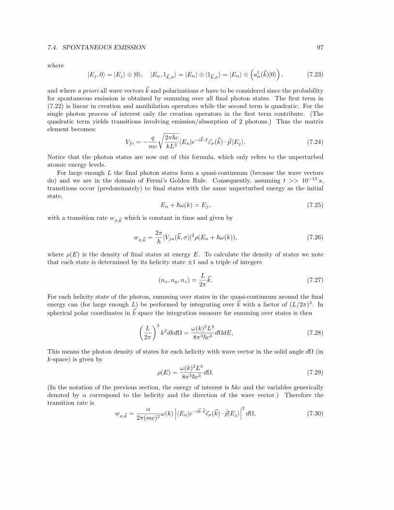
7.4. SPONTANEOUS EMISSION 97
where
|Ej , 0〉 = |Ej〉 ⊗ |0〉, |En, 1~k,σ〉 = |En〉 ⊗ |1~k,σ〉 = |En〉 ⊗(a†σ(~k)|0〉
), (7.23)
and where a priori all wave vectors ~k and polarizations σ have to be considered since the probabilityfor spontaneous emission is obtained by summing over all final photon states. The first term in(7.22) is linear in creation and annihilation operators while the second term is quadratic. For thesingle photon process of interest only the creation operators in the first term contribute. (Thequadratic term yields transitions involving emission/absorption of 2 photons.) Thus the matrixelement becomes:
Vfi = − q
mc
√2π~ckL3
〈En|e−i~k·~x~εσ(~k) · ~p |Ej〉. (7.24)
Notice that the photon states are now out of this formula, which only refers to the unperturbedatomic energy levels.
For large enough L the final photon states form a quasi-continuum (because the wave vectorsdo) and we are in the domain of Fermi’s Golden Rule. Consequently, assuming t >> 10−15 s,transitions occur (predominately) to final states with the same unperturbed energy as the initialstate,
En + ~ω(k) = Ej , (7.25)
with a transition rate wσ,~k which is constant in time and given by
wσ,~k =2π
~|Vjn(~k, σ)|2ρ(En + ~ω(k)), (7.26)
where ρ(E) is the density of final states at energy E. To calculate the density of states we notethat each state is determined by its helicity state ±1 and a triple of integers
(nx, ny, nz) =L
2π~k. (7.27)
For each helicity state of the photon, summing over states in the quasi-continuum around the finalenergy can (for large enough L) be performed by integrating over ~k with a factor of (L/2π)3. In
spherical polar coordinates in ~k space the integration measure for summing over states is then(L
2π
)3
k2dkdΩ =ω(k)2L3
8π3~c3dΩdE, (7.28)
This means the photon density of states for each helicity with wave vector in the solid angle dΩ (ink-space) is given by
ρ(E) =ω(k)2L3
8π3~c3dΩ. (7.29)
(In the notation of the previous section, the energy of interest is ~kc and the variables genericallydenoted by α correspond to the helicity and the direction of the wave vector.) Therefore thetransition rate is
wσ,~k =α
2π(mc)2ω(k)
∣∣∣〈En|e−i~k·~x~εσ(~k) · ~p|Ej〉∣∣∣2 dΩ, (7.30)
98 CHAPTER 7. SPONTANEOUS EMISSION
where α = q2/~c (with q being the magnitude of the electron charge) is the fine structure constant.Notice that this result is independent of the precise value of L; we only need it to be sufficientlylarge.5
7.4.2 Electric dipole transitions
It only remains to deal with the matrix element in (7.30). Fortunately for me, this matrix element isfrequently treated in courses on quantum mechanics and a standard approximation to it is available.The idea is as follows. Because the transition is “energy conserving”, the wavelength of the emittedphoton is related to the change in atomic energy level in the usual way. It is on the order of∼ 10−7m. On the other hand, the position space wave functions being integrated in the matrixelement are non-negligible only out to the Bohr radius or so, say 10−10m. Consequently, theexponent in (7.30) can be neglected in a first approximation:
wσ,~k ≈α
2π(mc)2ω(k)
∣∣∣〈En|~εσ(~k) · ~p|Ej〉∣∣∣2 dΩ, (7.31)
It is now possible to calculate the matrix element explicitly, but it is useful to first put the resultin a more illuminating form via the identity
~p =m
i~[~x, H0]. (7.32)
Replacing the momentum with the commutator, and then taking advantage of the fact that thematrix elements are with respect to eigenvectors of H0, we get
wσ,~k ≈α
2πc2ω(k)3
∣∣∣〈En|~εσ(~k) · ~x|Ej〉∣∣∣2 dΩ. (7.33)
The operator q~x represents the electric dipole moment of the atom and the dot-product withthe polarization vector is proportional to the energy of an electric dipole in a uniform electric fieldalong ~εσ(~k). For this reason the transitions which are considered in this approximation are knownas electric dipole transitions. Using the theory of angular momentum, it is well-known that theelectric dipole matrix element is non-vanishing only when certain selection rules for the differencein angular momentum values, ∆l, ∆m, are satisfied. The electric dipole selection rules are
∆l = ±1, ∆m = 0,±1 (7.34)
The relation ∆m = 0, comes from the term involving the z component of the polarization vector~εσ, while it is the x-y components of the polarization which feature when ∆m = ±1.
It is worth pausing to think about this selection rule in terms of conservation of angular momen-tum.6 The Hamiltonian for the system – atom plus photons – is rotationally invariant and thereforethe total angular momentum is conserved. This angular momentum comes from the atomic orbitalangular momentum and the photon’s helicity, which only contributes angular momentum parallelor anti-parallel to its motion. The change in the total angular momentum of the atom, ∆l = ±1,
5Since the typical photon wavelengths which matter for this transition are ∼ 10−7m, any macroscopic box willbe sufficiently large.
6Our discussion will be imperfect because one really needs a relativistic treatment to properly treat the photon’sspin.
7.4. SPONTANEOUS EMISSION 99
is consistent with conservation of total angular momentum and the spin-1 nature of the photon.(Notice that it is possible for the angular momentum of the atom to increase by emission of a pho-ton.) The z component of the total angular momentum is just the sum of the z components of theindividual angular momenta of the atom and photon. If the photon is emitted along the z axis thenits polarization vector is in the x-y plane, whence the selection rule ∆m = ±1 applies, which jibeswith the idea that the component of the photon’s intrinsic angular momentum along the directionof propagation of the photon (in a momentum eigenstate) is ±~. If the photon has polarizationonly along z then it is propagating in the x-y plane and has no intrinsic angular momentum alongz, consistent with the selection rule ∆m = 0.
To get the transition rate in final form we sum over all final photon states. This involves adiscrete sum over polarizations and an integral over wave vector directions. We take care of this asfollows. The absolute value of each component of the matrix element of ~x defines a vector in R3
which I will denote by ~xnj ,
~xnj ≡ |〈En|~x|Ej〉|. (7.35)
Recall that the vectors (~ε1(~k),~ε2(~k),~k/k) form an oriented orthonormal basis in R3. Let θ be the
angle between ~k and ~xnj . Imagine projecting ~xnj into the plane orthogonal to ~k. Let φ be the angleof that projection with respect to ~ε1. We can then write
~xnj = xnj
(cos θ
~k
k+ sin θ cosφ~ε1 + sin θ sinφ~ε2
), (7.36)
so that~ε1 · ~xnj = xnj sin θ cosφ, ~ε2 · ~xnj = xnj sin θ sinφ, (7.37)
and hence ∑σ
∣∣∣〈En|~εσ(~k) · ~x|Ej〉∣∣∣2 = x2nj sin2 θ, (7.38)
where θ is the angle between ~k and ~xnj . To sum over all directions for ~k we can temporarily view
our z axis as being along ~xnj . Then θ is the polar angle of ~k and the solid angle is dΩ = −dφd(cos θ).The integration over photon propagation directions in the matrix element is x2nj multiplied by∫ 2π
0
dφ
∫ 1
−1d(cos θ) sin2 θ =
8π
3. (7.39)
Putting together (7.33), (7.38), and (7.39), the transition rate is given by7
w =4α
3c2ω3x2nj , ω =
|En − Ej |~
. (7.40)
To summarize, a principal effect of coupling a hydrogenic electron (in an excited atomic state) tothe photon field via (7.15) is to cause a transition to a lower energy atomic state with the emissionof a photon. The energy and angular momentum of the emitted photon accounts for the differencebetween the initial and final electron energies and angular momenta. The transition rate is givenby (7.40). Of course this is the standard description of spontaneous emission that you have heard
7This is consistent with [3] and corrects (23.54) in [2].

100 CHAPTER 7. SPONTANEOUS EMISSION
of. It is perhaps enlightening to review how many approximations and idealizations are needed toget this familiar scenario. This result only appears at first order in perturbation theory. We needthe size of the region in which we are working to be sufficiently large (compared to the wavelengthof the emitted photon) to get a quasi-continuum of final photon states. We need the transition timeto be sufficiently long compared to atomic time scales so we can use Fermi’s Golden rule. Finallywe need the emitted photons to have a wavelength much bigger than the Bohr radius so we canuse the electric dipole approximation. If any of these approximations are violated the standardphenomenology of spontaneous emission will not necessarily apply.
7.4.3 Lifetime of 2P → 1S
Let us use (7.40) to calculate the mean lifetime of the 2P state of a hydrogenic atom with respectto decay by spontaneous emission of a single photon. The initial state has the atomic electron inone of its first excited states with non-vanishing angular momentum (n = 2, l = 1,m = 0,±1) andzero photons. The final state has the atomic electron in the ground state (n = 1, l = 0,m = 0)and a photon with energy ~ω(k) = E2 − E1. We need to calculate the matrix element (7.35) in(7.40) then average over the three possible initial states. I will only do the computation for theinitial state in the m = 0 case since the other two cases give the same result thanks to rotationalsymmetry. So, we want the position vector matrix element with respect to the states (7.9) and(7.10). With ~x = (r sin θ cosφ, r sin θ sinφ, r cos θ) we get
〈1, 0, 0|~x|2, 1, 0〉 =
∫ 2π
0
dφ
∫ π
0
dθ
∫ ∞0
dr r2 sin θ ~x
(√Z3
πa3e−Zr/a
)(√Z3
32πa3Zr
acos θe−Zr/2a
)(7.41)
= (0, 0,128√
2
243
a
Z). (7.42)
The other 2 initial states (m = ±1) give the same result up to a phase, so the average – thetransition rate – is given by
w =131072
177147
αa2ω3
Z2c2=
256
6561Z4α5mc
2
~. (7.43)
This is the number of transitions per unit time. The mean lifetime τ is the reciprocal of thistransition rate, τ = 1/w. With
~ = 6.582× 10⁻¹⁶ eV - s, mc2 = 5.110× 10⁵ eV, α = 0.0073 (7.44)
we get
w = 6.280× 10⁸Z4 s−1, τ =1.592× 10⁻⁹
Z4s. (7.45)
The experimental values I found for the lifetime in the case of hydrogen (Z = 1) were
τ = (1.600± 0.004)× 10−9 s, (see reference [9])
τ = (1.60± 0.01)× 10−9 s, (see reference [10])
These measurements agree well with the theoretical value (7.45), particularly when you considerthat we have ignored all kinds of important adjustments to the structure of the atom, for example,spin-orbit coupling (fine structure) and coupling to nuclear spin (hyperfine structure).
7.5. ANOTHER PERSPECTIVE 101
7.5 Another perspective
We have seen that the coupling of an atomic electron to the quantum electromagnetic field leadsto transitions between the (former) stationary states of the system. This point of view is the oneafforded by Dirac’s time-dependent perturbation theory which approximates the time dependence ofthe solutions of the Schrodinger equation in terms of the unperturbed (non-interacting) system. Itis interesting to consider the perspective provided by time-independent perturbation theory. Recallthat this is a way to approximate the spectrum of a (time-independent) Hamiltonian in termsof its unperturbed (non-interacting) form.8 As mentioned earlier, the interaction between theelectron and photons renders the original non-interacting stationary states no longer stationary:the interaction changes the Hamiltonian with a concomitant change in the energy eigenvectors.As far as I know, despite the relative simplicity of the model, there is no known formula for thespectrum of the Hamiltonian (7.15). However, we can consider the approximation of the spectrumvia time-independent perturbation theory.
Let me remind you of the salient results of time-independent perturbation theory. If the Hamil-tonian H takes the form
H = H0 + V (7.46)
with a suitably small perturbation V , the eigenvalues En and eigenvectors |En〉 of H can be sys-tematically approximated in terms of those for H0, which are denoted by E0
n, |E0n〉. To first order
in the perturbation we have (for non-degenerate eigenvalue E0n)
En ≈ E0n + 〈E0
n|V |E0n〉, (7.47)
|En〉 ≈ |E0n〉+
∑k 6=n
〈E0k|V |E0
n〉E0n − E0
k
|E0k〉, (7.48)
where the sum over k is a sum over a basis of unperturbed energy eigenvectors excluding the one with(non-degenerate) eigenvalue E0
n. (The approximate energy eigenvector has not been normalized. )There is a bit more to the story, but this will serve for the present discussion.
Let us imagine applying (7.47) and (7.48) to obtain a more accurate description of the groundstate of hydrogen. Recall that the unperturbed stationary states are given by (7.11), which arestates where the electron is in one of the usual hydrogenic energy levels with various numbersof photons in various stationary states. In particular, the unperturbed ground state is the usualground state of hydrogen with zero photons: |ψ100〉⊗|0〉 and the unperturbed ground state energy is−13.6 eV. What becomes of this ground state when the interaction with photons is accounted for?Evidently, the ground state is “dressed” with contributions from the (unperturbed) excited atomicstates and various photon states. The contribution of these “virtual” states to the “dressing” ofthe ground state is (to first order) determined by the matrix element of V between the groundstate and the other unperturbed stationary states. For example, much as we saw earlier, the matrixelement of the ~A · ~p term in the Hamiltonian will, in the electric dipole approximation, dress theground state with virtual excited hydrogenic states (where l = 1 and m = ±1, 0) and virtual photonstates (with any energy-momentum and polarization). The A2 term in the Hamiltonian will dressthe ground state with virtual excited hydrogenic states containing two virtual photons.9 So, theprobability distributions for observables like the position and momentum of the electron will receive
8The relation between these two approximation schemes can be obtained via (2.102).9The ~A · ~p term will also contribute two photon states at second order in the perturbation.

102 CHAPTER 7. SPONTANEOUS EMISSION
small corrections which render them much more intricate than in the non-interacting theory. It iseasy to see that the first-order correction to the ground state energy itself vanishes, although it willreceive (very small) corrections at the next order in perturbation theory.
One often uses a very picturesque language to describe the state of affairs sketched above. Onesays the true ground state of the atom involves the atomic electron making “virtual transitions”to and from the unperturbed ground state, emitting and absorbing a cloud of “virtual photons”.Of course, one cannot take this language too literally: the virtual processes do not conserve energyand are, in any case, unobservable as real dynamical processes (in contrast to, e.g., spontaneousemission of a real photon). Still, this way of speaking does give some life to the formula (7.48). Youcan read more about all this in reference [11].
7.6 Problems
1. Consider a “2-state system”, that is, a system with a two-dimensional Hilbert space. Supposethe Hamiltonian is
H = H0 + V , H0 =
(E1 00 E2
), V =
(0 γγ 0
)(7.49)
Solve the Schrodinger equation assuming the initial state is the eigenstate of H0 with eigen-value E1. Find the probability that the system is in the eigenstate of H0 with eigenvalue E0 attime t. Show how the formula (7.17) defines an approximation to this transition probability.
2. Show that the term quadratic in ~A in H is responsible for atomic transitions involving emissionor absorption of 2 photons.
3. An atom in the presence of electromagnetic radiation can emit photons by stimulated emission.Consider a transition from an atomic state |Ej〉 in the presence of N photons with polarization
σ and wave vector ~k to a state |En〉 in the presence of N + 1 photons with polarization σ and
wave vector ~k. Calculate the analog of the matrix element (7.24). Show that for large N thissame matrix element can be obtained by applying time dependent perturbation theory justto the hydrogenic atom in the presence of a suitable classical electromagnetic field.
4. Show that a hydrogenic transition 2S → 1S by spontaneous emission of a single photon isforbidden to first-order in perturbation theory.
5. Calculate the transition rates for |2, 1,±1〉 → |1, 0, 0〉 and show that they give the same resultsas we calculated for |2, 1, 0〉 → |1, 0, 0〉.
6. The parity of a quantum state of a particle refers to its behavior under the transformation~x → −~x. If a state is unchanged by this transformation it is said to have even parity. Ifit changes sign under this transformation it is said to have odd parity. Show that electricdipole transitions necessarily change the parity (even ↔ odd) of the unperturbed hydrogenicstationary state. Show that |1, 0, 0〉 has even parity and |2, 1, 0〉 has odd parity.

Chapter 8
Epilogue
The scope of this text has been intentionally rather modest. Indeed, most of the preceding resultswere already in place by the 1930’s. Needless to say, a lot has happened to quantum field theorysince then. Let me very briefly mention some of the salient results.1
The principal conclusion of decades of experimental and theoretical work in the 20th centurywas that everything can be described by quantum fields. Matter is described in terms of fermionicfields while the (non-gravitational) interactions between matter fields are described by “non-Abeliangauge fields”, which are bosonic fields incorporating and generalizing the quantum electromagneticfield. The proper framework for doing all this is the “standard model” of particle physics. Thestandard model builds all of the known matter from quark fields and lepton fields. Quantum gaugefields represent the strong and electroweak interactions amongst the matter. Finally the standardmodel includes a spin-0 (scalar) field, known as the Higgs field, which allows for particle excitationsof various fields to acquire mass in appropriate “low energy” limits.
The majority of predictions of the standard model are obtained via perturbation theory and arethus phrased in terms of interactions between various particles. But some of the more profoundphysical results are best thought of in terms of the quantum fields themselves. I have in mind,for example, the emergence of the renormalization group as a way of understanding and relatingphysics at disparate length scales. It is perhaps also worth mentioning that some observed physicaleffects, e.g., the Casimir effect, are normally understood purely in terms of quantum fields – thiseffect occurs in the vacuum state – and the particle point of view is simply not relevant.
The gravitational interaction is a good deal more complicated from the point of view of quantumfield theory. Classically, gravitation is described in terms of the curvature of spacetime via Einstein’sgeneral theory of relativity. There are two levels of sophistication one can use when incorporatinggravitational effects in quantum field theory. The simplest approach is to try to define quantum fieldtheory in a curved spacetime. This allows one to incorporate the influence of, say, the cosmologicalexpansion, or the event horizon of a black hole, on particle physics. The constructions used inthis text tacitly took advantage of the properties of flat spacetime. Some of these constructionsgeneralize to a curved spacetime and some do not. Consequently some qualitatively new featuresarise when incorporating gravitation in this way One of the most striking results of extendingquantum field theory to curved spacetimes is that the notion of “particles” becomes ambiguous.
1I don’t pretend to give a comprehensive – or even objective – summary; the choice of ideas to emphasize and mycharacterization of them is based upon my personal prejudices.
103

104 CHAPTER 8. EPILOGUE
Depending upon the gravitational field, different observers need not agree on the particle content ofthe state of a quantum field. Physical manifestations of this phenomenon are particle production byan expanding universe and “Hawking radiation” from black holes. Quantum field theory in curvedspacetime underscores the primacy of the notion of quantum field over the notion of particle [12]
Quantum field theory in curved spacetime is designed to treat gravitation classically and every-thing else quantum mechanically. There are a number of reasons to believe that this frameworkcannot provide the ultimate description of gravitation. For example, there exist several argumentssuggesting that to couple a classical system to a quantum system in this way is at best a limitedapproximation – and ultimately inconsistent. A more ambitious attempt to incorporate gravita-tion into the framework of quantum field theory is then to view gravitation itself as a quantumphenomenon.
Starting from Einstein’s theory approximated near flat spacetime, it is possible to construct aquantum theory of a non-interacting gravitational field, quite analogous to what we did with theelectromagnetic field. This quantum gravitational field has massless helicity-2 particle excitations,usually called “gravitons”. In perturbation theory one can build the interaction of gravitons withparticles and recover (perturbatively) the classical gravitational interaction of Einstein’s theory.Challenges occur when one tries to go beyond this point and incorporate genuine quantum effects.Technically, the perturbation expansion only defines the quantum gravity theory in conjunctionwith measurement of an infinite number of coupling constants – the theory is “non-renormalizable”.Alternatively, one still needs to find a high energy/short distance quantum field theory to “complete”the quantum field theory which is approximated by Einstein gravity at sufficiently large distancescales. Conceptual problems also arise from the fact that the spacetime geometry in a putativequantum field theory of gravity should somehow be undergoing quantum fluctuations. Normally,the (classical) spacetime geometry is used to build and interpret a quantum field theory, so itbecomes problematic to construct a quantum field theory of the spacetime geometry itself. Thechallenges inherent in devising a quantum description of the gravitational interaction represent, inmany ways, the principal problem of theoretical physics. Without some compelling guidance fromexperiment, it is likely to remain an open problem for some time to come.
Bibliography
[1] P. A. M. Dirac, The Principles of Quantum Mechanics, Oxford Science Publications (1958).
[2] E. Merzbacher, Quantum Mechanics, John Wiley & Sons (1998).
[3] J. Sakurai, Advanced Quantum Mechanics, Addison-Wesley (1982).
[4] A. Einstein, B. Podolsky, N. Rosen, “Can Quantum-Mechanical Description of Physical Realitybe Considered Complete?” Phys. Rev. 47, 777–780 (1935).
[5] C. G. Torre, Introduction to Classical Field Theory, https://digitalcommons.usu.edu/lib mono/3/(2017).
[6] T. Newton and E. Wigner, “Localized States for Elementary Systems”, Rev. Mod. Phys. 21,845 (1949).
[7] A. S. Wightman, “On the Localizability of Quantum Mechanical Systems”, Rev. Mod. Phys.34, 845 (1962).
[8] T. Jordan, J. Math. Phys 19, 1382 (1978).
[9] W. Bickel and A. Goodman, Phys. Rev. 148, 1 (1966).
[10] E. Chupp, L. Dotchin, and D. Pegg, Phys. Rev. 175 44 (1968).
[11] R. Passante and E. Power, Phys. Rev. A 35, 188 (1987).
[12] P. C. W. Davies, “Particles Do Not Exist,” in Quantum Theory Of Gravity, 66-77 (AdamHilger, 1984).
105


![A short introduction to the quantum formalism[s] · 2012-11-27 · A short introduction to the quantum formalism[s] François David Institut de Physique Théorique CNRS, URA 2306,](https://static.fdocuments.in/doc/165x107/5eb322ab531be317e03273b7/a-short-introduction-to-the-quantum-formalisms-2012-11-27-a-short-introduction.jpg)