What Influences the Relative Proportion of
195
I What Influences the Relative Proportion of ‘Rigid Rotation’ Versus ‘Non-Rigid Deformation’ in a Bistable Stroboscopic Motion Display. Irene Rui Chen A thesis submitted in partial fulfillment of the requirements for the degree of Doctor of Philosophy School of Architecture, Design and Planning University of Sydney 2018
Transcript of What Influences the Relative Proportion of

I
What Influences the Relative Proportion of
‘Rigid Rotation’ Versus ‘Non-Rigid Deformation’
in a Bistable Stroboscopic Motion Display.
Irene Rui Chen
A thesis submitted in partial fulfillment of the requirements for the degree
of Doctor of Philosophy
School of Architecture, Design and Planning
University of Sydney
2018

II
Statement of Originality
This is to certify that:
I. The intellectual content of this thesis is the product of my own
work towards the Doctor of Philosophy Degree
II. Due acknowledgement has been made in the text to all other
material used
III. This thesis does not exceed the word length of this degree.
IV. No part of this work has been used for the award of another degree
V. This thesis meets research code of conduct requirements of the
University of Sydney’s Human Research Ethics Committee
(HREC), ethics reference number: 2013/562.
Name: Irene Rui Chen

III
Abstract
When observers are presented with a bistable stroboscopic display of an object that
appears to transform over time in three-dimensional (3D) space, the dominance of one
percept over another is influenced both by stimulus parameters and by cognitive factors.
Two experiments were designed to reveal which of several manipulated variables
influence most strongly which of two responses is more often observed, one being
termed ‘Rigid Rotation’ and the other termed ‘Non-rigid Deformation.’ These two
responses were clearly distinguished when drawings of a 3D rectangular box were
presented stroboscopically in a two-frame animation with precise control over the
Interstimulus Interval (ISI). In the first experiment, the relative dominance of the ‘Rigid
Rotation’ response was reduced by changing the colour of one surface of the
rectangular box in a manner that was inconsistent with the rotation of the box. Similarly,
the relative dominance of the ‘Non-rigid Deformation’ response was reduced by
changing the colour of one surface of the rectangular box in a manner that was
inconsistent with deformation of the box. In the second experiment, the changes in the
relative dominance of the competing motion percepts were observed after prolonged
viewing of four different adapting stimuli. The adaptation aftereffects were shown to
depend more upon the Interstimulus Interval (ISI) of the stroboscopic display of the
adapting stimulus than upon what motion was reportedly ‘seen’ during the viewing of
the adapting stimulus. Ultimately, the adaption aftereffect revealed that the relative
dominance of the two movement percepts was affected most strongly by the
manipulation of a single temporal variable – the ISI. Nonetheless, the results of the
first experiment confirmed the influence of surface colour variations on ‘Rigid Rotation’
versus ‘Non-rigid Deformation’ responses.

IV
Acknowledgements
I would like to extend my heartfelt gratitude to all those who have given assistance,
encouragement and support throughout my PhD candidature.
First and foremost, I would like to express my sincere appreciation to my supervisor, Associate
Professor William L. Martens, for providing me with his expert direction, guidance and support
through every stage of the thesis with concepts, suggestions, and criticisms over the last few
years. Furthermore, I would like to express my gratitude to my copy editor Dr. Cherry Russell
for reading, editing and commenting on my countless drafts. Without their contribution
completion of this thesis would not have been possible.
Secondly, special recognition to Professor David Alais in the department of psychology,
University of Sydney, for providing his valuable advice and assistance during the early stage
of the research.
Thanks are also due to Associate Professor Wendy Davis for allowing me to use her lighting
lab to conduct my experiments. Many thanks to the observers who voluntarily participated in
all the experiments; without them the data collection would not have been possible.
Special thanks to Dr Jennifer Gamble, Mr Stephen Broune and Mr David Haley, Mr Phil Davis,
Mr Gary Jannese, and Dr Ali Khoddami, all of whom had faith in me and provided their support
and comfort throughout this long journey.
I would also like to extend my gratitude to various University of Sydney staff members,
especially Associate Professor Paul Jones, Professor Richard de Dear, Ms Violeta Birks and
Leslie George who offered understanding and support throughout my candidature.
Also, I wish to acknowledge the support and encouragement from the research students in my
office: Nickash Singh, Dheyaa Ali Hussein and Mansour Alulayet. Thank you for the
discussion, help, encouragement and laughs.
Special thanks to my oldest friend Mr Clive Evatt for his special humour and sarcasm that
strengthened my determination to complete this long journey.

V
Last but not least, infinite thanks to my parents for their generous support, prayers and love
throughout the struggles of this amazing journey, especially my mother for sharing the burden
of caring for my sick father despite her own health issue, so I could work through the last stage
of my thesis. This thesis is dedicated to them.
Table of Contents:
I
Table of Contents
Chapter 1: introduction ......................................................................................................... 1
1.1 Multistable Perception .......................................................................................................... 2
1.1.1 Still Images ................................................................................................................... 2
1.1.2 Stroboscopically Displayed Images .............................................................................. 5
1.2 Sensory Variables versus Cognitive Variables ................................................................... 7
1.3 Pre-attentive Processing and the Two-Process Model ..................................................... 11
1.4 Early Work on Apparent Motion ...................................................................................... 16
1.4.1 The Motion After-effect (MAE) ................................................................................. 18
1.4.2 Relation between 2D and 3D Structure in Motion ...................................................... 20
1.4.3 Recognition-by-Components and the Correspondence Problem ................................ 23
1.5 Perceptual Cycle .................................................................................................................. 27
1.5.1 Hypothesis .................................................................................................................. 29
1.6 Current Understanding of the Topic ................................................................................. 33
CHAPTER 2: LITERATURE REVIEW ......................................................................... 35
2.1 Multistable Apparent Motion ............................................................................................. 35
2.1.1 The Ternus Display .............................................................................................. ….36
2.2 Perceptual Organisation ..................................................................................................... 37
2.2.1 Central versus Peripheral Processes ......................................................................... 46
2.3 Studies of Motion After-effect (MAE) ............................................................................... 49
2.4 Association Field .................................................................................................................. 53
Table of Contents:
II
2.5 The Rigidity Assumption .................................................................................................... 60
CHAPTER 3: RESEARCH METHODS ........................................................................... 63
3.1 Methods Common to the Two Experiments ................................................................... 63
3.2 Methodological Differences between the Two Experiments .......................................... 63
3.3 Methods .............................................................................................................................. 65
3.3.1 Observers .................................................................................................................. 65
3.3.2 Design ....................................................................................................................... 65
3.3.3 Stimulus generation and presentation ....................................................................... 66
3.3.3.1 Laboratory environment and apparatus………………………………………………………….66
3.3.3.2 Graphic image generation for rigid rotation and non-rigid deformation……………………67
3.3.3.3 Cycle duration……………………………………………………………………………………… .69
3.4 Procedure .......................................................................................................................... .70
3.5 Recording Methods and Results Calculations…………………………………………..73
CHAPTER 4: Experiment 1 ............................................................................................... 75
4.1 Method ............................................................................................................................... .75
4.1.1 Observers .................................................................................................................. 75
4.1.2 Design ....................................................................................................................... 75
4.1.3 Stimuli....................................................................................................................... 79
4.2 Procedure ........................................................................................................................... 80
4.3 Results ................................................................................................................................ 80
4.3.1 Distribution of proportional responses of rigid rotation ........................................... 82
Table of Contents:
III
4.3.2 Proportion of rigid rotation for the thin sponge under three conditions ................... 83
4.3.3 Proportion of rigid rotation for the fat sponge under three conditions ..................... 84
4.3.4 Mean inter-observer correlation: Results for 14 observers for the fat sponge condition
........................................................................................................................................... 85
4.3.5 Parametric Analysis of Proportions, Including Curve Fitting .................................. 89
4.3.6 Z-scores..................................................................................................................... 92
4.3.7 Fat sponge ................................................................................................................. 92
4.3.8 Thin sponge .............................................................................................................. 94
4.4 Results from ANOVA ....................................................................................................... 95
4.5 Discussion ........................................................................................................................... 95
CHAPTER 5: Experiment 2 ............................................................................................ 100
5.1 Introduction ....................................................................................................................... 100
5.2 Methods .............................................................................................................................. 101
5.2.1 Subjects……………………………………………………………………………..101
5.2.2 Design………………………………………………………………………………101
5.2.3 Stimuli……………………………………………………………………………...103
5.2.4 Pilot study…………………………………………………………………………..105
5.3 Results…………………………………………………………………………………….106
5.3.1 Adapting stimuli………………………………………………………………….. 107
5.3.2 Testing stimuli……………………………………………………………………. 109
5.3.3 Analysis using a generalised linear mixed model………………………………....118
Table of Contents:
IV
5.3.3.1 ISI levels……………………………………………………………………………………120
5.3.3.2 Adaptation………………………………………………………………………………….121
5.3.3.3 Observer…………………………………………………………………………………....122
CHAPTER 6: DISCUSSION AND CONCLUSION ...................................................... 123
6.1 Discussion………………………………………………………………………………...123
6.1.1 Experiment 1: Form and Surface Colour………………………………………….123
6.1.2 Experiment 2: Adaptation…………………………………………………………127
6.1.3 Comparison with Results from Other Studies……………………………………. 129
6.2 Conclusion .......................................................................................................................... 134
6.3 Future Work………………………………………………………………………………135
CHAPTER 7: REFERENCES AND BIBLIOGRAPHY................................................ 138
7.1 References ..................................................................................................................... 138
7.2 Bibliography…………………………………………………………………………...145
CHAPTER 8: APPENDIX ................................................................................................ 159
8.1 Participation Information Statement .............................................................................. 159
8.2 Participation Information Form ...................................................................................... 163
8.3 Participant Consent Form ................................................................................................ 164
8.4 Instruction Sheet................................................................................................................ 168
8.5 Feedback and Post-evaluation .......................................................................................... 174
8.6 Hierarchical Loglinear Analysis of Combined Data in Output 4way Table ................ 176
8.7 Thesis Website……………………………………………………………………………..179
List of Figures:
i
List of Figures
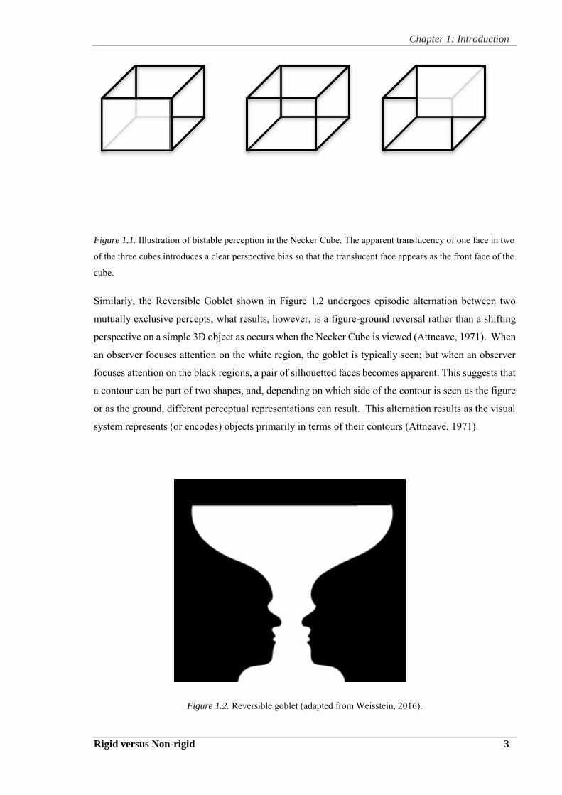
Figure 1.1. Illustration of bistable perception in the Necker Cube. The apparent translucency of one
face in two of the three cubes introduces a clear perspective bias so that the translucent face appears
as the front face of the cube. ................................................................................................................. 3
Figure 1.2. Reversible goblet (adapted from Weisstein, 2016). ........................................................... 3
Figure 1.3. Horse and frog (Dean, 2006). ............................................................................................. 4
Figure 1.4. An old woman and a young girl (Dean, 2006). .................................................................. 4
Figure 1.5. Time structure of a two-frame animation sequence. .......................................................... 5
Figure 1.6. The left panel shows two frames of a stroboscopic display (separated by a blank field for
the ISI) presenting three dots, the middle two of which are always in the same position (as indicated
by the vertical dashed lines). The right panel shows two possible apparent motion percepts that most
observers perceive, in relative proportions that depend on the ISI (shown to be long or short in the
narrow middle panel). These competing apparent motion percepts have been called Group Motion (in
which the three dots move together laterally in a group) and Element Motion (in which the leftmost of
the three dots appears to jump over the two in the middle to come to rest at the rightmost
position). Which perception dominates the other depends on whether the value of the ISI is relatively
longer or shorter than a threshold value, typically around 50 ms. ...................................................... ..6
Figure 1.7. Illustration of how speedlines can give a compelling sense of motion to a still image
(taken from George Herriman’s “Krazy Kat,” 1913)............................................................................ 8
Figure 1.8. (a): Speedlines bias perception towards rigid rotation; (b): Speedlines bias perception
towards non-rigid rotation ........................................................................................................................ 9
Figure 1.9. A graphic interpretation by Verstraten (2015) regarding the experimental setup reported
by Sigmund Exner (1887) in his paper entitled “Einige Beobachtungen über Bewegungsnachbilder”
(Some Observations on Movement After-effects), specifically picturing the set-up assumed for his
Experiment 7 (appearing in Verstraten’s Illustrated Translation with Commentary). ....................... 11
List of Figures:
ii
Figure 1.10. A pair of isosceles triangles appears in the 1st frame; the triangle on the right disappears
when the frames are viewed at short ISI. At a longer ISI the triangle on the right rotates out of the
frontoparallel plane through a 180o angle and terminates at the position of the triangle on the left (i.e.
it lands on top of the triangle on the left). ........................................................................................... 13
Figure 1.11. Left panel: Experimental results reported by Pantle and Picciano (1976), replotted here
to show a comparison in responses between binocular and dichoptic viewing of the three dots in the
Ternus illusion. Right panel: Experimental results reported by Gerbino (1981), replotted here to
show a comparison in responses between monoptic and dichoptic viewing of the triangular display
illustrated in Figure 1.8. ...................................................................................................................... 14
Figure 1.12. The four Kopfermann “cubes” redrawn (taken from Kopfermann, 1930). .................... 21
Figure 1.13. The wire “helix” (a) in frontal view and (b) in top-down view (adapted from Wallach
and O’Connell, 1953). ......................................................................................................................... 22
Figure 1.14. One non-accidental relation (adapted from Biederman, 1987) ...................................... 24
Figure 1.15. Some non-accidental relations in a rectangular box. ...................................................... 25
Figure 1.16. (a) Non-rigid deformation frame (b) Rigid rotation frame ...................... 25
Figure 1.17. The outcome for each vertex as a result of the two kinds of transformation of the
rectangular box from Frame 1 to Frame 2, where each vertex is identified by a frame number and a
letter that is attached in order to underscore what happens to each vertex through the transformations
(moving through either a deformation or a rotation). Note that some vertices that are visible in Frame
1 will become not visible (NV) in Frame 2. ....................................................................................... 26
Figure 1.18. The perceptual cycle (adapted from Neisser, 1978) ....................................................... 27
Figure 1.19. (a) Fat sponge. (b) Thin sponge. ................................................................................... 30
Figure 1.20. Rectangular box with green surface ............................................................................... 30
Figure 1.21. Green-shifting to the side in a manner consistent with object rotation for both fat and
thin sponges when compared to Figure 1.20. ...................................................................................... 30
List of Figures:
iii
Figure 2.1. A Ternus Display study by Dodd et al. (2005)…..……………………………………37
Figure 2.2. Diagram showing unambiguous motion in the surround with single dots moving along the
horizontal axis, presented simultaneously with an ambiguous bistable display in the centre that could
be seen as rotating in either direction (in 90-degree steps)………………………………………...38
Figure 2.3. Two possible motions perceived in the central region of a bistable display in which the
motion in the surrounding field is unambiguous (this drawing is a modified version of the art
presented in Ramachandran and Anstis, 1985). .................................................................... ………39
Figure 2.4. The mean percentages of group movement responses as a function of ISI from 10ms to
80ms with the parameter between the curves being the frame duration values, which were set to
400ms, 200ms and 100ms. ................................................................................................................ 41
Figure 2.5. The mean percentages of group movement responses as a function of cycle duration from
100ms to 500ms with the parameter between the curves being the frame duration values, which were
set to 400ms, 200ms and 100ms. ...................................................................................................... 42
Figure 2.6. Ambiguous stimuli presenting two types of apparent motion: rigid rotation (left pair of
frames) versus non-rigid deformation (right pair of frames). Both pairs illustrate the connection over
time between the local graphical components in association with each type of motion that observers
might experience when presented with these pairs of frames of rectangular box stimuli which, when
looped with varying ISI, form animations that can be perceived in the two identified ways………45
Figure 2.7. Binocular and dichoptic conditions for the two frames of a stroboscopic display in which
dots can be seen either in group motion (for both eyes or for an individual eye) or in element motion
(only for both eyes), depending on whether value of the ISI is relatively longer or shorter. ............ 47
Figure 2.8. (a) Experiment one. ....................................................................................................... 50
Figure 2.8. (b) Experiment two…………………………………………………………….............51
Figure 2.8. (c) Experiment two…………………………………………………………….............52
Figure 2.9. The right column of graphs shows the percepts that result when viewing the four types of
stimuli shown in the left column (Alais and Lorenceau, 2002). ....................................................... 53
Figure 2.10. The associated field (adapted from Field et al., 1993). ................................................ 54
List of Figures:
iv
Figure 2.11. Stimulus for experiment 3 (Alais and Lorenceau, 2002). ............................................ 55
Figure 2.12. Pairs of perspective views of a three-dimensional object that were presented
stroboscopically in the study by Shepard and Judd (1976), showing a 60 degree rotation in the picture
plan (left pair) and a 60 degree rotation in depth about a vertical axis (right pair). .......................... 56
Figure 2.13. Left: A sequence of two 2D rectangular objects. Right: A sequence of two 3D
rectangular objects (see text for an explanation regarding the letters, 1a and 2, labelling the corners of
the graphic objects in this figure). ..................................................................................................... 58
Figure 2.14. The three-loop figures used to demonstrate non-rigid motion: (a) without ‘rivets’ at line
intersections; (b) with ‘rivets’ at intersections; (c) with ‘rivets’ at the loop extremities. ................. 61
Figure 3.1.(a). Rigid rotation. ........................................................................................................... 67
Figure 3.1(b). Non-rigid deformation……………………………………………………………...68
Figure 3.2. Three shapes of the rectangular box ............................................................................... 68
Figure 3.3.(a) Focus on orange circle. Figure 3.3.(b) Focus on blue circle. ..................... 70
Figure 3.4. Necker Cube with red fixation point .............................................................................. 71
Figure 3.5.(a) Element motion. Figure 3.5(b). Group motion………………….….72
Figure 4.1. Trial structure of Experiment 1 ...................................................................................... 75
Figure4.2.(a) Green-stationary thin .................................................................................................. 77
Figure 4.2.(b) Green-stationary fat…………………………………………………………………77
Figure 4.2.(c) Green-shift thin……………………………………………………………………..77
Figure 4.2.(d) Green-stationary fat…………………………………………………………………77
Figure 4.2.(e) All-yellow thin……………………………………………………………………....78
Figure 4.2.(f) All-yellow fat………………………………………………………………………...78
Figure 4.3. Ratios and green-stationary for fat and thin sponges ..................................................... 79
Figure 4.4. Green-shifting to the side in a manner consistent with object rotation for both fat and
thin sponges when compared to Figure 4.3 ....................................................................................... 79
List of Figures:
v
Figure 4.5. Monochrome for both fat and thin sponges ................................................................... 80
Figure 4.6. Three conditions for the proportion of rigid rotation for the thin sponge condition ...... 82
Figure 4.7. Three conditions for the proportion of rigid rotation of the fat sponge condition ......... 83
Figure 4.8. Results for 24 observers for the fat sponge condition .................................................... 86
Figure 4.9. Results for 18 observers for the fat sponge condition .................................................... 86
Figure 4.10. Results for 24 observers for the thin sponge ................................................................ 87
Figure 4.11. Results for 17 observers for the thin sponge ................................................................ 87
Figure 4.12. Results for 24 observers for both fat and thin sponges ................................................ 88
Figure 4.13. Results for 21 observers for both fat and thin sponges ................................................ 89
Figure 4.14. Thin sponge means with standard deviations ............................................................... 90
Figure 4.15. Fat sponge means with standard deviations ................................................................. 90
Figure 4.16. Curves fit to the fat sponge Z-scores ............................................................................ 93
Figure 4.17. Curves fit to the thin sponge Z-scores .......................................................................... 94
Figure 4.18. Curves fit to data for the fat vs. thin sponges in the monochrome condition (with no
green side). ........................................................................................................................................ 97
Figure 4.19. Summary of results for Experiment 1 .......................................................................... 99
Figure 5.1. Trial structure of Experiment 2. ................................................................................... 102
Figure Figure 5.2.(a) Unambiguous animation: Rigid rotation ..................................................... 104
Figure Figure 5.2.(b) Unambiguous animation: Non-rigid rotation………………………………104
Figure 5.2.(c) Ambiguous animation: Biased toward rigid rotation……………………………....105
Figure 5.2.(d) Ambiguous animation: Biased toward non-rigid rotation…………………………105
Figure 5.3. Longer inter-stimulus interval ...................................................................................... 107
Figure 5.4. Shortened inter-stimulus interval. ................................................................................ 107
Figure 5.5. Perception of adapting stimulus ................................................................................... 108
List of Figures:
vi
Figure 5.6. Results given prolonged viewing of the two-frame adapting stimulus under two ISI
conditions. Note that the different images within each animation sequence are illustrated by the inset
graphics—those for the No-ISI sequence above, and those for the 160-ms ISI sequence below the
plotted data. .................................................................................................................................. ...110
Figure 5.7. Results given prolonged viewing of the four-frame adapting stimulus with differing
intermediate frame images, but presented with the same ISI across these two conditions. Note that the
different images within each animation sequence are illustrated by the inset graphics—those for the
non-rigid sequence above and those for the rigid sequence below the plotted data………………111
Figure 5.8. No adapting stimulus………………………………………………………………….112
Figure 5.9. Performance in the four-frame adapting conditions shown relative to performance in the
control condition. ............................................................................................................................ 113
Figure 5.10 . Performance in the two-frame adapting conditions shown relative to performance in the
control condition. ............................................................................................................................ 113
Figure 5.11. Log-odds ratio for four-frame adapting stimulus. ...................................................... 114
Figure 5.12. Log-odds ratio for two-frame adapting stimulus. ....................................................... 115
Figure 5.13. The loglinear model: [RI] [RFA] ............................................................................... 116
Figure 5.14. The log odds for rigid rotation responses after adaptation to four different animations. (a)
The relative dominance of rigid rotation (RR) as a function of increasing ISI, without respect to the
adaptation conditions. (b) The relative dominance of rigid rotation (RR) as a function of 4-frame and
2-frame animations. ........................................................................................................................ 118
Figure 5.15. Probability of observing rigid rotation with increasing ISI levels. ............................ 120
Figure 5.16. Probability of subjects observing rigid rotation……………………………………..122

List of Tables
List of Tables
Table 4.1. ANOVA results given Z-scores for the thin sponge ........................................................... 95
Table 4.2. ANOVA results given Z-scores for the fat sponge ............................................................. 95
Table 4.3. Summary of the Fat curve ................................................................................................ 98
Table 4.4. Summary of the Thin curve………………………………………………………..…….98
Table 5.1. The Model by means of Backwards Elimination…………………………………………….119
Table 5.2. Estimated Variance Components………………………………………………………….…..119
Table 5.3. Predicted Values for ISI Levels……………………………………………………….....120
Table 5.4. Adaptation Conditions…………………………………………………………………. 121
Table 5.5. Logit Estimate for the Control and the Four Adapting Conditions………………...……..121
Table 5.6. Results of Variation from 33 Observers………………………………………………………122
Chapter 1: Introduction
Rigid versus Non-rigid 1
CHAPTER 1: INTRODUCTION
The phenomenon of multistability in visual perception has fascinated many researchers. Put simply, it
refers to the fact that a single stimulus, which remains unchanged over time in a strictly physical sense,
nonetheless appears to change over time to an observer. Over the last hundred years or so, a substantial
body of psychophysical research has focussed on the development of simple relationships between
single stimuli and their singular responses. For example, a briefly flashed monochromatic light on a
dark field typically produces a singular sensation for each stimulus. Imagine how perplexing it would
be if a briefly presented visual stimulus appeared one way on half of the occasions on which it was
presented and another way on the other half, with no corresponding change in the stimulus. If there
were no physical variations that could be measured to predict this change in sensation, then the
experimenter would have to look elsewhere for factors that might be causing this change, such as
changes in the cognition of the observer. In effect, such changes may be due to the influence of
cognitive factors that may or may not be readily explained. Another interesting example of
multistability in visual perception is what occurs when viewing simple stroboscopically displayed
stimuli composed of alternating still images which create illusions of visual motion when presented at
suitable rates of alternation. In both of these cases, the role of sensory versus cognitive factors in
determining what is perceived when human observers are presented with single or alternating still
images can potentially be revealed through careful design of experiments in visual perception.
This introductory chapter presents the background to the study. First it describes the phenomenon of
multistability in perception that occurs when viewing particular still images, such as the familiar
Necker Cube; this is followed by a description of multistability in the perception of rapidly alternating
images (i.e. stroboscopically presented pairs of images that produce at least two competing percepts).
This latter phenomenon—the apparent motion that can be perceived in stroboscopically displayed
images—is the focus of the remainder of this introduction.
A key motivation of the present study was to explore the measureable variables that influence how an
observer’s perception can change between two percepts when the same stimulus is presented. An
important question here is whether sensory or cognitive variables have a stronger influence in
determining what observers will perceive when presented with a stroboscopic display. Previous
research has investigated these issues using different perspectives, ranging from Gestalt theory,
through more stimulus-response relations between 2D stimuli and 3D percepts, and recognisation by
components, and more. Building on this early research, the current study investigated both cognitive
and sensory factors involved in multistable perception via a series of experiments to further explore
these fascinating phenomena in which perception is not locked to stimulus in a one-to-one relationship.
Chapter 1: Introduction
Rigid versus Non-rigid 2
1.1 Multistable Perception
1.1.1 Still Images
Our visual perception is not always stable and some pictures contain ambiguous information that can
lead to competing percepts when viewing a single picture. Indeed, perception can be multistable,
switching between two or more percepts even though the physical stimulus (the picture being viewed)
does not change (Attneave, 1971). Such multistability in perception can be observed when viewing
still images or cyclic animations; however, the most familiar examples are probably those associated
with still images.
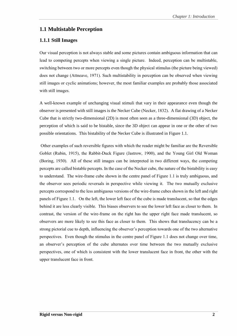
A well-known example of unchanging visual stimuli that vary in their appearance even though the
observer is presented with still images is the Necker Cube (Necker, 1832). A flat drawing of a Necker
Cube that is strictly two-dimensional (2D) is most often seen as a three-dimensional (3D) object, the
perception of which is said to be bistable, since the 3D object can appear in one or the other of two
possible orientations. This bistability of the Necker Cube is illustrated in Figure 1.1.
Other examples of such reversible figures with which the reader might be familiar are the Reversible
Goblet (Rubin, 1915), the Rabbit-Duck Figure (Jastrow, 1900), and the Young Girl Old Woman
(Boring, 1930). All of these still images can be interpreted in two different ways, the competing
percepts are called bistable percepts. In the case of the Necker cube, the nature of the bistability is easy
to understand. The wire-frame cube shown in the centre panel of Figure 1.1 is truly ambiguous, and
the observer sees periodic reversals in perspective while viewing it. The two mutually exclusive
percepts correspond to the less ambiguous versions of the wire-frame cubes shown in the left and right
panels of Figure 1.1. On the left, the lower left face of the cube is made translucent, so that the edges
behind it are less clearly visible. This biases observers to see the lower left face as closer to them. In
contrast, the version of the wire-frame on the right has the upper right face made translucent, so
observers are more likely to see this face as closer to them. This shows that translucency can be a
strong pictorial cue to depth, influencing the observer’s perception towards one of the two alternative
perspectives. Even though the stimulus in the centre panel of Figure 1.1 does not change over time,
an observer’s perception of the cube alternates over time between the two mutually exclusive
perspectives, one of which is consistent with the lower translucent face in front, the other with the
upper translucent face in front.
Chapter 1: Introduction
Rigid versus Non-rigid 3
Figure 1.1. Illustration of bistable perception in the Necker Cube. The apparent translucency of one face in two
of the three cubes introduces a clear perspective bias so that the translucent face appears as the front face of the
cube.
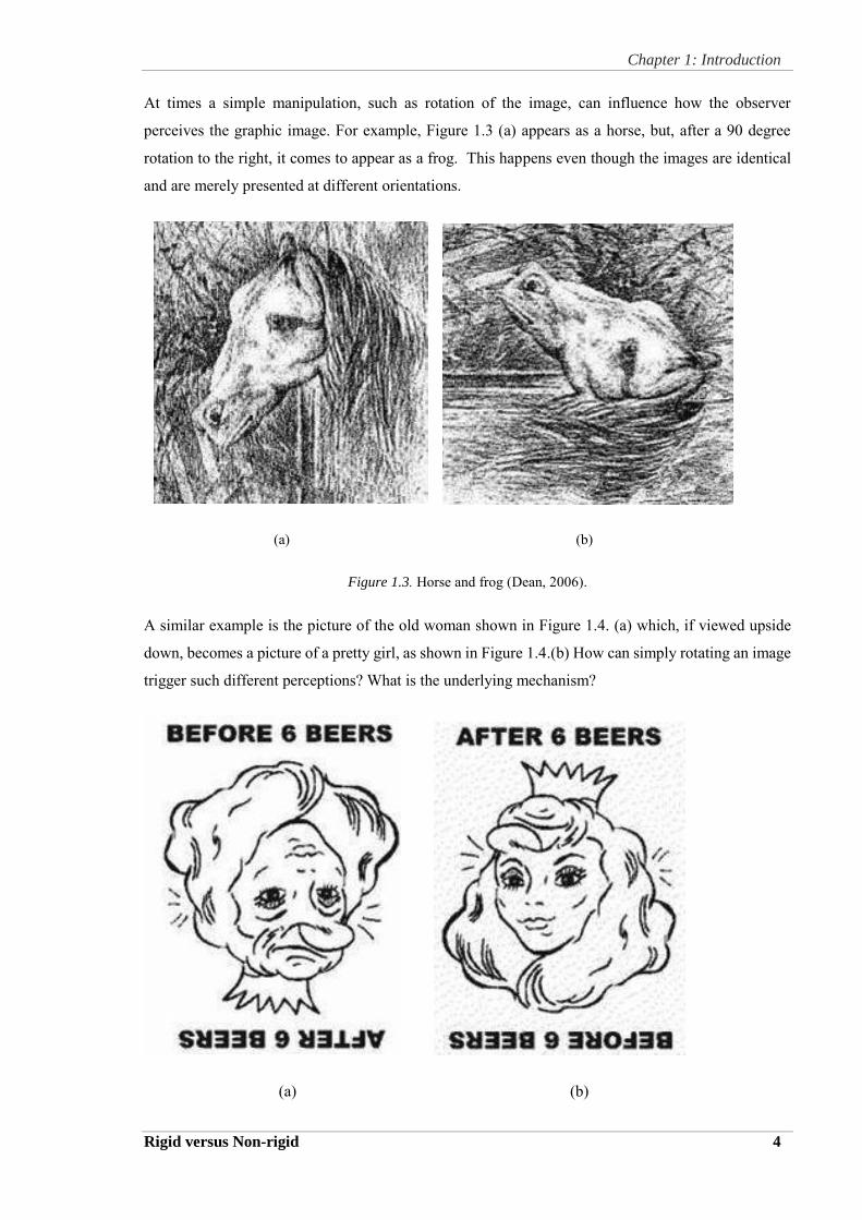
Similarly, the Reversible Goblet shown in Figure 1.2 undergoes episodic alternation between two
mutually exclusive percepts; what results, however, is a figure-ground reversal rather than a shifting
perspective on a simple 3D object as occurs when the Necker Cube is viewed (Attneave, 1971). When
an observer focuses attention on the white region, the goblet is typically seen; but when an observer
focuses attention on the black regions, a pair of silhouetted faces becomes apparent. This suggests that
a contour can be part of two shapes, and, depending on which side of the contour is seen as the figure
or as the ground, different perceptual representations can result. This alternation results as the visual
system represents (or encodes) objects primarily in terms of their contours (Attneave, 1971).
Figure 1.2. Reversible goblet (adapted from Weisstein, 2016).
Chapter 1: Introduction
Rigid versus Non-rigid 4
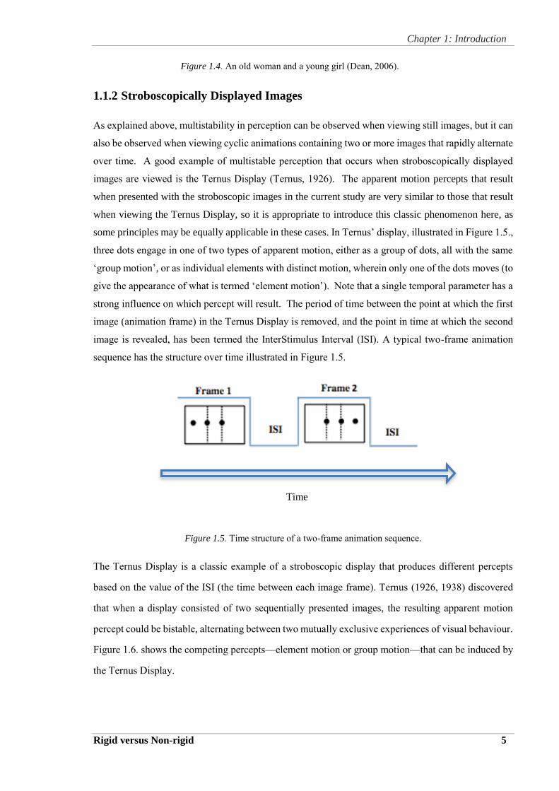
At times a simple manipulation, such as rotation of the image, can influence how the observer
perceives the graphic image. For example, Figure 1.3 (a) appears as a horse, but, after a 90 degree
rotation to the right, it comes to appear as a frog. This happens even though the images are identical
and are merely presented at different orientations.
(a) (b)
Figure 1.3. Horse and frog (Dean, 2006).
A similar example is the picture of the old woman shown in Figure 1.4. (a) which, if viewed upside
down, becomes a picture of a pretty girl, as shown in Figure 1.4.(b) How can simply rotating an image
trigger such different perceptions? What is the underlying mechanism?
(a) (b)
Chapter 1: Introduction
Rigid versus Non-rigid 5
Figure 1.4. An old woman and a young girl (Dean, 2006).
1.1.2 Stroboscopically Displayed Images
As explained above, multistability in perception can be observed when viewing still images, but it can
also be observed when viewing cyclic animations containing two or more images that rapidly alternate
over time. A good example of multistable perception that occurs when stroboscopically displayed
images are viewed is the Ternus Display (Ternus, 1926). The apparent motion percepts that result
when presented with the stroboscopic images in the current study are very similar to those that result
when viewing the Ternus Display, so it is appropriate to introduce this classic phenomenon here, as
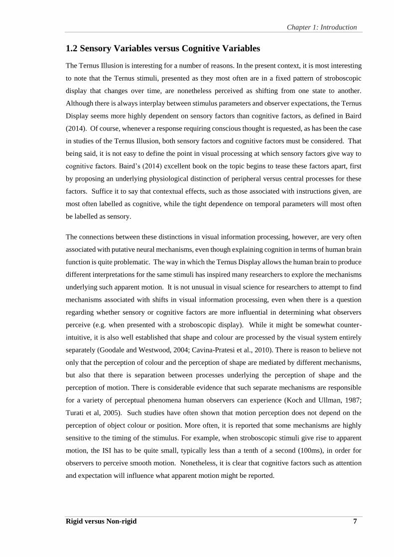
some principles may be equally applicable in these cases. In Ternus’ display, illustrated in Figure 1.5.,
three dots engage in one of two types of apparent motion, either as a group of dots, all with the same
‘group motion’, or as individual elements with distinct motion, wherein only one of the dots moves (to
give the appearance of what is termed ‘element motion’). Note that a single temporal parameter has a
strong influence on which percept will result. The period of time between the point at which the first
image (animation frame) in the Ternus Display is removed, and the point in time at which the second
image is revealed, has been termed the InterStimulus Interval (ISI). A typical two-frame animation
sequence has the structure over time illustrated in Figure 1.5.
Figure 1.5. Time structure of a two-frame animation sequence.
The Ternus Display is a classic example of a stroboscopic display that produces different percepts
based on the value of the ISI (the time between each image frame). Ternus (1926, 1938) discovered
that when a display consisted of two sequentially presented images, the resulting apparent motion
percept could be bistable, alternating between two mutually exclusive experiences of visual behaviour.
Figure 1.6. shows the competing percepts—element motion or group motion—that can be induced by
the Ternus Display.
Time

Chapter 1: Introduction
Rigid versus Non-rigid 6
Figure 1.6. The left panel shows two frames of a stroboscopic display (separated by a blank field for the ISI)
presenting three dots, the middle two of which are always in the same position (as indicated by the vertical
dashed lines). The right panel shows two possible apparent motion percepts that most observers perceive, in
relative proportions that depend on the ISI (shown to be long or short in the narrow middle panel). These
competing apparent motion percepts have been called Group Motion (in which the three dots move together
laterally in a group) and Element Motion (in which the leftmost of the three dots appears to jump over the two
in the middle to come to rest at the rightmost position). Which perception dominates the other depends
on whether the value of the ISI is relatively longer or shorter than a threshold value, typically around 50 ms.
A blank image lasting an adjustable duration was inserted between the first and second frames as the
ISI. As the two frames showing consecutively depend on the duration of the ISI, it was reported that
one of two types of apparent motion could be observed. When the ISI was shorter than 50ms, element
motion was seen most of the time, as shown in Figure 1.6. (bottom). When the ISI was longer than
50ms, group motion was reported more often, as shown in Figure 1.6. (top). However, when the ISI
was around 40-50ms, the bistable appearance could be produced from the Ternus display. Therefore,
the bistable percepts can appear from both still images and cyclic animations.
Chapter 1: Introduction
Rigid versus Non-rigid 7
1.2 Sensory Variables versus Cognitive Variables
The Ternus Illusion is interesting for a number of reasons. In the present context, it is most interesting
to note that the Ternus stimuli, presented as they most often are in a fixed pattern of stroboscopic
display that changes over time, are nonetheless perceived as shifting from one state to another.
Although there is always interplay between stimulus parameters and observer expectations, the Ternus
Display seems more highly dependent on sensory factors than cognitive factors, as defined in Baird
(2014). Of course, whenever a response requiring conscious thought is requested, as has been the case
in studies of the Ternus Illusion, both sensory factors and cognitive factors must be considered. That
being said, it is not easy to define the point in visual processing at which sensory factors give way to
cognitive factors. Baird’s (2014) excellent book on the topic begins to tease these factors apart, first
by proposing an underlying physiological distinction of peripheral versus central processes for these
factors. Suffice it to say that contextual effects, such as those associated with instructions given, are
most often labelled as cognitive, while the tight dependence on temporal parameters will most often
be labelled as sensory.
The connections between these distinctions in visual information processing, however, are very often
associated with putative neural mechanisms, even though explaining cognition in terms of human brain
function is quite problematic. The way in which the Ternus Display allows the human brain to produce
different interpretations for the same stimuli has inspired many researchers to explore the mechanisms
underlying such apparent motion. It is not unusual in visual science for researchers to attempt to find
mechanisms associated with shifts in visual information processing, even when there is a question
regarding whether sensory or cognitive factors are more influential in determining what observers
perceive (e.g. when presented with a stroboscopic display). While it might be somewhat counter-
intuitive, it is also well established that shape and colour are processed by the visual system entirely
separately (Goodale and Westwood, 2004; Cavina-Pratesi et al., 2010). There is reason to believe not
only that the perception of colour and the perception of shape are mediated by different mechanisms,
but also that there is separation between processes underlying the perception of shape and the
perception of motion. There is considerable evidence that such separate mechanisms are responsible
for a variety of perceptual phenomena human observers can experience (Koch and Ullman, 1987;
Turati et al, 2005). Such studies have often shown that motion perception does not depend on the
perception of object colour or position. More often, it is reported that some mechanisms are highly
sensitive to the timing of the stimulus. For example, when stroboscopic stimuli give rise to apparent
motion, the ISI has to be quite small, typically less than a tenth of a second (100ms), in order for
observers to perceive smooth motion. Nonetheless, it is clear that cognitive factors such as attention
and expectation will influence what apparent motion might be reported.

Chapter 1: Introduction
Rigid versus Non-rigid 8
Ross, Badcock and Hayes (2000) showed that form, although processed independently of motion, can
give consistency to what might otherwise appear as incoherent motion. An example of the sort of
incoherent motion to which they refer is given by sequences called Glass patterns (Glass, 1969), in
which some portion of a field of random dots move together in a consistent direction. The ‘global’
pattern for these dots showing coherent motion give rise to a motion percept despite the fact that only
a small percentage of the dots in a given region are joined in that group (for example, as low as 10%).
So, these Glass patterns are built by using a common global rule without coherent motion signals, but
, they produce motion consistent with the global rule for form, rather than the random velocity
components contained within the remainder of the pattern sequence. Similar results were obtained by
Lennie (1998), who suggested that all image attributes, including form and motion, should be
considered together at all stages of visual analysis.
Another example of form influencing motion can be found in the effects of ‘speedlines’ studied by
Burr and Ross (2002), who pointed out that detection of direction of motion is one of the more difficult
tasks for the visual system, which can be aided by static cues. As an example, they present a still
cartoon image taken from George Herriman’s “Krazy Kat” comic, illustrating that speedlines give a
convincing sense of motion to a brick that is tossed at the titular character. As shown in Figure 1.7.,
including a few motion-suggesting speedlines strikes above the character can provides a cue that can
aid in resolving direction ambiguities. Initially it is hard to tell whether the character was moving left
or right, or that the brick was moving, but the speedlines show clearly that the brick is moving upwards
after striking the character. It is natural to conclude that these speedlines influence visual motion
perception.
Figure 1.7. Illustration of how speedlines can give a compelling sense of motion to a still image (taken from
George Herriman’s “Krazy Kat,” 1913).
Chapter 1: Introduction
Rigid versus Non-rigid 9
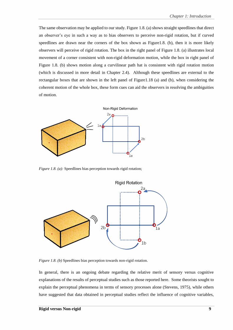
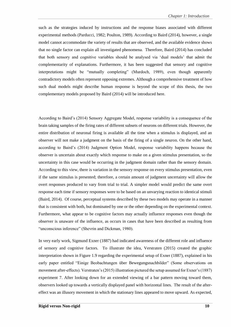
The same observation may be applied to our study. Figure 1.8. (a) shows straight speedlines that direct
an observer’s eye in such a way as to bias observers to perceive non-rigid rotation, but if curved
speedlines are drawn near the corners of the box shown as Figure1.8. (b), then it is more likely
observers will perceive of rigid rotation. The box in the right panel of Figure 1.8. (a) illustrates local
movement of a corner consistent with non-rigid deformation motion, while the box in right panel of
Figure 1.8. (b) shows motion along a curvilinear path hat is consistent with rigid rotation motion
(which is discussed in more detail in Chapter 2.4). Although these speedlines are external to the
rectangular boxes that are shown in the left panel of Figure1.18 (a) and (b), when considering the
coherent motion of the whole box, these form cues can aid the observers in resolving the ambiguities
of motion.
Figure 1.8. (a): Speedlines bias perception towards rigid rotation;
Figure 1.8. (b) Speedlines bias perception towards non-rigid rotation.
In general, there is an ongoing debate regarding the relative merit of sensory versus cognitive
explanations of the results of perceptual studies such as those reported here. Some theorists sought to
explain the perceptual phenomena in terms of sensory processes alone (Stevens, 1975), while others
have suggested that data obtained in perceptual studies reflect the influence of cognitive variables,
Chapter 1: Introduction
Rigid versus Non-rigid 10
such as the strategies induced by instructions and the response biases associated with different
experimental methods (Parducci, 1982; Poulton, 1989). According to Baird (2014), however, a single
model cannot accommodate the variety of results that are observed, and the available evidence shows
that no single factor can explain all investigated phenomena. Therefore, Baird (2014) has concluded
that both sensory and cognitive variables should be analysed via ‘dual models’ that admit the
complementarity of explanations. Furthermore, it has been suggested that sensory and cognitive
interpretations might be “mutually completing” (Murdoch, 1989), even though apparently
contradictory models often represent opposing extremes. Although a comprehensive treatment of how
such dual models might describe human response is beyond the scope of this thesis, the two
complementary models proposed by Baird (2014) will be introduced here.
According to Baird’s (2014) Sensory Aggregate Model, response variability is a consequence of the
brain taking samples of the firing rates of different subsets of neurons on different trials. However, the
entire distribution of neuronal firing is available all the time when a stimulus is displayed, and an
observer will not make a judgment on the basis of the firing of a single neuron. On the other hand,
according to Baird’s (2014) Judgment Option Model, response variability happens because the
observer is uncertain about exactly which response to make on a given stimulus presentation, so the
uncertainty in this case would be occurring in the judgment domain rather than the sensory domain.
According to this view, there is variation in the sensory response on every stimulus presentation, even
if the same stimulus is presented; therefore, a certain amount of judgment uncertainty will allow the
overt responses produced to vary from trial to trial. A simpler model would predict the same overt
response each time if sensory responses were to be based on an unvarying reaction to identical stimuli
(Baird, 2014). Of course, perceptual systems described by these two models may operate in a manner
that is consistent with both, but dominated by one or the other depending on the experimental context.
Furthermore, what appear to be cognitive factors may actually influence responses even though the
observer is unaware of the influence, as occurs in cases that have been described as resulting from
“unconscious inference” (Shevrin and Dickman, 1980).
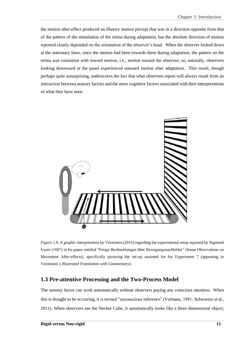
In very early work, Sigmund Exner (1887) had indicated awareness of the different role and influence
of sensory and cognitive factors. To illustrate the idea, Verstraten (2015) created the graphic
interpretation shown in Figure 1.9 regarding the experimental setup of Exner (1887), explained in his
early paper entitled “Einige Beobachtungen über Bewegungsnachbilder” (Some observations on
movement after-effects). Verstraten’s (2015) illustration pictured the setup assumed for Exner’s (1887)
experiment 7. After looking down for an extended viewing of a bar pattern moving toward them,
observers looked up towards a vertically displayed panel with horizontal lines. The result of the after-
effect was an illusory movement in which the stationary lines appeared to move upward. As expected,
Chapter 1: Introduction
Rigid versus Non-rigid 11
the motion after-effect produced an illusory motion percept that was in a direction opposite from that
of the pattern of the stimulation of the retina during adaptation, but the absolute direction of motion
reported clearly depended on the orientation of the observer’s head. When the observer looked down
at the stationary lines, since the motion had been towards them during adaptation, the pattern on the
retina was consistent with inward motion, i.e., motion toward the observer; so, naturally, observers
looking downward at the panel experienced outward motion after adaptation. This result, though
perhaps quite unsurprising, underscores the fact that what observers report will always result from an
interaction between sensory factors and the more cognitive factors associated with their interpretations
of what they have seen.
Figure 1.9. A graphic interpretation by Verstraten (2015) regarding the experimental setup reported by Sigmund
Exner (1887) in his paper entitled “Einige Beobachtungen über Bewegungsnachbilder” (Some Observations on
Movement After-effects), specifically picturing the set-up assumed for his Experiment 7 (appearing in
Verstraten’s Illustrated Translation with Commentary).
1.3 Pre-attentive Processing and the Two-Process Model
The sensory factor can work automatically without observers paying any conscious attention. When
this is thought to be occurring, it is termed “unconscious inference” (Velmans, 1991; Schwartze et al.,
2011). When observers see the Necker Cube, it automatically looks like a three dimensional object;
Chapter 1: Introduction
Rigid versus Non-rigid 12
this happens without any thought or effort on their part to ‘translate’ a line drawing on a two
dimensional page into a three dimensional object. It looks like a three-dimensional object simply
because the visual system, without any attention or conscious effort, sees a three-dimensional object;
this is sometimes referred to as pre-attentive processing (Treisman, 1986; Lamme and Roelfsema,
2000). The change in the ISI influences the perception even though the observers do not know that
the value of the ISI has changed. Although observers may notice the flickering, they do not have any
direct awareness of how long or short the ISI is because it is so short. In other words, the manipulation
of a very small time difference has a huge influence on how observers perceive what they see.
Kaufman (1974) disagreed with the idea that ‘velocity detectors’ can be used to explain all cases of
perceived motion. Petersik and Pantle (1979) proposed that two competing motion percepts were
fundamentally linked to different motion-processing systems. They based this argument on evidence
that timing and the viewing conditions of the stimulus influenced motion perception during the rapid
alternation of two frames (Pantle and Picciano, 1976). In fact, it was suggested that element movement
and group movement relied on processing at distinct levels of the visual system, such that the element
movement is generated prior to the cortical level at which the inputs from the two eyes were combined.
In contrast, the group movement percept was observed under dichoptic viewing, indicating the
involvement of higher level processing, after the combination of the separate signals from the two
eyes. They referred to these two hypothetical motion processes as a lower-level ‘– process’ and a
higher-level ‘–process’ which produced element movement and group movement, respectively.
Shortly before Pantle’s and Picciano’s (1976) publication appeared, Braddick (1973, 1974) had
introduced the notion of distinct ‘short range’ and ‘long-range’ processes in human motion perception.
Subsequently, Petersik and Pantle (1979) related their –process and -process to Braddick’s ‘low-
level short range’ process and ‘high-level long range’ process in apparent motion. It is also interesting
to note that Petersik associated the –process and -process with the ‘sustained’ and ‘transient’ visual
channels (see Breitmeyer and Ganz, 1976; and Tolhurst, 1975). Taken together, results of many
research studies (Braddick and Adlard, 1978; Petersik et al., 1978; Petersik and Pantle, 1979; Pantle
and Petersik, 1980; Braddick 1980) support the conclusion that the low-level short-range process and
the high-level long range process are responsible for the multistable percepts that are experienced in
viewing the Ternus display, although there is continuing controversy regarding how mutually
exclusive these processes may be. For example, Braddick and Adlard (1978) explain that element
movement cannot be the direct manifestation of the low-level process alone, because an extreme
component (i.e. the single dot on the end of the group of three dots) is jumping through space over a
longer distance. That is, in the Ternus display, the low-level process only locally pairs the two central
dots over time as corresponding components, whereas this pairing forces the extreme components to
Chapter 1: Introduction
Rigid versus Non-rigid 13
jump further, leaping over the two central dots that do not move, covering a greater distance in space
and therefore potentially involving the high-level long range process. This controversy was further
fuelled by findings reported by Gerbino (1981), whose stroboscopic display utilised triangular
components (rather than dots) that could appear to rotate in depth through 3D space (although the
stimuli presented those triangles in only simple flat 2D configurations). Understanding how Gerbino’s
(1981) findings fuelled this controversy requires some explanation of his stimuli and the bistable
responses to those stimuli.
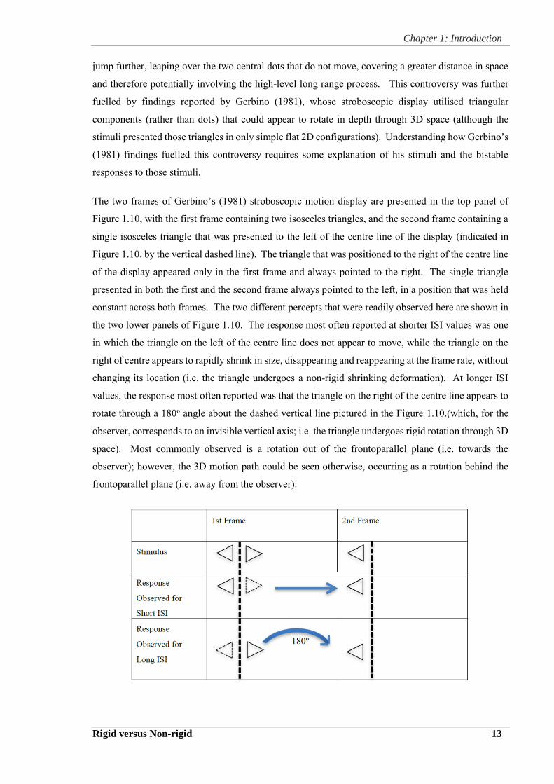
The two frames of Gerbino’s (1981) stroboscopic motion display are presented in the top panel of
Figure 1.10, with the first frame containing two isosceles triangles, and the second frame containing a
single isosceles triangle that was presented to the left of the centre line of the display (indicated in
Figure 1.10. by the vertical dashed line). The triangle that was positioned to the right of the centre line
of the display appeared only in the first frame and always pointed to the right. The single triangle
presented in both the first and the second frame always pointed to the left, in a position that was held
constant across both frames. The two different percepts that were readily observed here are shown in
the two lower panels of Figure 1.10. The response most often reported at shorter ISI values was one
in which the triangle on the left of the centre line does not appear to move, while the triangle on the
right of centre appears to rapidly shrink in size, disappearing and reappearing at the frame rate, without
changing its location (i.e. the triangle undergoes a non-rigid shrinking deformation). At longer ISI
values, the response most often reported was that the triangle on the right of the centre line appears to
rotate through a 180o angle about the dashed vertical line pictured in the Figure 1.10.(which, for the
observer, corresponds to an invisible vertical axis; i.e. the triangle undergoes rigid rotation through 3D
space). Most commonly observed is a rotation out of the frontoparallel plane (i.e. towards the
observer); however, the 3D motion path could be seen otherwise, occurring as a rotation behind the
frontoparallel plane (i.e. away from the observer).
Chapter 1: Introduction
Rigid versus Non-rigid 14
Figure 1.10. A pair of isosceles triangles appears in the 1st frame; the triangle on the right disappears when the
frames are viewed at short ISI. At a longer ISI the triangle on the right rotates out of the frontoparallel plane
through a 180o angle and terminates at the position of the triangle on the left (i.e. it lands on top of the triangle
on the left).
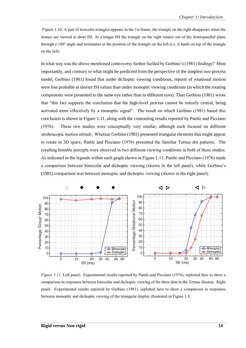
In what way was the above-mentioned controversy further fuelled by Gerbino’s (1981) findings? Most
importantly, and contrary to what might be predicted from the perspective of the simplest two-process
model, Gerbino (1981) found that under dichoptic viewing conditions, reports of rotational motion
were less probable at shorter ISI values than under monoptic viewing conditions (in which the rotating
components were presented to the same eye rather than to different eyes). Thus Gerbino (1981) wrote
that “this fact supports the conclusion that the high-level process cannot be entirely central, being
activated more effectively by a monoptic signal”. The result on which Gerbino (1981) based this
conclusion is shown in Figure 1.11, along with the contrasting results reported by Pantle and Picciano
(1976). These two studies were conceptually very similar, although each focused on different
stroboscopic motion stimuli. Whereas Gerbino (1981) presented triangular elements that might appear
to rotate in 3D space, Pantle and Picciano (1976) presented the familiar Ternus dot patterns. The
resulting bistable percepts were observed in two different viewing conditions in both of these studies.
As indicated in the legends within each graph shown in Figure 1.11, Pantle and Picciano (1976) made
a comparison between binocular and dichoptic viewing (shown in the left panel), while Gerbino’s
(1981) comparison was between monoptic and dichoptic viewing (shown in the right panel).
Figure 1.11. Left panel: Experimental results reported by Pantle and Picciano (1976), replotted here to show a
comparison in responses between binocular and dichoptic viewing of the three dots in the Ternus illusion. Right
panel: Experimental results reported by Gerbino (1981), replotted here to show a comparison in responses
between monoptic and dichoptic viewing of the triangular display illustrated in Figure 1.8.
Chapter 1: Introduction
Rigid versus Non-rigid 15
Just as described above for the Ternus display (see Figure 1.5.), Pantle and Picciano (1976) showed a
cyclic alternation between two stimulus frames, each of which contained three identical dots. The
horizontal row of the dots shown in Frame 1 was displayed at shifted position in Frame 2, such that
two of the dot positions overlapped with the previous ones. The influence of viewing condition on the
reported motion is shown above in the right panel of Figure 1.11.: The observer reported both group
and element motions in the binocular viewing, but the dichoptic viewing only resulted in the group
motion. Observers reported more element motion at the short ISI values (from 5ms to 30ms), whereas
more reports of group motion were obtained at the longer ISI values (from 30ms to 100ms). This
pattern of results was not obtained under similar conditions in Gerbino’s (1981) study. As can be
seen in the right panel of Figure 1.11, the growth in percentage of rotational motion reported under
two contrasted viewing conditions was not so different.
When the duration of ISI was between 5ms and 20ms, the added right triangle appeared to shrink in
place. When the duration of ISI became longer than 20ms, however, the triangle on the right appeared
to be rigidly rotating through 3D space (i.e. maintaining its shape, rather than deforming in its
position). If Gerbino’s (1981) findings followed closely the findings reported by Pantle and Picciano,
the dichoptic viewing in Gerbino’s study should have only given rise to rotation through space, but
not shrinking in place; this, however, was clearly not the case. The shrinking percept was taken by
Gerbino (1981) to imply a local identification process. The surprising result was that Gerbino’s (1981)
monoptic display gave rise to a greater proportion of rotation reports at short ISIs than did dichoptic
display.
To be clear, Gerbino’s (1981) findings support the hypothesised distinction between a low-level and a
high-level process, and also the notion of their sequential organisation. Consistent with the argument
presented by Pantle and Picciano (1976), Gerbino (1981) concluded that the high-level process could
generate the perception of rotation in the triangle display whenever the ISI was sufficiently long
(greater than about 30 ms). For Pantle and Picciano (1976), however, the low level process was
associated with a ‘local identity signal’ that was generated only in monoptic viewing and not in
dichoptic viewing. In contrast, Gerbino (1981) concluded that the high-level process could generate
the perception of rotation in the triangle display even in monoptic viewing, whenever the sequence of
stimuli represented the offset of the triangle on the right side and the subsequent onset of the triangle
on the left.
Gerbino’s (1981) specific contribution was effectively to question the stage at which the high-level
processing occurs. He also noted the significance of variations in the ISI. Such variations also
contradict the idea that there is a single threshold value of ISI at which the transition between the two
processes must occur (Barbur, 1980). The constraints imposed by the low-level process as described

Chapter 1: Introduction
Rigid versus Non-rigid 16
by (Pantle and Picciano, 1976) seem to be at odds with the observed variability in the dependence of
apparent motion on the temporal variable ISI.
Cavanagh and Mather (1989) argued that Braddick’s proposition about short-range and long-range
motion processes was based on exceptions. For instance, Braddick had claimed that the short-range
motion process could not react to equiluminant colour stimuli, but their study showed that there were
conditions under which equiluminant stimuli could actually lead to motion percepts in a short-range
process. Hence, Cavanagh and Mather (1989) recommended a separation of ‘first-order’ and ‘second-
order’ stimuli based on their measurements of the definition for the stimuli. Because their research
focus was on motion detection and analysis in general, they were unable to explain bistability of the
Ternus display and how a distinction between ‘first-order’ and ‘second-order’ stimuli contributes to
understanding how different percepts could be produced under different stimulus conditions.
Scott-Samuel and Hess (2001), however, disagreed with the view that element movement was
produced by a short-range process. In fact, they supported the argument that long-range process
produced both element and group movement in apparent movement. Despite these divergent opinions,
the two-processes model has been accepted as relevant to the perception of apparent motion (Gerbino,
1981; 1984).
1.4 Early Work on Apparent Motion
Studies of such apparent motion began more than 100 years ago. Even at that time, there was already
considerable interest in the role of cognitive factors in determining the characteristics of apparent
motion.
Exner (1888), for example, had shown that, when two lights flick on and off, the direction of the flashes
(i.e. left to right or vice versa,) cannot be perceived by looking at them. The observer can perceive the
change in position but only by perceiving the motion, so the observer perceives the motion directly
without perceiving the actual position at which the object starts or stops. So when the two lights are
shown in rapid succession with a delay in between, instead of seeing one of them move from one
position to the other, the observer sees the motion in one direction or another without knowing the
position or the end points.
Wertheimer (1912) extended this work and replaced sparks with vertical lines. The findings of his
study showed that, when the interval time between two spatially distanced vertical lines appearing one
after another was short, the two lines appeared to be on and off concurrently. If the interval time was
intermediate, a single line appeared to be moving from one position to the other, which means the
observers perceived the apparent motion, but if the interval time was longer (e.g. greater than one-
tenth of a second), one line appeared for some time and then the other line appeared for some time at

Chapter 1: Introduction
Rigid versus Non-rigid 17
the other location. Wertheimer also tried to determine whether the observed apparent motion occurred
at a retinal or central locus, so he developed a demonstration of interocular transfer in apparent motion
by separating views presented to the two eyes. Since cortical involvement was not well understood at
that time, he attributed the apparent motion to a short-circuiting of current flow in the brain. Today the
responses of direction-selective neurons provide a much better explanation (Sekuler and Blake, 2006),
but such investigation is beyond the scope of the current study.
A related issue is addressed in the present study, that being the problem of the how the visual system
detects the correspondence between the view of an object at one moment and a different view of the
same object seen at another moment. Wertheimer’s demonstration proves that detecting
correspondence over time is a precondition for motion perception and, in order to determine the
movement, the observer needs to decide whether the element in one frame matches or corresponds to
the element in the other (Sekuler and Blake, 2006). The Ternus Display has been used to study the
correspondence problem in motion perception.
Wertheimer’s (1921) pioneering work in this area also included investigations of how shifts in an
observer’s attention could change the appearance of apparent motion (see Sekuler, 2012, for a more
in-depth discussion of this facet of Wertheimer’s work). Although the study of apparent motion might
be unfamiliar to most people, virtually everyone has experienced apparent motion when watching a
movie or a television program. The mystery of the cinema is how a sequence of stationary movie
frames projected onto a large screen creates the appearance of motion, even though there is no real
motion. An exception occurs in those rare individuals who have a defect of motion perception due to
cerebral lesions, termed akinetopsia (see Rizzo, 1995). Wertheimer (Sekuler, 1996) was motivated to
determine whether failing to see the real motion also results in failing to see apparent motion. He
observed that the patient who has impaired motion perception could still recognise the colour of the
moving object.
Finally, some explanation of the standard practice in film projection should be inserted here. The
relation between the stroboscopic presentation of image sequences in film projection and the apparent
motion studied in the lab should be clear. However, the technology has been developed over many
years, and has reached a point at which the rapid display of static images has come to present what
looks like real motion. While the standard frame rate for movies is 24 frames per second (fps),
recently, a higher rate has been introduced into commercial film release (Cardinal, 2013). For example,
Peter Jackson’s film The Hobbit: An unexpected journey used 48 fps, along with stereoscopic
presentation (Cardinal, 2013). The advantage of 48 fps is that slow-motion scenes are smoother and
individual frames are sharper because faster sampling does not cause “strobing” (Cardinal, 2013). An
important detail of the projection is that blank images are inserted in between the actual image frames
in order to make the action appear smoother. Before the next image frame projects onto the screen, the
Chapter 1: Introduction
Rigid versus Non-rigid 18
previous image needs to be removed, but an intervening blank image must also be presented. Without
the gap in between the two successive images, the action looks unreal. At the faster frame rate, the
“strobing” or “flickering” does not occur.
1.4.1 The Motion After-effect (MAE)
Another interesting phenomenon in visual perception is the motion after-effect (MAE), which refers
to the powerful illusion of motion triggered by prior exposure to motion in the opposite direction
(Anstis et al., 1998). After prolonged viewing of stimuli moving continuously in one direction over a
period of time, the observer sees the same stimuli at rest appearing to move in the opposite direction
(Addams, 1834; Sekuler and Ganz, 1963; Pantle and Sekuler, 1968).
The initial discovery was made in the natural environment. For example, when an observer stares at a
waterfall flowing downwards for a period of time (e.g. 60 seconds) and then shifts gaze to a stationary
object like a nearby rock, the rock appears to be drifting upwards. In the second half of the 19th century,
investigation of the MAE was taken into the laboratory with the aid of Plateau’s spiral, which created
a spatio-temporal distortion of the visual field that lasted for some time after prolonged viewing (Wade,
1994). The duration of the MAE has always been used as a measurement of its strength. A substantial
body of research on space and motion perception in relation to MAE has identified a link between
psychophysics and physiology in the context of monocular and binocular channels in the visual
system. Although the phenomenon seems simple, research has revealed surprising complexities in the
postulated underlying mechanisms, although implying general principles regarding how the brain
processes visual information. In the last decade alone, more than 200 papers have been published that
deal with a MAE, largely inspired by improved techniques for examining brain electrophysiology and
by emerging theories of motion perception (Mather, Verstraten and Anstis, 1998). For example, Anstis
and Moulden (1970) found from their experimental results that the MAE contains both peripheral and
central components (a more detailed discussion of this MAE study is presented in Chapter 2).
It was found that, if the observer’s attention is engaged in a demanding distractor task rather than
concentrating on the adapting motion, the duration of a MAE will be greatly reduced (Chaudhuri,
1990). Attention is regarded as a process of selection in which cognitive resources are allocated to a
certain spatial location or object and the early-selection model supports the view that rudimentary
visual processing occurs automatically or ‘pre-attentively’ (Alais, 2005). Attentional selection to an
element of the pre-attentive map is needed to realise a complete percept of that element (Moray, 1959;
Neiseer and Becklen, 1975). Näätänen (1990 &1992) and Alms (2005) suggested that the encoding of
basic attributes such as motion was neither prior to the realm of attention nor automatic, so even a
salient motion stimulus should require some amount of directed attention.
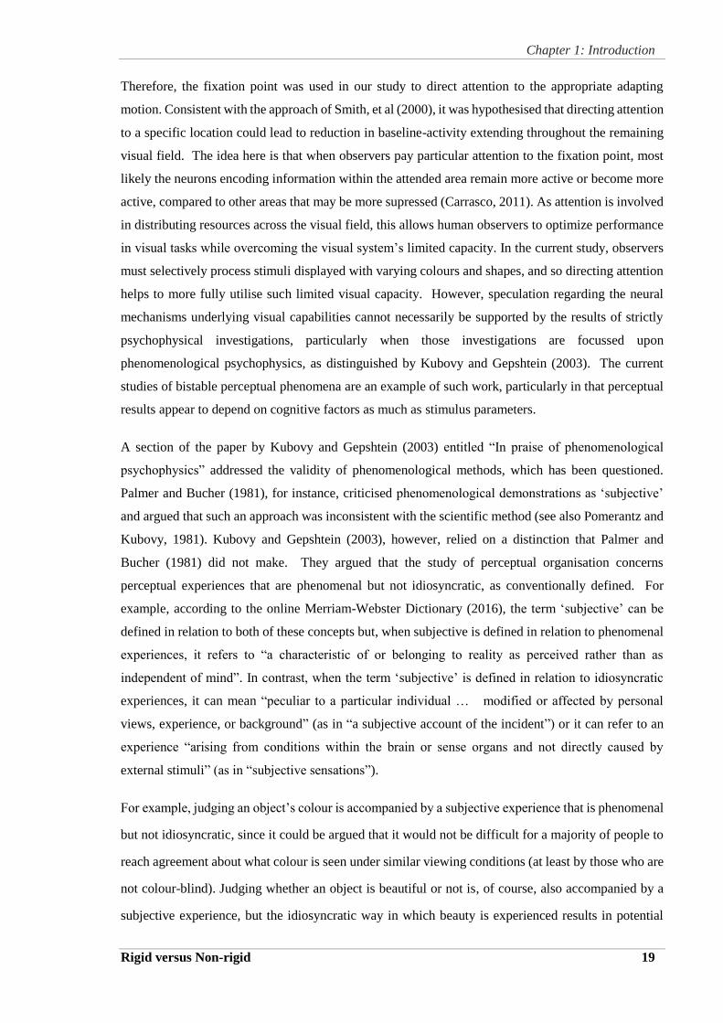
Chapter 1: Introduction
Rigid versus Non-rigid 19
Therefore, the fixation point was used in our study to direct attention to the appropriate adapting
motion. Consistent with the approach of Smith, et al (2000), it was hypothesised that directing attention
to a specific location could lead to reduction in baseline-activity extending throughout the remaining
visual field. The idea here is that when observers pay particular attention to the fixation point, most
likely the neurons encoding information within the attended area remain more active or become more
active, compared to other areas that may be more supressed (Carrasco, 2011). As attention is involved
in distributing resources across the visual field, this allows human observers to optimize performance
in visual tasks while overcoming the visual system’s limited capacity. In the current study, observers
must selectively process stimuli displayed with varying colours and shapes, and so directing attention
helps to more fully utilise such limited visual capacity. However, speculation regarding the neural
mechanisms underlying visual capabilities cannot necessarily be supported by the results of strictly
psychophysical investigations, particularly when those investigations are focussed upon
phenomenological psychophysics, as distinguished by Kubovy and Gepshtein (2003). The current
studies of bistable perceptual phenomena are an example of such work, particularly in that perceptual
results appear to depend on cognitive factors as much as stimulus parameters.
A section of the paper by Kubovy and Gepshtein (2003) entitled “In praise of phenomenological
psychophysics” addressed the validity of phenomenological methods, which has been questioned.
Palmer and Bucher (1981), for instance, criticised phenomenological demonstrations as ‘subjective’
and argued that such an approach was inconsistent with the scientific method (see also Pomerantz and
Kubovy, 1981). Kubovy and Gepshtein (2003), however, relied on a distinction that Palmer and
Bucher (1981) did not make. They argued that the study of perceptual organisation concerns
perceptual experiences that are phenomenal but not idiosyncratic, as conventionally defined. For
example, according to the online Merriam-Webster Dictionary (2016), the term ‘subjective’ can be
defined in relation to both of these concepts but, when subjective is defined in relation to phenomenal
experiences, it refers to “a characteristic of or belonging to reality as perceived rather than as
independent of mind”. In contrast, when the term ‘subjective’ is defined in relation to idiosyncratic
experiences, it can mean “peculiar to a particular individual … modified or affected by personal
views, experience, or background” (as in “a subjective account of the incident”) or it can refer to an
experience “arising from conditions within the brain or sense organs and not directly caused by
external stimuli” (as in “subjective sensations”).
For example, judging an object’s colour is accompanied by a subjective experience that is phenomenal
but not idiosyncratic, since it could be argued that it would not be difficult for a majority of people to
reach agreement about what colour is seen under similar viewing conditions (at least by those who are
not colour-blind). Judging whether an object is beautiful or not is, of course, also accompanied by a
subjective experience, but the idiosyncratic way in which beauty is experienced results in potential
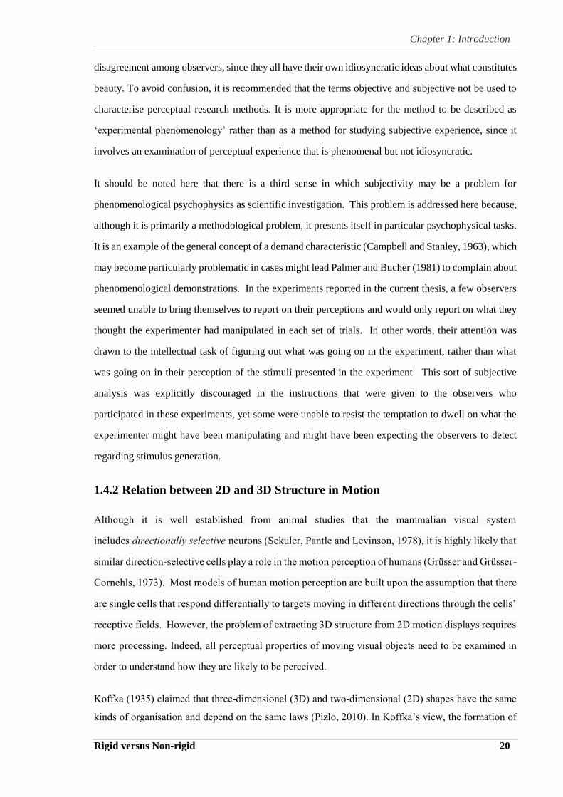
Chapter 1: Introduction
Rigid versus Non-rigid 20
disagreement among observers, since they all have their own idiosyncratic ideas about what constitutes
beauty. To avoid confusion, it is recommended that the terms objective and subjective not be used to
characterise perceptual research methods. It is more appropriate for the method to be described as
‘experimental phenomenology’ rather than as a method for studying subjective experience, since it
involves an examination of perceptual experience that is phenomenal but not idiosyncratic.
It should be noted here that there is a third sense in which subjectivity may be a problem for
phenomenological psychophysics as scientific investigation. This problem is addressed here because,
although it is primarily a methodological problem, it presents itself in particular psychophysical tasks.
It is an example of the general concept of a demand characteristic (Campbell and Stanley, 1963), which
may become particularly problematic in cases might lead Palmer and Bucher (1981) to complain about
phenomenological demonstrations. In the experiments reported in the current thesis, a few observers
seemed unable to bring themselves to report on their perceptions and would only report on what they
thought the experimenter had manipulated in each set of trials. In other words, their attention was
drawn to the intellectual task of figuring out what was going on in the experiment, rather than what
was going on in their perception of the stimuli presented in the experiment. This sort of subjective
analysis was explicitly discouraged in the instructions that were given to the observers who
participated in these experiments, yet some were unable to resist the temptation to dwell on what the
experimenter might have been manipulating and might have been expecting the observers to detect
regarding stimulus generation.
1.4.2 Relation between 2D and 3D Structure in Motion
Although it is well established from animal studies that the mammalian visual system
includes directionally selective neurons (Sekuler, Pantle and Levinson, 1978), it is highly likely that
similar direction-selective cells play a role in the motion perception of humans (Grüsser and Grüsser-
Cornehls, 1973). Most models of human motion perception are built upon the assumption that there
are single cells that respond differentially to targets moving in different directions through the cells’
receptive fields. However, the problem of extracting 3D structure from 2D motion displays requires
more processing. Indeed, all perceptual properties of moving visual objects need to be examined in
order to understand how they are likely to be perceived.
Koffka (1935) claimed that three-dimensional (3D) and two-dimensional (2D) shapes have the same
kinds of organisation and depend on the same laws (Pizlo, 2010). In Koffka’s view, the formation of
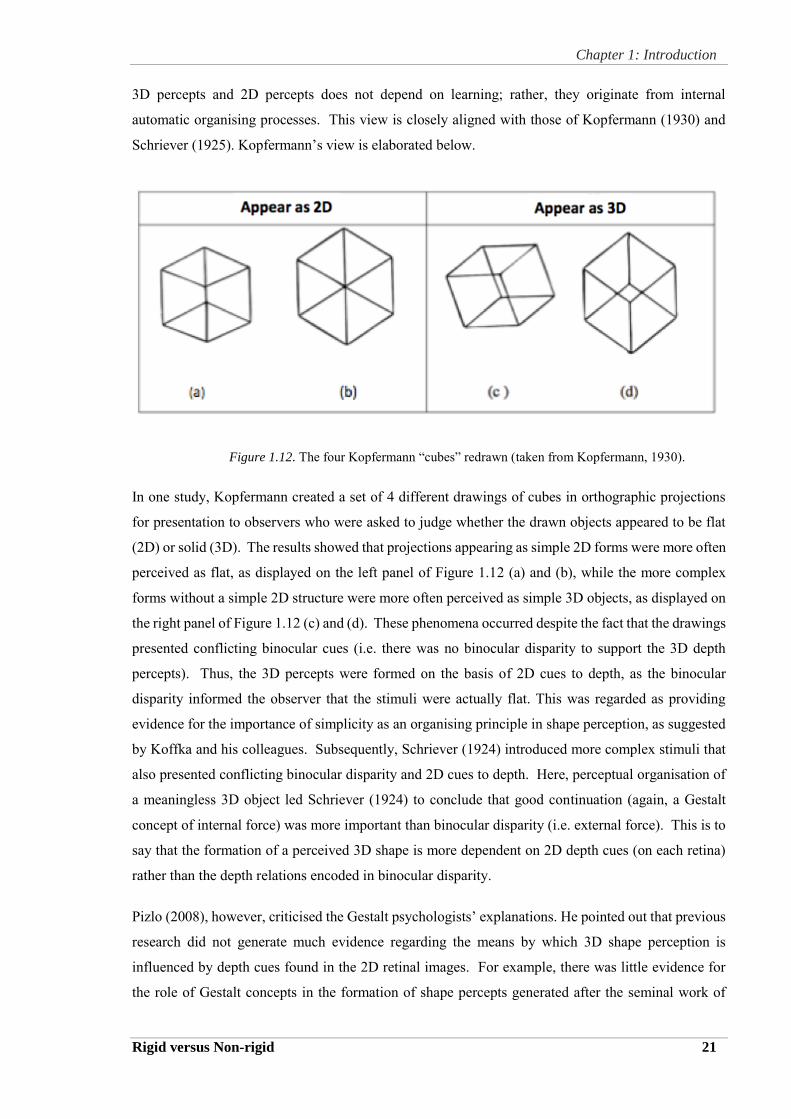
Chapter 1: Introduction
Rigid versus Non-rigid 21
3D percepts and 2D percepts does not depend on learning; rather, they originate from internal
automatic organising processes. This view is closely aligned with those of Kopfermann (1930) and
Schriever (1925). Kopfermann’s view is elaborated below.
Figure 1.12. The four Kopfermann “cubes” redrawn (taken from Kopfermann, 1930).
In one study, Kopfermann created a set of 4 different drawings of cubes in orthographic projections
for presentation to observers who were asked to judge whether the drawn objects appeared to be flat
(2D) or solid (3D). The results showed that projections appearing as simple 2D forms were more often
perceived as flat, as displayed on the left panel of Figure 1.12 (a) and (b), while the more complex
forms without a simple 2D structure were more often perceived as simple 3D objects, as displayed on
the right panel of Figure 1.12 (c) and (d). These phenomena occurred despite the fact that the drawings
presented conflicting binocular cues (i.e. there was no binocular disparity to support the 3D depth
percepts). Thus, the 3D percepts were formed on the basis of 2D cues to depth, as the binocular
disparity informed the observer that the stimuli were actually flat. This was regarded as providing
evidence for the importance of simplicity as an organising principle in shape perception, as suggested
by Koffka and his colleagues. Subsequently, Schriever (1924) introduced more complex stimuli that
also presented conflicting binocular disparity and 2D cues to depth. Here, perceptual organisation of
a meaningless 3D object led Schriever (1924) to conclude that good continuation (again, a Gestalt
concept of internal force) was more important than binocular disparity (i.e. external force). This is to
say that the formation of a perceived 3D shape is more dependent on 2D depth cues (on each retina)
rather than the depth relations encoded in binocular disparity.
Pizlo (2008), however, criticised the Gestalt psychologists’ explanations. He pointed out that previous
research did not generate much evidence regarding the means by which 3D shape perception is
influenced by depth cues found in the 2D retinal images. For example, there was little evidence for
the role of Gestalt concepts in the formation of shape percepts generated after the seminal work of
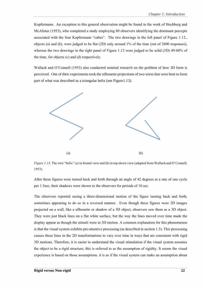
Chapter 1: Introduction
Rigid versus Non-rigid 22
Kopfermann. An exception to this general observation might be found in the work of Hochberg and
McAlister (1953), who completed a study employing 80 observers identifying the dominant percepts
associated with the four Kopfermann “cubes”. The two drawings in the left panel of Figure 1.12.,
objects (a) and (b), were judged to be flat (2D) only around 1% of the time (out of 2600 responses),
whereas the two drawings in the right panel of Figure 1.12 were judged to be solid (3D) 49-60% of
the time, for objects (c) and (d) respectively.
Wallach and O’Connell (1953) also conducted seminal research on the problem of how 3D form is
perceived. One of their experiments took the silhouette projections of two wires that were bent to form
part of what was described as a triangular helix (see Figure1.13).
(a) (b)
Figure 1.13. The wire “helix” (a) in frontal view and (b) in top-down view (adapted from Wallach and O’Connell,
1953).
After these figures were turned back and forth through an angle of 42 degrees at a rate of one cycle
per 1.5sec, their shadows were shown to the observers for periods of 10 sec.
The observers reported seeing a three-dimensional motion of the figure turning back and forth,
sometimes appearing to do so in a reversed manner. Even though these figures were 2D images
projected on a wall, like a silhouette or shadow of a 3D object, observers saw them as a 3D object.
They were just black lines on a flat white surface, but the way the lines moved over time made the
display appear as though the stimuli were in 3D motion. A common explanation for this phenomenon
is that the visual system exhibits pre-attentive processing (as described in section 1.3). This processing
causes these lines in the 2D transformations to vary over time in ways that are consistent with rigid
3D motions. Therefore, it is easier to understand the visual stimulation if the visual system assumes
the object to be a rigid structure; this is referred to as the assumption of rigidity. It seems the visual
experience is based on those assumptions. it is as if the visual system can make an assumption about
Chapter 1: Introduction
Rigid versus Non-rigid 23
what it observes in the world, and then tests its hypothesis about what exists in the world against direct
sensory experience.
Of course, it may be that studies using stimuli with only two dimensions are insufficient to uncover
how simplicity constraints can make up for information lost in the projection from 3D objects to 2D
stimuli. In addition to binocular parallax, another source of depth cues that could be introduced into
the stimuli would be motion parallax (an arguably stronger cue to depth than binocular parallax). A
great deal of work has been done with such stimuli, but the most relevant to the current discussion is
that of Shepard and Metzler (1971).
Shepard and Metzler (1971) conducted experiments which found that the time required to decide
whether two perspective views depict the same three dimensional object is a linear function of the
angular difference between the two orientations portrayed. Based on this finding, they further explored
the possible role of perceptual mechanisms in mental rotation by presenting two perspective views of
a three dimensional object that appeared to be rotating back and forth in the two dimensional picture
plane. Apparently their 2D stimuli proved that the 2D image could produce a 3D percept of shape that
is not influenced by any viewing orientation either from the picture plane or in depth. According to
Shepard and Metzler (1971), observers made the comparison by processing a mental analog of the
actual physical rotation of one object into resemblance with the other, as the internal process is a mental
analogy of an external process. Similarly, the internal process is important to the perceptual process
that would be carried out if a subject watched the corresponding physical rotation. Therefore, it is
possible to consider that the internal travelling time is related to the time in the external physical
rotation. Accordingly, such three dimensional objects are very interesting shapes to use in
investigating perception.
To be precise, the rectangular boxes comprising the stimuli presented in the current experiments must
be identified as ‘right’ prisms (Weisstein, 2016) in order to clearly distinguish them from solid objects
formed by connecting polygons for which the joining edges and faces are not perpendicular to each
other (in which case the objects would be identified as ‘oblique’ prisms) (Weisstein, 2016). Hence,
when ‘the rectangular’ is used in this thesis, it refers to the 2D shape. When ‘the rectangular box’ is
used, it refers to the 3D right prism.
1.4.3 Recognition-by-Components and the Correspondence Problem
Later, Biederman (1987) developed his theory of shape reconstruction based on “recognition-by-
components” (RBC). Biederman reviewed all the important milestones in the history of shape
perception, identifying errors and reaction times observed during both recognition and reconstruction
experiments on 3D shape. He tested his theory via computer simulations and in psychophysical
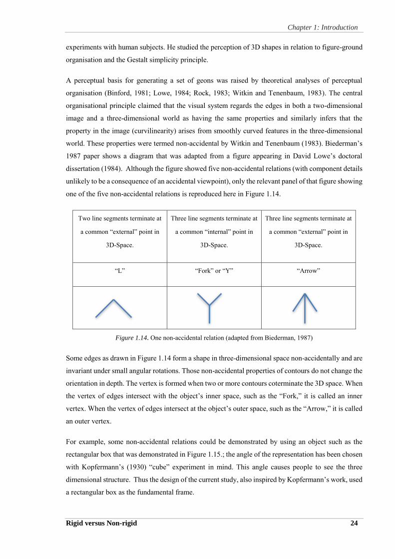
Chapter 1: Introduction
Rigid versus Non-rigid 24
experiments with human subjects. He studied the perception of 3D shapes in relation to figure-ground
organisation and the Gestalt simplicity principle.
A perceptual basis for generating a set of geons was raised by theoretical analyses of perceptual
organisation (Binford, 1981; Lowe, 1984; Rock, 1983; Witkin and Tenenbaum, 1983). The central
organisational principle claimed that the visual system regards the edges in both a two-dimensional
image and a three-dimensional world as having the same properties and similarly infers that the
property in the image (curvilinearity) arises from smoothly curved features in the three-dimensional
world. These properties were termed non-accidental by Witkin and Tenenbaum (1983). Biederman’s
1987 paper shows a diagram that was adapted from a figure appearing in David Lowe’s doctoral
dissertation (1984). Although the figure showed five non-accidental relations (with component details
unlikely to be a consequence of an accidental viewpoint), only the relevant panel of that figure showing
one of the five non-accidental relations is reproduced here in Figure 1.14.
Two line segments terminate at
a common “external” point in
3D-Space.
Three line segments terminate at
a common “internal” point in
3D-Space.
Three line segments terminate at
a common “external” point in
3D-Space.
“L” “Fork” or “Y” “Arrow”
Figure 1.14. One non-accidental relation (adapted from Biederman, 1987)
Some edges as drawn in Figure 1.14 form a shape in three-dimensional space non-accidentally and are
invariant under small angular rotations. Those non-accidental properties of contours do not change the
orientation in depth. The vertex is formed when two or more contours coterminate the 3D space. When
the vertex of edges intersect with the object’s inner space, such as the “Fork,” it is called an inner
vertex. When the vertex of edges intersect at the object’s outer space, such as the “Arrow,” it is called
an outer vertex.
For example, some non-accidental relations could be demonstrated by using an object such as the
rectangular box that was demonstrated in Figure 1.15.; the angle of the representation has been chosen
with Kopfermann’s (1930) “cube” experiment in mind. This angle causes people to see the three
dimensional structure. Thus the design of the current study, also inspired by Kopfermann’s work, used
a rectangular box as the fundamental frame.
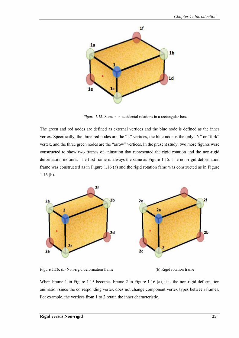
Chapter 1: Introduction
Rigid versus Non-rigid 25
Figure 1.15. Some non-accidental relations in a rectangular box.
The green and red nodes are defined as external vertices and the blue node is defined as the inner
vertex. Specifically, the three red nodes are the “L” vertices, the blue node is the only “Y” or “fork”
vertex, and the three green nodes are the “arrow” vertices. In the present study, two more figures were
constructed to show two frames of animation that represented the rigid rotation and the non-rigid
deformation motions. The first frame is always the same as Figure 1.15. The non-rigid deformation
frame was constructed as in Figure 1.16 (a) and the rigid rotation fame was constructed as in Figure
1.16 (b).
Figure 1.16. (a) Non-rigid deformation frame (b) Rigid rotation frame
When Frame 1 in Figure 1.15 becomes Frame 2 in Figure 1.16 (a), it is the non-rigid deformation
animation since the corresponding vertex does not change component vertex types between frames.
For example, the vertices from 1 to 2 retain the inner characteristic.
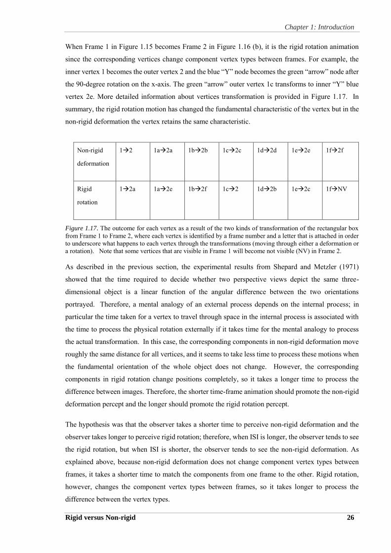
Chapter 1: Introduction
Rigid versus Non-rigid 26
When Frame 1 in Figure 1.15 becomes Frame 2 in Figure 1.16 (b), it is the rigid rotation animation
since the corresponding vertices change component vertex types between frames. For example, the
inner vertex 1 becomes the outer vertex 2 and the blue “Y” node becomes the green “arrow” node after
the 90-degree rotation on the x-axis. The green “arrow” outer vertex 1c transforms to inner “Y” blue
vertex 2e. More detailed information about vertices transformation is provided in Figure 1.17. In
summary, the rigid rotation motion has changed the fundamental characteristic of the vertex but in the
non-rigid deformation the vertex retains the same characteristic.
Non-rigid
deformation
12 1a2a 1b2b 1c2c 1d2d 1e2e 1f2f
Rigid
rotation
12a 1a2e 1b2f 1c2 1d2b 1e2c 1fNV
Figure 1.17. The outcome for each vertex as a result of the two kinds of transformation of the rectangular box
from Frame 1 to Frame 2, where each vertex is identified by a frame number and a letter that is attached in order
to underscore what happens to each vertex through the transformations (moving through either a deformation or
a rotation). Note that some vertices that are visible in Frame 1 will become not visible (NV) in Frame 2.
As described in the previous section, the experimental results from Shepard and Metzler (1971)
showed that the time required to decide whether two perspective views depict the same three-
dimensional object is a linear function of the angular difference between the two orientations
portrayed. Therefore, a mental analogy of an external process depends on the internal process; in
particular the time taken for a vertex to travel through space in the internal process is associated with
the time to process the physical rotation externally if it takes time for the mental analogy to process
the actual transformation. In this case, the corresponding components in non-rigid deformation move
roughly the same distance for all vertices, and it seems to take less time to process these motions when
the fundamental orientation of the whole object does not change. However, the corresponding
components in rigid rotation change positions completely, so it takes a longer time to process the
difference between images. Therefore, the shorter time-frame animation should promote the non-rigid
deformation percept and the longer should promote the rigid rotation percept.
The hypothesis was that the observer takes a shorter time to perceive non-rigid deformation and the
observer takes longer to perceive rigid rotation; therefore, when ISI is longer, the observer tends to see
the rigid rotation, but when ISI is shorter, the observer tends to see the non-rigid deformation. As
explained above, because non-rigid deformation does not change component vertex types between
frames, it takes a shorter time to match the components from one frame to the other. Rigid rotation,
however, changes the component vertex types between frames, so it takes longer to process the
difference between the vertex types.
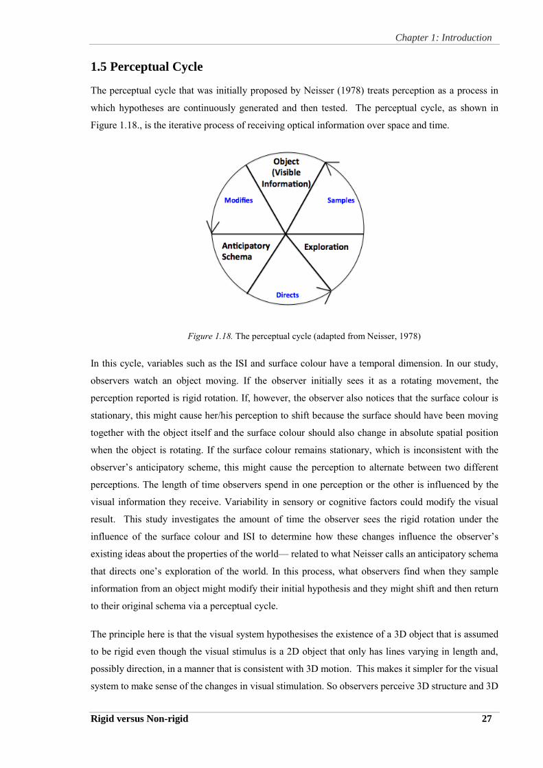
Chapter 1: Introduction
Rigid versus Non-rigid 27
1.5 Perceptual Cycle
The perceptual cycle that was initially proposed by Neisser (1978) treats perception as a process in
which hypotheses are continuously generated and then tested. The perceptual cycle, as shown in
Figure 1.18., is the iterative process of receiving optical information over space and time.
Figure 1.18. The perceptual cycle (adapted from Neisser, 1978)
In this cycle, variables such as the ISI and surface colour have a temporal dimension. In our study,
observers watch an object moving. If the observer initially sees it as a rotating movement, the
perception reported is rigid rotation. If, however, the observer also notices that the surface colour is
stationary, this might cause her/his perception to shift because the surface should have been moving
together with the object itself and the surface colour should also change in absolute spatial position
when the object is rotating. If the surface colour remains stationary, which is inconsistent with the
observer’s anticipatory scheme, this might cause the perception to alternate between two different
perceptions. The length of time observers spend in one perception or the other is influenced by the
visual information they receive. Variability in sensory or cognitive factors could modify the visual
result. This study investigates the amount of time the observer sees the rigid rotation under the
influence of the surface colour and ISI to determine how these changes influence the observer’s
existing ideas about the properties of the world— related to what Neisser calls an anticipatory schema
that directs one’s exploration of the world. In this process, what observers find when they sample
information from an object might modify their initial hypothesis and they might shift and then return
to their original schema via a perceptual cycle.
The principle here is that the visual system hypothesises the existence of a 3D object that is assumed
to be rigid even though the visual stimulus is a 2D object that only has lines varying in length and,
possibly direction, in a manner that is consistent with 3D motion. This makes it simpler for the visual
system to make sense of the changes in visual stimulation. So observers perceive 3D structure and 3D
Chapter 1: Introduction
Rigid versus Non-rigid 28
motion, even though it is simply the assumption of rigidity that produces this result. Without this
assumption underlying the perceptual hypotheses being tested, there would be competition between
these percepts and percepts of non-rigid transformation of those same structures. Gestalt Psychologists
also think that it is the simplicity of form that determines what likely will be perceived and, in some
ways, it is simpler for the visual system to assume the existence of a rigid object undergoing the 3D
transformations, rather than a 2D visual stimulus undergoing unusual 2D transformations. The
hypothesis of a rigid 3D structure is posed as an assumption by the visual system, which then proceeds
to form percepts by testing the direct sensory experience against the expected variations. The visual
system finds what observers already anticipated seeing if the sensory information is consistent with
the hypothesised existence of an object of rigid 3D structure simply rotating, and so the visual system
delivers this personal experience of a 3D object in motion. The percept is consistent with the
hypothesis, which is not rejected, and therefore accepted, even though other assumptions could have
been made. One such different assumption could be that the lines drawn in 2D on a flat card are getting
shorter or longer, and therefore twisting around in interesting ways that are hard to explain. These
displays could be presenting simple 2D motion on a 2D plane, so why does the visual system not allow
the stimuli to be perceived as such (i.e. 2D motion)? Yet such straightforward percepts are not often
perceived in these cases; rather, observers experience a sensory impression that is interpreted as 3D
motion.
So what will happen when observers are presented with two still images in rapid succession, each
showing the sort of rectangular boxes that are illustrated in the previous Figure 1.16.? The question is
whether the object will be seen as undergoing rigid rotation or non-rigid deformation. Non-rigid
deformation was seen to be less likely on the basis of the rigidity assumption. The rigidity assumption
does not work as well for stereo kinetic effects, yet when the ISI is in the proper range, the non-rigid
deformation is what the visual system delivers to observers, so there is an ambiguity from the stimulus.
Under those circumstances, therefore, more than one principle applies, and it seems that the common
explanation should be accepted—that when the visual system is given more time to process a line
drawing, it is more likely to “unconsciously assume” that 3D structure exists, and therefore, when
parsimonious, it will produce a 3D object rigidly rotating in the space rather than produce a 2D object
that is just deforming. Alternatively, the 3D deformation of the 3D object breaks the rigidity
assumption, as mentioned previously. In this case, the visual system seems to match the spatially
offset corresponding features between the stimuli across time frames. This seems to occur when
observers have insufficient time to recognise the whole structure. In contrast, when there is a short-
distance shift in the local structure (referring to the local corresponding details like the edges and
corners that are close to each other across the two frames of stroboscopic motion display), the more
likely perceptual result is the deformation of the 3D object presented with a relatively short ISI.
Chapter 1: Introduction
Rigid versus Non-rigid 29
There are a variety of proposed mechanisms (or models) that might be thought to underlie the
perception of rotation vs. deformation, including the feature matching that was introduced in the
previous section. There are more recent popular alternatives, such as the Bayesian framework
proposed by Weiss and Adelson (1998). They proposed that the visual system needs to combine
multiple local measurements to estimate the motion of an object as each of them carries separately
some degree of ambiguity. Hence, their study presented a model of motion perception whereby
measurements from different image regions are combined according to a Bayesian estimator (Weiss
and Adelson, 1998). In addition to this, and also the “Perceptual Cycle” introduced and discussed
above, there is a call to consider low-level neural models describing bi-stable perception, such as that
of Lang and Chow (2002), Noest and et al, (2007), or Moreno-Bote, Rinzel & Rubin (2007). Lang and
Chow presented a biologically plausible model of binocular rivalry consisting of a network of
Hodgkin-Huxley type neurons and explained the experimentally and psychophysically observed
phenomena. Noest and et al, (2007) presented a simple neural model that explains the observed
behavior and predicts several more complicated percept sequences, without invoking any “high-level”
decision making or memory. Moreno-Bote, Rinzel & Rubin (2007) made attempt to explain what
causes the bistable perceptual switches. They claimed that most existing models assume that switches
arise from a slow fatiguing process, such as adaptation or synaptic depression, so they developed a
new, attractor-based framework in which alternations are induced by noise and are absent without it.
Their model constructed a neutrally plausible attractor model goes beyond previous energy-based
conceptualizations of perceptual bistability and implemented in both firing rate mean-field and spiking
cell-based networks. The model accounts for known properties of bistable perceptual phenomena, most
notably the increase in alternation rate with stimulation strength observed in binocular rivalry. It also
makes a novel prediction about the effect of changing stimulus strength on the activity levels of the
dominant and suppressed neural populations. Although a comprehensive review of the literature on
such neural models is not attempted in this thesis, readers may well imagine how hypotheses could be
formed regarding perception based upon assumptions that are commonly made regarding underlying
neural models,such as those presented above.
1.5.1 Hypothesis
Inspired by others’ work, we selected a solid rectangular object for use in our study. Size and colour
were selected as the two dominant stimulus factors. Two sizes of the rectangular box, called fat sponge
and thin sponge, were used, and two surface colours were implemented with them as shown in Figure
1.19. In stroboscopic display, the fat rectangular box tended to be perceived as deforming, and the thin
rectangular box tended to be perceived as rotating.

Chapter 1: Introduction
Rigid versus Non-rigid 30
An object could be all-yellow (for example in Figure 1.19.); this is labelled monochrome, meaning
that all of the surface colours were yellow. Alternatively, another colour, green, could be used on one
of the surfaces (for example, the rectangular boxes shown in Figure 1.20.).
(a) (b)
Figure 1.19. (a) Fat sponge. (b) Thin sponge.
Figure 1.20. Rectangular box with green surface
Figure 1.21. Green-shifting to the side in a manner consistent with object rotation for both fat and thin
sponges when compared to Figure 1.20.
Therefore, there were three levels related to the surface colour of the sponge as below:
Green-stationary - a single green side always faces upwards (Figure 1.20)
Green-shifting - a single green side shifts in a manner consistent with rotation (Figure 1.21)
Monochrome - all visible sides are yellow (Figure 1.19.)
The following questions were generated:
Chapter 1: Introduction
Rigid versus Non-rigid 31
1. Is there an effect of changing surface colour on the perceived motion of a stroboscopically
displayed object?
2. When the changing surface colour is consistent with rigid rotation, does this make a report of rigid
rotation more likely?
3. When the changing surface colour is inconsistent with rigid rotation, does this make a report of
rigid rotation less likely?
What is fascinating about these last two questions is that one might be answered in the affirmative
while the other is answered in the negative. A plausible hypothesis is that the strongest effects on
perception will occur only when surface colour contradicts the motion that was otherwise more likely
to be seen under given conditions. Then the results might show such asymmetry in the influence of
changing surface colour: The answer could be “no” to question 2 while the answer could be “yes’ to
question 3.
The stimuli presented in the current study were designed via the factorial combination of two shapes
and three surface colours. An additional condition in which there was no surface colour manipulation
provided for a baseline result to be established as a control condition. Both of the stimulus shapes
(thin and fat sponges) were presented in this control condition, which can be thought of as the
monochrome (all yellow) condition, since no surface colour variation was imposed upon these stimuli
as it was in the experimental conditions. What was observed in all conditions was the shift in observers’
reports of perceiving non-rigid deformation versus rigid rotation for stroboscopically presented visual
stimuli appearing as sponges that exhibited one of these two types of motion. The baseline result
observed in the control condition showed the proportion of rigid rotation responses increasing as a
function of ISI, with a transition point between the two response alternatives when there was no
influence of changing surface colour, since there was only one colour (yellow) for all the visible
surfaces in the monochrome condition.
The hypothesis that was proposed here was that the greatest effects would be observed when surface
colour contradicted the motion that the observer was otherwise most likely to see. When the surface
colour did not contradict the motion the observers were already seeing, there would be no strong shift
in perception. This is a slightly cognitive interpretation, in which the observer’s understanding
demands consistency with the conventional rules followed by three dimensional objects. The retina,
of course, does not “know” rules about the surface colour, so the observers must first think about what
they see before they decide what they know about the stimulus. In this context, a two-stage process
may be proposed. In the first stage (the automatic periphery process), the ISI is the dominant influence
on the perception. In the second stage of processing, observers’ understanding of the object, including
the shape and surface colour, could influence what they report. This perspective could also lead to the
supposition that fatter objects “like to” deform and thinner objects “like to” rotate.
Chapter 1: Introduction
Rigid versus Non-rigid 32
processing provides the answer. In the first stage (the automatic periphery process), the ISI is the
dominant influence on the perception. In the second stage of processing, observers’ understanding of
the object, including the shape and surface colour, could influence what they report, which seems to
indicate that fatter objects like to deform and thinner objects like to rotate.
There could be some evidence here for pre-attentive processing, were there to be a strong influence on
perception of the temporal variable, ISI. The idea here is that, when details are consistent, there is no
need for a response to change because no extra thought is required. If an observer’s experience is
consistent with a perceptual hypothesis, then that hypothesis is simply retained; however, if a
hypothesis is contradicted by experience, then the perceptual response will need to change, as a new
hypothesis must be testsed. If indeed, the best model to describe this process is such a “perceptual
cycle,” as (Neisser, 1978) proposed, the bistable motion perception studied here may be thought of a
resulting from continuous updating of hypotheses by testing them against experience.
Conflicting cues will make observers change what they report, whereas consistent cues do not
necessarily affect what they report. Therefore when observers look at the proportion of the rigid
rotation as a function of ISI, having a surface colour that is either shifting or stationary as the way it is
consistent with what they already experiencing from the influence of shape. the fat object is generally
more likely to be seen as deforming, both the monochrome and green-stationary conditions do not
need the visual system to make the change. Only the green-shifting condition, which implies rigid
rotation motion, forces the visual interpretation to change. Therefore, reports should be affected most
strongly in the green-shifting condition for the fat sponges, where the proportion of rigid rotation
should be increase compared to the control condition; likewise, reports should be affected less in the
green-shifting condition for the thin sponge stimuli, since no contradictory input would be active to
modify the response proportions in comparison to the control condition.
So, in the case of thin object that the visual system seems to be preferred to be perceived as rotating,
both monochrome and green-shifting conditions have the same influence on the reported motion, since
rotation is consistent with the preferred interpretation of the object. Hence, there is no need for the
visual system to make the change for the thin sponge because the influence of surface colour has the
same effect as the influence of the shape. Only the green-stationary condition, which implies non-
rigid deformation motion, forces it to make the change.
Therefore when observers look at the proportion of the rigid rotation as a function of ISI, having a
surface colour that is either shifting or stationary as the way it is consistent with what they already
Chapter 1: Introduction
Rigid versus Non-rigid 33
experiencing from the influence of shape. If the influences from the shape and the surface colour are
consistent with each other, the visual system will not make the change; therefore, in the case of the fat
object that was suggested by the visual system to prefer deforming, both the monochrome and green-
stationary conditions do not need the visual system to make the change. Only the green-shifting
condition, which implies rigid rotation motion, forces the visual interpretation to change. Therefore,
reports should be affected the most in the green-shifting condition for the fat sponges, where the
proportion of rigid rotation should be increased compared to the control condition; however, reports
should be affected less in the green-shifting condition for the thin sponges since no contradictory
influence was then active to make any difference in response proportions in comparison to the control
condition.
The whole curve of the plotted proportion of rigid rotation responses would be expected to shifts up
or down based on the surface colour in these conditions. The hypothesis is consistent with Nessier’s
perceptual cycle (1978) as follows: The observer generates a perceptual hypothesis about what is out
there in the world; one hypothesis holding that an object is rotating, another hypothesis holding that
an object deforming. Observers generate these hypothesises and test them against their perceptual
experience, during which process sensory or cognitive factors operate to influence whether initial
hypotheses are retained or rejected.
1.6 Current Understanding of the Topic
Weilnhammer (2014) was motivated to study the endogenous nature of perceptual transitions and the
relation between sensory stimulation and conscious perception. As in our study, participants were
asked to report what they saw, rather than what they thought or analysed. Three parameters of the
Lissajous figure—complexity, line width and rotational speed—were the critical stimulus
configuration for the perceptual transitions of similar bistable depth-from-motion stimuli and they are
relevant to the timing and duration of depth-symmetrical self-occlusions of the figure (Pastukhov et
al., 2012; Stonkute et al., 2012). Accordingly, these parameters were manipulated to modify the
perceptual dominance durations and transition probabilities. In their experiment, one participant was
excluded because no perceptual transitions were reported in 4 out of 8 experimental conditions. Most
likely this particular participant did not simply report what was seen, but the purpose of the
experiments was to investigate the effects of the sensory stimulation rather than the observer’s
cognitive thinking or analysis. Our study also had to exclude two observers, as they were unable to
report any perceptual transitions. Their results showed that no participants reported any mixed or
unclear percepts by pressing the relevant button to report their percepts (Weilnhammer et al, 2014).
Self-occlusion occurred as often for the high-complexity as for the low-complexity figure, and the
dominance duration was longer for the low-complexity figure and shorter for the high-complexity
Lissajous stimulus, although the transition probabilities at critical positions of the stimulus were
Chapter 1: Introduction
Rigid versus Non-rigid 34
similar across both high-complexity and low-complexity. The factor “rotational speed” can overrule
the effect of complexity for the perceptual transitions since, when the rotational speed was faster, the
dominance durations were longer and the transition probabilities were lower. Therefore, the results
suggested different mechanisms could be applied to the effects of “complexity” and “rotational speed”,
respectively. By increasing the line width and decreasing the rotational speed, both these factors
significantly influenced perceptual transitions, and longer self-occlusion caused dominance durations.
The conclusion therefore was that prolonged self-occlusions for slowly rotating Lissajous stimuli was
not sufficient to explain the effect of rotational speed on perceptual dominance and the proposition
was that larger ‘momentum’ (Hubbard, 2005) can be caused by the higher rotational speed, which was
also related to lower transition rates.
Their study is somewhat analogous to the first experiment in our study. As shape is such a unique
characteristic for the object, it can be recognised from our conscious perception. Therefore the first
cognitive factor chosen for the first experiment was shape. The hypothesis tested in the first experiment
was that the shape can influence whether the rectangular box is undergoing non-rigid deformation or
rigid rotation. When the rectangular box is fatter, there should be more non-rigid deformation; when
the rectangular box is thinner, more rigid rotation should be reported. The basic sensory factor, ISI,
was also manipulated in the first experiment. It was proposed that both sensory and cognitive factors
would influence the perception. In addition, surface colour was manipulated in order to compete with
the ISI variation to see if this sensory factor would interact with the effects of shape and surface colour.
In other words, a central question here is the following: Will cognitive factors and sensory factors
integrate or compete with each other in determining which of two apparent motion percepts is
experienced? Further, if one factor is overridden by the other, will the addition of another similar
The aim of the first experiment to be reported here was to answer these questions for a particular set
of rectangular stimuli. The aim of the second experiment to be reported here was to compare
adaptation after-effects under a variety of conditions, but most particularly to contrast the effect of
what is presented during an adaptation period with what the adapting stimulus is ‘seen as’ during
adaptation, in contrast to an effect that depends upon variation in sensory stimulus parameter, even
when the observer is ‘unconscious’ of that variation.
Chapter 2: Literature Review
Rigid versus Non-rigid 35
CHAPTER 2: LITERATURE REVIEW
This chapter reviews the literature on key research areas related to our study, namely: multistable
apparent motion, perceptual organisation, and the motion after-effect (MAE), in addition to the more
specialised concepts to be introduced here, the association field and rigidity assumption. The chapter
also discusses in detail the investigation by Dodd, McAuley and Pratt (2005) that showed the
importance of the temporal variable, interstimulus interval (ISI). Particular attention is paid to
research by Ramachandran and Anstis (1985), which is similar to our second experiment in that it
used both unambiguous and ambiguous stimuli. Investigations of the Ternus Illusion conducted by
Petersik and Pantle (1979) and Petersik (1980), which emphasised the manipulation of ISI, are
discussed to explain why cycle duration was held constant in all of the experiments in the present
study. Next, studies related to the mechanisms underlying the two competing sensations are explored,
with particular focus on their operation as a peripheral or central process. Similar investigations into
whether the motion after-effect (MAE) is processed in central or peripheral components are also
reported. Finally, the association field is examined to explain rigid rotation and non-rigid deformation
and research associated with the rigidity assumption is discussed.
2.1 Multistable Apparent Motion
Exner (1888) pioneered the study of motion using intense electrical sparks from two sources (Sekuler
and Blake, 2006). Two sparks were placed apart, one on the left and the other on the right. The
observers were asked to judge which spark flashed first. It was observed that a longer time delay
between the two sparks made it easier for observers to make a judgement, but a shorter interval made
it more difficult. When Exner then reduced the distance between the two sparks, observers saw the
apparent motion of a spark travelling from one location to the other; they were asked to make a
judgement about which direction the spark travelled from. Finally, Exner placed two sparks next to
each other as a single bright spark and the observers could still see the apparent movement. The
finding that apparent motion cannot be resolved spatially has been confirmed in other research
(Thorson, Lang and Biederman-Thorson, 1969; Foster, Thorson, Mcllwin and Biederman-Thorson,
1981).
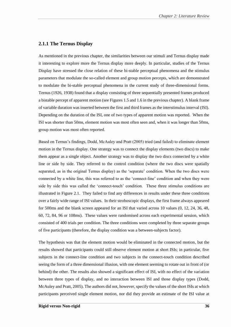
Chapter 2: Literature Review
Rigid versus Non-rigid 36
2.1.1 The Ternus Display
As mentioned in the previous chapter, the similarities between our stimuli and Ternus display made
it interesting to explore more the Ternus display more deeply. In particular, studies of the Ternus
Display have stressed the close relation of these bi-stable perceptual phenomena and the stimulus
parameters that modulate the so-called element and group motion percepts, which are demonstrated
to modulate the bi-stable perceptual phenomena in the current study of three-dimensional forms.
Ternus (1926, 1938) found that a display consisting of three sequentially presented frames produced
a bistable percept of apparent motion (see Figures 1.5 and 1.6 in the previous chapter). A blank frame
of variable duration was inserted between the first and third frames as the interstimulus interval (ISI).
Depending on the duration of the ISI, one of two types of apparent motion was reported. When the
ISI was shorter than 50ms, element motion was most often seen and, when it was longer than 50ms,
group motion was most often reported.
Based on Ternus’s findings, Dodd, McAuley and Pratt (2005) tried (and failed) to eliminate element
motion in the Ternus display. One strategy was to connect the display elements (two discs) to make
them appear as a single object. Another strategy was to display the two discs connected by a white
line or side by side. They referred to the control condition (where the two discs were spatially
separated, as in the original Ternus display) as the ‘separate’ condition. When the two discs were
connected by a white line, this was referred to as the ‘connect-line’ condition and when they were
side by side this was called the ‘connect-touch’ condition. These three stimulus conditions are
illustrated in Figure 2.1. They failed to find any differences in results under these three conditions
over a fairly wide range of ISI values. In their stroboscopic displays, the first frame always appeared
for 500ms and the blank screen appeared for an ISI that varied across 10 values (0, 12, 24, 36, 48,
60, 72, 84, 96 or 108ms). These values were randomised across each experimental session, which
consisted of 400 trials per condition. The three conditions were completed by three separate groups
of five participants (therefore, the display condition was a between-subjects factor).
The hypothesis was that the element motion would be eliminated in the connected motion, but the
results showed that participants could still observe element motion at short ISIs; in particular, five
subjects in the connect-line condition and two subjects in the connect-touch condition described
seeing the form of a three dimensional illusion, with one element seeming to rotate out in front of (or
behind) the other. The results also showed a significant effect of ISI, with no effect of the variation
between three types of display, and no interaction between ISI and those display types (Dodd,
McAuley and Pratt, 2005). The authors did not, however, specify the values of the short ISIs at which
participants perceived single element motion, nor did they provide an estimate of the ISI value at
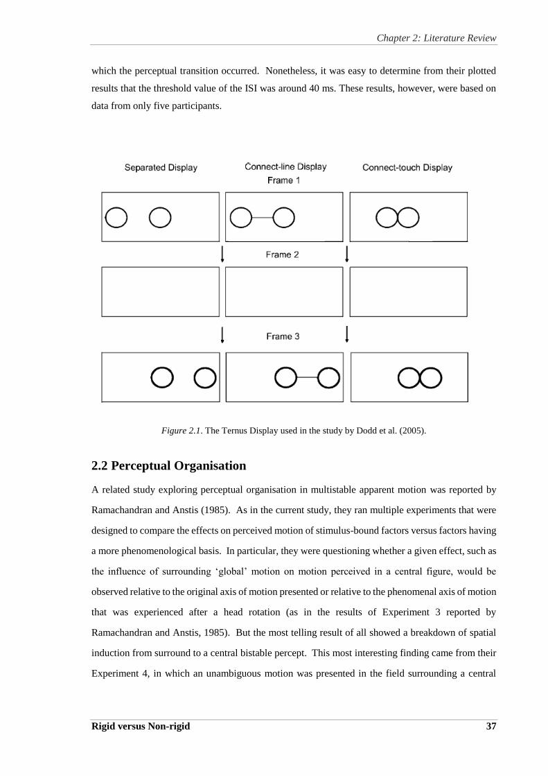
Chapter 2: Literature Review
Rigid versus Non-rigid 37
which the perceptual transition occurred. Nonetheless, it was easy to determine from their plotted
results that the threshold value of the ISI was around 40 ms. These results, however, were based on
data from only five participants.
Figure 2.1. The Ternus Display used in the study by Dodd et al. (2005).
2.2 Perceptual Organisation
A related study exploring perceptual organisation in multistable apparent motion was reported by
Ramachandran and Anstis (1985). As in the current study, they ran multiple experiments that were
designed to compare the effects on perceived motion of stimulus-bound factors versus factors having
a more phenomenological basis. In particular, they were questioning whether a given effect, such as
the influence of surrounding ‘global’ motion on motion perceived in a central figure, would be
observed relative to the original axis of motion presented or relative to the phenomenal axis of motion
that was experienced after a head rotation (as in the results of Experiment 3 reported by
Ramachandran and Anstis, 1985). But the most telling result of all showed a breakdown of spatial
induction from surround to a central bistable percept. This most interesting finding came from their
Experiment 4, in which an unambiguous motion was presented in the field surrounding a central
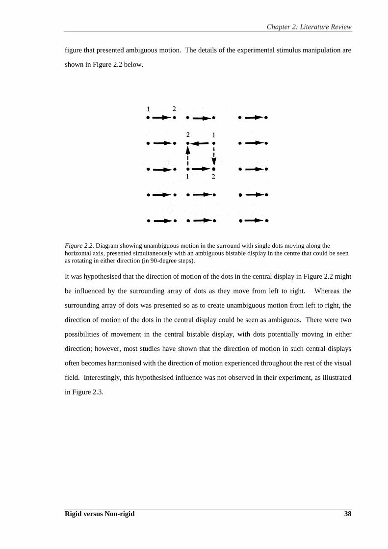
Chapter 2: Literature Review
Rigid versus Non-rigid 38
figure that presented ambiguous motion. The details of the experimental stimulus manipulation are
shown in Figure 2.2 below.
Figure 2.2. Diagram showing unambiguous motion in the surround with single dots moving along the
horizontal axis, presented simultaneously with an ambiguous bistable display in the centre that could be seen
as rotating in either direction (in 90-degree steps).
It was hypothesised that the direction of motion of the dots in the central display in Figure 2.2 might
be influenced by the surrounding array of dots as they move from left to right. Whereas the
surrounding array of dots was presented so as to create unambiguous motion from left to right, the
direction of motion of the dots in the central display could be seen as ambiguous. There were two
possibilities of movement in the central bistable display, with dots potentially moving in either
direction; however, most studies have shown that the direction of motion in such central displays
often becomes harmonised with the direction of motion experienced throughout the rest of the visual
field. Interestingly, this hypothesised influence was not observed in their experiment, as illustrated
in Figure 2.3.
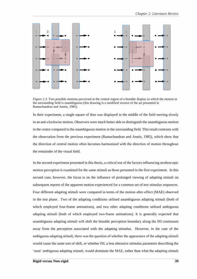
Chapter 2: Literature Review
Rigid versus Non-rigid 39
Figure 2.3. Two possible motions perceived in the central region of a bistable display in which the motion in
the surrounding field is unambiguous (this drawing is a modified version of the art presented in
Ramachandran and Anstis, 1985).
In their experiment, a single square of dots was displayed in the middle of the field moving slowly
in an anti-clockwise motion. Observers were much better able to distinguish the unambiguous motion
in the centre compared to the unambiguous motion in the surrounding field. This result contrasts with
the observation from the previous experiment (Ramachandran and Anstis, 1985), which show that
the direction of central motion often becomes harmonised with the direction of motion throughout
the remainder of the visual field.
In the second experiment presented in this thesis, a critical test of the factors influencing stroboscopic
motion perception is examined for the same stimuli as those presented in the first experiment. In this
second case, however, the focus is on the influence of prolonged viewing of adapting stimuli on
subsequent reports of the apparent motion experienced for a common set of test stimulus sequences.
Four different adapting stimuli were compared in terms of the motion after-effect (MAE) observed
in the test phase. Two of the adapting conditions utilised unambiguous adapting stimuli (both of
which employed four-frame animations), and two other adapting conditions utilised ambiguous
adapting stimuli (both of which employed two-frame animations). It is generally expected that
unambiguous adapting stimuli will shift the bistable perception boundary along the ISI continuum
away from the perception associated with the adapting stimulus. However, in the case of the
ambiguous adapting stimuli, there was the question of whether the appearance of the adapting stimuli
would cause the same sort of shift, or whether ISI, a less obtrusive stimulus parameter describing the
‘seen’ ambiguous adapting stimuli, would dominate the MAE, rather than what the adapting stimuli

Chapter 2: Literature Review
Rigid versus Non-rigid 40
are ‘seen as.’ Thus, the second experiment examined this fundamental distinction between sensory
and cognitive factors, which is what is implied by this terminological distinction between what
stimuli are ‘seen’ versus what stimuli are ‘seen as’ (cf. Anstis and Moulden, 1970).
There is certainly a question about whether ISI is the most appropriate choice for describing and
manipulating stimulus timing in this context. Previous researchers (e.g. Shepard and Judd, 1976)
have chosen to adjust the cycle duration rather than ISI. In contrast, Ramachandran and Anstis (1985)
chose to manipulate stimulus onset asynchrony (SOA) rather than ISI. Their assumption that SOA
was a more critical determinant of apparent motion than ISI was based on conclusions reached by
Kolers (1972). More recent work, however, particularly in studies of the Ternus Illusion (e.g.
Petersik and Pantle, 1979), has emphasised the manipulation of ISI rather than SOA. The reason for
this emphasis on ISI becomes clear when the relative influence of SOA and ISI are examined directly,
as they were in Petersik and Pantle (1979). As the later description of their studies using the display
described by Ternus (1926) makes clear, SOA only appears to be a salient factor in many studies by
virtue of its confounded manipulation with the more potent ISI factor.
Besides SOA, the overall cycle time (or period) of the stimulus sequence is another measure of the
temporal character of the Ternus display that might also be regarded as a potential predictor of the
relative dominance of group versus element movement sensation. Since the period of one complete
animation cycle is the sum total of the two stimulus frame durations (Frame 1 and Frame 2) and the
two ISI durations, this potential predictor confounds these two stimulus parameters. Yet SOA could
feasibly be considered a more global aspect of the stroboscopic display than ISI, in helping to
describe what contributes to the percentage of percepts response from element versus group
movement. Suffice it to say that a comparison of the dependency of the outcome variable on different
combinations of temporal parameters should reveal which is the preferred measure.
In order to clarify the interaction between frame duration, ISI and cycle duration, the data plotted in
Figure 3 in the paper reporting Petersik’s and Pantle’s (1979) original results were replotted here in
Figures 2.4 and 2.5. In Figure 2.4, the x-axis shows the values of the ISI at which stimuli were
presented. On the y-axis are plotted the mean percentages of group movement responses as a function
of ISI with the parameter between the curves being the frame duration values, which were set to
400ms, 200ms and 100ms. The blue triangles are for the frame duration of 400ms, the black squares
are for the frame duration of 200ms and the red circles are for the frame duration of 100ms. This
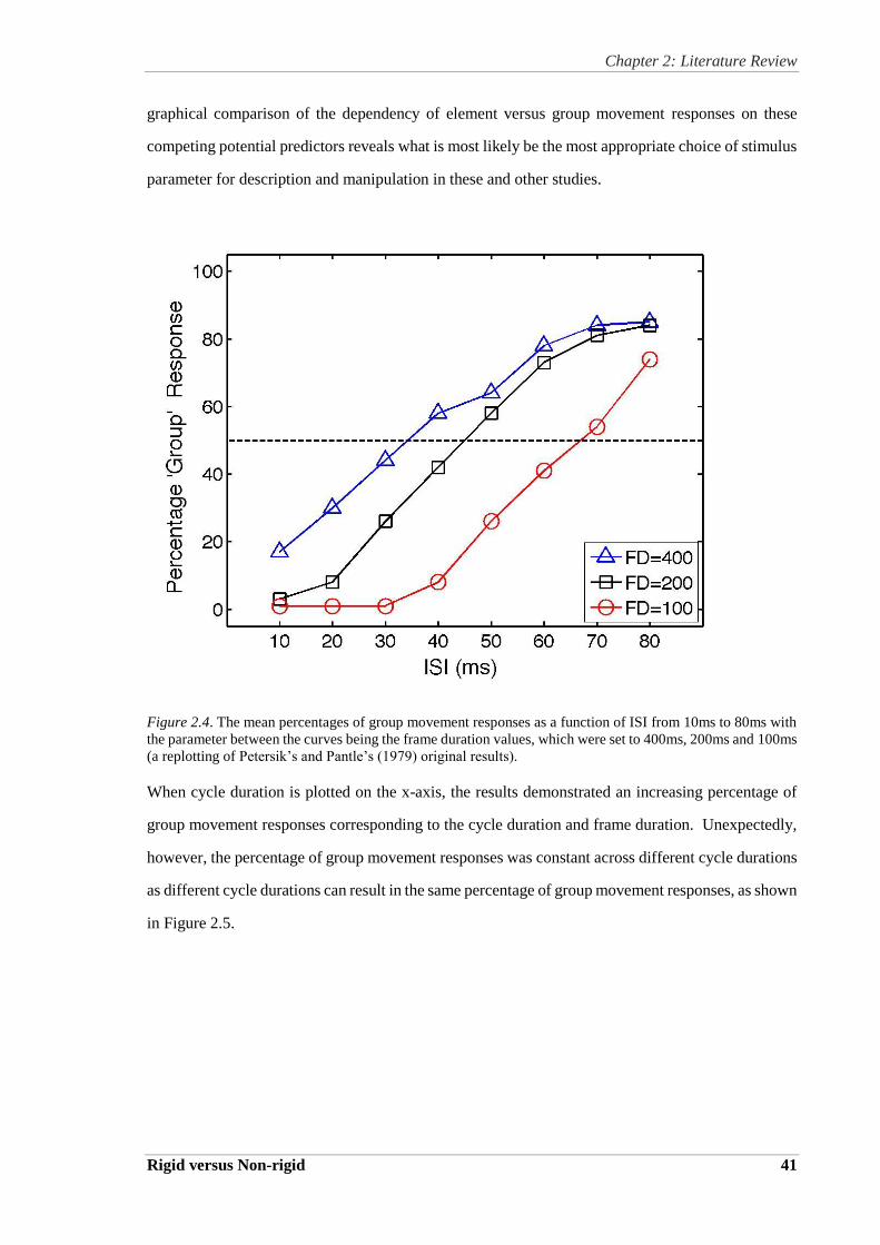
Chapter 2: Literature Review
Rigid versus Non-rigid 41
graphical comparison of the dependency of element versus group movement responses on these
competing potential predictors reveals what is most likely be the most appropriate choice of stimulus
parameter for description and manipulation in these and other studies.
Figure 2.4. The mean percentages of group movement responses as a function of ISI from 10ms to 80ms with
the parameter between the curves being the frame duration values, which were set to 400ms, 200ms and 100ms
(a replotting of Petersik’s and Pantle’s (1979) original results).
When cycle duration is plotted on the x-axis, the results demonstrated an increasing percentage of
group movement responses corresponding to the cycle duration and frame duration. Unexpectedly,
however, the percentage of group movement responses was constant across different cycle durations
as different cycle durations can result in the same percentage of group movement responses, as shown
in Figure 2.5.
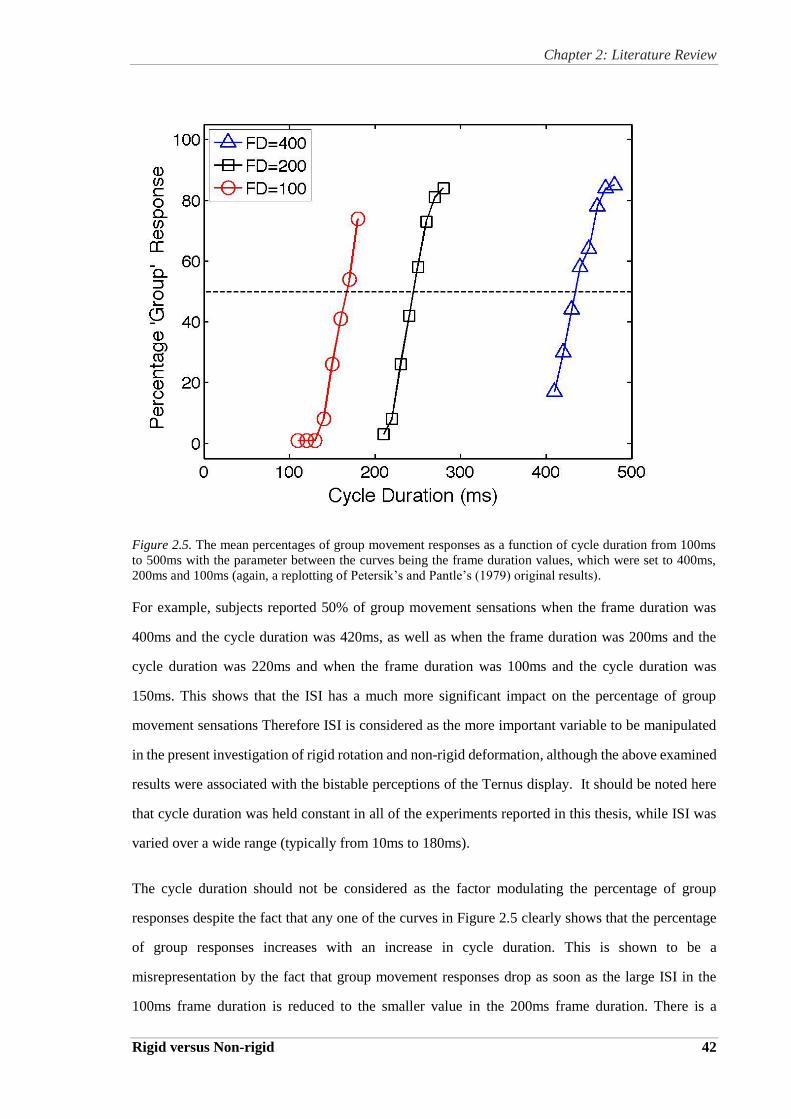
Chapter 2: Literature Review
Rigid versus Non-rigid 42
Figure 2.5. The mean percentages of group movement responses as a function of cycle duration from 100ms
to 500ms with the parameter between the curves being the frame duration values, which were set to 400ms,
200ms and 100ms (again, a replotting of Petersik’s and Pantle’s (1979) original results).
For example, subjects reported 50% of group movement sensations when the frame duration was
400ms and the cycle duration was 420ms, as well as when the frame duration was 200ms and the
cycle duration was 220ms and when the frame duration was 100ms and the cycle duration was
150ms. This shows that the ISI has a much more significant impact on the percentage of group
movement sensations Therefore ISI is considered as the more important variable to be manipulated
in the present investigation of rigid rotation and non-rigid deformation, although the above examined
results were associated with the bistable perceptions of the Ternus display. It should be noted here
that cycle duration was held constant in all of the experiments reported in this thesis, while ISI was
varied over a wide range (typically from 10ms to 180ms).
The cycle duration should not be considered as the factor modulating the percentage of group
responses despite the fact that any one of the curves in Figure 2.5 clearly shows that the percentage
of group responses increases with an increase in cycle duration. This is shown to be a
misrepresentation by the fact that group movement responses drop as soon as the large ISI in the
100ms frame duration is reduced to the smaller value in the 200ms frame duration. There is a
Chapter 2: Literature Review
Rigid versus Non-rigid 43
reversion from a high proportion of group responses to a low proportion of group responses. The
obvious implication is that the ISI value, not the cycle duration, matters most. The cycle duration
only looks like a good explanatory variable because it increases with an increase in the ISI as long
as the frame duration is held constant.
Petersik and Pantle (1979) studied the bistable movement percept under selective adaptation
conditions resulting from prolonged viewing of a stroboscopic stimulus producing predominantly
one or the other of the two movement sensations. For the subsequent test phase, they applied a set
of limiting conditions to the movement displays to determine the relative dominance of the two
movement sensations. For example, in one experiment, they showed that dark adaptation interacted
with the process underlying the element and group movement sensations. They tracked the resulting
percepts using a two-alternative forced-choice task, based on the assumption that the two sensations
were mutually exclusive; that is, the percepts experienced as element movement or group movement
could not be experienced as some combination of the two sensations, but only as one or the other at
a given time. Just as in the case of the perspective reversals in the static Necker Cube, the movement
sensations investigated here interchange automatically and are observed to be alternating between
the two without any intentional shift in the attention of the observer. It was assumed that the
switching between the two motion sensations is caused by the switch between the operation of one
internal visual mechanism and the operation of another. In fact, the two alternatives cannot be
distinguished. Since the perceptual studies reported in this thesis did not attempt to reveal the
operation of underlying neural mechanisms, the neutral term “process” will be used throughout to
refer to the perceptual mechanism or state of activity that causes these two sensations. This term was
chosen to avoid commitment to a specific interpretation. Suffice it to say that the overwhelming
view in the literature is that only one of these two processes will operate at any given time.
Assuming the two-process hypothesis will continue to be supported by the results of related studies,
it is also assumed that adaptation to a stimulus producing a strong element movement sensation
should weaken the response of the process mediating the element movement sensation more than the
process mediating the group movement sensation, thus increasing the proportion of group movement
sensations reported after the adaptation period This is a perspective that is generally held to describe
most motion after-effects; that is, adaptation to a stimulus producing one sensation increases the
proportion of responses for the complementary sensation associated with a competing process.

Chapter 2: Literature Review
Rigid versus Non-rigid 44
In order to explain the selection of variables to be manipulated in the two experiments presented in
this thesis, the following discussion examines some of the competing variables from previous studies.
Consistent with the above two-process hypothesis, the results found in one of the experiments
reported by Petersik and Pantle (1979) showed that, as the ISI increases, all three curves showed an
increase in group movement (i.e. in the control condition, after adaptation to element movement and
after adaptation to group movement). In their subsequent experiment, the results showed that frame
duration had a significant impact. Both frame duration and ISI have been demonstrated in other
research to significantly increase the percentage of group movement responses. In relation to
correlation between frame duration and ISI for the generation of group and element movement
sensations, Petersik and Pantle (1979) concluded from analysis of variance that the interaction of
frame duration and ISI has a significant impact, but the effects of both are not additive.
Kubovy and Gepshtein (2003) presented empirical and theoretical findings on grouping in space and
in spacetime. They argued that perceptual organisation is a semi-voluntary process that occurs on the
boundary between experience of the world and unconscious perceptual processing. For example,
when a Necker cube is first seen, the perspective view depends on the point of fixation. Changing
the point of visual fixation makes it possible to control our three-dimensional interpretation of the
two-dimensional image. The first two studies by Kubovy and Gepshtein (2003) showed that grouping
by proximity could be modelled with a few characteristics according to a Gestalt phenomenon and
the relation between grouping by spatial proximity and grouping by spatiotemporal proximity. They
did not discuss the possibility of decomposing motion processing into two operations, such as
grouping by spatial proximity and grouping by spatiotemporal proximity. These two principles
describing the resolution of corresponding components may be difficult for the reader to grasp
outside the context of the discussion presented in Kubovy and Gepshtein (2003). Suffice it to say
here that spatial proximity operating alone can only associate local component details, but
spatiotemporal proximity can associate component details on a more global level, which takes both
spatial and temporal factors into consideration, allowing more global resolution such as that
underlying rigid rotation. These two processes describe how corresponding components such as box
corners can be matched in various types of apparent motion.
As was described above, Shepard and Judd (1976) presented two images of a three-dimensional
object in rapid alternation, which resulted in the perception of an object rotating in depth. However,
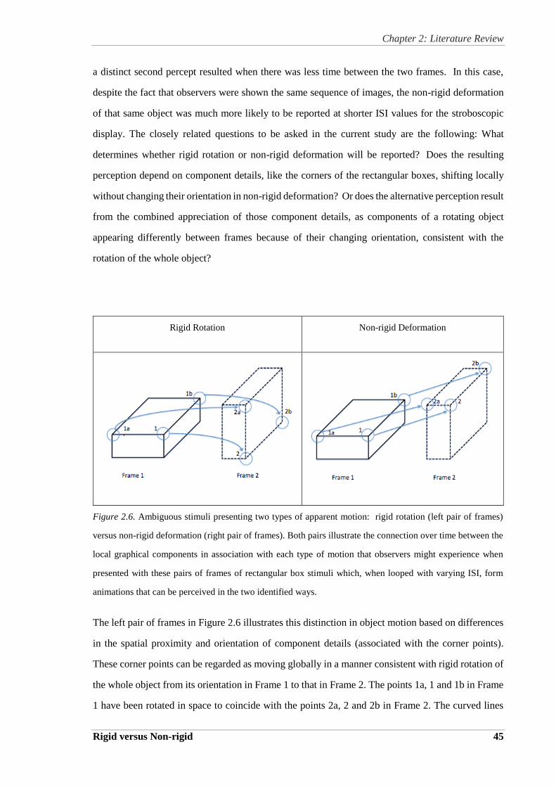
Chapter 2: Literature Review
Rigid versus Non-rigid 45
a distinct second percept resulted when there was less time between the two frames. In this case,
despite the fact that observers were shown the same sequence of images, the non-rigid deformation
of that same object was much more likely to be reported at shorter ISI values for the stroboscopic
display. The closely related questions to be asked in the current study are the following: What
determines whether rigid rotation or non-rigid deformation will be reported? Does the resulting
perception depend on component details, like the corners of the rectangular boxes, shifting locally
without changing their orientation in non-rigid deformation? Or does the alternative perception result
from the combined appreciation of those component details, as components of a rotating object
appearing differently between frames because of their changing orientation, consistent with the
rotation of the whole object?
Rigid Rotation Non-rigid Deformation
Figure 2.6. Ambiguous stimuli presenting two types of apparent motion: rigid rotation (left pair of frames)
versus non-rigid deformation (right pair of frames). Both pairs illustrate the connection over time between the
local graphical components in association with each type of motion that observers might experience when
presented with these pairs of frames of rectangular box stimuli which, when looped with varying ISI, form
animations that can be perceived in the two identified ways.
The left pair of frames in Figure 2.6 illustrates this distinction in object motion based on differences
in the spatial proximity and orientation of component details (associated with the corner points).
These corner points can be regarded as moving globally in a manner consistent with rigid rotation of
the whole object from its orientation in Frame 1 to that in Frame 2. The points 1a, 1 and 1b in Frame
1 have been rotated in space to coincide with the points 2a, 2 and 2b in Frame 2. The curved lines
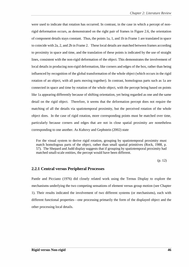
Chapter 2: Literature Review
Rigid versus Non-rigid 46
were used to indicate that rotation has occurred. In contrast, in the case in which a percept of non-
rigid deformation occurs, as demonstrated on the right pair of frames in Figure 2.6, the orientation
of component details stays constant. Thus, the points 1a, 1, and 1b in Frame 1 are translated in space
to coincide with 2a, 2, and 2b in Frame 2. These local details are matched between frames according
to proximity in space and time, and the translation of these points is indicated by the use of straight
lines, consistent with the non-rigid deformation of the object. This demonstrates the involvement of
local details in producing non-rigid deformation, like corners and edges of the box, rather than being
influenced by recognition of the global transformation of the whole object (which occurs in the rigid
rotation of an object, with all parts moving together). In contrast, homologous parts such as 1a are
connected in space and time by rotation of the whole object, with the percept being based on points
like 1a appearing differently because of shifting orientation, yet being regarded as one and the same
detail on the rigid object. Therefore, it seems that the deformation percept does not require the
matching of all the details via spatiotemporal proximity, but the perceived rotation of the whole
object does. In the case of rigid rotation, more corresponding points must be matched over time,
particularly because corners and edges that are not in close spatial proximity are nonetheless
corresponding to one another. As Kubovy and Gephstein (2002) state
For the visual system to derive rigid rotation, grouping by spatiotemporal proximity must
match homologous parts of the object, rather than small spatial primitives (Rock, 1988, p.
57). The Shepard and Judd display suggests that if grouping by spatiotemporal proximity had
matched small-scale entities, the percept would have been different.
(p. 12)
2.2.1 Central versus Peripheral Processes
Pantle and Picciano (1976) did closely related work using the Ternus Display to explore the
mechanisms underlying the two competing sensations of element versus group motion (see Chapter
1). Their results indicated the involvement of two different systems (or mechanisms), each with
different functional properties—one processing primarily the form of the displayed object and the
other processing local details.
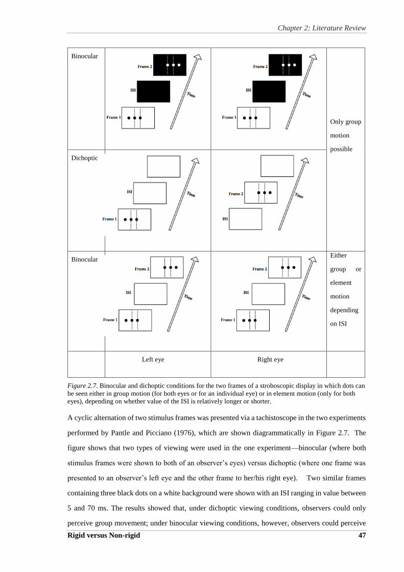
Chapter 2: Literature Review
Rigid versus Non-rigid 47
Binocular
Only group
motion
possible
Dichoptic
Binocular
Either
group or
element
motion
depending
on ISI
Left eye Right eye
Figure 2.7. Binocular and dichoptic conditions for the two frames of a stroboscopic display in which dots can
be seen either in group motion (for both eyes or for an individual eye) or in element motion (only for both
eyes), depending on whether value of the ISI is relatively longer or shorter.
A cyclic alternation of two stimulus frames was presented via a tachistoscope in the two experiments
performed by Pantle and Picciano (1976), which are shown diagrammatically in Figure 2.7. The
figure shows that two types of viewing were used in the one experiment—binocular (where both
stimulus frames were shown to both of an observer’s eyes) versus dichoptic (where one frame was
presented to an observer’s left eye and the other frame to her/his right eye). Two similar frames
containing three black dots on a white background were shown with an ISI ranging in value between
5 and 70 ms. The results showed that, under dichoptic viewing conditions, observers could only
perceive group movement; under binocular viewing conditions, however, observers could perceive

Chapter 2: Literature Review
Rigid versus Non-rigid 48
both element movement and group movement. In addition, observers reported element movement
most frequently at short ISI values (e.g., ISIs less than 40 ms). The transition from reports of element
movement to those of group movement occurred at around 40 ms, and observers reported
predominantly group movement at the longer ISI values (e.g., ISIs greater than 40 ms).
In the second experiment, Pantle and Picciano (1976) manipulated the polarity of the stimulus
contrast using two different stimulus displays. In one condition, the contrast was positive (black dots
on a white background in both stimulus frames); in the other, the contrast was reversed from positive
to negative (one frame containing black dots on a white background and another frame containing
white dots on a black background). Between the two stimulus frames, the visual field was completely
dark for the duration of the ISI, which varied from 10 to 80 ms. Under the positive-positive viewing
condition, the results were similar to those under the binocular condition; under the positive-negative
condition. However, observers reported predominantly group movement regardless of the ISI value.
This requires a more thorough discussion. In the positive-negative condition, there is no local match;
corresponding points do not match each other because one frame is positive and the other is negative.
That defeats the response of element motion. At the peripheral level, the two eyes do not interact
with each other, nor does the information from the two stimulus frames interact or combine.
Observers only see the corresponding features, such as the corners and edges in the image, but they
detect the forms and shapes in the cortex since they can be compared at the central level. The is about
seeing shapes, not motion (Fine et al., 2003; Larsson and Heeger, 2006), so the process is more likely
to be influenced by forms and shapes whereas at the peripheral level it is more likely to detect the
local motion without forms. This is because, locally, the observer only needs to see the corresponding
elements so the motion can be detected without seeing forms. The important point is that detecting
local motion does not require the detection of form, as described in an earlier study by Exner (1888).
His findings show that the observer can see the motion of a spark as it moves from one location to
another location without recognising the two locations—in effect, without recognising the spatial
offset between the two sparks.
This phenomenon is similar to that of element motion, in that the seen motion occurs without
recognition of the overall form. When the overall form is recognised, the apparent movement called
group motion occurs, and this must result from a central process since it was not possible to see such
group motion at short ISI values in the binocular viewing condition. Of course, when the ISI grows
Chapter 2: Literature Review
Rigid versus Non-rigid 49
much longer (greater than 40ms) in the binocular viewing condition, then the form can be recognised,
and the observer’s percepts will shift away from the local motion associated with element movement
towards group movement. These observations about element and group movement foreshadow the
treatment of the non-rigid deformation and rigid rotation to be addressed in this thesis.
The multistability phenomenon suggests that two different motion systems operate in the visual
system. It indicates that observers perceive group movement at longer ISI values because the group
movement signal is processed centrally rather than peripherally. Furthermore, it takes more time for
this central process since the visual system needs to combine information from both eyes. Of course,
some type of form processing occurs peripherally so that, at the retina of each individual eye, some
local components are detected and matched so as to generate the element movement, but this
possibility disappears when the two stimulus frames have a contrast reversal, as the local components
do not strictly match in this case. This shows that the relative intensity of points in the two stimulus
frames was important to the observer’s perception of element movement. The element motion cannot
be generated from the local form when contrast is reversed; therefore, it must be the global form of
the dots displayed that is primarily responsible for the generation of group movement, which was
understood to be based on central processing. In other words, the local correspondence at short ISI
values relies on simple local matching in one eye, which can only function in the binocular and not
the dichoptic condition. This is because in the dichoptic condition there is no local interaction in one
eye between the two stimulus frames (as one stimulus frame is perceived in one eye and the other
stimulus frame is perceived later in the other eye).
2.3 Studies of Motion After-effect (MAE)
Anstis and Moulden (1970) conducted three experiments to determine whether the movement of
MAE is central or peripheral. Their aim was to find out if the MAE is caused by the adaptation of
some central mechanism. The crucial experiment they conducted was to separate two eyes to view
the rotating object. The first experiment, demonstrated in Figure 2.8 (a), was to let the left eye view
a sectored disc rotating to the left, and the right eye to view a disc rotating in the opposite direction.

Chapter 2: Literature Review
Rigid versus Non-rigid 50
Left Eye
Stimulation
Right Eye
Stimulation
Conclusion
Motion After-
effect (MAE)
Left Eye: Rotating
to the right.
Right Eye:
Rotating to the left.
Therefore,
Retinal
(Peripheral)
B i n o c u l a r
Presentation
Both eyes open No MAE
D i c h o p t i c
Presentation
With each eye in rapid alternation MAE to that eye
M o n o c u l a r
Presentation
Only one eye open MAE to that eye
Figure 2.8 (a). Experiment one.
The second experiment, illustrated in Figure 2.8 (b), was to separate out the movement information
from the two eyes by using a ring of lights that switched on and off to produce a rotating movement.
The six bulbs were set up in a circle to rotate anti-clockwise. The first and third frames were fed to
the left eye then the second and fourth frames were fed to the right eye. The sequence was repeated
by the display program. The results showed that both eyes together saw rotation anticlockwise but
each eye on its own saw a random flashing oscillation. Therefore, the author inferred the involvement
of central activity in the MAE for this case.
Chapter 2: Literature Review
Rigid versus Non-rigid 51
Figure 2.8. (b). Experiment 2
The third experiment, illustrated in Figure 2.8 (c), induced each eye to see clockwise movement, but
the two eyes together saw that movement as anticlockwise. Eight bulbs in a circle were used to alter
the order in which the lights were switched on and off. Eight bulbs were first flashed simultaneously
to the left eye; then the eight next to them flashed in an anti-clockwise direction to the right eye, then
the next eight to the left eye, followed by another eight to the right eye and so on. The results showed
that, after monocular viewing, the subsequence of viewing a stationary field with the same eye caused
an anti-clockwise MAE, but after dichoptic viewing, the subsequence of viewing a stationary field
with both eyes reported a clockwise MAE. Therefore, the activity of MAE must be based on a central
process, as a clockwise MAE was seen; otherwise each eye should have seen anticlockwise
movement on its own according to the processing based on peripheral components.
Experiment 2
Left Eye
Stimulation
Right Eye
Stimulation
Conclusion
Motion After-
effect (MAE)
A clockwise
MAE.
Central fusion from
the two eyes.
Binocular
Presentation
All four frames fed to both eyes, flashed in
anti-clockwise sequence.
A clock-wise
MAE.
Dichoptic
Presentation
Fed to the left and right alternatively
i) Monocular viewing
Ambiguous
stimulus.
No MAE.
ii) Dichoptic viewing A clock-wise
MAE.
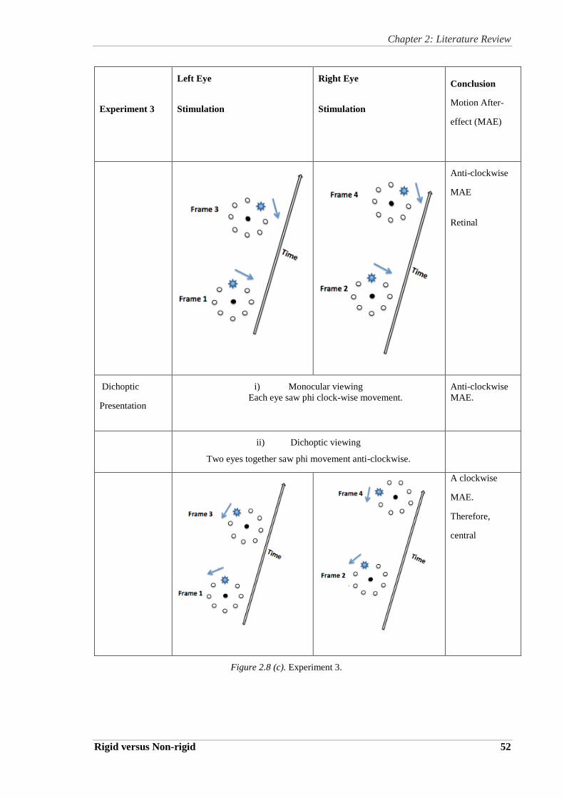
Chapter 2: Literature Review
Rigid versus Non-rigid 52
Experiment 3
Left Eye
Stimulation
Right Eye
Stimulation
Conclusion
Motion After-
effect (MAE)
vie
Anti-clockwise
MAE
Retinal
Dichoptic
Presentation
i) Monocular viewing
Each eye saw phi clock-wise movement.
Anti-clockwise
MAE.
ii) Dichoptic viewing
Two eyes together saw phi movement anti-clockwise.
A clockwise
MAE.
Therefore,
central
Figure 2.8 (c). Experiment 3.
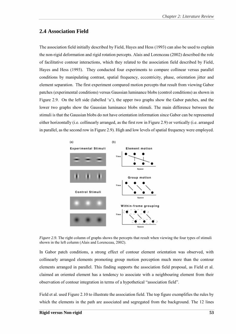
Chapter 2: Literature Review
Rigid versus Non-rigid 53
2.4 Association Field
The association field initially described by Field, Hayes and Hess (1993) can also be used to explain
the non-rigid deformation and rigid rotation percepts. Alais and Lorenceau (2002) described the role
of facilitative contour interactions, which they related to the association field described by Field,
Hayes and Hess (1993). They conducted four experiments to compare collinear versus parallel
conditions by manipulating contrast, spatial frequency, eccentricity, phase, orientation jitter and
element separation. The first experiment compared motion percepts that result from viewing Gabor
patches (experimental conditions) versus Gaussian luminance blobs (control conditions) as shown in
Figure 2.9. On the left side (labelled ‘a’), the upper two graphs show the Gabor patches, and the
lower two graphs show the Gaussian luminance blobs stimuli. The main difference between the
stimuli is that the Gaussian blobs do not have orientation information since Gabor can be represented
either horizontally (i.e. collinearly arranged, as the first row in Figure 2.9) or vertically (i.e. arranged
in parallel, as the second row in Figure 2.9). High and low levels of spatial frequency were employed.
Figure 2.9. The right column of graphs shows the percepts that result when viewing the four types of stimuli
shown in the left column (Alais and Lorenceau, 2002).
In Gabor patch conditions, a strong effect of contour element orientation was observed, with
collinearly arranged elements promoting group motion perception much more than the contour
elements arranged in parallel. This finding supports the association field proposal, as Field et al.
claimed an oriented element has a tendency to associate with a neighbouring element from their
observation of contour integration in terms of a hypothetical “association field”.
Field et al. used Figure 2.10 to illustrate the association field. The top figure exemplifies the rules by
which the elements in the path are associated and segregated from the background. The 12 lines
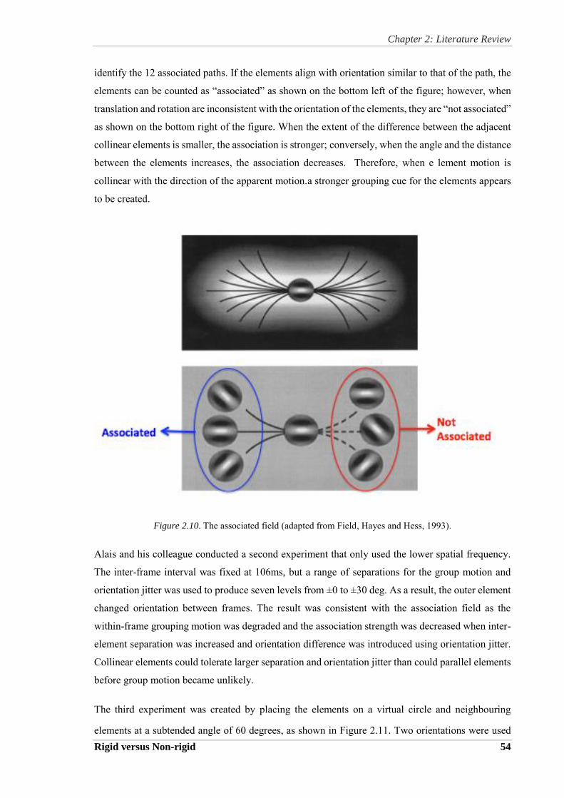
Chapter 2: Literature Review
Rigid versus Non-rigid 54
identify the 12 associated paths. If the elements align with orientation similar to that of the path, the
elements can be counted as “associated” as shown on the bottom left of the figure; however, when
translation and rotation are inconsistent with the orientation of the elements, they are “not associated”
as shown on the bottom right of the figure. When the extent of the difference between the adjacent
collinear elements is smaller, the association is stronger; conversely, when the angle and the distance
between the elements increases, the association decreases. Therefore, when e lement motion is
collinear with the direction of the apparent motion.a stronger grouping cue for the elements appears
to be created.
Figure 2.10. The associated field (adapted from Field, Hayes and Hess, 1993).
Alais and his colleague conducted a second experiment that only used the lower spatial frequency.
The inter-frame interval was fixed at 106ms, but a range of separations for the group motion and
orientation jitter was used to produce seven levels from ±0 to ±30 deg. As a result, the outer element
changed orientation between frames. The result was consistent with the association field as the
within-frame grouping motion was degraded and the association strength was decreased when inter-
element separation was increased and orientation difference was introduced using orientation jitter.
Collinear elements could tolerate larger separation and orientation jitter than could parallel elements
before group motion became unlikely.
The third experiment was created by placing the elements on a virtual circle and neighbouring
elements at a subtended angle of 60 degrees, as shown in Figure 2.11. Two orientations were used

Chapter 2: Literature Review
Rigid versus Non-rigid 55
as the stimuli—the orthogonal as the parallel condition on the left column and the aligned as the
collinear condition. The results of this experiment supported those of the second experiment. The
strong collinear facilitation occurred for a circular arrangement where the orientation difference
between elements is 60 degrees, and the correct connection between elements decreases as the path
angle increases because the incorrect matches become more possible. The last experiment was tested
based on the eccentricity of 1, 6, and 12 degrees when collinear and parallel conditions of the linear
Ternus were compared. It was shown that overall level of group motion for both conditions decreased
with eccentricity and the parallel condition benefitted from facilitative lateral interactions. Overall,
the study confirmed the role of oriented association fields in apparent motion.
Figure 2.11. Stimulus for experiment 3 (Alais and Lorenceau, 2002).
The study by Alais and Lorenceau (2002) also compared predictions based on the association field
account of contour investigation which posits the existence in the cortex of units that perform ‘second
order’ orientational filtering. Proponents of this view believe that the first-order oriented filters in
simple cortical cells are ‘tributary’ units that deliver input to these second-order oriented filters.
These speculations regarding the underlying visual neuroscience are not addressed in this thesis, as
they are beyond the scope of the current research. Nonetheless, it is of interest to examine the results
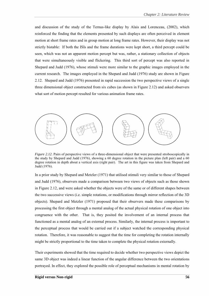
Chapter 2: Literature Review
Rigid versus Non-rigid 56
and discussion of the study of the Ternus-like display by Alais and Lorenceau, (2002), which
reinforced the finding that the elements presented by such displays are often perceived in element
motion at short frame rates and in group motion at long frame rates. However, their display was not
strictly bistable: If both the ISIs and the frame durations were kept short, a third percept could be
seen, which was not an apparent motion percept but was, rather, a stationary collection of objects
that were simultaneously visible and flickering. This third sort of percept was also reported in
Shepard and Judd (1976), whose stimuli were more similar to the graphic images employed in the
current research. The images employed in the Shepard and Judd (1976) study are shown in Figure
2.12. Shepard and Judd (1976) presented in rapid succession the two perspective views of a single
three dimensional object constructed from six cubes (as shown in Figure 2.12) and asked observers
what sort of motion percept resulted for various animation frame rates.
Figure 2.12. Pairs of perspective views of a three-dimensional object that were presented stroboscopically in
the study by Shepard and Judd (1976), showing a 60 degree rotation in the picture plan (left pair) and a 60
degree rotation in depth about a vertical axis (right pair). The art in this figure was taken from Shepard and
Judd (1976).
In a prior study by Shepard and Metzler (1971) that utilised stimuli very similar to those of Shepard
and Judd (1976), observers made a comparison between two views of objects such as those shown
in Figure 2.12, and were asked whether the objects were of the same or of different shapes between
the two successive views (i.e. simple rotations, or modifications through mirror reflection of the 3D
objects). Shepard and Metzler (1971) proposed that their observers made these comparisons by
processing the first object through a mental analog of the actual physical rotation of one object into
congruence with the other. That is, they posited the involvement of an internal process that
functioned as a mental analog of an external process. Similarly, the internal process is important to
the perceptual process that would be carried out if a subject watched the corresponding physical
rotation. Therefore, it was reasonable to suggest that the time for completing the rotation internally
might be strictly proportional to the time taken to complete the physical rotation externally.
Their experiments showed that the time required to decide whether two perspective views depict the
same 3D object was indeed a linear function of the angular difference between the two orientations
portrayed. In effect, they explored the possible role of perceptual mechanisms in mental rotation by
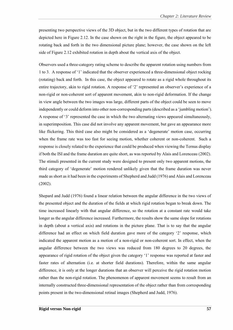
Chapter 2: Literature Review
Rigid versus Non-rigid 57
presenting two perspective views of the 3D object, but in the two different types of rotation that are
depicted here in Figure 2.12. In the case shown on the right in the figure, the object appeared to be
rotating back and forth in the two dimensional picture plane; however, the case shown on the left
side of Figure 2.12 exhibited rotation in depth about the vertical axis of the object.
Observers used a three-category rating scheme to describe the apparent rotation using numbers from
1 to 3. A response of ‘1’ indicated that the observer experienced a three-dimensional object rocking
(rotating) back and forth. In this case, the object appeared to rotate as a rigid whole throughout its
entire trajectory, akin to rigid rotation. A response of ‘2’ represented an observer’s experience of a
non-rigid or non-coherent sort of apparent movement, akin to non-rigid deformation. If the change
in view angle between the two images was large, different parts of the object could be seen to move
independently or could deform into other non-corresponding parts (described as a ‘jumbling motion’).
A response of ‘3’ represented the case in which the two alternating views appeared simultaneously,
in superimposition. This case did not involve any apparent movement, but gave an appearance more
like flickering. This third case also might be considered as a ‘degenerate’ motion case, occurring
when the frame rate was too fast for seeing motion, whether coherent or non-coherent. Such a
response is closely related to the experience that could be produced when viewing the Ternus display
if both the ISI and the frame duration are quite short, as was reported by Alais and Lorenceau (2002).
The stimuli presented in the current study were designed to present only two apparent motions, the
third category of ‘degenerate’ motion rendered unlikely given that the frame duration was never
made as short as it had been in the experiments of Shepherd and Judd (1976) and Alais and Lorenceau
(2002).
Shepard and Judd (1976) found a linear relation between the angular difference in the two views of
the presented object and the duration of the fields at which rigid rotation began to break down. The
time increased linearly with that angular difference, so the rotation at a constant rate would take
longer as the angular difference increased. Furthermore, the results show the same slope for rotations
in depth (about a vertical axis) and rotations in the picture plane. That is to say that the angular
difference had an effect on which field duration gave more of the category ‘2’ response, which
indicated the apparent motion as a motion of a non-rigid or non-coherent sort. In effect, when the
angular difference between the two views was reduced from 180 degrees to 20 degrees, the
appearance of rigid rotation of the object given the category ‘1’ response was reported at faster and
faster rates of alternation (i.e. at shorter field durations). Therefore, within the same angular
difference, it is only at the longer durations that an observer will perceive the rigid rotation motion
rather than the non-rigid rotation. The phenomenon of apparent movement seems to result from an
internally constructed three-dimensional representation of the object rather than from corresponding
points present in the two-dimensional retinal images (Shepherd and Judd, 1976).
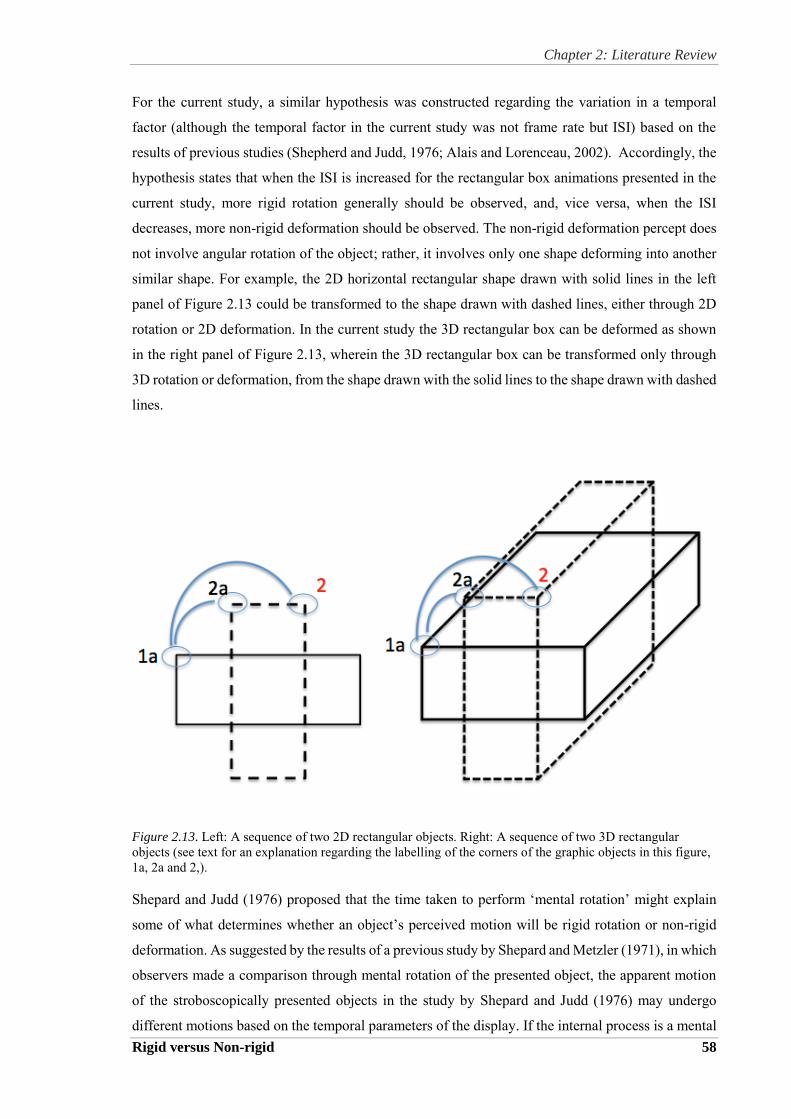
Chapter 2: Literature Review
Rigid versus Non-rigid 58
For the current study, a similar hypothesis was constructed regarding the variation in a temporal
factor (although the temporal factor in the current study was not frame rate but ISI) based on the
results of previous studies (Shepherd and Judd, 1976; Alais and Lorenceau, 2002). Accordingly, the
hypothesis states that when the ISI is increased for the rectangular box animations presented in the
current study, more rigid rotation generally should be observed, and, vice versa, when the ISI
decreases, more non-rigid deformation should be observed. The non-rigid deformation percept does
not involve angular rotation of the object; rather, it involves only one shape deforming into another
similar shape. For example, the 2D horizontal rectangular shape drawn with solid lines in the left
panel of Figure 2.13 could be transformed to the shape drawn with dashed lines, either through 2D
rotation or 2D deformation. In the current study the 3D rectangular box can be deformed as shown
in the right panel of Figure 2.13, wherein the 3D rectangular box can be transformed only through
3D rotation or deformation, from the shape drawn with the solid lines to the shape drawn with dashed
lines.
Figure 2.13. Left: A sequence of two 2D rectangular objects. Right: A sequence of two 3D rectangular
objects (see text for an explanation regarding the labelling of the corners of the graphic objects in this figure,
1a, 2a and 2,).
Shepard and Judd (1976) proposed that the time taken to perform ‘mental rotation’ might explain
some of what determines whether an object’s perceived motion will be rigid rotation or non-rigid
deformation. As suggested by the results of a previous study by Shepard and Metzler (1971), in which
observers made a comparison through mental rotation of the presented object, the apparent motion
of the stroboscopically presented objects in the study by Shepard and Judd (1976) may undergo
different motions based on the temporal parameters of the display. If the internal process is a mental

Chapter 2: Literature Review
Rigid versus Non-rigid 59
analog of an external process, the internal process that takes less time to complete likely will occur
at the shorter ISI values, while the more time-consuming process corresponding to rotation will be
allowed by the longer ISI values. As will be seen in the following chapters of this thesis, the current
experiments have been designed to reveal conditions under which longer ISIs promote the perception
of rigid rotation while the shorter ISIs promote the perception of non-rigid deformation. Some initial
exploration of possible stimulus transformations is in order here. As shown in the left panel of Figure
2.13, if the box’s corner labelled 1a moves to the position labelled 2a, then the 2D rectangular box
could simply be regarded as undergoing non-rigid deformation; however, when corner 1a moves to
corner 2, the type of motion is described as rigid rotation. The factor that may be important in what
is most often perceived here is the amount of distance travelled by the matching corners. Note that
the distance from 1a to 2a is much shorter than the distance from 1a to 2. Thus, it may be that a
longer ISI will be required for the perception of rigid rotation to occur, due to the greater distances
that the corners must travel at a putative fixed speed. The 3D objects shown in the right panel of
Figure 2.13 should behave similarly, and prediction of perceived motion are possible based upon
results of the closely related study of Shepard and Judd (1976). For the current study, stimuli were
constructed that should provide the possibility of two competing motions for the observers. The non-
rigid deformation motion could be described as similar to element motion since the elements shift
individually to spatially close positions. But the rigid rotation motion could be described as similar
to group motion, since the combined elements must move in a coordinated fashion for rigid rotation
of the object to occur. Also, the type of each corresponding corner must be allowed to change
between frames in rigid rotation, as will be explained in reference to Figure 2.13.
In Figure 2.13, the corner labelled 1a can travel from its positions in the first frame to one of two
positions in the second frame, either 2a or 2. If it travels to the position labelled 2a, then its type is
still the same, identified herein as an “external” corner. However, when it travels to the position
labelled 2, then its type is changed to a different sort, identified herein as an “internal” corner (as
discussed in Section 1.4.3 of Chapter 1 in this thesis, and originally described as a “fork” versus an
“arrow” vertex by in Biederman, 1987). So, in addition to this corner travelling further through space
in rigid rotation there is this additional potential reason that the perception of rigid rotation might
require more time to develop than non-rigid deformation. It may be easier for the visual system to
associate corner 1a with corner 2a, in effect, without much internal processing. The rigid rotation,
however, involves matching between an internal corner and an outer corner with different orientation,
which is required by the group motion of the whole constellation of elements.
Ledgeway, Hess and Geisler (2005) found that local orientations and motions are grouped across
space to define simple contours and suggested that orientation cues and motion cues can be applied
by different rules of association. Specifically, they found that when the constituent element directions
are aligned along the axis of the contour, motion-defined contours of moderate curvature are more
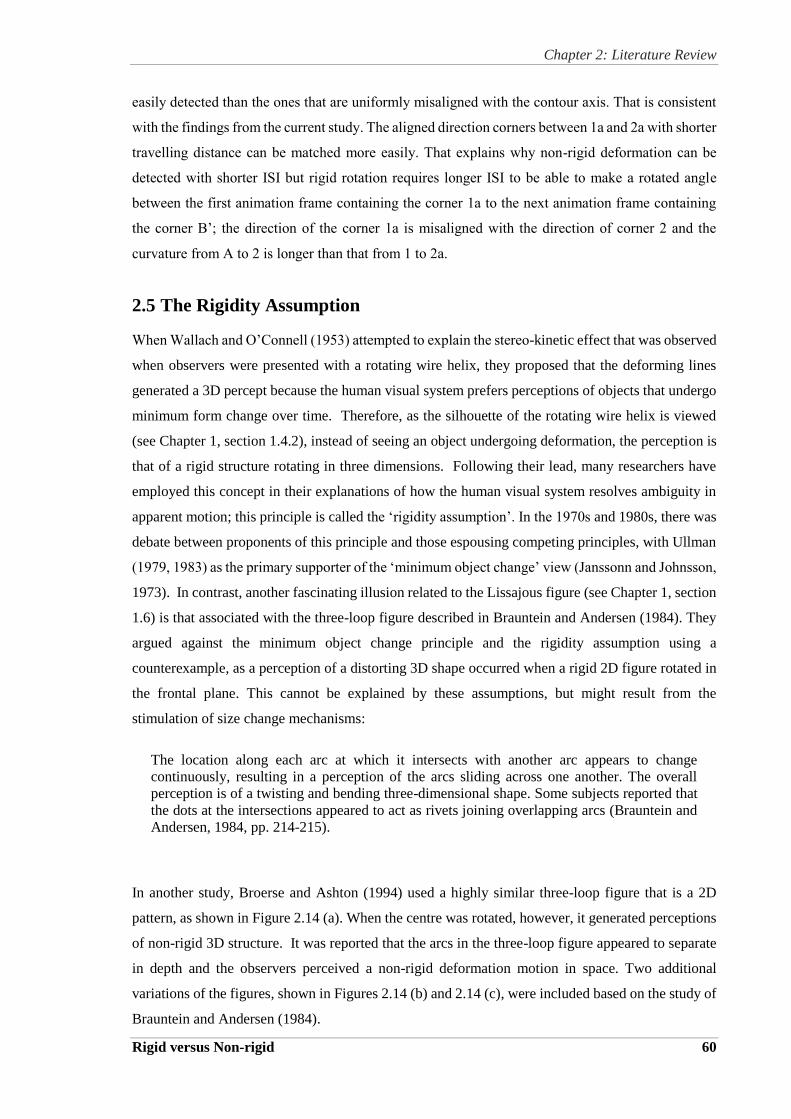
Chapter 2: Literature Review
Rigid versus Non-rigid 60
easily detected than the ones that are uniformly misaligned with the contour axis. That is consistent
with the findings from the current study. The aligned direction corners between 1a and 2a with shorter
travelling distance can be matched more easily. That explains why non-rigid deformation can be
detected with shorter ISI but rigid rotation requires longer ISI to be able to make a rotated angle
between the first animation frame containing the corner 1a to the next animation frame containing
the corner B’; the direction of the corner 1a is misaligned with the direction of corner 2 and the
curvature from A to 2 is longer than that from 1 to 2a.
2.5 The Rigidity Assumption
When Wallach and O’Connell (1953) attempted to explain the stereo-kinetic effect that was observed
when observers were presented with a rotating wire helix, they proposed that the deforming lines
generated a 3D percept because the human visual system prefers perceptions of objects that undergo
minimum form change over time. Therefore, as the silhouette of the rotating wire helix is viewed
(see Chapter 1, section 1.4.2), instead of seeing an object undergoing deformation, the perception is
that of a rigid structure rotating in three dimensions. Following their lead, many researchers have
employed this concept in their explanations of how the human visual system resolves ambiguity in
apparent motion; this principle is called the ‘rigidity assumption’. In the 1970s and 1980s, there was
debate between proponents of this principle and those espousing competing principles, with Ullman
(1979, 1983) as the primary supporter of the ‘minimum object change’ view (Janssonn and Johnsson,
1973). In contrast, another fascinating illusion related to the Lissajous figure (see Chapter 1, section
1.6) is that associated with the three-loop figure described in Brauntein and Andersen (1984). They
argued against the minimum object change principle and the rigidity assumption using a
counterexample, as a perception of a distorting 3D shape occurred when a rigid 2D figure rotated in
the frontal plane. This cannot be explained by these assumptions, but might result from the
stimulation of size change mechanisms:
The location along each arc at which it intersects with another arc appears to change
continuously, resulting in a perception of the arcs sliding across one another. The overall
perception is of a twisting and bending three-dimensional shape. Some subjects reported that
the dots at the intersections appeared to act as rivets joining overlapping arcs (Brauntein and
Andersen, 1984, pp. 214-215).
In another study, Broerse and Ashton (1994) used a highly similar three-loop figure that is a 2D
pattern, as shown in Figure 2.14 (a). When the centre was rotated, however, it generated perceptions
of non-rigid 3D structure. It was reported that the arcs in the three-loop figure appeared to separate
in depth and the observers perceived a non-rigid deformation motion in space. Two additional
variations of the figures, shown in Figures 2.14 (b) and 2.14 (c), were included based on the study of
Brauntein and Andersen (1984).
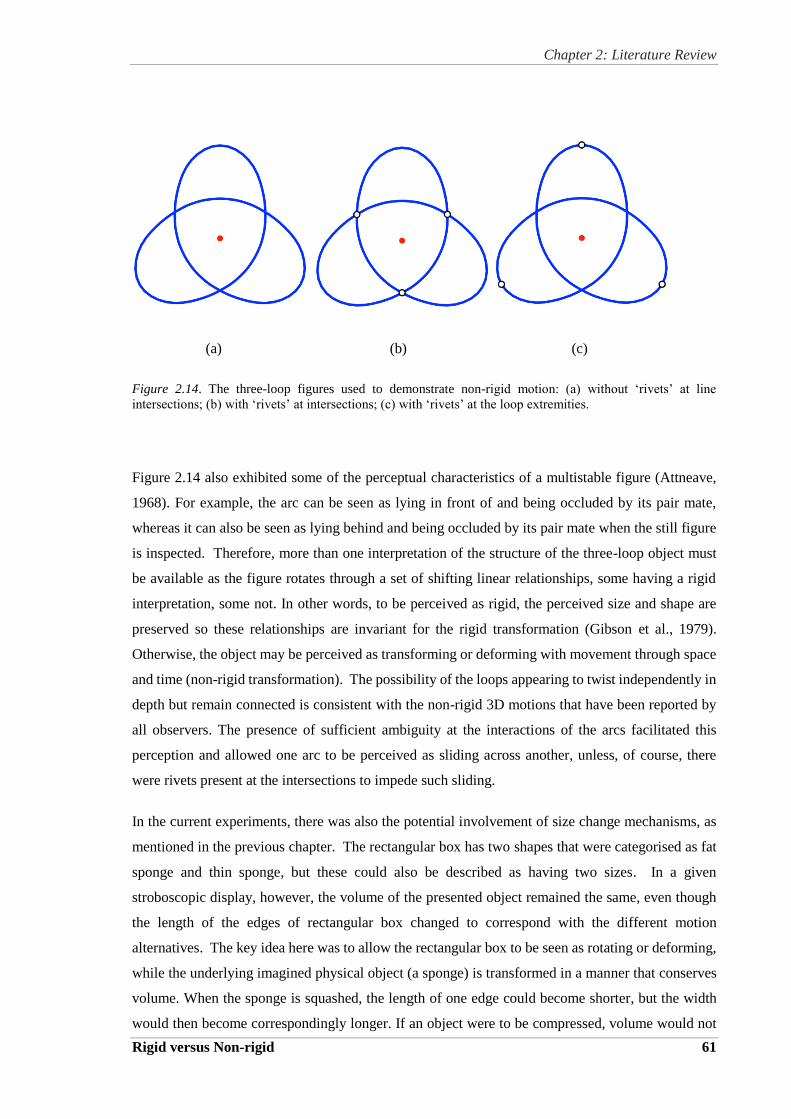
Chapter 2: Literature Review
Rigid versus Non-rigid 61
(a) (b) (c)
Figure 2.14. The three-loop figures used to demonstrate non-rigid motion: (a) without ‘rivets’ at line
intersections; (b) with ‘rivets’ at intersections; (c) with ‘rivets’ at the loop extremities.
Figure 2.14 also exhibited some of the perceptual characteristics of a multistable figure (Attneave,
1968). For example, the arc can be seen as lying in front of and being occluded by its pair mate,
whereas it can also be seen as lying behind and being occluded by its pair mate when the still figure
is inspected. Therefore, more than one interpretation of the structure of the three-loop object must
be available as the figure rotates through a set of shifting linear relationships, some having a rigid
interpretation, some not. In other words, to be perceived as rigid, the perceived size and shape are
preserved so these relationships are invariant for the rigid transformation (Gibson et al., 1979).
Otherwise, the object may be perceived as transforming or deforming with movement through space
and time (non-rigid transformation). The possibility of the loops appearing to twist independently in
depth but remain connected is consistent with the non-rigid 3D motions that have been reported by
all observers. The presence of sufficient ambiguity at the interactions of the arcs facilitated this
perception and allowed one arc to be perceived as sliding across another, unless, of course, there
were rivets present at the intersections to impede such sliding.
In the current experiments, there was also the potential involvement of size change mechanisms, as
mentioned in the previous chapter. The rectangular box has two shapes that were categorised as fat
sponge and thin sponge, but these could also be described as having two sizes. In a given
stroboscopic display, however, the volume of the presented object remained the same, even though
the length of the edges of rectangular box changed to correspond with the different motion
alternatives. The key idea here was to allow the rectangular box to be seen as rotating or deforming,
while the underlying imagined physical object (a sponge) is transformed in a manner that conserves
volume. When the sponge is squashed, the length of one edge could become shorter, but the width
would then become correspondingly longer. If an object were to be compressed, volume would not

Chapter 2: Literature Review
Rigid versus Non-rigid 62
be conserved, and this would not be regarded as minimum change. If the visual system operates
according to several competing principles, one of which is minimum change, other factors that
modulate the resulting motion percepts may come into play, such as shifting surface colours that are
either consistent or incongruent with each of the two percepts. This is precisely the conflict that is
examined in the first experiment reported in this thesis.
Chapter 3: Research Methods
Rigid versus Non-rigid 63
CHAPTER 3: RESEARCH METHODS
This chapter describes the research methods used in the study. Two experiments were conducted.
The first experiment manipulated the shape and colour of stroboscopically presented objects and
explored how these two factors influenced the reported frequency of perception of two types of
motion: rigid rotation versus non-rigid deformation. The results from Experiment 1 informed the
design of Experiment 2, which further investigated the mechanisms underlying the formation of these
two motion percepts. It used an adaptation after-effect in which four different adapting stimuli were
employed.
3.1 Methods Common to the Two Experiments
Both experiments used stroboscopically displayed rectangular boxes to create percepts of visual
motion. Each reported on two competing percepts and examined the mechanisms underlying the
reported motion. In both experiments, the observers were asked to report whether they perceived
rigid rotation or non-rigid deformation; that is, they reported what they saw. These perceptions were
then compared with the actual corresponding stimulus that had been presented. Changes in the
stimulus as the result of changes in the perception were also examined.
Experiment 1 consisted solely of the reporting of the two percepts over a period of time. The
experiment was designed to assess what the observer perceived. The data collected indicated the
proportion of time spent in one state of the multi-stable percept. Experiment 1 used only one of two
tasks, but this was sufficient to demonstrate which of the two percepts observers reported, as well as
the duration. The results made it possible to predict which motion adaptation would be perceived so
that the task could be used again in Experiment 2 (although this was not the main purpose of
Experiment 2).
3.2 Methodological Differences between the Two Experiments
Experiment 1 emphasised colours and shapes. There were three different shapes of rectangular box.
One surface was green and the others were yellow. The green surface was shifted to different
positions in Experiment 1 but was eliminated from Experiment 2, in which only yellow was used.
Chapter 3: Research Methods
Rigid versus Non-rigid 64
Three sizes of rectangular box were used in the control-condition test session, which was conducted
first to identify the most suitable size for Experiment 2. The results of the control-condition test
provided baseline measurements. These were used to assess the effects of motion adaptation on
perceptions of rigid rotation or non-rigid deformation.
Experiment 2 consisted of alternating phases of adaptation and testing. In Phase 1 (adaptation), the
stimulus is shown for a longer period. In Phase 2 (testing), the stimulus is only shown for a very brief
time. The second experiment began with the tasks used in Experiment 1 as adaptation phase, then
the observers made judgements of rigid rotation or non-rigid deformation movement for test displays
interspersed with periods of motion adaptation. The control condition was used as a baseline so
observers were only given the stimuli that provided for adaptation to motion in the adaptation phase
and not for the control condition. Experiment 2 had a higher degree of complexity than Experiment
1 because a different reporting method was used (see below). However the method of Experiment 1
was used during the presentation of the adapting stimuli for the first phase of Experiment 2. In
Experiment 2 it was important to make sure that observers were focused on watching the stimulus
during the adaptation period and that the percepts they were experiencing were monitored.
Experiment 2 provided data about the amount of time during which either of the two percepts was
observed when the adapting stimuli were presented. It was important to ensure that the observers
were watching the stimulus during the adaptation phase in order to be certain that they would
experience the adaptation after-effect that came from watching the stimulus. If this had not been
done, it would have been difficult to show that they were focusing on the screen because they were
actively and continuously engaged in watching and reporting which percept they were experiencing
during the adaptation. To determine if observers saw the after-effects, the testing phase task was
changed. The initial task concerned which of the two percepts was experienced over time. The change
involved asking observers to make instantaneous choices after a brief presentation of the test
stimulus. Several brief presentations were displayed, after which the observers had to choose between
two alternatives. Thus the second task did not involve a continuous report but an instantaneous
categorical choice. This method of eliciting perceptions that result from specific stimuli is known as
probing for the after-effect (Fox and Barton, 2007). Probing for the after-effect was used to ascertain
what percept was experienced at a particular point in time. This was quite different from the task
required in the adapting stimulus presentation, which involved continuous monitoring of which
percept was present. This difference made it a more complex task.
Chapter 3: Research Methods
Rigid versus Non-rigid 65
The experiments had two main purposes: to ensure that people were watching during the adaptation
period and to ascertain what they perceived during the adaptation. Clearly, what observers perceived
during the test phase was an important determinant of what they reported. It was important to clarify
what they perceived during the adaptation and if that influenced what they reported during the test
phase. In other words, it was important to know that they reported what they perceived. This method
was used exclusively in Experiment 1, and no other tasks were involved.
3.3 Methods
3.3.1 Observers
In this study, subjects or participants are referred to as observers. Convenience sampling was used to
recruit observers from friends of the researcher, students and staff in the Faculty of Architecture,
Design and Planning at the University of Sydney.
The study comprised two experiments. In Experiment 1, all observers were volunteers who received
no remuneration. In Experiment 2, observers were offered a gift voucher from Coles or Woolworths
in appreciation of their participation. Although observers ranged from 20 to 65 years of age, the
majority of observers in both experiments were aged between 22 and 46 years. Six observers in
Experiment 1 also participated in Experiment 2. The use of inter-observer correlation was also
performed in a preliminary analysis for finding outlying observers, whose initial results indicated
that their responses were far from the norm established by the large group of observers who
participated in the current study.
A Participation Information Statement (Appendix 8.1) was given to all volunteers before the
experiment was conducted. Those who agreed to participate were asked to complete a Participant
Information Form (Appendix 8.2) on which they indicated that they had normal or corrected-to-
normal vision. Most observers had no previous experience or training in graphic design or video
game design, nor had they received any spatial ability training in the past.
3.3.2 Design
The study was designed to determine which stimulus parameters influence an observer’s perception
of two types of motion possible for a given animated object. As previously explained, observers were
asked to distinguish between two types of motion: rigid rotation and non-rigid deformation. While
different stimuli animations were being played, observers were asked to press specified keys
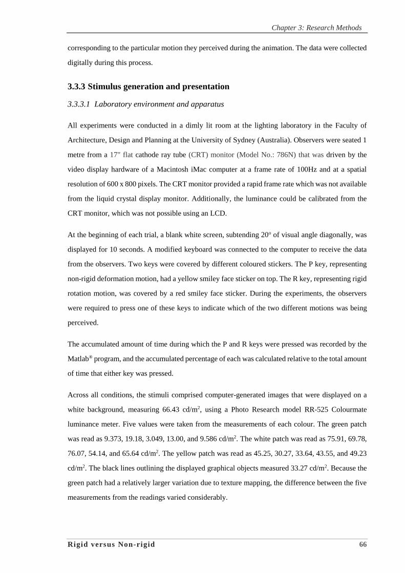
Chapter 3: Research Methods
Rigid versus Non-rigid 66
corresponding to the particular motion they perceived during the animation. The data were collected
digitally during this process.
3.3.3 Stimulus generation and presentation
3.3.3.1 Laboratory environment and apparatus
All experiments were conducted in a dimly lit room at the lighting laboratory in the Faculty of
Architecture, Design and Planning at the University of Sydney (Australia). Observers were seated 1
metre from a 17" flat cathode ray tube (CRT) monitor (Model No.: 786N) that was driven by the
video display hardware of a Macintosh iMac computer at a frame rate of 100Hz and at a spatial
resolution of 600 x 800 pixels. The CRT monitor provided a rapid frame rate which was not available
from the liquid crystal display monitor. Additionally, the luminance could be calibrated from the
CRT monitor, which was not possible using an LCD.
At the beginning of each trial, a blank white screen, subtending 20o of visual angle diagonally, was
displayed for 10 seconds. A modified keyboard was connected to the computer to receive the data
from the observers. Two keys were covered by different coloured stickers. The P key, representing
non-rigid deformation motion, had a yellow smiley face sticker on top. The R key, representing rigid
rotation motion, was covered by a red smiley face sticker. During the experiments, the observers
were required to press one of these keys to indicate which of the two different motions was being
perceived.
The accumulated amount of time during which the P and R keys were pressed was recorded by the
Matlab® program, and the accumulated percentage of each was calculated relative to the total amount
of time that either key was pressed.
Across all conditions, the stimuli comprised computer-generated images that were displayed on a
white background, measuring 66.43 cd/m2, using a Photo Research model RR-525 Colourmate
luminance meter. Five values were taken from the measurements of each colour. The green patch
was read as 9.373, 19.18, 3.049, 13.00, and 9.586 cd/m2. The white patch was read as 75.91, 69.78,
76.07, 54.14, and 65.64 cd/m2. The yellow patch was read as 45.25, 30.27, 33.64, 43.55, and 49.23
cd/m2. The black lines outlining the displayed graphical objects measured 33.27 cd/m2. Because the
green patch had a relatively larger variation due to texture mapping, the difference between the five
measurements from the readings varied considerably.
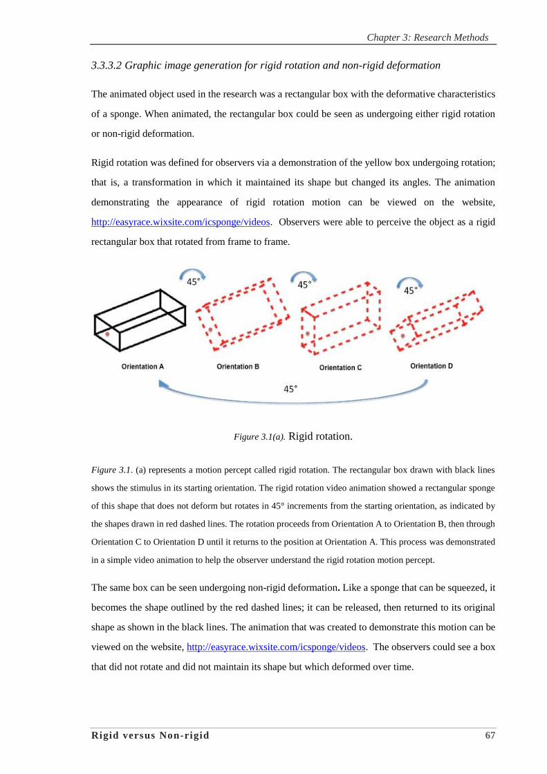
Chapter 3: Research Methods
Rigid versus Non-rigid 67
3.3.3.2 Graphic image generation for rigid rotation and non-rigid deformation
The animated object used in the research was a rectangular box with the deformative characteristics
of a sponge. When animated, the rectangular box could be seen as undergoing either rigid rotation
or non-rigid deformation.
Rigid rotation was defined for observers via a demonstration of the yellow box undergoing rotation;
that is, a transformation in which it maintained its shape but changed its angles. The animation
demonstrating the appearance of rigid rotation motion can be viewed on the website,
http://easyrace.wixsite.com/icsponge/videos. Observers were able to perceive the object as a rigid
rectangular box that rotated from frame to frame.
Figure 3.1(a). Rigid rotation.
Figure 3.1. (a) represents a motion percept called rigid rotation. The rectangular box drawn with black lines
shows the stimulus in its starting orientation. The rigid rotation video animation showed a rectangular sponge
of this shape that does not deform but rotates in 45° increments from the starting orientation, as indicated by
the shapes drawn in red dashed lines. The rotation proceeds from Orientation A to Orientation B, then through
Orientation C to Orientation D until it returns to the position at Orientation A. This process was demonstrated
in a simple video animation to help the observer understand the rigid rotation motion percept.
The same box can be seen undergoing non-rigid deformation. Like a sponge that can be squeezed, it
becomes the shape outlined by the red dashed lines; it can be released, then returned to its original
shape as shown in the black lines. The animation that was created to demonstrate this motion can be
viewed on the website, http://easyrace.wixsite.com/icsponge/videos. The observers could see a box
that did not rotate and did not maintain its shape but which deformed over time.
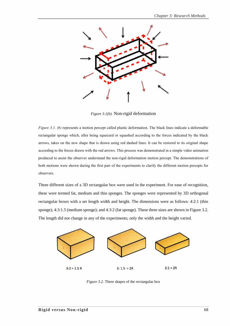
Chapter 3: Research Methods
Rigid versus Non-rigid 68
Figure 3.1(b). Non-rigid deformation
Figure 3.1. (b) represents a motion percept called plastic deformation. The black lines indicate a deformable
rectangular sponge which, after being squeezed or squashed according to the forces indicated by the black
arrows, takes on the new shape that is drawn using red dashed lines. It can be restored to its original shape
according to the forces drawn with the red arrows. This process was demonstrated in a simple video animation
produced to assist the observer understand the non-rigid deformation motion percept. The demonstrations of
both motions were shown during the first part of the experiments to clarify the different motion percepts for
observers.
Three different sizes of a 3D rectangular box were used in the experiment. For ease of recognition,
these were termed fat, medium and thin sponges. The sponges were represented by 3D orthogonal
rectangular boxes with a set length width and height. The dimensions were as follows: 4:2:1 (thin
sponge); 4:3:1.5 (medium sponge); and 4:3:2 (fat sponge). These three sizes are shown in Figure 3.2.
The length did not change in any of the experiments; only the width and the height varied.
Figure 3.2. Three shapes of the rectangular box
Chapter 3: Research Methods
Rigid versus Non-rigid 69
Observers were given the opportunity to view the three differently sized rectangular boxes during
different sessions of the experiments. Each time, the order in which observers were shown the sizes
was randomised.
3.3.3.3 Cycle duration
The total cycle duration for the animation sequence contained 32 frames; the image durations were
strictly controlled by the video frame rate. The duration of each video frame was 10ms, and this was
controlled by the hardware. Therefore the duration of each image in the animation sequence could
be controlled in increments of 10ms. A CRT was used to display stimuli as the frame rate could be
held at 100 video frames per second, a faster rate than that supported by most LCD-based technology.
The superior temporal resolution of the CRT-based display system allowed for the desired control
over the image duration. The two stimulus images were always of equal duration, but the
interstimulus interval (ISI) varied from 10ms to 160ms. The image that was shown during the ISI
contained a fixation point on an otherwise blank screen. As the total number of frames was always
32, the duration of a single animation cycle was always 320ms, The number of ISI frames was
selected to be either 1, 3, 6, 10 or 16, and could be varied from trial to trial under computer program
control. The duration of each image in frames was calculated as 32 minus the ISI frames, which then
became 31, 29, 26, 22, 16 frames. In the limiting case, therefore, the image duration was equal to the
duration of the ISI, for a 50% duty cycle.
In the case of the longest ISI, the image frame was the shortest. The animation cycle was the cycle
duration, which was equal to 64 because the rate of motion was held constant. The number of frames
in one cycle was always 64, but the ISI increased from 1 to 16 frames. As a check, the animation
cycle rate also could be calculated by dividing the total number of cycles presented (which was 94
cycles) by the total duration for the presentation of those cycles (which was 60 seconds). Therefore,
the animation cycle rate was 94/60, or 1.566 cycles/second.
The duty cycle was calculated for the amount of time the object images were shown relative to the
blank image containing only the fixation point. The total period of the sequence was divided by the
percentage of the time during which the image was displayed. In relation to the animation cycle
duration, the blank image containing the fixation point as ISI appears twice, so the ISI has to be
doubled. Therefore the duty cycle could be calculated from animation cycle duration in milliseconds
minus the doubled ISI variable in milliseconds. Finally, the animation cycle duration in milliseconds
was multiplied by 100 to obtain the percentage value. The value of ISI varied from 10ms, 30ms,

Chapter 3: Research Methods
Rigid versus Non-rigid 70
60ms, 100ms to 160ms at different trials. The animation cycle duration remained constant and the
value was always 640ms.
3.4 Procedure
On arrival, observers were given two forms to complete: a Participant Consent Form (Appendix 8.3)
and a Participant Information Form (Appendix 8.1). To save time, some observers had previously
received these forms via email.
After the two forms were filled out, the experiments began. All observers were given an Instruction
Sheet (Appendix 8.4) which explained the two motion perceptions of rigid rotation and non-rigid
deformation as shown in Figures 3.1(a) and 3.1(b) above. After observers had read the Instruction
Sheet, they were shown two videos which provided further clarification of the two motion processes.
Since attention has been shown to be a factor in how the Necker cubes are perceived, participants
were shown the following two Necker cubes displayed in Figures 3.2(a) and 3.2(b). If the observers
focused on the orange circle on the left of Figure 3.2(a), the orange framed square (with the light
orange face) was easier to see as the front face of the cube. If, however, the observer focused on the
blue circle on the right of Figure 3.2(b), the blue framed square (with the light blue face) was more
likely to be seen as the front.
Figure 3.3(a). Focus on orange circle. Figure 3.3(b). Focus on blue circle.
Importantly, the point of visual fixation could influence the reversal of an otherwise identical graphic.
As well, even if the visual stimulus itself does not change over time, the perception that is
experienced by the observers may switch between two alternatives, just as the static presentation of
the Necker cube did in the first part of the instructions they received. The perception of shapes
changing as the result of a change in focus of attention is called the Ternus effect. Although the
appearance of the Necker cube alternates without any attention or conscious effort (due to
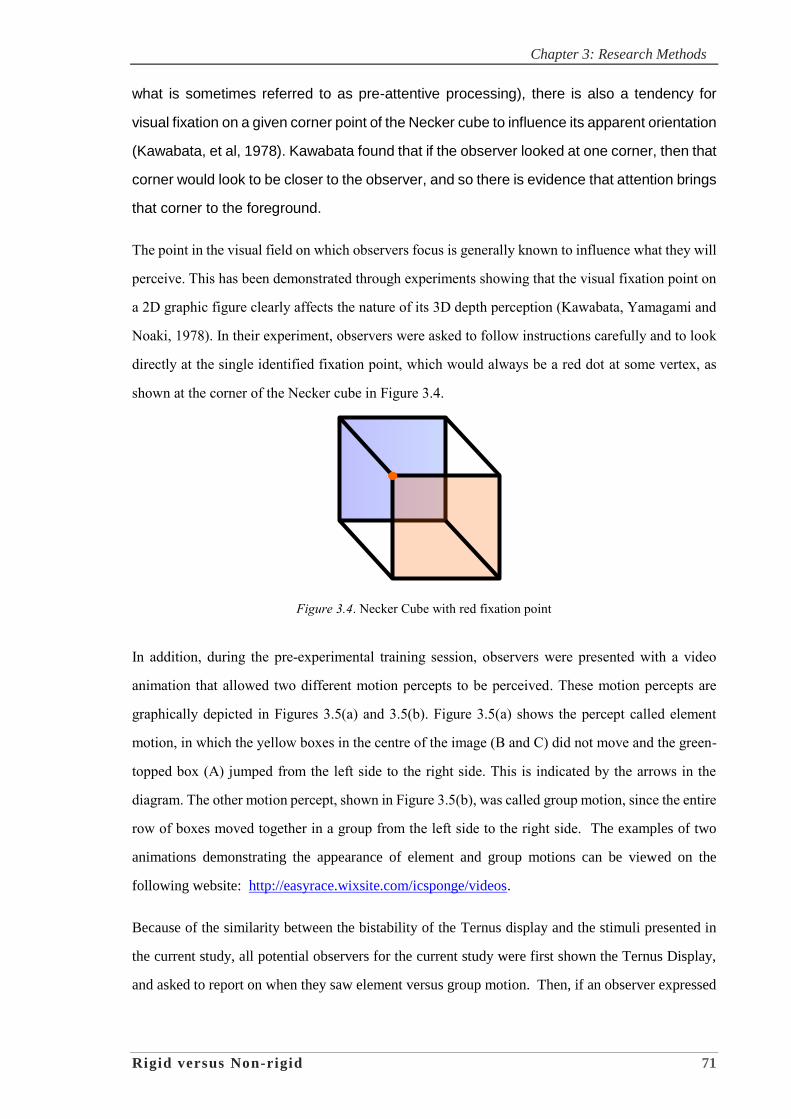
Chapter 3: Research Methods
Rigid versus Non-rigid 71
what is sometimes referred to as pre-attentive processing), there is also a tendency for
visual fixation on a given corner point of the Necker cube to influence its apparent orientation
(Kawabata, et al, 1978). Kawabata found that if the observer looked at one corner, then that
corner would look to be closer to the observer, and so there is evidence that attention brings
that corner to the foreground.
The point in the visual field on which observers focus is generally known to influence what they will
perceive. This has been demonstrated through experiments showing that the visual fixation point on
a 2D graphic figure clearly affects the nature of its 3D depth perception (Kawabata, Yamagami and
Noaki, 1978). In their experiment, observers were asked to follow instructions carefully and to look
directly at the single identified fixation point, which would always be a red dot at some vertex, as
shown at the corner of the Necker cube in Figure 3.4.
Figure 3.4. Necker Cube with red fixation point
In addition, during the pre-experimental training session, observers were presented with a video
animation that allowed two different motion percepts to be perceived. These motion percepts are
graphically depicted in Figures 3.5(a) and 3.5(b). Figure 3.5(a) shows the percept called element
motion, in which the yellow boxes in the centre of the image (B and C) did not move and the green-
topped box (A) jumped from the left side to the right side. This is indicated by the arrows in the
diagram. The other motion percept, shown in Figure 3.5(b), was called group motion, since the entire
row of boxes moved together in a group from the left side to the right side. The examples of two
animations demonstrating the appearance of element and group motions can be viewed on the
following website: http://easyrace.wixsite.com/icsponge/videos.
Because of the similarity between the bistability of the Ternus display and the stimuli presented in
the current study, all potential observers for the current study were first shown the Ternus Display,
and asked to report on when they saw element versus group motion. Then, if an observer expressed
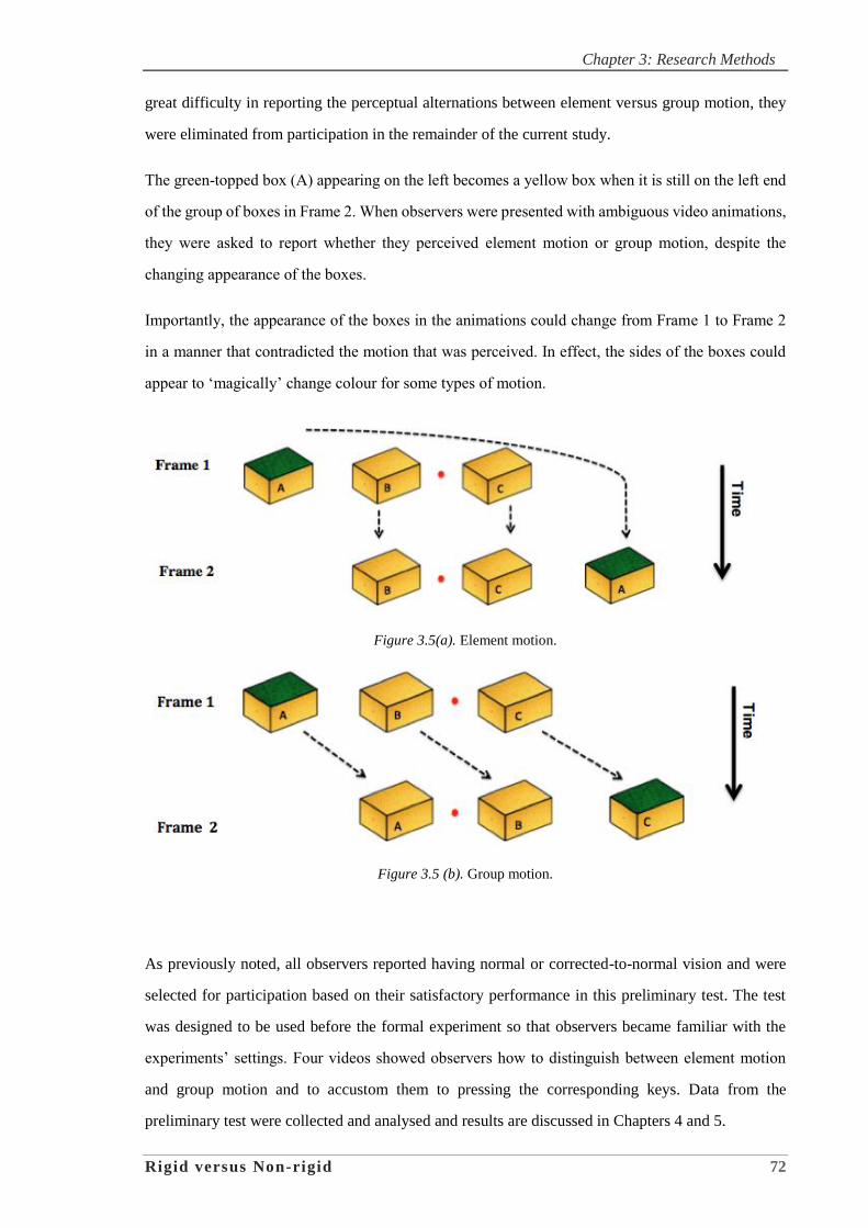
Chapter 3: Research Methods
Rigid versus Non-rigid 72
great difficulty in reporting the perceptual alternations between element versus group motion, they
were eliminated from participation in the remainder of the current study.
The green-topped box (A) appearing on the left becomes a yellow box when it is still on the left end
of the group of boxes in Frame 2. When observers were presented with ambiguous video animations,
they were asked to report whether they perceived element motion or group motion, despite the
changing appearance of the boxes.
Importantly, the appearance of the boxes in the animations could change from Frame 1 to Frame 2
in a manner that contradicted the motion that was perceived. In effect, the sides of the boxes could
appear to ‘magically’ change colour for some types of motion.
Figure 3.5(a). Element motion.
Figure 3.5 (b). Group motion.
As previously noted, all observers reported having normal or corrected-to-normal vision and were
selected for participation based on their satisfactory performance in this preliminary test. The test
was designed to be used before the formal experiment so that observers became familiar with the
experiments’ settings. Four videos showed observers how to distinguish between element motion
and group motion and to accustom them to pressing the corresponding keys. Data from the
preliminary test were collected and analysed and results are discussed in Chapters 4 and 5.
Chapter 3: Research Methods
Rigid versus Non-rigid 73
All observers participated in a practice session to ensure that they could proceed to the formal
experiments with a clear understanding of the instructions. The experiments themselves did not begin
until observers were confident they could follow the instructions. Before proceeding to the
experimental trials, observers were also instructed that they would only be asked to report on what
they PERCEIVED, rather than on what they thought was DISPLAYED. This was intended to direct
their attention to perceptual differences between stimuli, rather than to ideas they had about the
physical stimuli being displayed.
The third part of the procedure was the formal experiment. Observers were presented with a video
that showed the sponge animations that could be perceived undergoing the two different types of
motion. While viewing the sponge animations, observers were reminded to report only what was
PERCEIVED, not what was DISPLAYED (important because some observers wanted to describe
what they thought were the physical parameters of the stimuli).
The formal task for observers during the experiments was to press certain keys according to the
motions they perceived. Observers were given the Instruction Sheet (Appendix 8.4) which explained
that they should press a specific key every time they perceived one of two types of motion percept,
and a different specific key when they saw the other motion percept. The keyboard-pressing activities
were recorded using the Matlab® program when observers pressed and released the buttons. When
they perceived a change in motion from one type to another, they were instructed to switch between
keys to indicate the change. The key with the yellow smiley face represented P for non-rigid
deformation motion and the key with the red smiley face represented R for rigid rotation. The
program recorded the exact time at which the keys were pressed. Observers were asked to press the
key with the red smiley face on the left side of the keyboard until they encountered the other motion
(i.e. non-rigid deformation), at which time they were to release the current button before switching
to the other one (to indicate that they were perceiving rigid rotation).
Throughout the experiment, only the red smiley face and yellow smiley face keys were to be pressed;
the program did not record any other key presses. If another key was pressed, the program generated
an error. Observers could elect to take breaks during the experiment if they experienced fatigue.
After the observers had completed all sessions they were given an Evaluation Form (Appendix 8.5).
The form contained four questions about their reflections on the experiment.

Chapter 3: Research Methods
Rigid versus Non-rigid 74
3.5 Recording Methods and Results Calculations
When observers pressed the respective response keys, several values were recorded in the Matlab®
files. When the red smiley face key was pressed, this indicated that rigid rotation motion was
perceived. The response R value was stored in the Matlab® file and the precise ‘pressed time’ of rigid
rotation was recorded. When the observer released the key, the ‘released time’ of non-rigid
deformation was recorded in the Matlab® file.
When the yellow smiley face key was pressed, this indicated that non-rigid deformation motion was
perceived. The response P value was stored in the Matlab® file and the precise moment the key was
pressed was stored in the Matlab® file as the ‘pressed time’ of non-rigid deformation. When the
observer released the key, the response ‘released time’ of non-rigid deformation was recorded.
The number of P and R responses was accumulated and stored in the Matlab® file. The duration of
time between pressing and release of the two keys was calculated by ‘released time’ minus ‘pressed
time’ using a program file that automatically generated the values. The results were stored in a
Matlab® file. Once the duration of each key press had been calculated, the temporal response
proportion was calculated using the following simple equation:
temporal response ‘R’ proportion =temporal response ‘R’ duration
temporal response ‘R’ duration + temporal response ‘P’ duration
Hence, three values were obtained from calculation of the raw data:
1. The duration in milliseconds of the rigid rotation and non-rigid deformation of each key
pressed
2. The temporal response R proportion from each experiment
3. The raw proportion of the number of times rigid rotation and non-rigid deformation was
recorded through key presses from each of the experimental sessions.
From these values, a histogram was plotted to summarise the duration and key presses according to
the observed distribution. The results are presented in Chapters 4 and 5.
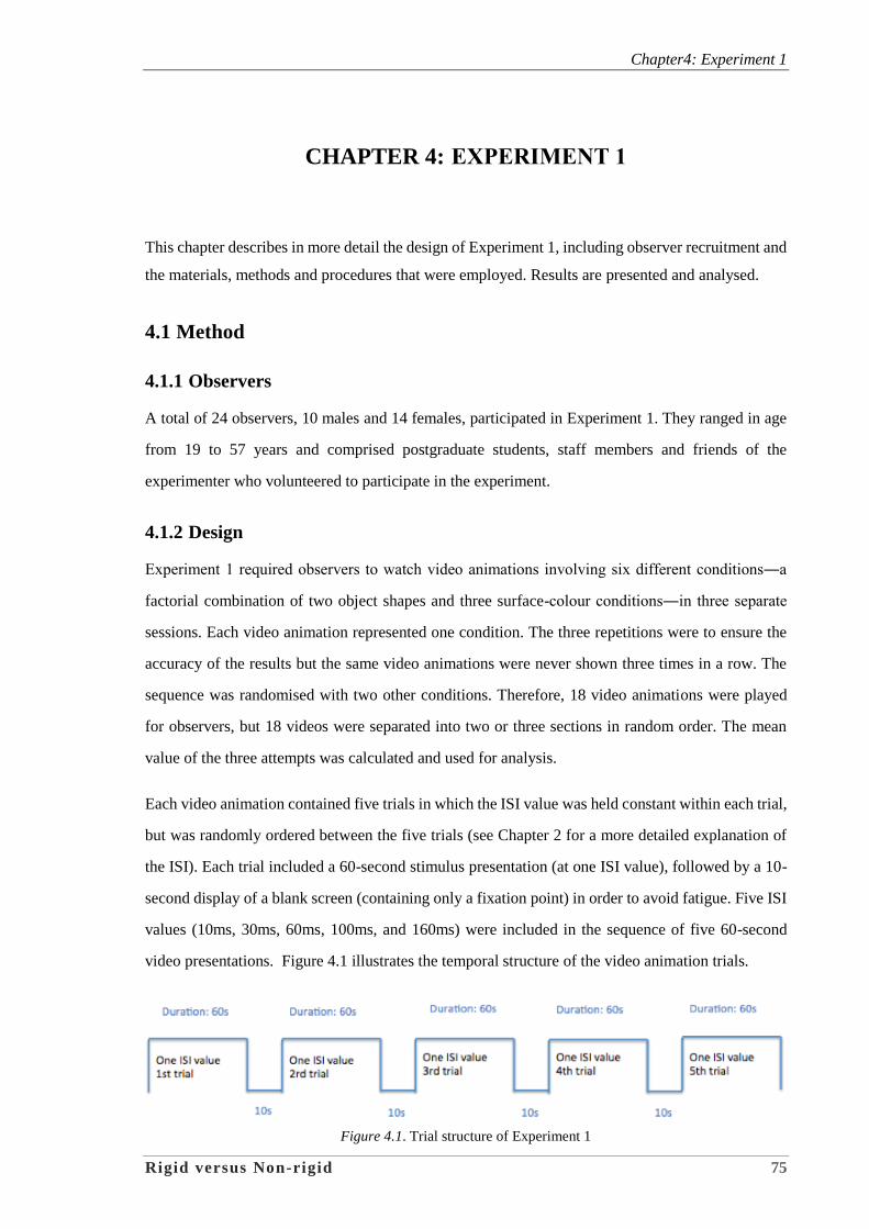
Chapter4: Experiment 1
Rigid versus Non-rigid 75
CHAPTER 4: EXPERIMENT 1
This chapter describes in more detail the design of Experiment 1, including observer recruitment and
the materials, methods and procedures that were employed. Results are presented and analysed.
4.1 Method
4.1.1 Observers
A total of 24 observers, 10 males and 14 females, participated in Experiment 1. They ranged in age
from 19 to 57 years and comprised postgraduate students, staff members and friends of the
experimenter who volunteered to participate in the experiment.
4.1.2 Design
Experiment 1 required observers to watch video animations involving six different conditions―a
factorial combination of two object shapes and three surface-colour conditions―in three separate
sessions. Each video animation represented one condition. The three repetitions were to ensure the
accuracy of the results but the same video animations were never shown three times in a row. The
sequence was randomised with two other conditions. Therefore, 18 video animations were played
for observers, but 18 videos were separated into two or three sections in random order. The mean
value of the three attempts was calculated and used for analysis.
Each video animation contained five trials in which the ISI value was held constant within each trial,
but was randomly ordered between the five trials (see Chapter 2 for a more detailed explanation of
the ISI). Each trial included a 60-second stimulus presentation (at one ISI value), followed by a 10-
second display of a blank screen (containing only a fixation point) in order to avoid fatigue. Five ISI
values (10ms, 30ms, 60ms, 100ms, and 160ms) were included in the sequence of five 60-second
video presentations. Figure 4.1 illustrates the temporal structure of the video animation trials.
Figure 4.1. Trial structure of Experiment 1

Chapter4: Experiment 1
Rigid versus Non-rigid 76
The videos shown in each trial consisted of a sequence of three different images that were shown in
the following order: Image 1, Fixation ISI Image (with fixation point only), Image 2, Fixation ISI
Image (with fixation point only), Image 1 (to start the sequence again). Note that, for a given object
shape (thin or fat), the object could be either all yellow or could have a single green face.
Furthermore, that green face could either shift spatially in a manner consistent with rigid rotation, or
could remain spatially stationary on the top side of the object, in a manner consistent with non-rigid
deformation.
Before beginning experimental trials, participants were presented with two videos that were designed
to clearly demonstrate the two types of motion likely to be perceived when viewing the bistable
stroboscopic stimuli, as was discussed in Chapter 3. That is, these videos demonstrated an
unambiguous display of rigid rotation and non-rigid deformation. Images 1 and 2 for the two different
images were each presented for a fixed number of video frames at the CRT frame rate of 100ms. An
example sequence from one of the conditions is illustrated in Figure 4.2.(a), in which Image 1 is
Image 1GT representing the thin sponge with a green top (i.e. green top facing upwards), Image 2 is
Image 2GT representing the thin sponge with a green side (i.e. green side facing upwards). As
mentioned previously, a factorial combination of the surface-colour and two object shapes was being
tested in Experiment 1; in between is a white screen containing only the fixation point (labelled
“Fixation ISI”).
Figure 4.2.(a) Green-stationary thin
Similarly, in Figure 4.2.(b), Image 1 is Image 1GF representing the fat sponge with a green top (i.e.
green top facing upwards) and Image 2 is Image 2GF representing the fat sponge with a green side
(i.e. green side still facing upwards).
Image 2GT: ISI x 10ms
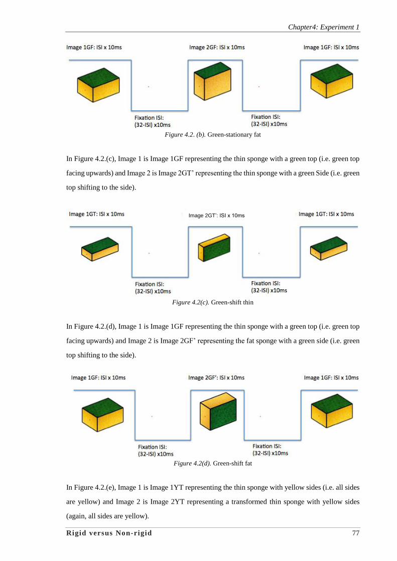
Chapter4: Experiment 1
Rigid versus Non-rigid 77
Figure 4.2. (b). Green-stationary fat
In Figure 4.2.(c), Image 1 is Image 1GF representing the thin sponge with a green top (i.e. green top
facing upwards) and Image 2 is Image 2GT’ representing the thin sponge with a green Side (i.e. green
top shifting to the side).
Figure 4.2(c). Green-shift thin
In Figure 4.2.(d), Image 1 is Image 1GF representing the thin sponge with a green top (i.e. green top
facing upwards) and Image 2 is Image 2GF’ representing the fat sponge with a green side (i.e. green
top shifting to the side).
Figure 4.2(d). Green-shift fat
In Figure 4.2.(e), Image 1 is Image 1YT representing the thin sponge with yellow sides (i.e. all sides
are yellow) and Image 2 is Image 2YT representing a transformed thin sponge with yellow sides
(again, all sides are yellow).
Image 2GT’: ISI x 10ms
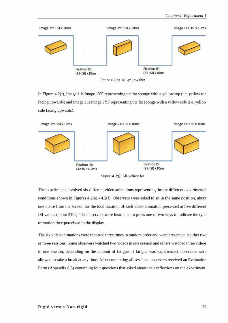
Chapter4: Experiment 1
Rigid versus Non-rigid 78
Figure 4.2(e). All-yellow thin
In Figure 4.2(f), Image 1 is Image 1YF representing the fat sponge with a yellow top (i.e. yellow top
facing upwards) and Image 2 is Image 2YF representing the fat sponge with a yellow side (i.e. yellow
side facing upwards).
Figure 4.2(f). All-yellow fat
The experiments involved six different video animations representing the six different experimental
conditions shown in Figures 4.2(a) - 4.2(f). Observers were asked to sit in the same position, about
one metre from the screen, for the total duration of each video animation presented at five different
ISI values (about 340s). The observers were instructed to press one of two keys to indicate the type
of motion they perceived in the display.
The six video animations were repeated three times in random order and were presented in either two
or three sessions. Some observers watched two videos in one session and others watched three videos
in one session, depending on the amount of fatigue. If fatigue was experienced, observers were
allowed to take a break at any time. After completing all sessions, observers received an Evaluation
Form (Appendix 8.5) containing four questions that asked about their reflections on the experiment.
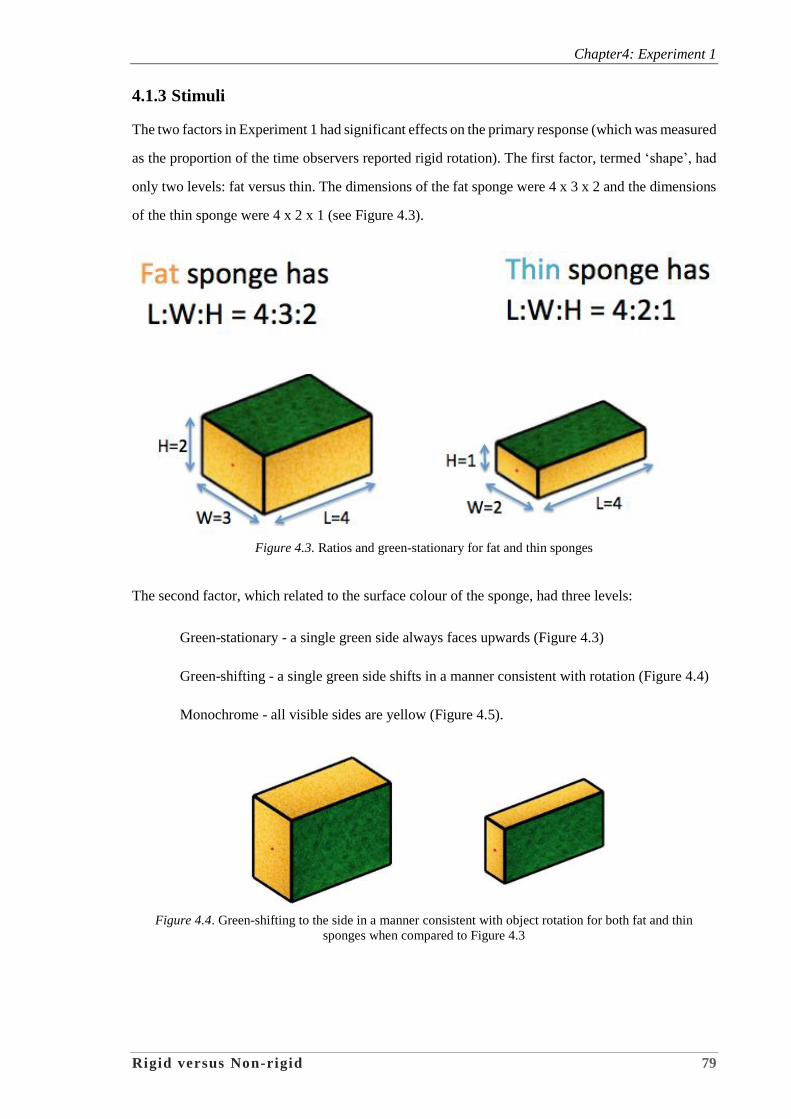
Chapter4: Experiment 1
Rigid versus Non-rigid 79
4.1.3 Stimuli
The two factors in Experiment 1 had significant effects on the primary response (which was measured
as the proportion of the time observers reported rigid rotation). The first factor, termed ‘shape’, had
only two levels: fat versus thin. The dimensions of the fat sponge were 4 x 3 x 2 and the dimensions
of the thin sponge were 4 x 2 x 1 (see Figure 4.3).
Figure 4.3. Ratios and green-stationary for fat and thin sponges
The second factor, which related to the surface colour of the sponge, had three levels:
Green-stationary - a single green side always faces upwards (Figure 4.3)
Green-shifting - a single green side shifts in a manner consistent with rotation (Figure 4.4)
Monochrome - all visible sides are yellow (Figure 4.5).
Figure 4.4. Green-shifting to the side in a manner consistent with object rotation for both fat and thin
sponges when compared to Figure 4.3
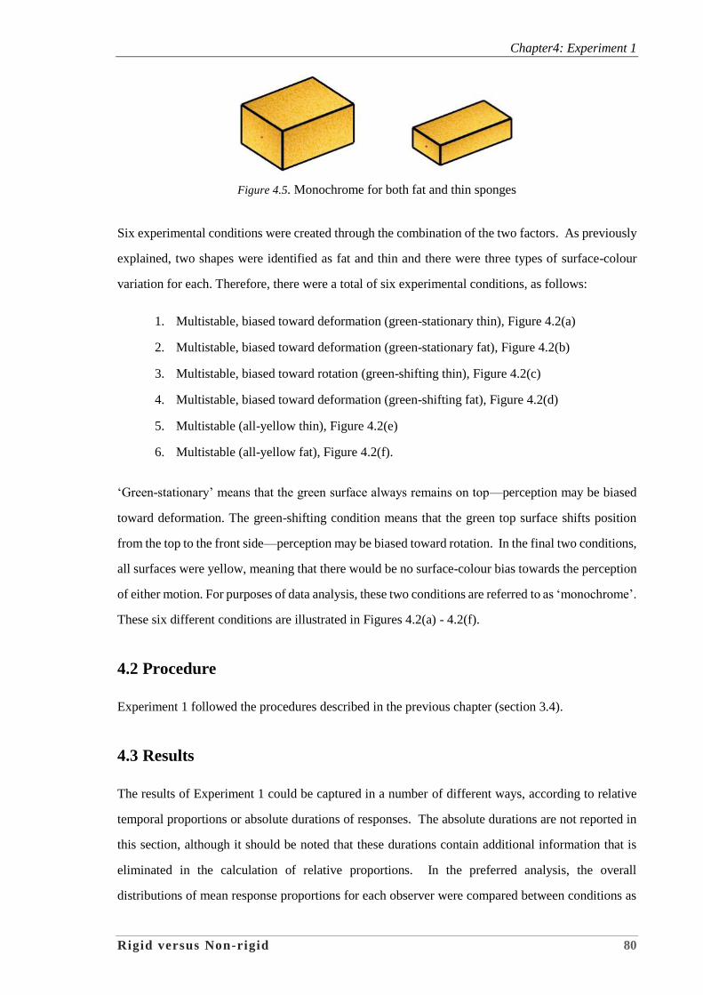
Chapter4: Experiment 1
Rigid versus Non-rigid 80
Figure 4.5. Monochrome for both fat and thin sponges
Six experimental conditions were created through the combination of the two factors. As previously
explained, two shapes were identified as fat and thin and there were three types of surface-colour
variation for each. Therefore, there were a total of six experimental conditions, as follows:
1. Multistable, biased toward deformation (green-stationary thin), Figure 4.2(a)
2. Multistable, biased toward deformation (green-stationary fat), Figure 4.2(b)
3. Multistable, biased toward rotation (green-shifting thin), Figure 4.2(c)
4. Multistable, biased toward deformation (green-shifting fat), Figure 4.2(d)
5. Multistable (all-yellow thin), Figure 4.2(e)
6. Multistable (all-yellow fat), Figure 4.2(f).
‘Green-stationary’ means that the green surface always remains on top—perception may be biased
toward deformation. The green-shifting condition means that the green top surface shifts position
from the top to the front side—perception may be biased toward rotation. In the final two conditions,
all surfaces were yellow, meaning that there would be no surface-colour bias towards the perception
of either motion. For purposes of data analysis, these two conditions are referred to as ‘monochrome’.
These six different conditions are illustrated in Figures 4.2(a) - 4.2(f).
4.2 Procedure
Experiment 1 followed the procedures described in the previous chapter (section 3.4).
4.3 Results
The results of Experiment 1 could be captured in a number of different ways, according to relative
temporal proportions or absolute durations of responses. The absolute durations are not reported in
this section, although it should be noted that these durations contain additional information that is
eliminated in the calculation of relative proportions. In the preferred analysis, the overall
distributions of mean response proportions for each observer were compared between conditions as
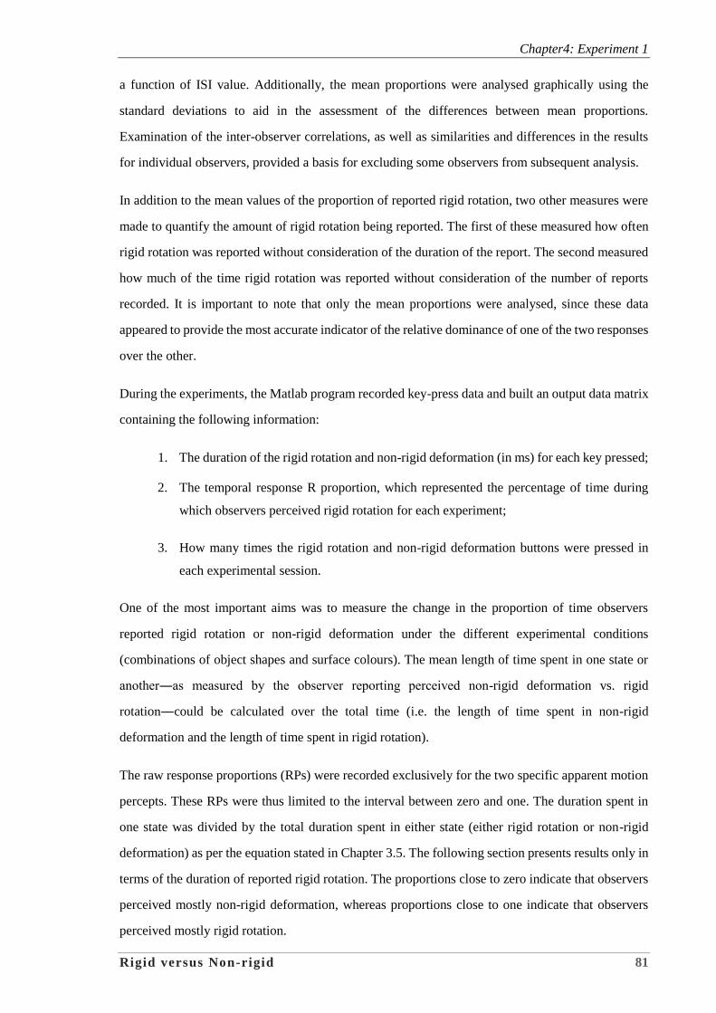
Chapter4: Experiment 1
Rigid versus Non-rigid 81
a function of ISI value. Additionally, the mean proportions were analysed graphically using the
standard deviations to aid in the assessment of the differences between mean proportions.
Examination of the inter-observer correlations, as well as similarities and differences in the results
for individual observers, provided a basis for excluding some observers from subsequent analysis.
In addition to the mean values of the proportion of reported rigid rotation, two other measures were
made to quantify the amount of rigid rotation being reported. The first of these measured how often
rigid rotation was reported without consideration of the duration of the report. The second measured
how much of the time rigid rotation was reported without consideration of the number of reports
recorded. It is important to note that only the mean proportions were analysed, since these data
appeared to provide the most accurate indicator of the relative dominance of one of the two responses
over the other.
During the experiments, the Matlab program recorded key-press data and built an output data matrix
containing the following information:
1. The duration of the rigid rotation and non-rigid deformation (in ms) for each key pressed;
2. The temporal response R proportion, which represented the percentage of time during
which observers perceived rigid rotation for each experiment;
3. How many times the rigid rotation and non-rigid deformation buttons were pressed in
each experimental session.
One of the most important aims was to measure the change in the proportion of time observers
reported rigid rotation or non-rigid deformation under the different experimental conditions
(combinations of object shapes and surface colours). The mean length of time spent in one state or
another―as measured by the observer reporting perceived non-rigid deformation vs. rigid
rotation―could be calculated over the total time (i.e. the length of time spent in non-rigid
deformation and the length of time spent in rigid rotation).
The raw response proportions (RPs) were recorded exclusively for the two specific apparent motion
percepts. These RPs were thus limited to the interval between zero and one. The duration spent in
one state was divided by the total duration spent in either state (either rigid rotation or non-rigid
deformation) as per the equation stated in Chapter 3.5. The following section presents results only in
terms of the duration of reported rigid rotation. The proportions close to zero indicate that observers
perceived mostly non-rigid deformation, whereas proportions close to one indicate that observers
perceived mostly rigid rotation.
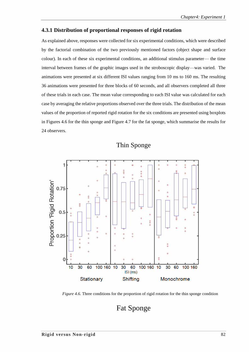
Chapter4: Experiment 1
Rigid versus Non-rigid 82
4.3.1 Distribution of proportional responses of rigid rotation
As explained above, responses were collected for six experimental conditions, which were described
by the factorial combination of the two previously mentioned factors (object shape and surface
colour). In each of these six experimental conditions, an additional stimulus parameter— the time
interval between frames of the graphic images used in the stroboscopic display—was varied. The
animations were presented at six different ISI values ranging from 10 ms to 160 ms. The resulting
36 animations were presented for three blocks of 60 seconds, and all observers completed all three
of these trials in each case. The mean value corresponding to each ISI value was calculated for each
case by averaging the relative proportions observed over the three trials. The distribution of the mean
values of the proportion of reported rigid rotation for the six conditions are presented using boxplots
in Figures 4.6 for the thin sponge and Figure 4.7 for the fat sponge, which summarise the results for
24 observers.
Thin Sponge
Figure 4.6. Three conditions for the proportion of rigid rotation for the thin sponge condition
Fat Sponge
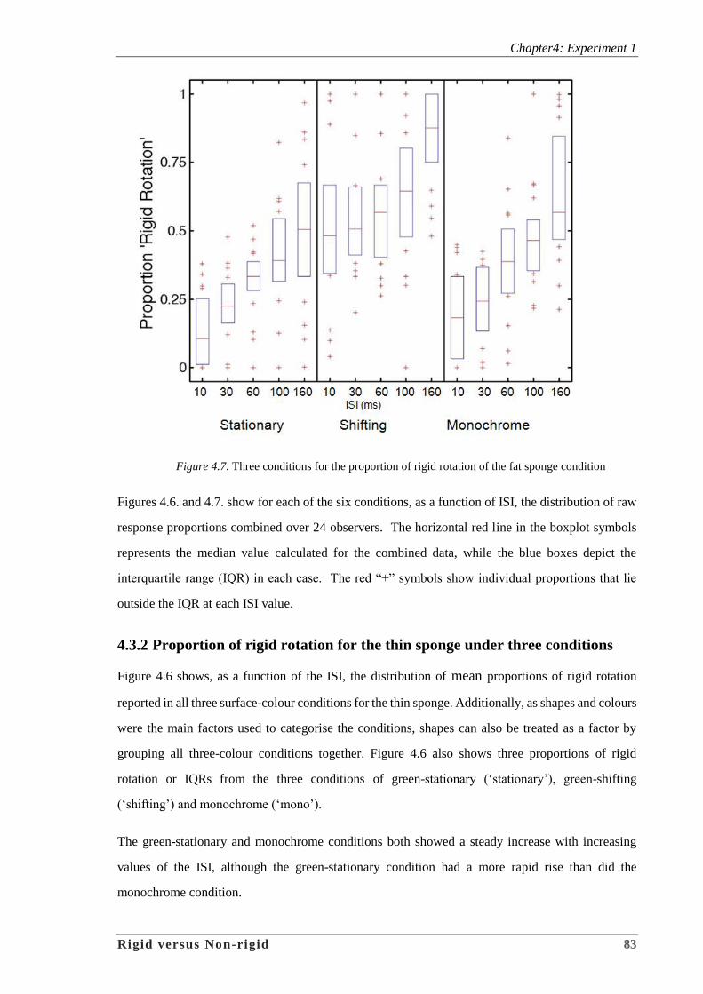
Chapter4: Experiment 1
Rigid versus Non-rigid 83
Figure 4.7. Three conditions for the proportion of rigid rotation of the fat sponge condition
Figures 4.6. and 4.7. show for each of the six conditions, as a function of ISI, the distribution of raw
response proportions combined over 24 observers. The horizontal red line in the boxplot symbols
represents the median value calculated for the combined data, while the blue boxes depict the
interquartile range (IQR) in each case. The red “+” symbols show individual proportions that lie
outside the IQR at each ISI value.
4.3.2 Proportion of rigid rotation for the thin sponge under three conditions
Figure 4.6 shows, as a function of the ISI, the distribution of mean proportions of rigid rotation
reported in all three surface-colour conditions for the thin sponge. Additionally, as shapes and colours
were the main factors used to categorise the conditions, shapes can also be treated as a factor by
grouping all three-colour conditions together. Figure 4.6 also shows three proportions of rigid
rotation or IQRs from the three conditions of green-stationary (‘stationary’), green-shifting
(‘shifting’) and monochrome (‘mono’).
The green-stationary and monochrome conditions both showed a steady increase with increasing
values of the ISI, although the green-stationary condition had a more rapid rise than did the
monochrome condition.

Chapter4: Experiment 1
Rigid versus Non-rigid 84
It is important to note that, in comparison to the other two conditions, green-shifting did not show
the same effect as the ISI values increased. The ISI between 10ms and 60ms for rigid rotation at this
range remained almost the same, but the IQRs displayed a sudden increase in the ISI from 100ms to
160ms. In addition, the median ISI for this condition occurred at 10ms and hovered around 0.62,
which was much higher than for the other two conditions.
4.3.3 Proportion of rigid rotation for the fat sponge under three conditions
Figure 4.7 shows the median proportion of rigid rotation in all three surface-colour conditions for the
fat sponge. A similar pattern can be observed in the fat sponge condition. The conditions of green-
stationary and monochrome showed the same increase in the proportions for rigid rotation for the
different values of ISI. The pattern for the green-shifting condition (middle diagram), however, was
different from that for the other two conditions.
The median value of rigid rotation for the lower value of ISI 10ms in the green-shifting condition
was approximately 0.5. This value was much higher than that for the other two conditions, which
were both below 0.25 at the same ISI. When the ISI values were between 10ms and 100ms, the four
medians of rigid rotation were all between 0.5 and 0.62, with a slow increase. The median
corresponding to the ISI at 160ms had the highest value at almost 0.85.
Note that the above results come from the analysis of data from the entire group of 24
observers; however, there were some individual differences that were deemed worthy of
examination, as discussed in detail in the following section.
In summary, when the shapes of thin and fat sponges and the three conditions of surface-colour
were compared, a higher proportion of rigid rotation occurred in relation to green-shifting for both
the thin and fat sponges (Figure 4.6. and Figure 4.7.). Column 2 in both figures shows the highest
median of rigid rotation perception, which was approximately 0.85 when the ISI was at 160 ms. This
means that observers perceived the most rigid rotation motion in the green-shifting condition for both
thin and fat sponges when the ISI was at the highest ISI value presented. Specifically, it seems that
the green-shifting condition promoted a greater likelihood of perceiving rigid rotation motion when
compared to other conditions at other ISI values. The factor of shapes showed little influence when
compared to the factor of surface-colour.
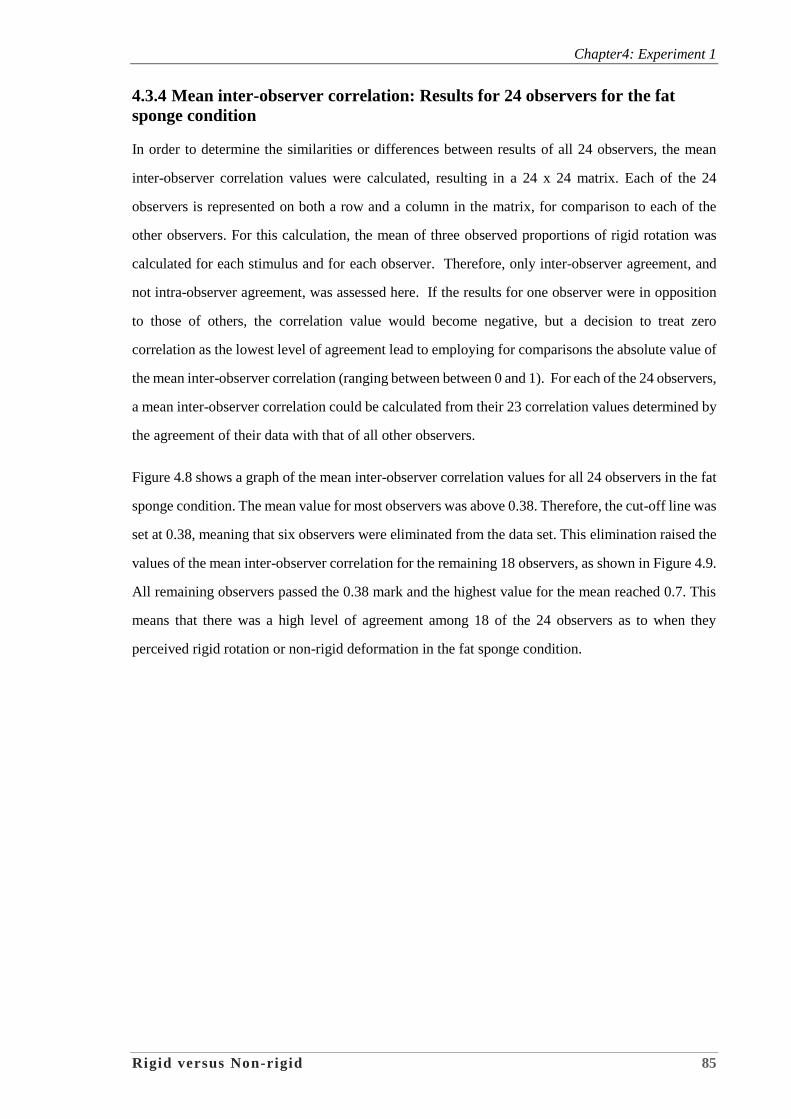
Chapter4: Experiment 1
Rigid versus Non-rigid 85
4.3.4 Mean inter-observer correlation: Results for 24 observers for the fat
sponge condition
In order to determine the similarities or differences between results of all 24 observers, the mean
inter-observer correlation values were calculated, resulting in a 24 x 24 matrix. Each of the 24
observers is represented on both a row and a column in the matrix, for comparison to each of the
other observers. For this calculation, the mean of three observed proportions of rigid rotation was
calculated for each stimulus and for each observer. Therefore, only inter-observer agreement, and
not intra-observer agreement, was assessed here. If the results for one observer were in opposition
to those of others, the correlation value would become negative, but a decision to treat zero
correlation as the lowest level of agreement lead to employing for comparisons the absolute value of
the mean inter-observer correlation (ranging between between 0 and 1). For each of the 24 observers,
a mean inter-observer correlation could be calculated from their 23 correlation values determined by
the agreement of their data with that of all other observers.
Figure 4.8 shows a graph of the mean inter-observer correlation values for all 24 observers in the fat
sponge condition. The mean value for most observers was above 0.38. Therefore, the cut-off line was
set at 0.38, meaning that six observers were eliminated from the data set. This elimination raised the
values of the mean inter-observer correlation for the remaining 18 observers, as shown in Figure 4.9.
All remaining observers passed the 0.38 mark and the highest value for the mean reached 0.7. This
means that there was a high level of agreement among 18 of the 24 observers as to when they
perceived rigid rotation or non-rigid deformation in the fat sponge condition.
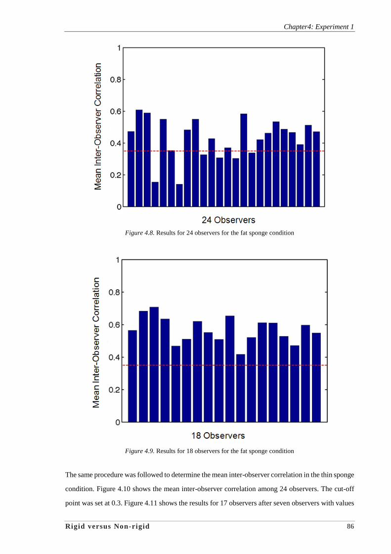
Chapter4: Experiment 1
Rigid versus Non-rigid 86
Figure 4.8. Results for 24 observers for the fat sponge condition
Figure 4.9. Results for 18 observers for the fat sponge condition
The same procedure was followed to determine the mean inter-observer correlation in the thin sponge
condition. Figure 4.10 shows the mean inter-observer correlation among 24 observers. The cut-off
point was set at 0.3. Figure 4.11 shows the results for 17 observers after seven observers with values
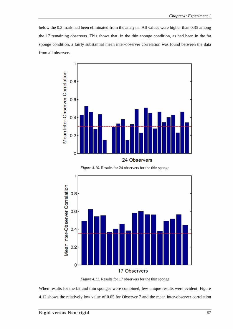
Chapter4: Experiment 1
Rigid versus Non-rigid 87
below the 0.3 mark had been eliminated from the analysis. All values were higher than 0.35 among
the 17 remaining observers. This shows that, in the thin sponge condition, as had been in the fat
sponge condition, a fairly substantial mean inter-observer correlation was found between the data
from all observers.
Figure 4.10. Results for 24 observers for the thin sponge
Figure 4.11. Results for 17 observers for the thin sponge
When results for the fat and thin sponges were combined, few unique results were evident. Figure
4.12 shows the relatively low value of 0.05 for Observer 7 and the mean inter-observer correlation
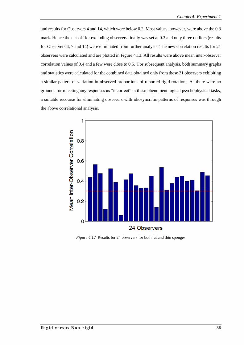
Chapter4: Experiment 1
Rigid versus Non-rigid 88
and results for Observers 4 and 14, which were below 0.2. Most values, however, were above the 0.3
mark. Hence the cut-off for excluding observers finally was set at 0.3 and only three outliers (results
for Observers 4, 7 and 14) were eliminated from further analysis. The new correlation results for 21
observers were calculated and are plotted in Figure 4.13. All results were above mean inter-observer
correlation values of 0.4 and a few were close to 0.6. For subsequent analysis, both summary graphs
and statistics were calculated for the combined data obtained only from these 21 observers exhibiting
a similar pattern of variation in observed proportions of reported rigid rotation. As there were no
grounds for rejecting any responses as “incorrect” in these phenomenological psychophysical tasks,
a suitable recourse for eliminating observers with idiosyncratic patterns of responses was through
the above correlational analysis.
Figure 4.12. Results for 24 observers for both fat and thin sponges
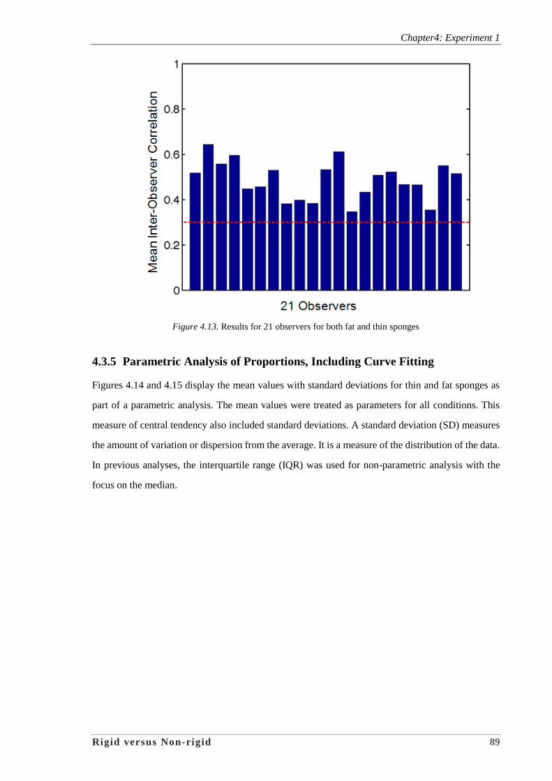
Chapter4: Experiment 1
Rigid versus Non-rigid 89
Figure 4.13. Results for 21 observers for both fat and thin sponges
4.3.5 Parametric Analysis of Proportions, Including Curve Fitting
Figures 4.14 and 4.15 display the mean values with standard deviations for thin and fat sponges as
part of a parametric analysis. The mean values were treated as parameters for all conditions. This
measure of central tendency also included standard deviations. A standard deviation (SD) measures
the amount of variation or dispersion from the average. It is a measure of the distribution of the data.
In previous analyses, the interquartile range (IQR) was used for non-parametric analysis with the
focus on the median.

Chapter4: Experiment 1
Rigid versus Non-rigid 90
Figure 4.14. Thin sponge means with standard deviations
Figure 4.15. Fat sponge means with standard deviations
The downward-facing (magenta) triangles in the figures above represent the mean proportions for
the condition in which the sponge’s green surface always stayed on the top, labelled here as
‘stationary’. The upward-facing (green) triangles represent the mean proportions for the condition in
Chapter4: Experiment 1
Rigid versus Non-rigid 91
which the sponge’s green surface shifted position in different frames (‘shifting’). The yellow circles
represent the mean proportions for the condition in which the sponge’s colour was entirely yellow
(monochrome, abbreviated to ‘mono’). In the figures, the standard deviations of the individual
observer means are indicated by vertical bars.
One notable feature of the data for the thin sponge in Figure 4.14 is that the means for all three
conditions converged at response proportions around 0.75 at 160ms ISI. This common endpoint did
not occur for the fat sponge at 160ms ISI. Although for the fat sponge the response proportions in
the shifting condition also reached 0.75, for the other two conditions (mono and stationary) the mean
values were much lower (reaching only 0.6 and 0.4).
Over all the three conditions, Figure 4.14 shows that the mean response proportion values at 10ms
for the thin sponge were much higher than the mean values for the fat sponge as shown in Figure
4.15. The response proportion value for the shifting condition of the thin sponge at 10ms ISI was
approximately 0.63 but, for the same condition for the fat sponge, it was approximately 0.5. The
value of the mean for the mono condition for the fat sponge was much lower for the thin sponge
under the same condition at 10ms ISI. Finally, the value of the mean for the stationary condition for
the fat sponge started at an extremely low point of 0.1 at 10ms ISI.
The monochrome condition (labelled ‘Mono’ in the legends) could be regarded as a control condition
for comparison to the other two experimental conditions. For the thin object, the shifting surface
colour condition showed a result similar to the control condition in the Figure 4.14. However, the
stationary condition yielded a larger decrease in proportion of rigid rotation reports than the other
two conditions. At all ISI values less than 160 ms, observers clearly perceived much more non-rigid
rotation here. To summarise, the surface colour that was held stationary in a manner consistent with
deformation had a more significant impact in the thin sponge condition than in the thin sponge
condition.
The control condition was compared to the other conditions. For the fat sponge, it seems that the
mean values found in the stationary condition were similar to those of the control condition, but the
mean values were generally higher for the shifting condition. This shows that much more rigid
rotation was perceived for the shifting condition than for the other two conditions. Therefore, the
surface colour that shifted in a manner consistent with rotation had a more significant impact in the
fat sponge condition than in the thin sponge condition.
Chapter4: Experiment 1
Rigid versus Non-rigid 92
One common phenomenon is that both the fat and thin sponge conditions were clearly affected by
the increase of ISI values, since all conditions showed a steady increase from left to right
corresponding to the increase in ISI. This shows that the ISI values had an influence on all the
conditions of the experiments for the mean proportion of rigid rotation reported. Again, it is important
to note that lines have been drawn between corresponding ISI values to aid in identifying trends, but
it will be useful to examine a continuous smooth curve fit to the data collected at ISI values of 10ms,
30ms, 60ms, 100ms and 160ms. However, due to the inherent compression of extreme proportion
values, it was decided to perform the smooth curve fit on Z-transformed data, which would not be
constrained to the interval between zero and one, as the proportion data were.
4.3.6 Z-scores
The previous figures, showing the means and standard deviations of the proportion of rigid rotation
reported as a function of ISI, revealed a high correlation between these variables in all cases.
Nonetheless, it was rather difficult to find the point at which the sets of proportions crossed the 0.5
point, in an effort to identify exact ISI values at which the dominant response shifted from non-rigid
deformation to rigid rotation. Therefore, smooth curves were fit to Z-scores using polynomial
regression analysis. As a special case of multiple linear regression, polynomial regression is a non-
linear transformation that translates data into curves rather than lines to more accurately reflect the
data observed. As the proportions decreased towards zero, the Z-scores became increasingly
negative. As the proportions ascended towards one, the Z-scores continued in a positive direction, in
both cases, with values unconstrained by a fixed limit.
4.3.7 Fat sponge
The mean value of the raw proportions was used to calculate the Z-score. When transformed into a
Z-Score, a non-linear function can be fit to the data, and this is why polynomial regression was used
here. If the Z-score is above 0, observers reported more rigid rotation. If the values are below 0, more
non-rigid deformation was reported. Therefore, the Z-Score is positive when there is more rigid
rotation and negative when there is a higher frequency of non-rigid deformation. The z-scores for fat
and thin sponge were plotted in Figures 4.16 and 4.17. In both figures, the x-axis ranges from the
lowest ISI value (10 ms) to the highest value presented (160 ms). The horizontal dashed line drawn
in the figures at a Z-score of zero corresponds to the raw response proportion of 0.5 (i.e. the 50%
point), indicating an even probability for reporting rigid rotation versus non-rigid deformation.
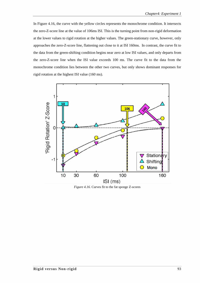
Chapter4: Experiment 1
Rigid versus Non-rigid 93
In Figure 4.16, the curve with the yellow circles represents the monochrome condition. It intersects
the zero-Z-score line at the value of 106ms ISI. This is the turning point from non-rigid deformation
at the lower values to rigid rotation at the higher values. The green-stationary curve, however, only
approaches the zero-Z-score line, flattening out close to it at ISI 160ms. In contrast, the curve fit to
the data from the green-shifting condition begins near zero at low ISI values, and only departs from
the zero-Z-score line when the ISI value exceeds 100 ms. The curve fit to the data from the
monochrome condition lies between the other two curves, but only shows dominant responses for
rigid rotation at the highest ISI value (160 ms).
Figure 4.16. Curves fit to the fat sponge Z-scores
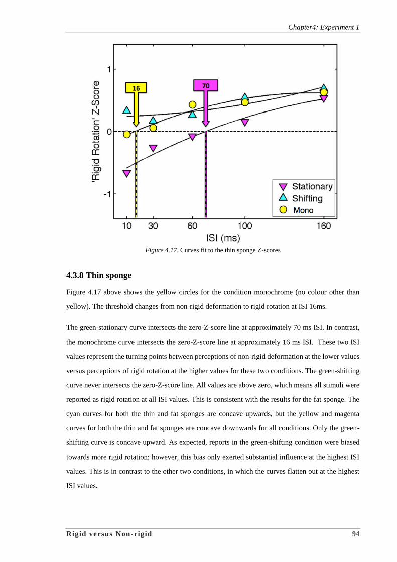
Chapter4: Experiment 1
Rigid versus Non-rigid 94
Figure 4.17. Curves fit to the thin sponge Z-scores
4.3.8 Thin sponge
Figure 4.17 above shows the yellow circles for the condition monochrome (no colour other than
yellow). The threshold changes from non-rigid deformation to rigid rotation at ISI 16ms.
The green-stationary curve intersects the zero-Z-score line at approximately 70 ms ISI. In contrast,
the monochrome curve intersects the zero-Z-score line at approximately 16 ms ISI. These two ISI
values represent the turning points between perceptions of non-rigid deformation at the lower values
versus perceptions of rigid rotation at the higher values for these two conditions. The green-shifting
curve never intersects the zero-Z-score line. All values are above zero, which means all stimuli were
reported as rigid rotation at all ISI values. This is consistent with the results for the fat sponge. The
cyan curves for both the thin and fat sponges are concave upwards, but the yellow and magenta
curves for both the thin and fat sponges are concave downwards for all conditions. Only the green-
shifting curve is concave upward. As expected, reports in the green-shifting condition were biased
towards more rigid rotation; however, this bias only exerted substantial influence at the highest ISI
values. This is in contrast to the other two conditions, in which the curves flatten out at the highest
ISI values.
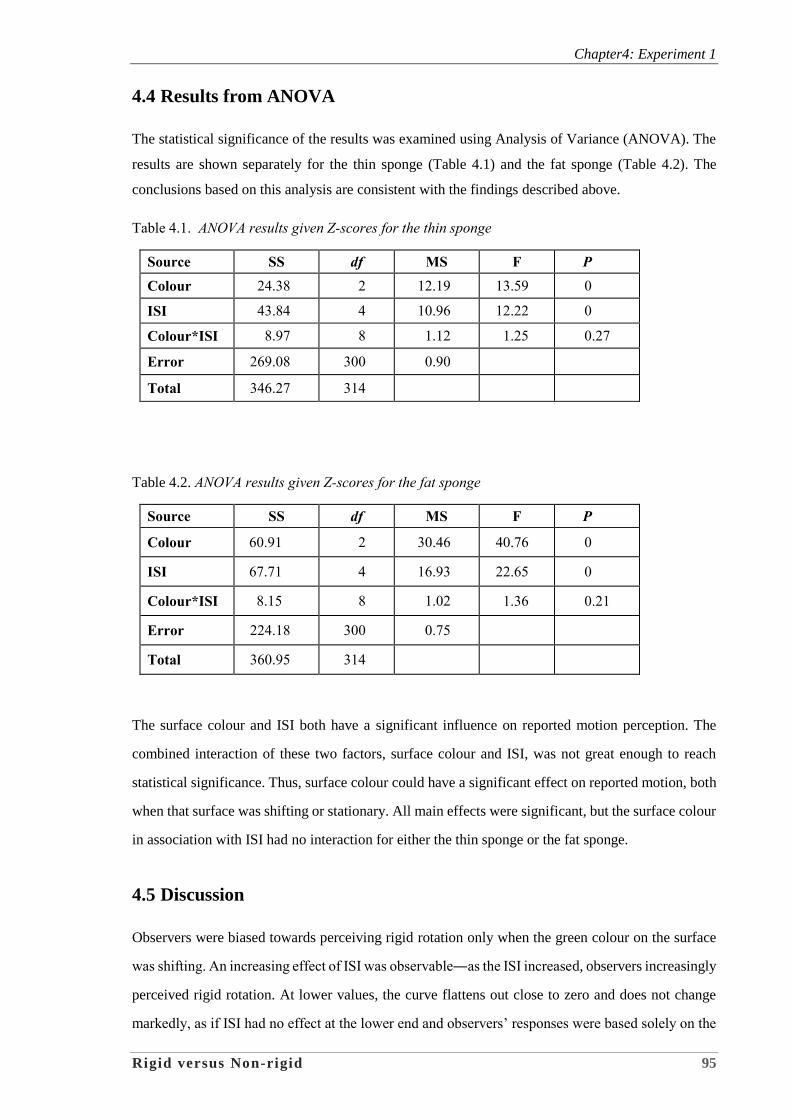
Chapter4: Experiment 1
Rigid versus Non-rigid 95
4.4 Results from ANOVA
The statistical significance of the results was examined using Analysis of Variance (ANOVA). The
results are shown separately for the thin sponge (Table 4.1) and the fat sponge (Table 4.2). The
conclusions based on this analysis are consistent with the findings described above.
Table 4.1. ANOVA results given Z-scores for the thin sponge
Source SS df MS F P
Colour 24.38 2 12.19 13.59 0
ISI 43.84 4 10.96 12.22 0
Colour*ISI 8.97 8 1.12 1.25 0.27
Error 269.08 300 0.90
Total 346.27 314
Table 4.2. ANOVA results given Z-scores for the fat sponge
Source SS df MS F P
Colour 60.91 2 30.46 40.76 0
ISI 67.71 4 16.93 22.65 0
Colour*ISI 8.15 8 1.02 1.36 0.21
Error 224.18 300 0.75
Total 360.95 314
The surface colour and ISI both have a significant influence on reported motion perception. The
combined interaction of these two factors, surface colour and ISI, was not great enough to reach
statistical significance. Thus, surface colour could have a significant effect on reported motion, both
when that surface was shifting or stationary. All main effects were significant, but the surface colour
in association with ISI had no interaction for either the thin sponge or the fat sponge.
4.5 Discussion
Observers were biased towards perceiving rigid rotation only when the green colour on the surface
was shifting. An increasing effect of ISI was observable―as the ISI increased, observers increasingly
perceived rigid rotation. At lower values, the curve flattens out close to zero and does not change
markedly, as if ISI had no effect at the lower end and observers’ responses were based solely on the
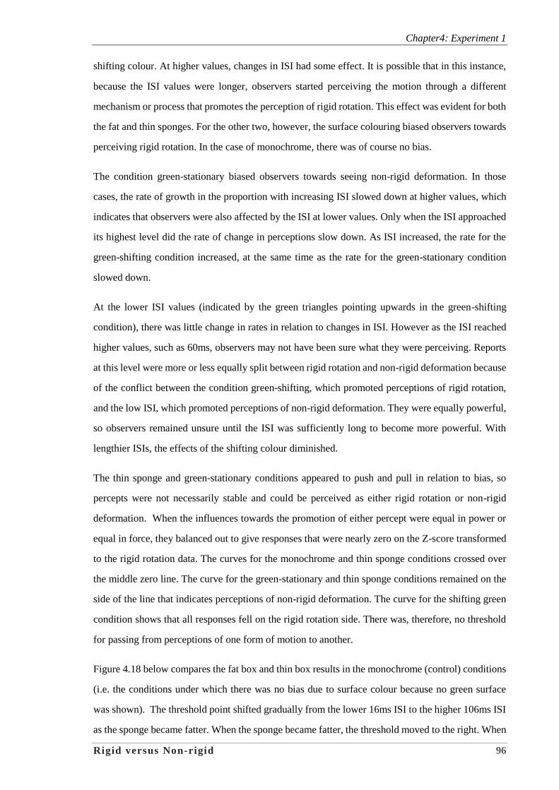
Chapter4: Experiment 1
Rigid versus Non-rigid 96
shifting colour. At higher values, changes in ISI had some effect. It is possible that in this instance,
because the ISI values were longer, observers started perceiving the motion through a different
mechanism or process that promotes the perception of rigid rotation. This effect was evident for both
the fat and thin sponges. For the other two, however, the surface colouring biased observers towards
perceiving rigid rotation. In the case of monochrome, there was of course no bias.
The condition green-stationary biased observers towards seeing non-rigid deformation. In those
cases, the rate of growth in the proportion with increasing ISI slowed down at higher values, which
indicates that observers were also affected by the ISI at lower values. Only when the ISI approached
its highest level did the rate of change in perceptions slow down. As ISI increased, the rate for the
green-shifting condition increased, at the same time as the rate for the green-stationary condition
slowed down.
At the lower ISI values (indicated by the green triangles pointing upwards in the green-shifting
condition), there was little change in rates in relation to changes in ISI. However as the ISI reached
higher values, such as 60ms, observers may not have been sure what they were perceiving. Reports
at this level were more or less equally split between rigid rotation and non-rigid deformation because
of the conflict between the condition green-shifting, which promoted perceptions of rigid rotation,
and the low ISI, which promoted perceptions of non-rigid deformation. They were equally powerful,
so observers remained unsure until the ISI was sufficiently long to become more powerful. With
lengthier ISIs, the effects of the shifting colour diminished.
The thin sponge and green-stationary conditions appeared to push and pull in relation to bias, so
percepts were not necessarily stable and could be perceived as either rigid rotation or non-rigid
deformation. When the influences towards the promotion of either percept were equal in power or
equal in force, they balanced out to give responses that were nearly zero on the Z-score transformed
to the rigid rotation data. The curves for the monochrome and thin sponge conditions crossed over
the middle zero line. The curve for the green-stationary and thin sponge conditions remained on the
side of the line that indicates perceptions of non-rigid deformation. The curve for the shifting green
condition shows that all responses fell on the rigid rotation side. There was, therefore, no threshold
for passing from perceptions of one form of motion to another.
Figure 4.18 below compares the fat box and thin box results in the monochrome (control) conditions
(i.e. the conditions under which there was no bias due to surface colour because no green surface
was shown). The threshold point shifted gradually from the lower 16ms ISI to the higher 106ms ISI
as the sponge became fatter. When the sponge became fatter, the threshold moved to the right. When

Chapter4: Experiment 1
Rigid versus Non-rigid 97
the sponge did not have a green side, only one surface colour (yellow) was presented for all the ISIs.
A smooth curve was fitted to the data points in order to identify the transition points between
perceived non-rigid deformation and more rigid rotation for each of the two object shapes. The
threshold intercept was shifted from 16ms to 106ms for the thin sponge and the fat sponge,
respectively. That is, for the thin sponge, the curve crosses over the zero line at 16ms, which is
between the two lowest ISI values (10ms and 30ms) presented during the experiments. In contrast,
for the fat sponge, the transition point is up around 106ms, which is between the two highest ISI
values (100ms and 160ms) presented during the experiments. This means that the fat object tended
to undergo more non-rigid deformation and the thin object tended to undergo more rigid rotation.
Figure 4.18. Curves fit to data for the fat vs. thin sponges in the monochrome condition (with no green side).
Two important findings should be noted here. The shape of the rectangular box undoubtedly
influenced which motion percept would be dominant. Rigid rotation was the dominant percept for
the thin sponge and non-rigid deformation was the dominant percept for the fat sponge. When rigid
rotation motion was the dominant percept (as it was for the thin sponge), only the condition of green-
stationary surface colour had a noticeable impact on the result, as the green-stationary surface colour
reinforced the non-rigid deformation percept. When non-rigid deformation motion was the dominant
percept (as it was for the fat sponge), only the green-shifting surface colour had a noticeable impact

Chapter4: Experiment 1
Rigid versus Non-rigid 98
on the result. This occurred because the shifting surface colour reinforced the rigid rotation percept
in contrast to the otherwise dominant deformation percept experienced for the thin sponge.
It can be concluded that patterns of surface colour variation (green-stationary, green-shifting and
monochrome) had a conditional influence on motion perception. The motion percept only changed
when the influence of the surface colour was opposite to the influence of the shape. Therefore, the
motion percept was modified only when the presented motion cues contradicted the dominant motion
percept observed in the control condition for each box (thin and fat). Tables 4.3 and 4.4 give a
parametric summary of the curve fitting for these two cases.
Table 4.3. Summary of the Curve fit to the Data for the Fat Sponge
Quadratic Linear Intercept
Thin_P1 = - 0.00005 0.016 - 1.30 Stationary
Thin_P2 = 0.00004 - 0.0020 0.04 Shifting
Thin_P3 = - 0.000024 0.012 - 1.01 Monochrome
Table 4.4. Summary of the Curve fit to the Data for the Thin Sponge
Quadratic Linear Intercept
Thin_P1 = - 0.000027 0.012 - 0.70 Green-
stationary
Thin_P2 = 0.000017 0.0003 0.24 Green-shifting
Thin_P3 = - 0.000034 0.0102 - 0.16 Monochrome
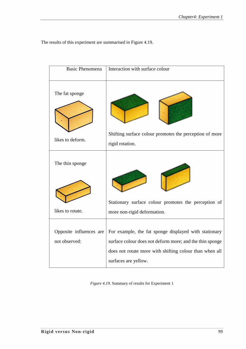
Chapter4: Experiment 1
Rigid versus Non-rigid 99
The results of this experiment are summarised in Figure 4.19.
Basic Phenomena Interaction with surface colour
The fat sponge
likes to deform.
Shifting surface colour promotes the perception of more
rigid rotation.
The thin sponge
likes to rotate.
Stationary surface colour promotes the perception of
more non-rigid deformation.
Opposite influences are
not observed:
For example, the fat sponge displayed with stationary
surface colour does not deform more; and the thin sponge
does not rotate more with shifting colour than when all
surfaces are yellow.
Figure 4.19. Summary of results for Experiment 1

Chapter5: Experiment 2
Rigid versus Non-rigid 100
CHAPTER 5: EXPERIMENT 2
5.1 Introduction
Experiment 2 was designed to show the nature and magnitude of potential adaptation after-effects on
the multi-stable motion percepts of rigid rotation versus non-rigid deformation. The hypothesis was
that prolonged viewing of a stimulus sequence that appears to rotate will decrease the amount of
rotation that will be seen during a subsequent test stimulus presentation. It was also hypothesised that
prolonged viewing of an adapting stimulus that appears to deform will decrease the amount of non-
rigid deformation that will be reported subsequent to adaptation.
As an aside note, some readers may be familiar with the use of the term adaptation to describes an
effect of brief duration that can be observed in the detection of subsequently viewed stimuli. For
example, in the study of the contrast thresholds for grating detection, thresholds are elevated for a
test grating presented 2.5 seconds after an adapting grating is presented for 5 seconds. In this context,
the use of the term adaptation indeed describes an effect of brief duration (Magnussen, et al.,1991;
Greenlee, et al.,1991). However, in the current study, the term adaptation is used to describe an
effect of prolonged viewing of adapting stimuli that can be observed for a much longer duration. This
use of the term adaptation is more common in studies of particular types of motion aftereffect (MAE)
that can be observed for a very long duration (Mather, et al., 1998). The aftereffects last for these
very long durations only after prolonged adaptation periods, such as those in the current experiment.
Many studies have can be found that have used comparably long adaptation periods over past half
century. For example, in early studies of direction-sensitive mechanisms, Pantle (1974) used the
term adaptation to describe the consequence of viewing of stimuli for 30 seconds that produce motion
aftereffects. More recently, Morgan (2012) measured MAE durations after 60 seconds of adaptation
to a display of expanding dots, an effect more closely associated with non-rigid deformation that
rigid rotation.
The trial structure of Experiment 2 involved two phases: adaptation and testing of the adaptation
after-effect. Two motion pecepts, rigid rotation (RR) and non-rigid deformation (ND), were
employed throughout the experiment. These were the same as those in Experiment 1. If the two-
process hypothesis was correct, then the following statement should also hold true: When adaptation
to stimulus (A) weakens the response of RR more than that of ND, there will be a decrease in the
proportion of reports of the first perceived motion (RR) after prolonged exposure to that stimulus.
Four different adapting stimuli were presented to 33 subjects. During the adaptation phase, the ISI
Chapter5: Experiment 2
Rigid versus Non-rigid 101
varied from trial to trial. The test phase was conducted after each trial to test the adaptation after-
effects.
5.2 Methods
5.2.1 Subjects
A total of 33 subjects was recruited from undergraduate and postgraduate students who were offered
a small inducement from funds provided by the University of Sydney. The majority ranged in age
from 19 to 33 years, with three observers aged between 46 and 66 years. There were eight female
and 25 male observers.
5.2.2 Design
Just as in Experiment 1, sessions in Experiment 2 were preceded by an orientation task. All observers
were given practice in reporting which of these two motion percepts was dominant during a prior test
session (this being the control condition session, which included no adaptation phase). This provided
a baseline against which adaptation after-effects could be measured and the extent to which after-
effects were caused by the prior adapting stimuli could be ascertained.
Each control-condition test session comprised seven blocks of six trials. One ISI value was presented
in each trial. All six ISI values were presented in random order within each block. Each observer
completed three such test sessions, so the total number of trials completed at each ISI was 21 (3
sessions x 7 blocks). First, 19 observers participated in the control- condition test sessions. In contrast
to Experiment 1, the control-condition test sessions used three sizes of rectangular boxes in order to
identify the most suitable size for Experiment 2. A medium sponge was added to the fat and thin
sponges. Its dimensions were 4:3:1.5.
Each adaptation-condition test session included two phases: adaptation and testing of the adaptation
after-effect. The first phase began with a 60s exposure to the adapting stimulus. During this initial
exposure, observers were required to attend to the adapting stimulus and report on which multi-stable
motion percept was experienced―rigid rotation or non-rigid deformation. After this initial exposure,
a block of test trials lasting approximately 20s was completed.
The second phase involved a 30s ‘refresher’ presentation of the adapting stimulus followed by the
same set of test trials but in random order and with a different ISI value. This second phase was
repeated three times. The trial structure of the experiment is shown in Figure 5.1.
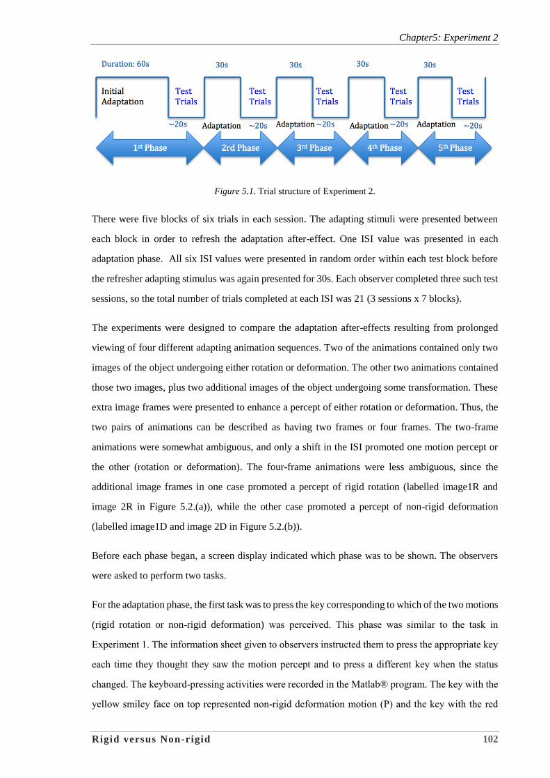
Chapter5: Experiment 2
Rigid versus Non-rigid 102
Figure 5.1. Trial structure of Experiment 2.
There were five blocks of six trials in each session. The adapting stimuli were presented between
each block in order to refresh the adaptation after-effect. One ISI value was presented in each
adaptation phase. All six ISI values were presented in random order within each test block before
the refresher adapting stimulus was again presented for 30s. Each observer completed three such test
sessions, so the total number of trials completed at each ISI was 21 (3 sessions x 7 blocks).
The experiments were designed to compare the adaptation after-effects resulting from prolonged
viewing of four different adapting animation sequences. Two of the animations contained only two
images of the object undergoing either rotation or deformation. The other two animations contained
those two images, plus two additional images of the object undergoing some transformation. These
extra image frames were presented to enhance a percept of either rotation or deformation. Thus, the
two pairs of animations can be described as having two frames or four frames. The two-frame
animations were somewhat ambiguous, and only a shift in the ISI promoted one motion percept or
the other (rotation or deformation). The four-frame animations were less ambiguous, since the
additional image frames in one case promoted a percept of rigid rotation (labelled image1R and
image 2R in Figure 5.2.(a)), while the other case promoted a percept of non-rigid deformation
(labelled image1D and image 2D in Figure 5.2.(b)).
Before each phase began, a screen display indicated which phase was to be shown. The observers
were asked to perform two tasks.
For the adaptation phase, the first task was to press the key corresponding to which of the two motions
(rigid rotation or non-rigid deformation) was perceived. This phase was similar to the task in
Experiment 1. The information sheet given to observers instructed them to press the appropriate key
each time they thought they saw the motion percept and to press a different key when the status
changed. The keyboard-pressing activities were recorded in the Matlab® program. The key with the
yellow smiley face on top represented non-rigid deformation motion (P) and the key with the red
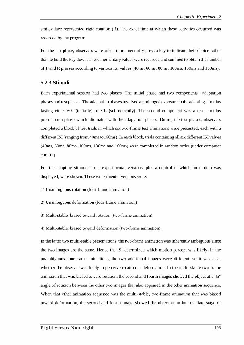
Chapter5: Experiment 2
Rigid versus Non-rigid 103
smiley face represented rigid rotation (R). The exact time at which these activities occurred was
recorded by the program.
For the test phase, observers were asked to momentarily press a key to indicate their choice rather
than to hold the key down. These momentary values were recorded and summed to obtain the number
of P and R presses according to various ISI values (40ms, 60ms, 80ms, 100ms, 130ms and 160ms).
5.2.3 Stimuli
Each experimental session had two phases. The initial phase had two components―adaptation
phases and test phases. The adaptation phases involved a prolonged exposure to the adapting stimulus
lasting either 60s (initially) or 30s (subsequently). The second component was a test stimulus
presentation phase which alternated with the adaptation phases. During the test phases, observers
completed a block of test trials in which six two-frame test animations were presented, each with a
different ISI (ranging from 40ms to160ms). In each block, trials containing all six different ISI values
(40ms, 60ms, 80ms, 100ms, 130ms and 160ms) were completed in random order (under computer
control).
For the adapting stimulus, four experimental versions, plus a control in which no motion was
displayed, were shown. These experimental versions were:
1) Unambiguous rotation (four-frame animation)
2) Unambiguous deformation (four-frame animation)
3) Multi-stable, biased toward rotation (two-frame animation)
4) Multi-stable, biased toward deformation (two-frame animation).
In the latter two multi-stable presentations, the two-frame animation was inherently ambiguous since
the two images are the same. Hence the ISI determined which motion percept was likely. In the
unambiguous four-frame animations, the two additional images were different, so it was clear
whether the observer was likely to perceive rotation or deformation. In the multi-stable two-frame
animation that was biased toward rotation, the second and fourth images showed the object at a 45°
angle of rotation between the other two images that also appeared in the other animation sequence.
When that other animation sequence was the multi-stable, two-frame animation that was biased
toward deformation, the second and fourth image showed the object at an intermediate stage of
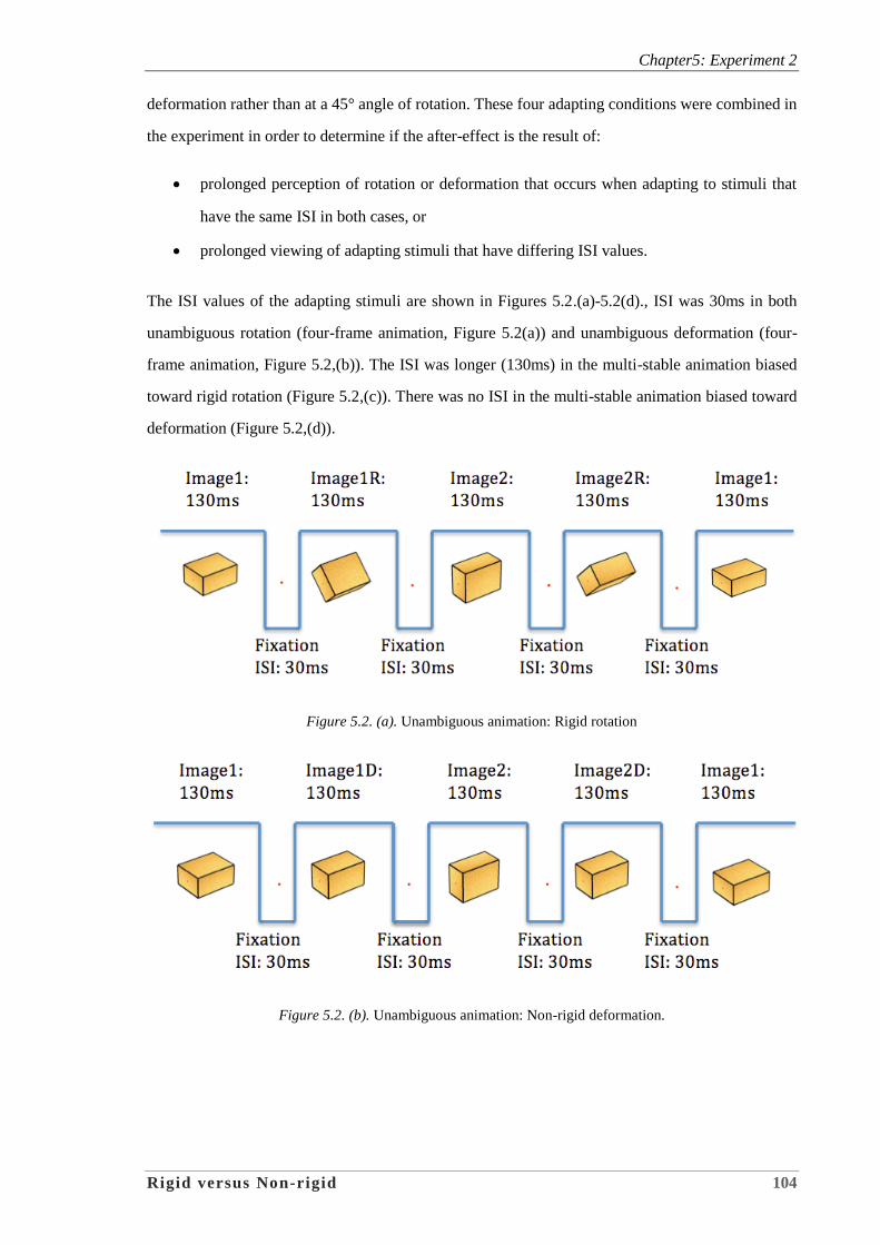
Chapter5: Experiment 2
Rigid versus Non-rigid 104
deformation rather than at a 45° angle of rotation. These four adapting conditions were combined in
the experiment in order to determine if the after-effect is the result of:
prolonged perception of rotation or deformation that occurs when adapting to stimuli that
have the same ISI in both cases, or
prolonged viewing of adapting stimuli that have differing ISI values.
The ISI values of the adapting stimuli are shown in Figures 5.2.(a)-5.2(d)., ISI was 30ms in both
unambiguous rotation (four-frame animation, Figure 5.2(a)) and unambiguous deformation (four-
frame animation, Figure 5.2,(b)). The ISI was longer (130ms) in the multi-stable animation biased
toward rigid rotation (Figure 5.2,(c)). There was no ISI in the multi-stable animation biased toward
deformation (Figure 5.2,(d)).
Figure 5.2. (a). Unambiguous animation: Rigid rotation
Figure 5.2. (b). Unambiguous animation: Non-rigid deformation.
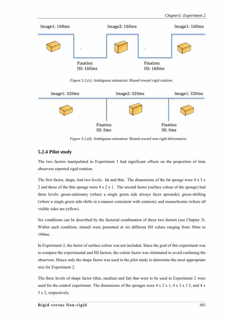
Chapter5: Experiment 2
Rigid versus Non-rigid 105
Figure 5.2.(c). Ambiguous animation: Biased toward rigid rotation.
Figure 5.2.(d). Ambiguous animation: Biased toward non-rigid deformation.
5.2.4 Pilot study
The two factors manipulated in Experiment 1 had significant effects on the proportion of time
observers reported rigid rotation.
The first factor, shape, had two levels: fat and thin. The dimensions of the fat sponge were 4 x 3 x
2 and those of the thin sponge were 4 x 2 x 1. The second factor (surface colour of the sponge) had
three levels: green-stationary (where a single green side always faces upwards); green-shifting
(where a single green side shifts in a manner consistent with rotation); and monochrome (where all
visible sides are yellow).
Six conditions can be described by the factorial combination of these two factors (see Chapter 3).
Within each condition, stimuli were presented at six different ISI values ranging from 30ms to
160ms.
In Experiment 2, the factor of surface colour was not included. Since the goal of this experiment was
to compare the experimental and ISI factors, the colour factor was eliminated to avoid confusing the
observers. Hence only the shape factor was used in the pilot study to determine the most appropriate
size for Experiment 2.
The three levels of shape factor (thin, medium and fat) that were to be used in Experiment 2 were
used for the control experiment. The dimensions of the sponges were 4 x 2 x 1, 4 x 3 x 1.5, and 4 x
3 x 2, respectively.
Chapter5: Experiment 2
Rigid versus Non-rigid 106
The results of the control experiment had indicated that the medium sponge should be the most
appropriate shape to use in Experiment 2. In the pilot study, however, the five observers who
participated saw mostly rigid rotation when using the medium sponge. This suggested that it was
difficult for them to see the shift at the intercept for the adaptation from the medium sponge.
Accordingly, it was decided to use the fat sponge in the pilot study instead. The results showed that
the two percepts (rigid rotation and non-rigid deformation) were more evenly observed with the
selected ISI range. Therefore, the fat sponge was selected for Experiment 2.
5.3 Results
The results are presented in two parts. The first part reports what observers perceived while viewing
the adapting stimuli from the four different animations. This was measured in terms of the length of
time during which the motion percepts were experienced. The second part reports what the observers
perceived in the test trials in which the ISI value was varied.
Results from the previous experiment showed that a simple stimulus parameter called Inter-stimulus
Interval (ISI) strongly influenced how much rigid rotation versus non-rigid deformation was seen.
This parameter could be varied by increasing or decreasing the time between the two frames of an
animation.
As previously explained, the ISI is the gap between when the image is shown and then taken away.
A long ISI, as defined here, is when an object in an image is shown for 160ms and then the object is
taken away for another 160ms, leaving only the fixation point. In this case, the object is visible on
the screen as long as it is off the screen.
The purpose of the experiment was to determine what influences the type of motion perceived when
an animated object is being shown. The animated object was always a rectangular box with a de-
formative character. When animated, the rectangular box can be seen as undergoing either rigid
rotation or non-rigid deformation.
The previous results showed that varying the ISI changed the relative proportion of the time that each
of the two motion percepts was reported. For example, when the ISI was set to 160ms, as shown in
Figure 5.3., most observers saw predominantly the rigid rotation percept.
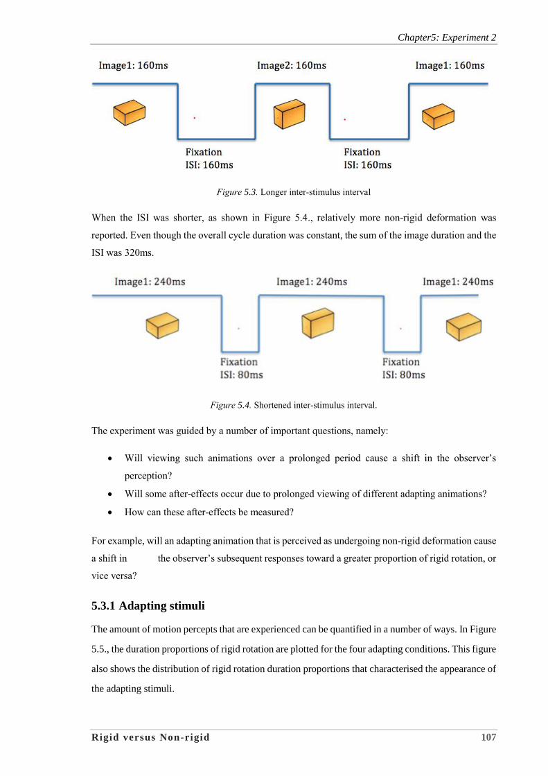
Chapter5: Experiment 2
Rigid versus Non-rigid 107
Figure 5.3. Longer inter-stimulus interval
When the ISI was shorter, as shown in Figure 5.4., relatively more non-rigid deformation was
reported. Even though the overall cycle duration was constant, the sum of the image duration and the
ISI was 320ms.
Figure 5.4. Shortened inter-stimulus interval.
The experiment was guided by a number of important questions, namely:
Will viewing such animations over a prolonged period cause a shift in the observer’s
perception?
Will some after-effects occur due to prolonged viewing of different adapting animations?
How can these after-effects be measured?
For example, will an adapting animation that is perceived as undergoing non-rigid deformation cause
a shift in the observer’s subsequent responses toward a greater proportion of rigid rotation, or
vice versa?
5.3.1 Adapting stimuli
The amount of motion percepts that are experienced can be quantified in a number of ways. In Figure
5.5., the duration proportions of rigid rotation are plotted for the four adapting conditions. This figure
also shows the distribution of rigid rotation duration proportions that characterised the appearance of
the adapting stimuli.
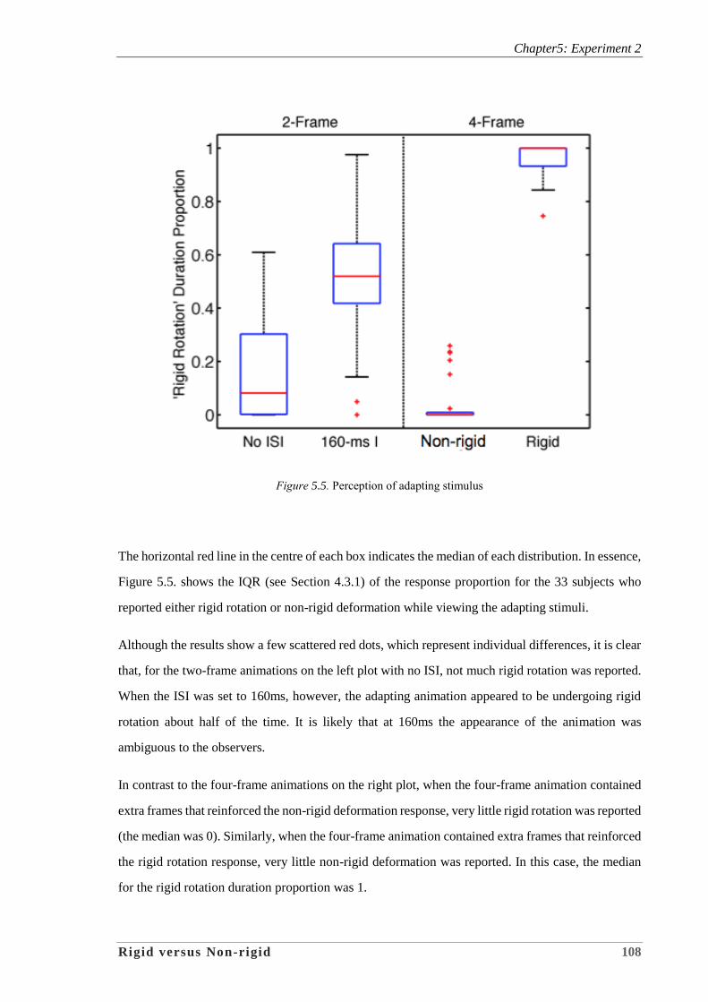
Chapter5: Experiment 2
Rigid versus Non-rigid 108
Figure 5.5. Perception of adapting stimulus
The horizontal red line in the centre of each box indicates the median of each distribution. In essence,
Figure 5.5. shows the IQR (see Section 4.3.1) of the response proportion for the 33 subjects who
reported either rigid rotation or non-rigid deformation while viewing the adapting stimuli.
Although the results show a few scattered red dots, which represent individual differences, it is clear
that, for the two-frame animations on the left plot with no ISI, not much rigid rotation was reported.
When the ISI was set to 160ms, however, the adapting animation appeared to be undergoing rigid
rotation about half of the time. It is likely that at 160ms the appearance of the animation was
ambiguous to the observers.
In contrast to the four-frame animations on the right plot, when the four-frame animation contained
extra frames that reinforced the non-rigid deformation response, very little rigid rotation was reported
(the median was 0). Similarly, when the four-frame animation contained extra frames that reinforced
the rigid rotation response, very little non-rigid deformation was reported. In this case, the median
for the rigid rotation duration proportion was 1.
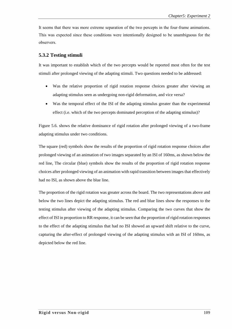
Chapter5: Experiment 2
Rigid versus Non-rigid 109
It seems that there was more extreme separation of the two percepts in the four-frame animations.
This was expected since these conditions were intentionally designed to be unambiguous for the
observers.
5.3.2 Testing stimuli
It was important to establish which of the two percepts would be reported most often for the test
stimuli after prolonged viewing of the adapting stimuli. Two questions needed to be addressed:
Was the relative proportion of rigid rotation response choices greater after viewing an
adapting stimulus seen as undergoing non-rigid deformation, and vice versa?
Was the temporal effect of the ISI of the adapting stimulus greater than the experimental
effect (i.e. which of the two percepts dominated perception of the adapting stimulus)?
Figure 5.6. shows the relative dominance of rigid rotation after prolonged viewing of a two-frame
adapting stimulus under two conditions.
The square (red) symbols show the results of the proportion of rigid rotation response choices after
prolonged viewing of an animation of two images separated by an ISI of 160ms, as shown below the
red line, The circular (blue) symbols show the results of the proportion of rigid rotation response
choices after prolonged viewing of an animation with rapid transition between images that effectively
had no ISI, as shown above the blue line.
The proportion of the rigid rotation was greater across the board. The two representations above and
below the two lines depict the adapting stimulus. The red and blue lines show the responses to the
testing stimulus after viewing of the adapting stimulus. Comparing the two curves that show the
effect of ISI in proportion to RR response, it can be seen that the proportion of rigid rotation responses
to the effect of the adapting stimulus that had no ISI showed an upward shift relative to the curve,
capturing the after-effect of prolonged viewing of the adapting stimulus with an ISI of 160ms, as
depicted below the red line.
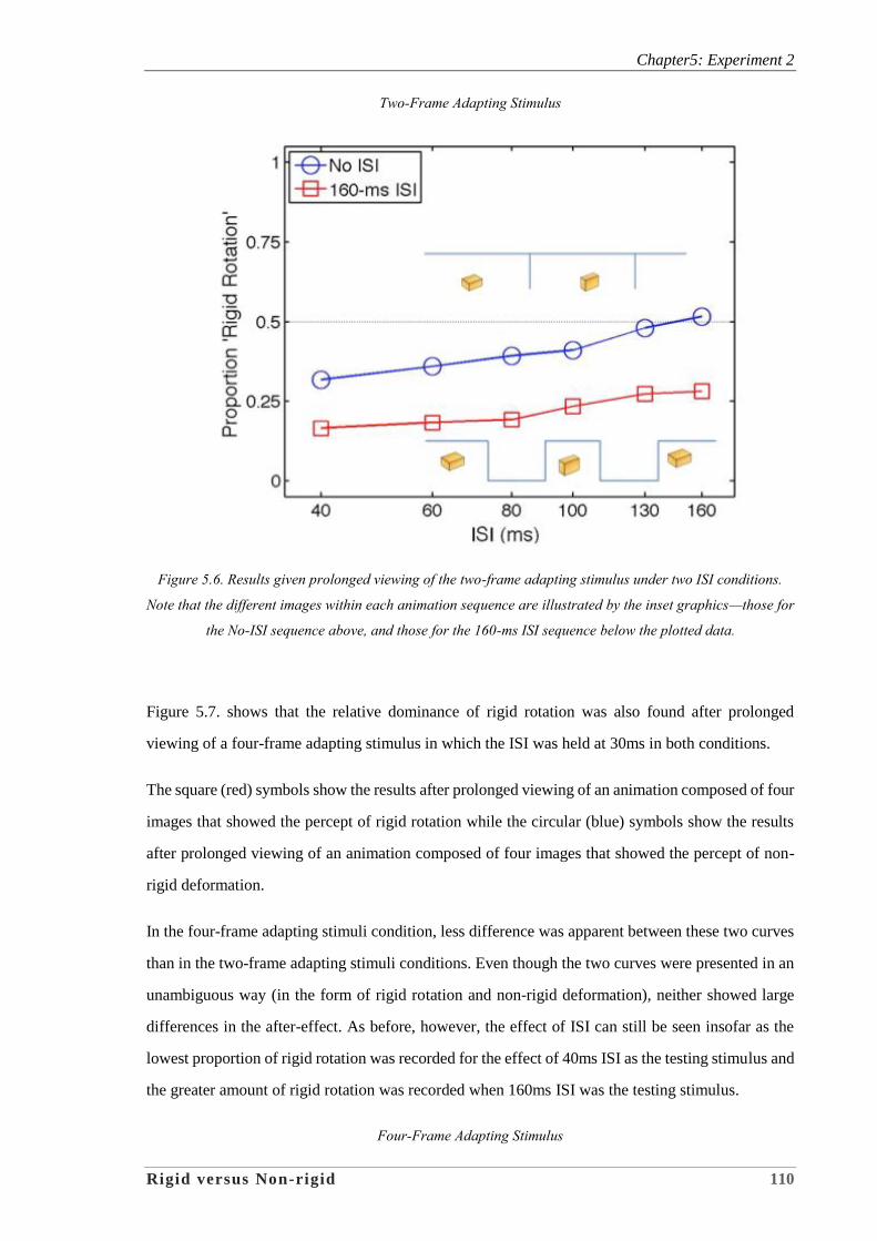
Chapter5: Experiment 2
Rigid versus Non-rigid 110
Two-Frame Adapting Stimulus
Figure 5.6. Results given prolonged viewing of the two-frame adapting stimulus under two ISI conditions.
Note that the different images within each animation sequence are illustrated by the inset graphics—those for
the No-ISI sequence above, and those for the 160-ms ISI sequence below the plotted data.
Figure 5.7. shows that the relative dominance of rigid rotation was also found after prolonged
viewing of a four-frame adapting stimulus in which the ISI was held at 30ms in both conditions.
The square (red) symbols show the results after prolonged viewing of an animation composed of four
images that showed the percept of rigid rotation while the circular (blue) symbols show the results
after prolonged viewing of an animation composed of four images that showed the percept of non-
rigid deformation.
In the four-frame adapting stimuli condition, less difference was apparent between these two curves
than in the two-frame adapting stimuli conditions. Even though the two curves were presented in an
unambiguous way (in the form of rigid rotation and non-rigid deformation), neither showed large
differences in the after-effect. As before, however, the effect of ISI can still be seen insofar as the
lowest proportion of rigid rotation was recorded for the effect of 40ms ISI as the testing stimulus and
the greater amount of rigid rotation was recorded when 160ms ISI was the testing stimulus.
Four-Frame Adapting Stimulus
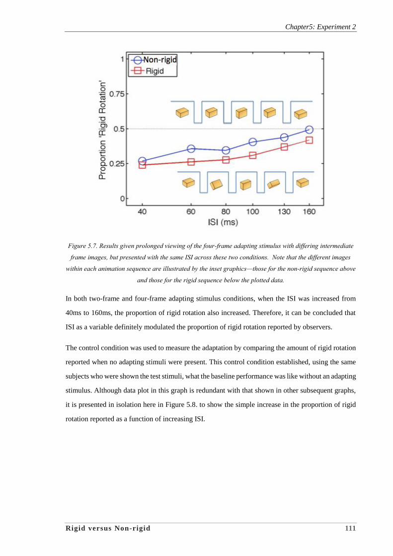
Chapter5: Experiment 2
Rigid versus Non-rigid 111
Figure 5.7. Results given prolonged viewing of the four-frame adapting stimulus with differing intermediate
frame images, but presented with the same ISI across these two conditions. Note that the different images
within each animation sequence are illustrated by the inset graphics—those for the non-rigid sequence above
and those for the rigid sequence below the plotted data.
In both two-frame and four-frame adapting stimulus conditions, when the ISI was increased from
40ms to 160ms, the proportion of rigid rotation also increased. Therefore, it can be concluded that
ISI as a variable definitely modulated the proportion of rigid rotation reported by observers.
The control condition was used to measure the adaptation by comparing the amount of rigid rotation
reported when no adapting stimuli were present. This control condition established, using the same
subjects who were shown the test stimuli, what the baseline performance was like without an adapting
stimulus. Although data plot in this graph is redundant with that shown in other subsequent graphs,
it is presented in isolation here in Figure 5.8. to show the simple increase in the proportion of rigid
rotation reported as a function of increasing ISI.
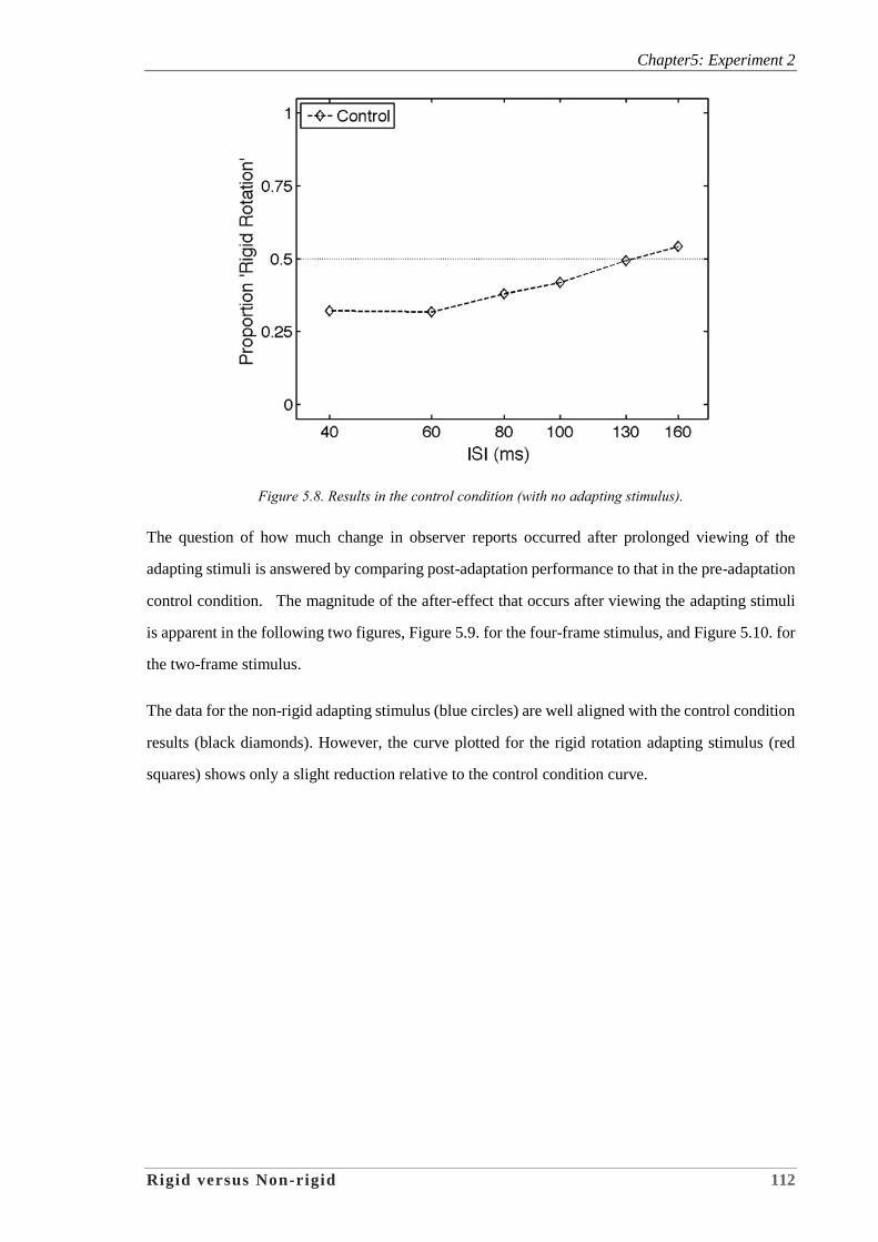
Chapter5: Experiment 2
Rigid versus Non-rigid 112
Figure 5.8. Results in the control condition (with no adapting stimulus).
The question of how much change in observer reports occurred after prolonged viewing of the
adapting stimuli is answered by comparing post-adaptation performance to that in the pre-adaptation
control condition. The magnitude of the after-effect that occurs after viewing the adapting stimuli
is apparent in the following two figures, Figure 5.9. for the four-frame stimulus, and Figure 5.10. for
the two-frame stimulus.
The data for the non-rigid adapting stimulus (blue circles) are well aligned with the control condition
results (black diamonds). However, the curve plotted for the rigid rotation adapting stimulus (red
squares) shows only a slight reduction relative to the control condition curve.
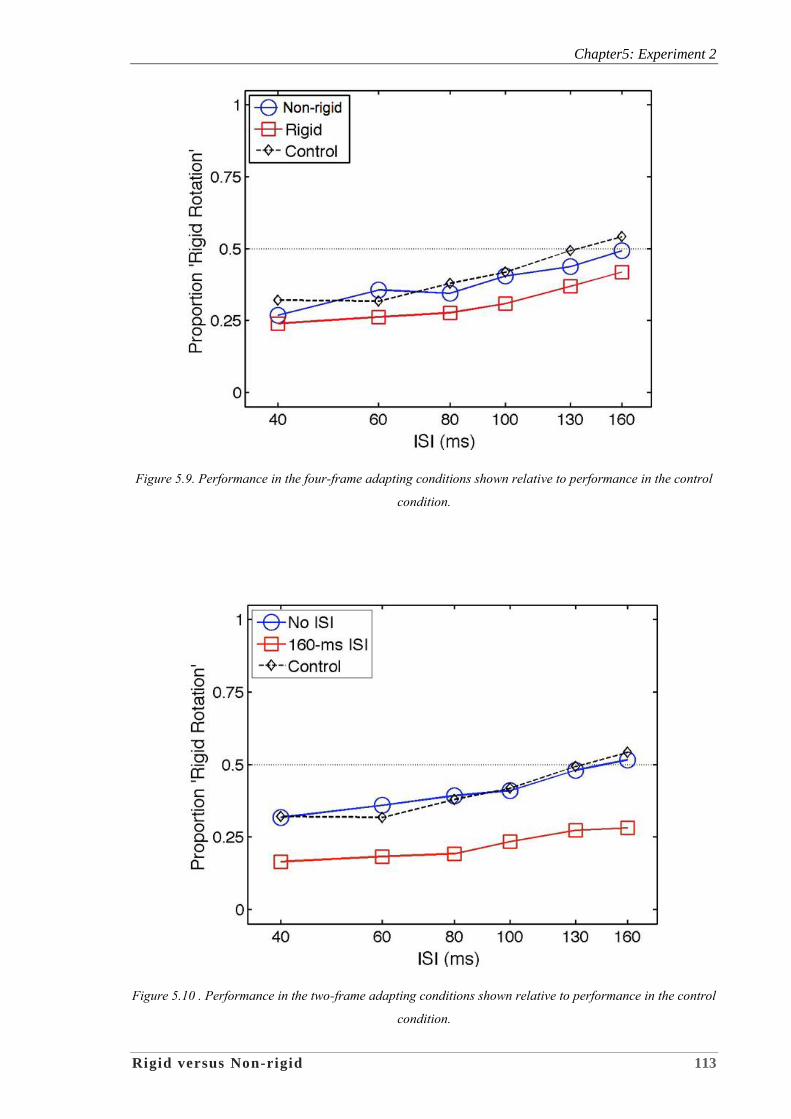
Chapter5: Experiment 2
Rigid versus Non-rigid 113
Figure 5.9. Performance in the four-frame adapting conditions shown relative to performance in the control
condition.
Figure 5.10 . Performance in the two-frame adapting conditions shown relative to performance in the control
condition.
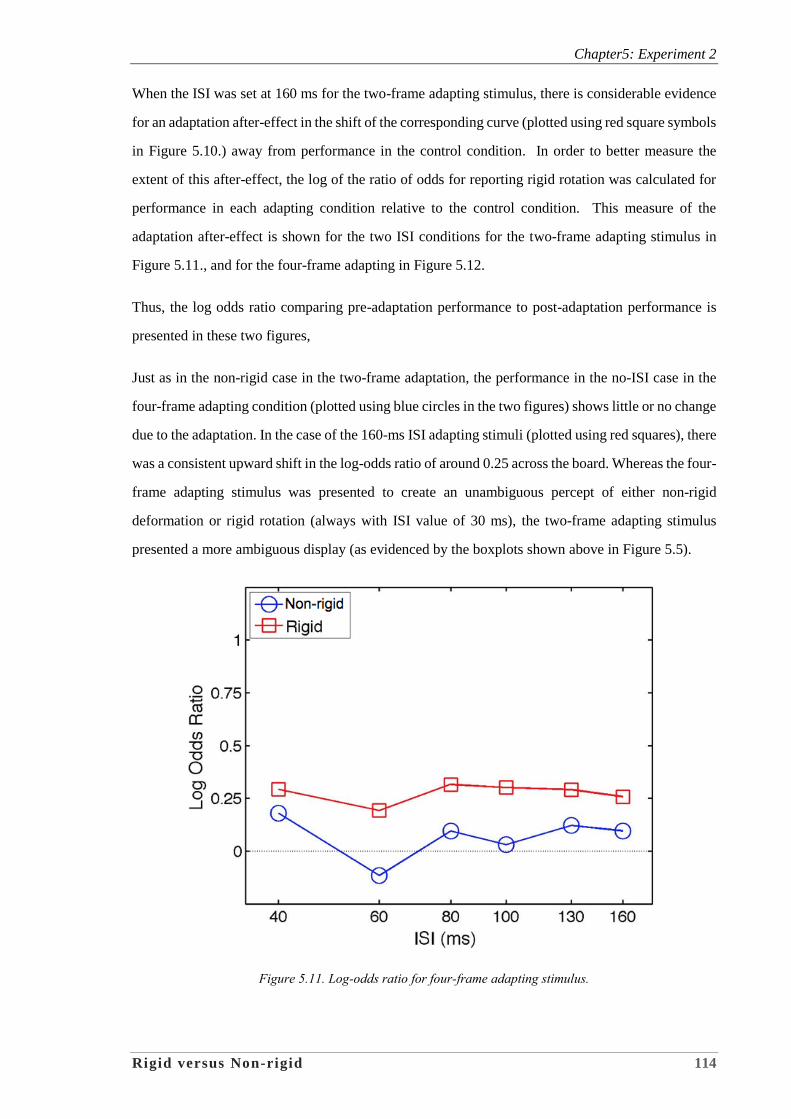
Chapter5: Experiment 2
Rigid versus Non-rigid 114
When the ISI was set at 160 ms for the two-frame adapting stimulus, there is considerable evidence
for an adaptation after-effect in the shift of the corresponding curve (plotted using red square symbols
in Figure 5.10.) away from performance in the control condition. In order to better measure the
extent of this after-effect, the log of the ratio of odds for reporting rigid rotation was calculated for
performance in each adapting condition relative to the control condition. This measure of the
adaptation after-effect is shown for the two ISI conditions for the two-frame adapting stimulus in
Figure 5.11., and for the four-frame adapting in Figure 5.12.
Thus, the log odds ratio comparing pre-adaptation performance to post-adaptation performance is
presented in these two figures,
Just as in the non-rigid case in the two-frame adaptation, the performance in the no-ISI case in the
four-frame adapting condition (plotted using blue circles in the two figures) shows little or no change
due to the adaptation. In the case of the 160-ms ISI adapting stimuli (plotted using red squares), there
was a consistent upward shift in the log-odds ratio of around 0.25 across the board. Whereas the four-
frame adapting stimulus was presented to create an unambiguous percept of either non-rigid
deformation or rigid rotation (always with ISI value of 30 ms), the two-frame adapting stimulus
presented a more ambiguous display (as evidenced by the boxplots shown above in Figure 5.5).
Figure 5.11. Log-odds ratio for four-frame adapting stimulus.
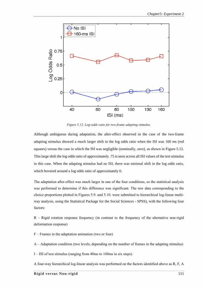
Chapter5: Experiment 2
Rigid versus Non-rigid 115
Figure 5.12. Log-odds ratio for two-frame adapting stimulus.
Although ambiguous during adaptation, the after-effect observed in the case of the two-frame
adapting stimulus showed a much larger shift in the log odds ratio when the ISI was 160 ms (red
squares) versus the case in which the ISI was negligible (nominally, zero), as shown in Figure 5.12.
This large shift the log odds ratio of approximately .75 is seen across all ISI values of the test stimulus
in this case. When the adapting stimulus had no ISI, there was minimal shift in the log odds ratio,
which hovered around a log odds ratio of approximately 0.
The adaptation after-effect was much larger in one of the four conditions, so the statistical analysis
was performed to determine if this difference was significant. The raw data corresponding to the
choice proportions plotted in Figures 5.9. and 5.10. were submitted to hierarchical log-linear multi-
way analysis, using the Statistical Package for the Social Sciences - SPSS), with the following four
factors:
R – Rigid rotation response frequency (in contrast to the frequency of the alternative non-rigid
deformation response)
F – Frames in the adaptation animation (two or four)
A – Adaptation condition (two levels, depending on the number of frames in the adapting stimulus)
I – ISI of test stimulus (ranging from 40ms to 160ms in six steps).
A four-way hierarchical log-linear analysis was performed on the factors identified above as R, F, A
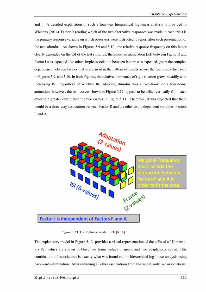
Chapter5: Experiment 2
Rigid versus Non-rigid 116
and I. A detailed explanation of such a four-way hierarchical log-linear analysis is provided in
Wickens (2014). Factor R (coding which of the two alternative responses was made in each trial) is
the primary response variable on which observers were instructed to report after each presentation of
the test stimulus. As shown in Figures 5.9 and 5.10., the relative response frequency on this factor
clearly depended on the ISI of the test stimulus; therefore, an association [RI] between Factor R and
Factor I was expected. No other simple association between factors was expected, given the complex
dependence between factors that is apparent in the pattern of results across the four cases displayed
in Figures 5.9. and 5.10. In both Figures, the relative dominance of rigid rotation grows steadily with
increasing ISI, regardless of whether the adapting stimulus was a two-frame or a four-frame
animation; however, the two curves shown in Figure 5.12. appear to be offset vertically from each
other to a greater extent than the two curves in Figure 5.11. Therefore, it was expected that there
would be a three-way association between Factor R and the other two independent variables, Factors
F and A.
Figure 5.13. The loglinear model: [RI] [RFA]
The explanatory model in Figure 5.13. provides a visual representation of the cells of a 3D matrix.
Six ISI values are shown in blue, two frame values in green and two adaptations in red. This
combination of associations is exactly what was found via the hierarchical log-linear analysis using
backwards elimination. After removing all other associations from the model, only two associations,
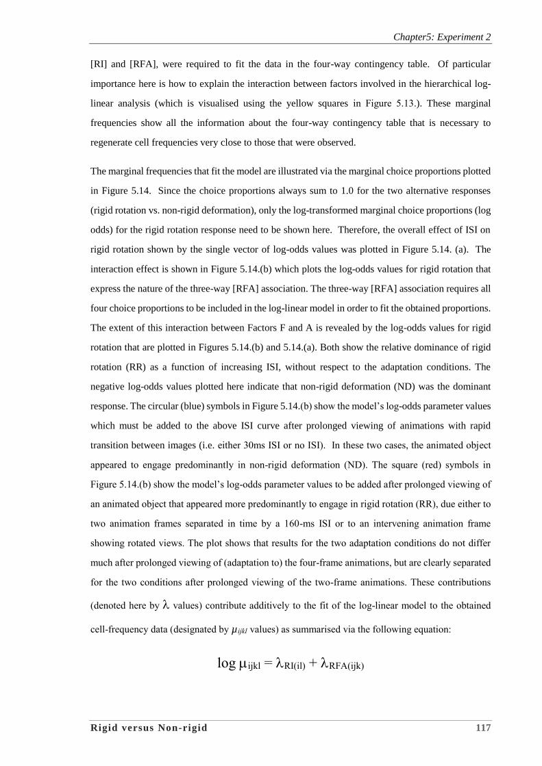
Chapter5: Experiment 2
Rigid versus Non-rigid 117
[RI] and [RFA], were required to fit the data in the four-way contingency table. Of particular
importance here is how to explain the interaction between factors involved in the hierarchical log-
linear analysis (which is visualised using the yellow squares in Figure 5.13.). These marginal
frequencies show all the information about the four-way contingency table that is necessary to
regenerate cell frequencies very close to those that were observed.
The marginal frequencies that fit the model are illustrated via the marginal choice proportions plotted
in Figure 5.14. Since the choice proportions always sum to 1.0 for the two alternative responses
(rigid rotation vs. non-rigid deformation), only the log-transformed marginal choice proportions (log
odds) for the rigid rotation response need to be shown here. Therefore, the overall effect of ISI on
rigid rotation shown by the single vector of log-odds values was plotted in Figure 5.14. (a). The
interaction effect is shown in Figure 5.14.(b) which plots the log-odds values for rigid rotation that
express the nature of the three-way [RFA] association. The three-way [RFA] association requires all
four choice proportions to be included in the log-linear model in order to fit the obtained proportions.
The extent of this interaction between Factors F and A is revealed by the log-odds values for rigid
rotation that are plotted in Figures 5.14.(b) and 5.14.(a). Both show the relative dominance of rigid
rotation (RR) as a function of increasing ISI, without respect to the adaptation conditions. The
negative log-odds values plotted here indicate that non-rigid deformation (ND) was the dominant
response. The circular (blue) symbols in Figure 5.14.(b) show the model’s log-odds parameter values
which must be added to the above ISI curve after prolonged viewing of animations with rapid
transition between images (i.e. either 30ms ISI or no ISI). In these two cases, the animated object
appeared to engage predominantly in non-rigid deformation (ND). The square (red) symbols in
Figure 5.14.(b) show the model’s log-odds parameter values to be added after prolonged viewing of
an animated object that appeared more predominantly to engage in rigid rotation (RR), due either to
two animation frames separated in time by a 160-ms ISI or to an intervening animation frame
showing rotated views. The plot shows that results for the two adaptation conditions do not differ
much after prolonged viewing of (adaptation to) the four-frame animations, but are clearly separated
for the two conditions after prolonged viewing of the two-frame animations. These contributions
(denoted here by values) contribute additively to the fit of the log-linear model to the obtained
cell-frequency data (designated by µijkl values) as summarised via the following equation:
log ijkl = RI(il) + RFA(ijk)
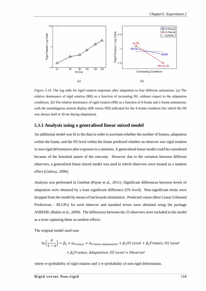
Chapter5: Experiment 2
Rigid versus Non-rigid 118
(a) (b)
Figure 5.14. The log odds for rigid rotation responses after adaptation to four different animations. (a) The
relative dominance of rigid rotation (RR) as a function of increasing ISI, without respect to the adaptation
conditions. (b) The relative dominance of rigid rotation (RR) as a function of 4-frame and 2-frame animations,
with the unambiguous motion display (RR versus ND) indicated for the 4-frame condition (for which the ISI
was always held at 30 ms during adaptation).
5.3.3 Analysis using a generalised linear mixed model
An additional model was fit to the data in order to ascertain whether the number of frames, adaptation
within the frame, and the ISI level within the frame predicted whether an observer saw rigid rotation
or non-rigid deformation after exposure to a stimulus. A generalised linear model could be considered
because of the binomial nature of the outcome. However due to the variation between different
observers, a generalised linear mixed model was used in which observers were treated as a random
effect (Galwey, 2006).
Analysis was performed in GenStat (Payne et al., 2011). Significant differences between levels of
adaptation were obtained by a least significant difference (5% level). Non-significant terms were
dropped from the model by means of backwards elimination. Predicted values (Best Linear Unbiased
Predictions - BLUPs) for each observer and standard errors were obtained using the package
ASREML (Butler et al., 2009). The differences between the 33 observers were included in the model
as a term capturing these as random effects.
The original model used was:
ln (𝜋
1 − 𝜋) = 𝛽0 + 𝛼𝐹𝑟𝑎𝑚𝑒𝑠 + 𝛼𝐹𝑟𝑎𝑚𝑒𝑠.𝐴𝑑𝑎𝑝𝑡𝑎𝑡𝑖𝑜𝑛 + 𝛽1𝐼𝑆𝐼 𝐿𝑒𝑣𝑒𝑙 + 𝛽2𝐹𝑟𝑎𝑚𝑒𝑠. 𝐼𝑆𝐼 𝐿𝑒𝑣𝑒𝑙
+ 𝛽3𝐹𝑟𝑎𝑚𝑒𝑠. 𝐴𝑑𝑎𝑝𝑡𝑎𝑡𝑖𝑜𝑛. 𝐼𝑆𝐼 𝐿𝑒𝑣𝑒𝑙 + 𝑂𝑏𝑠𝑒𝑟𝑣𝑒𝑟
where probability of rigid rotation and 1-probability of non-rigid deformation.
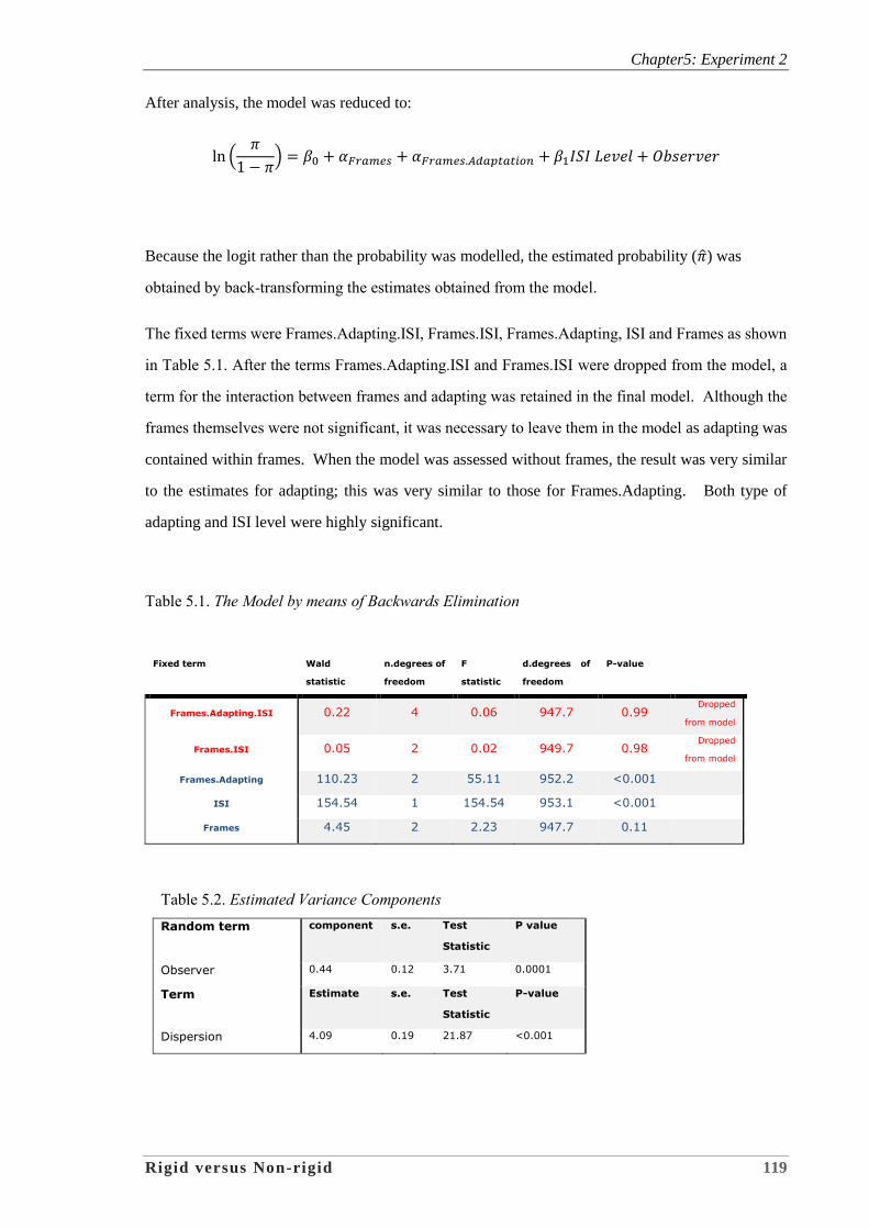
Chapter5: Experiment 2
Rigid versus Non-rigid 119
After analysis, the model was reduced to:
ln (𝜋
1 − 𝜋) = 𝛽0 + 𝛼𝐹𝑟𝑎𝑚𝑒𝑠 + 𝛼𝐹𝑟𝑎𝑚𝑒𝑠.𝐴𝑑𝑎𝑝𝑡𝑎𝑡𝑖𝑜𝑛 + 𝛽1𝐼𝑆𝐼 𝐿𝑒𝑣𝑒𝑙 + 𝑂𝑏𝑠𝑒𝑟𝑣𝑒𝑟
Because the logit rather than the probability was modelled, the estimated probability (�̂�) was
obtained by back-transforming the estimates obtained from the model.
The fixed terms were Frames.Adapting.ISI, Frames.ISI, Frames.Adapting, ISI and Frames as shown
in Table 5.1. After the terms Frames.Adapting.ISI and Frames.ISI were dropped from the model, a
term for the interaction between frames and adapting was retained in the final model. Although the
frames themselves were not significant, it was necessary to leave them in the model as adapting was
contained within frames. When the model was assessed without frames, the result was very similar
to the estimates for adapting; this was very similar to those for Frames.Adapting. Both type of
adapting and ISI level were highly significant.
Table 5.1. The Model by means of Backwards Elimination
Fixed term Wald
statistic
n.degrees of
freedom
F
statistic
d.degrees of
freedom
P-value
Frames.Adapting.ISI 0.22 4 0.06 947.7 0.99 Dropped
from model
Frames.ISI 0.05 2 0.02 949.7 0.98 Dropped
from model
Frames.Adapting 110.23 2 55.11 952.2 <0.001
ISI 154.54 1 154.54 953.1 <0.001
Frames 4.45 2 2.23 947.7 0.11
Table 5.2. Estimated Variance Components
Random term component s.e. Test
Statistic
P value
Observer 0.44 0.12 3.71 0.0001
Term Estimate s.e. Test
Statistic
P-value
Dispersion 4.09 0.19 21.87 <0.001
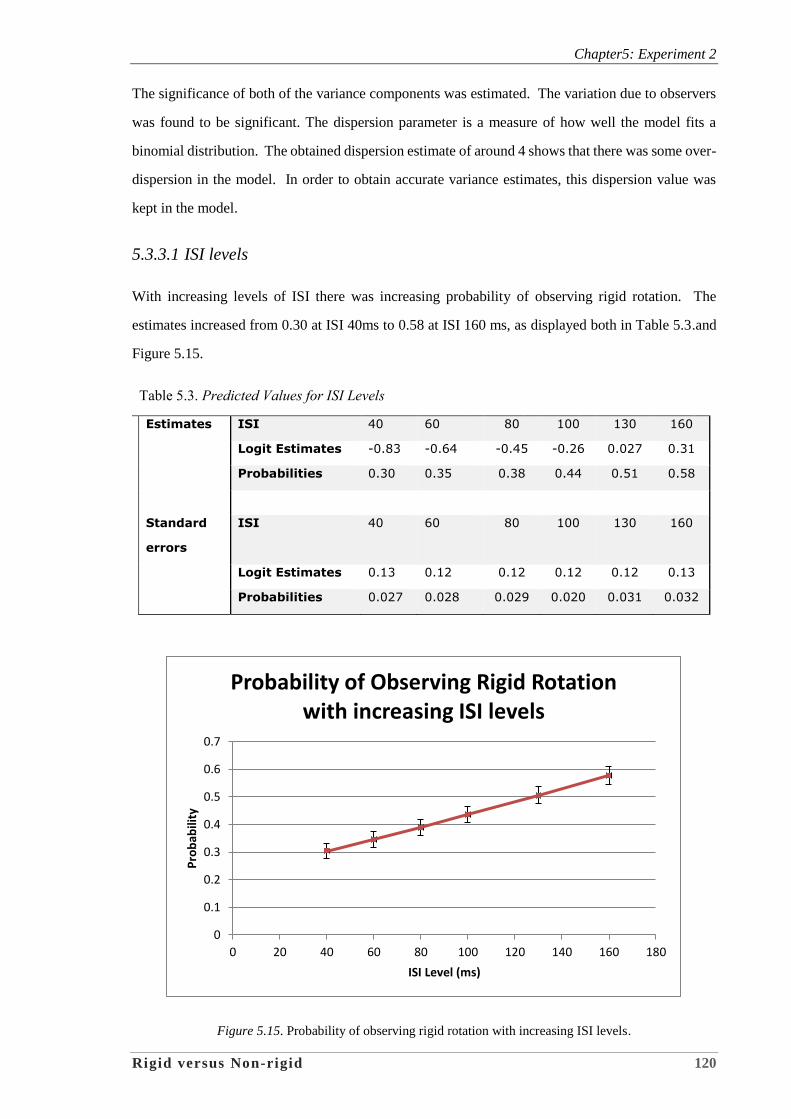
Chapter5: Experiment 2
Rigid versus Non-rigid 120
The significance of both of the variance components was estimated. The variation due to observers
was found to be significant. The dispersion parameter is a measure of how well the model fits a
binomial distribution. The obtained dispersion estimate of around 4 shows that there was some over-
dispersion in the model. In order to obtain accurate variance estimates, this dispersion value was
kept in the model.
5.3.3.1 ISI levels
With increasing levels of ISI there was increasing probability of observing rigid rotation. The
estimates increased from 0.30 at ISI 40ms to 0.58 at ISI 160 ms, as displayed both in Table 5.3.and
Figure 5.15.
Table 5.3. Predicted Values for ISI Levels
Estimates ISI 40 60 80 100 130 160
Logit Estimates -0.83 -0.64 -0.45 -0.26 0.027 0.31
Probabilities 0.30 0.35 0.38 0.44 0.51 0.58
Standard
errors
ISI 40 60 80 100 130 160
Logit Estimates 0.13 0.12 0.12 0.12 0.12 0.13
Probabilities 0.027 0.028 0.029 0.020 0.031 0.032
Figure 5.15. Probability of observing rigid rotation with increasing ISI levels.
0
0.1
0.2
0.3
0.4
0.5
0.6
0.7
0 20 40 60 80 100 120 140 160 180
Pro
bab
ility
ISI Level (ms)
Probability of Observing Rigid Rotation with increasing ISI levels
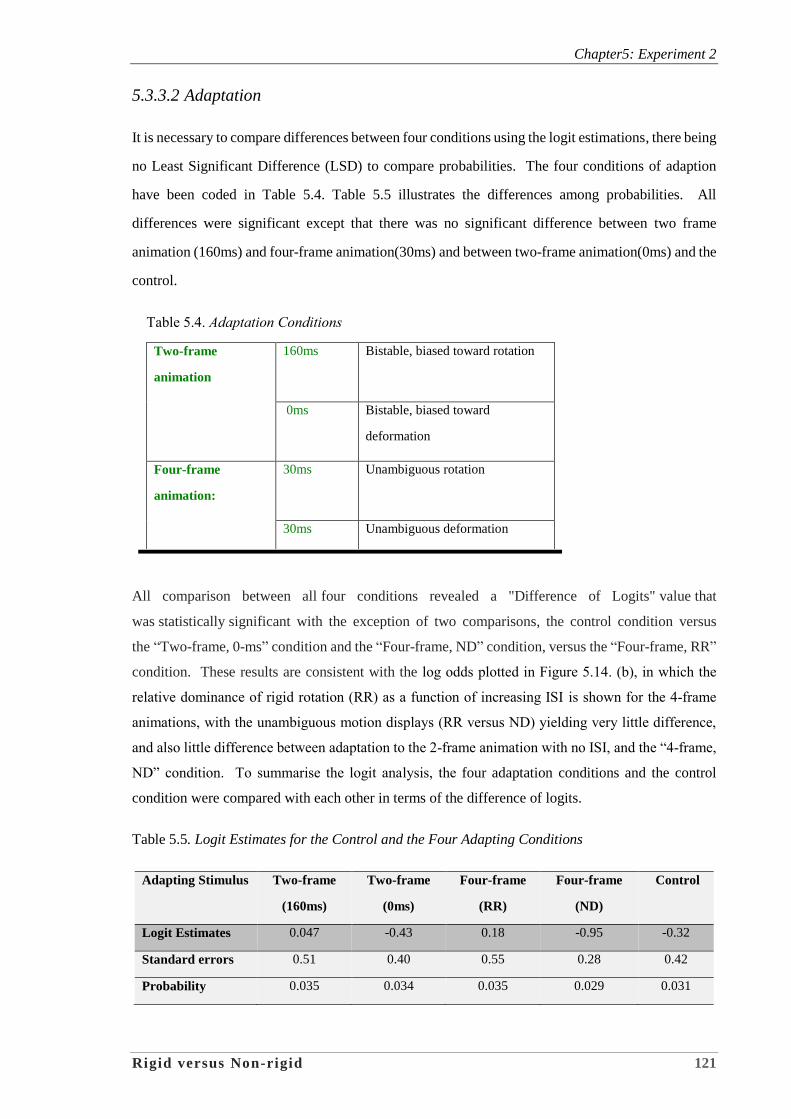
Chapter5: Experiment 2
Rigid versus Non-rigid 121
5.3.3.2 Adaptation
It is necessary to compare differences between four conditions using the logit estimations, there being
no Least Significant Difference (LSD) to compare probabilities. The four conditions of adaption
have been coded in Table 5.4. Table 5.5 illustrates the differences among probabilities. All
differences were significant except that there was no significant difference between two frame
animation (160ms) and four-frame animation(30ms) and between two-frame animation(0ms) and the
control.
Table 5.4. Adaptation Conditions
Two-frame
animation
160ms Bistable, biased toward rotation
0ms Bistable, biased toward
deformation
Four-frame
animation:
30ms Unambiguous rotation
30ms Unambiguous deformation
All comparison between all four conditions revealed a "Difference of Logits" value that
was statistically significant with the exception of two comparisons, the control condition versus
the “Two-frame, 0-ms” condition and the “Four-frame, ND” condition, versus the “Four-frame, RR”
condition. These results are consistent with the log odds plotted in Figure 5.14. (b), in which the
relative dominance of rigid rotation (RR) as a function of increasing ISI is shown for the 4-frame
animations, with the unambiguous motion displays (RR versus ND) yielding very little difference,
and also little difference between adaptation to the 2-frame animation with no ISI, and the “4-frame,
ND” condition. To summarise the logit analysis, the four adaptation conditions and the control
condition were compared with each other in terms of the difference of logits.
Table 5.5. Logit Estimates for the Control and the Four Adapting Conditions
Adapting Stimulus Two-frame
(160ms)
Two-frame
(0ms)
Four-frame
(RR)
Four-frame
(ND)
Control
Logit Estimates 0.047 -0.43 0.18 -0.95 -0.32
Standard errors 0.51 0.40 0.55 0.28 0.42
Probability 0.035 0.034 0.035 0.029 0.031
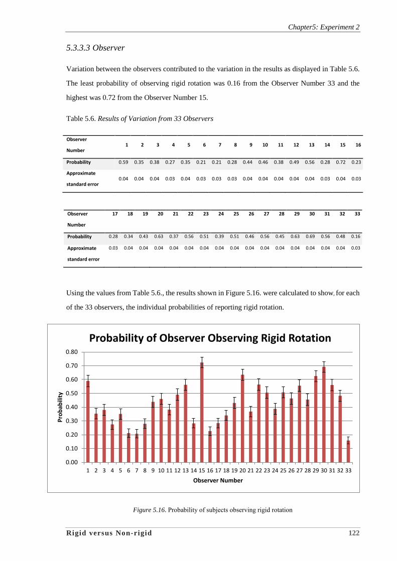
Chapter5: Experiment 2
Rigid versus Non-rigid 122
5.3.3.3 Observer
Variation between the observers contributed to the variation in the results as displayed in Table 5.6.
The least probability of observing rigid rotation was 0.16 from the Observer Number 33 and the
highest was 0.72 from the Observer Number 15.
Table 5.6. Results of Variation from 33 Observers
Observer
Number 1 2 3 4 5 6 7 8 9 10 11 12 13 14 15 16
Probability 0.59 0.35 0.38 0.27 0.35 0.21 0.21 0.28 0.44 0.46 0.38 0.49 0.56 0.28 0.72 0.23
Approximate
standard error 0.04 0.04 0.04 0.03 0.04 0.03 0.03 0.03 0.04 0.04 0.04 0.04 0.04 0.03 0.04 0.03
Observer
Number
17
18 19 20 21 22 23 24 25 26 27 28 29 30 31 32 33
Probability 0.28 0.34 0.43 0.63 0.37 0.56 0.51 0.39 0.51 0.46 0.56 0.45 0.63 0.69 0.56 0.48 0.16
Approximate
standard error
0.03 0.04 0.04 0.04 0.04 0.04 0.04 0.04 0.04 0.04 0.04 0.04 0.04 0.04 0.04 0.04 0.03
Using the values from Table 5.6., the results shown in Figure 5.16. were calculated to show, for each
of the 33 observers, the individual probabilities of reporting rigid rotation.
Figure 5.16. Probability of subjects observing rigid rotation
0.00
0.10
0.20
0.30
0.40
0.50
0.60
0.70
0.80
1 2 3 4 5 6 7 8 9 10 11 12 13 14 15 16 17 18 19 20 21 22 23 24 25 26 27 28 29 30 31 32 33
Pro
bab
ility
Observer Number
Probability of Observer Observing Rigid Rotation
Chapter 6: Discussion and Conclusion
Rigid versus Non-rigid 123
CHAPTER 6: DISCUSSION AND CONCLUSION
6.1 Discussion
This chapter discusses the results of two experiments on the bistable perception of apparent motion
associated with stroboscopic display of drawings of 3D objects, and presents several important
conclusions that can be drawn from those experiments. The overall results can be briefly summarised
as follows: Line drawings of rectangular boxes, with various surface colour schemes, were seen as
either rigidly rotating in space or as non-rigidly deforming, and changes in the relative dominance of
these two types of perceptual response were observed as a function of several variables. The most
powerful determinant of which response would likely dominate was the variable termed interstimulus
interval (ISI). This is a stimulus presentation parameter which, when increased, typically produced
an increase in the proportion of rigid rotation responses. Other factors that influenced the relative
proportion of rigid rotation over non-rigid deformation responses include the form of the presented
3D object and whether the position of a coloured surface on the 3D object shifted in a manner
consistent with rotation or not. The question that motivated the first of the two experiments
concerned the interaction between form and surface colour on the reported type of motion.
6.1.1 Experiment 1: Form and Surface Colour
The theories described in the introduction and the literature review chapters led to the formation of
a number of testable hypotheses regarding the role of form and surface colour in determining the
perceptual dominance of rigid rotation versus non-rigid deformation. First and foremost, however,
ISI was observed to be a most powerful influence on what type of motion an observer is likely to
perceive in stroboscopic display. In the context of the first experiment reported here, this first
hypothesis could be stated as follows: Increasing ISI should increase the proportion of time observers
report rigid rotation over non-rigid deformation.
Secondly, the form of the rectangular box was manipulated in the first experiment to be either fat or
thin, in order to test the hypothesis that change in the shape of the presented 3D object would shift
the point along the ISI continuum at which ‘rigid rotation’ responses become predominant. Previous
results presented in the literature review suggested that the fat rectangular box would lead observers
Chapter 6: Discussion and Conclusion
Rigid versus Non-rigid 124
to perceive non-rigid deformation, whereas the thinner rectangular box would bemore readily
perceive as rigidly rotating.
As explained in Chapter 1, non-rigid deformation does not change component vertex types between
frames, so it takes a shorter time to match the components from one frame to the other (where the
“component vertex types” are related to shape perception based on the theory of “recognition-by-
components” that was developed by Biederman, 1987). In rigid rotation, however, the component
vertex types change between frames, and it takes more time to process the difference between the
vertex types. The hypothesis tested in the first part of Experiment 1 (regarding the form of the
presented 3D object) was that fat rectangular box components tend to lead to deformation, while the
thin object tends to lead to rotation. The results were consistent with the propositions presented in
Chapter 1 and in Chapter 2, and have a rather straightforward explanation. Whereas visual
processing based on the rigidity assumption (Ullman, 1979, 1987) would tend to support ‘rotation’
responses, an examination of component vertex types reveals that the corresponding components of
the fat rectangular box travel a shorter local distance spatially, from frame 1 to frame 2, but the
corresponding components of the thin rectangular box must travel a longer distance between the
frames. Putting this more simply, it is easy to observe that the fat rectangular box undergoes only
minimum change as it deforms between frames, while the deformation of the thin rectangular box
entails a greater amount of change (with an edge 3-units in length shrinking to 1 unit, rather than 3-
unit edges shrinking to 2 units, as was the case for the fat rectangular box). In either case, the
deformation does not cause any change in the overall volume of the object, just as in the case of rigid
rotation. Other forms of deformation are no doubt less likely to show up as viable alternatives for
perception, and so the two mutually exclusive percepts are the only two that are reported under the
current experimental conditions. Suffice it to say that the above hypotheses are consistent with those
entertained in the literature reviewed in this thesis.
The two hypotheses noted above were tested under controlled conditions and can now be examined
based on the results of those tests. The variation in ISI, identified as the dominant sensory factor
here, had a significant influence on response proportions for both fat and thin rectangular boxes. As
has been found in many related cases (e.g., Gerbino, 1981), an increase in the ISI caused an increase
in the ‘rotation’ response. However, the thin box was seen as undergoing more rigid rotation at lower
ISI values than did the fat box. Indeed, the second hypothesis put forward here was thereby
Chapter 6: Discussion and Conclusion
Rigid versus Non-rigid 125
supported: The change in shape of the presented box would change the point along the ISI continuum
at which ‘rigid rotation’ responses become predominant.
These results suggest, unsurprisingly, that the stimulus timing factor ISI has a strong influence on
the visual perception of apparent motion. While the visual system operates according to several
competing principles, one of which is ‘minimum change’ in relation, for instance, to the preservation
of volume, there is an opportunity for factors that operate at a more cognitive level also to exert some
influence. Variation in the surface colour of the faces of the box was included here to provide for
the operation of such a cognitive factor. This factor was also manipulated in the first experiment so
as to either reinforce or contradict one or the other of the two alternative motion percepts.
In the first experiment, surface colour added an interesting element into the mix of factors
contributing to the predominance of one percept over another. The question to be examined here
was whether a low-level sensory factor, such as the ISI, might be more or less dominant than a higher-
level factor, such as the shift in position of the coloured faces of the rectangular box stimulus. Three
sets of conditions were constructed through the factorial combination of the two shapes with three
types of surface colour behaviour. The first was a monochrome presentation in which all surfaces
were a single colour (yellow). The other two presentations had one green face shifting either from
top to side (referred to as ‘green-shifting’), or remaining stationary on the top of the rectangular box
(‘green-stationary’). This allowed the following hypothetical questions to be addressed:
1. Does changing the surface colour of a stroboscopically displayed object affect the type of
perceived motion reported?
2. When the changing surface colour is consistent with rigid rotation, does this make a report of
rigid rotation more likely?
3. When the changing surface colour is inconsistent with rigid rotation, does this make a report of
rigid rotation less likely?
As was stated in Chapter 1 of this thesis, what is fascinating about these latter two questions is that
one might be answered in the affirmative while the other is answered in the negative. The preferred
hypothesis, as proposed here, was that the reported proportion of rigid rotation would not increase if
the surface colour of the object was made to shift under conditions in which the monochrome object
was already predominantly seen as rotating. Although the results of this first experiment (reported
in Chapter 3) clearly show that changing the surface colour of a stroboscopically displayed object
affects the type of perceived motion reported, the latter two questions did in fact have these opposing
answers under certain conditions: “no” to question 2 and “yes’ to question 3.
Chapter 6: Discussion and Conclusion
Rigid versus Non-rigid 126
Indeed, the results showed that, when the green surface remained stationary, observer responses were
only affected for the thin rectangular box; in contrast, when the green surface shifted, observer
responses were only affected for the fat rectangular box. These conditional influences are consistent
with the above-hypothesised dependencies. When rigid rotation was the dominant percept for the
thin sponge, adding the shifting green surface to the thin sponge might have promoted observers to
see more rigid rotation, but this did not happen in the case of the thin sponge. Rather, in the case of
the fat sponge, for which non-rigid deformation was the dominant percept, adding the shifting green
surface to the thin sponge led observers to see less non-rigid deformation. Conversely, non-rigid
deformation being the dominant percept for the fat sponge, adding a stationary green surface to the
fat sponge might have promoted the observers to see more non-rigid deformation, but this did not
happen either.
In summary, the results of the first experiment show how the display of the green surface could bias
observers to perceive more or less rigid rotation or non-rigid deformation. As discussed in the
previous chapters, the role of surface colour has been characterised as a cognitive factor, since the
observer’s knowledge about whether the object is rotating or deforming should be consistent with
the motion of the change in position of the green surface over time. First, the visual system seems
naturally to represent the rectangular box as a three dimensional (3D) object, even though it is only
presented as a two dimensional (2D) drawing on the screen, not as an actual three dimensional object.
Secondly, responses of observers seeing a rectangular box via the stroboscopic display with varying
surface colour were biased only under certain conditions. It seems that the conscious experience of
inconsistent surface colour variation can shift the proportion of responses under those conditions, but
does not influence responses when there is conscious experience of consistent surface colour
variation. This is regarded as a cognitive factor here based on the view that the peripheral sensory
system does not likely exhibit the kind of processing that would be responsible for the observed
surface colour bias. Rather, it is contended that an observer’s conscious knowledge of 3D object
behaviour is operating as an influence on what is consciously reported.
Apparent motion can be perceived without any analysis of form. Therefore, in some cases the
resulting apparent motion seems not to depend on the interpretation of what is seen by the observer,
because the observer is seeing motion without form, so there is no opportunity for interpretation
influencing reports. But if the observer sees a form first — for example, with a top surface that stays
green — then the likely interpretation is that the object with the green top has not rotated. The only

Chapter 6: Discussion and Conclusion
Rigid versus Non-rigid 127
other likely interpretation of the visual display is that it must have deformed, but this is not an obvious
consequence. Nonetheless, the form-based influence in this case seems to affect what is reported by
the observer, rather than the motion sensation that peripheral processing seems to be generating. This
is particularly clear in view of the fact that the influence is observed when the form-based factor
conflicts with the motion that might otherwise be perceived. When consistent with the motion the
observer was likely to perceive anyway, given the ISI, no modification of response proportions was
observed. However, if the observer saw something that was inconsistent, like the green patch staying
on the top of the stimulus when it would otherwise have been rotating, then a noticeable impact on
the results of response proportions was observed. Therefore, it can be concluded that the surface
colour variation had a conditional influence on motion perception when the observers were presented
with motion cues that contradicted the dominant motion percept in the control condition for the thin
and fat sponges. When ‘rigid rotation’ was the dominant percept for the thin sponge, only stationary
surface colour had a noticeable impact on the result, since stationary surface colour reinforced the
‘non-rigid deformation’ percept. When ‘non-rigid deformation’ was the dominant percept for the fat
sponge, only shifting surface colour had a noticeable impact on the result since shifting surface colour
reinforced the ‘rigid rotation’ percept.
Although some readers might regard the discussion of the results of such bistable perceptual studies
as incomplete without some treatment of the possible neural mechanisms that might be proposed to
underlie motion versus colour processing, such discussion has been explicitly stated as outside the
scope of this thesis questions. While it may be that the interaction between visual channels for motion
and colour processing is quite relevant particularly to the discussion of the results of Experiment 1,
it would be premature to attempt to extend the results of the current thesis to provide a basis for
developing further the popular model that would relates such perceptual and neural data. Readers
desiring to learn more about related neurophysiological models are directed to excellent review
of Viviani & Aymoz (2001).
6.1.2 Experiment 2: Adaptation
In the second experiment, adaptation after-effects were measured following prolonged viewing of
four adapting stimuli, in comparison to a control condition in which no adapting stimulus was
viewed. For two of the adapting stimuli, a common ISI value of 130 ms was used in two stroboscopic
presentations of two types of unambiguous motion. The other two adapting stimuli presented
ambiguous, multi-stable motion at two different ISI values. These four adapting stimuli were:
Chapter 6: Discussion and Conclusion
Rigid versus Non-rigid 128
1) Unambiguous rotation (four-frame animation), ISI of 130 ms.
2) Unambiguous deformation (four-frame animation), ISI of 130 ms.
3) Multi-stable, biased toward rotation (two-frame animation), ISI of 160 ms.
4) Multi-stable, biased toward deformation (two-frame animation), minimal ISI.
The following important hypotheses were posed in terms of adaptation after-effects:
Viewing such animations clearly displaying one sort of motion over a prolonged period can
cause a shift in the observer’s perception towards an alternative sort of motion.
Some variation in after-effects can occur due to prolonged viewing of adapting animations
that do not clearly display one sort of motion over another, and yet are predictable from
stimulus parameters such as ISI of the ambiguous adapting stimuli.
For example, an adapting animation that is perceived as undergoing non-rigid deformation can cause
a shift in the observer’s subsequent responses toward a greater proportion of rigid rotation, or vice
versa.
More particularly, the following hypotheses were tested by comparing post-adaptation responses to
these adapting stimuli:
The relative proportion of rigid rotation response choices increases after viewing an adapting
stimulus seen as undergoing non-rigid deformation, and vice versa.
The relative strength of an unobtrusive temporal factor, ISI of the adapting stimulus, can
under some conditions be greater than other experimental factors.
The results showed that the ISI in the adapting stimulus makes all the difference to what observers
report during the post-adaptation test phase, rather than what type of motion they reported
experiencing while viewing the adapting stimuli. One way to describe this phenomenon would be to
say that what the observers actually saw while viewing the adaptation stimuli could have influenced
what they later report seeing during the test phase, but the results of our experiments showed that the
after-effect is dominated by ISI. In fact, when the adapting stimuli were ambiguous, observers still
showed a strong after-effect that was consistent with the range of ISI values previously shown to be
associated with each type of motion—short ISI giving rise to more non-rigid deformation, long ISI
giving rise to more rigid rotation.
Chapter 6: Discussion and Conclusion
Rigid versus Non-rigid 129
After prolonged viewing of two unambiguous adapting stimuli, observers saw a great deal of rigid
rotation in the test phase after viewing non-rigid deformation. Likewise, they saw a great deal of
non-rigid deformation in the test phase after viewing rigid rotation. After prolonged viewing of an
ambiguous adapting stimulus with 160-ms ISI — one for which observers report seeing rotation half
of the time and deformation the other half of the time — it is worth questioning what effect the
observer’s subjective experience during adaptation should have on subsequent reports during the test
phase? The potentially surprising answer is “no effect,” which is nonetheless relatively easy to
explain if it is assumed that the ISI is one of the strongest determinants of the motion after-effects
under observation here. The explanation proceeds from the proposal that adapting to a long ISI will
fatigue the underlying mechanism, so that subsequent stimuli will exhibit less rigid rotation, even
though rotation was not a dominant percept during the adaptation period. Even after prolonged
viewing of an ambiguous adapting stimulus with no ISI — during which prolonged viewing the
perception of deformation is dominant — the observers’ subjective experiences during adaptation
still had little effect on subsequent reports during the test phase, which showed no shift in the relative
proportion of the two possible responses relative to the control condition in which no adaptation
stimuli were presented.
6.1.3 Comparison with Results from Other Studies
The ambiguity made these phenomena interesting. It seems that what is being perceived during
adaptation is less important than what is displayed, as ISI is the key factor in determining the resulting
after-effect. In the current study, the ISI was established clearly as a strong sensory factor that has a
dominant influence on the perception of apparent motion. A simple analogy can be made here is that
if people see two cars are racing, one car is in red colour and the other car is in black colour or any
colour other than red, although the speed for the two cars are the same, but people always think that
the red car is travelling faster than the other car. This case and the case of the current study share a
common underlying theme: what might seem to be an irrelevant factor (akin to car colour) dominates
the perception of the motion that is being seen. The reader also should be reminded of another study,
previously reviewed in this thesis, in which ambiguity during adaptation played a role. This was the
study on the role of attention in ambiguous reversals of structure-from-motion by Stonkute, Braun
and Pastukhov (2012), in which an adapting animation containing scattered (randomly positioned)
dots was presented such that some of the dots moved left to right (as if on the back surface of an
invisible sphere), and some of the dots moved right to left (as if on the front surface of a sphere).
Chapter 6: Discussion and Conclusion
Rigid versus Non-rigid 130
Because all the dots were of the same size, there was no bias one way or the other as to whether the
groups of dots moving in a common direction should be seen on the front or the rear surface of the
invisible sphere.
On each trial in that study, observers saw the distribution of randomly positioned dots as if on the
surface of an invisible sphere, with half of the dots rotating in one direction and the other half in the
other, and yet it is uncertain which set of dots was on the front surface. This ambiguous display was
used to determine what might bias observers to see the set of dots that were moving from right to left
as if they were on the front surface. One relevant manipulation that might bias the observer towards
this response was to make the dots slightly bigger when they are moving from right to left, so that
this subset of the dots would appear closer to the observer, adhering to the closer surface of the sphere
(i.e., the front of the sphere) instead of adhering to the back surface of the sphere. If the dots moving
from left to right on the surface of the sphere were made relatively smaller, that should then reinforce
the perception that those dots were adhering to the back surface of the sphere. These experiments by
Stonkute, Braun and Pastukhov (2012) examined how attention and stimulus parameters influence
outcomes of the forced ambiguous switch (FAS). It was found that poor attention to an ambiguously
rotating sphere, either due to competing attention-demanding tasks or due to natural fluctuations in
attentional state, resulted in fewer reversals of illusory motion. They found that illusory motion
reversals become more frequent if the sphere was comprised of fewer dots, was moving slower, or if
individual dots were further away from their opposing hemisphere counterpart at the time of FAS.
On the other hand, display properties strongly influenced ambiguous reversals. Colour cues were
manipulated in an experiment on perceptual ambiguity of rotating structure-from-motion displays.
These cues, when manipulated either by design or through by random dot placement, also shifted the
balance in favour of reversing illusory rotation (rather than depth). The conclusion drawn was that
the outcome of ambiguous reversals depended on attention, specifically on attention to the illusory
sphere and its surface irregularities, but not on attentive tracking of individual surface dots.
This type of investigation is analogous to the current investigation using the sponge as a stimulus in
that if a sponge was displayed with a stationary green patch on top, this detail influenced observers
to see more non-rigid deformation; and, vice versa, if a sponge was displayed with a shifting green
patch moving from its top to the side, then the observers were biased to see more rigid rotation. What
is similar between these two investigations? Without those cues of green coloured surface patches,
either shifting or stationary, an all-yellow sponge (with no biasing surface colour information) would

Chapter 6: Discussion and Conclusion
Rigid versus Non-rigid 131
be analogous to the spherical distribution of dots with no size difference giving rise to ambiguous
structure-from-motion display in the research of Stonkute Braun and Pastukhov (2012). Observers
would see a sphere covered in dots (the spherical structure derived from the coherent motion of the
dots), but since all of the dots are the same size (despite being on the front or back surface of the
implied sphere), no size cue operates to determine which dots are in front or back. This is analogous
to not colouring the surface of the sponge, but merely displaying an all-yellow sponge, so that only
the shape determines what is perceived. It will be shown that a fat sponge is more likely to be seen
in non-rigid deformation than a thin sponge, which is more likely to be seen in rigid rotation. What
we adapt to is the raw stimulus, regardless of what the interpretation was during the adaptation period.
The main consideration is what stimulus was presented to the observer, rather than what was
perceived by the observer.
This is distinct from the role of the observer’s interpretation during the measurement of motion after-
effects in Exner’s (1887) study. This study was described in Chapter 1, Section 1.2. The observer
in that study adapted to a moving pattern of horizontal lines while facing downward. Then, during
measurement of the after-effect, the observer either continued looking down or changed position to
look up towards a vertically displayed panel with the same horizontal lines on it. Although the
sensory component of the adaption after-effect was the same, the reported motion was different
simply because of the different orientation of the observer’s head. That is, when looking down, the
motion after-effect was in the opposite direction (“receding” rather than “approaching”), and yet was
reported as “moving upward” when the observer viewed the vertically displayed panel.
The motion after-effect was always observed to occur in a direction opposite from the pattern of the
stimulation on the retina during adaption. Although the viewing angle has been changed, the absolute
direction of motion in space is different from the absolute motion which would be expected in space
given the stimulus; however, given the relative orientation of the stimulus to the observer, the
reported direction of motion had changed by 90 degrees.
Exner (1887) makes a distinction between what is presented and what is experienced. What is
presented is just the stimulus, yet what is reported is influenced by the observer’s interpretation.
There was, however, an important difference between those results and the current study’s results, in
that the interpretation of the observers during the adaptation period was shown to have no influence
on what they reported during the measurement of the after-effect in the test phase.
Chapter 6: Discussion and Conclusion
Rigid versus Non-rigid 132
Here, an ambiguous stimulus presented during the adaptation period could be presented at two
extreme ISI values, and yet be perceived as undergoing mixed non-rigid deformation and rigid
rotation. Between the two adapting stimuli that were generally ambiguous, viewing the longer ISI
adapting stimulus gave rise to fewer reports of rigid rotation during the test phase, and so it was
concluded that the longer ISI affected one underlying mechanism more than the other. It can be
concluded then that what was displayed mattered more than what was perceived during the adaptation
period.
What the current experiment presented during adaptation to the ambiguous two-frame animations
resulted in a bistable percept in both cases, only slightly dependent on ISI. In fact, when there was
an extremely short ISI during the adapting phase, the observers did report more non-rigid
deformation, yet they also reported a substantial proportion of rigid rotation responses. Nonetheless,
the after-effect of viewing both of these ambiguous stimuli was quite strongly dependent on the
adapting ISI value. The results showed a strong after-effect from viewing the long-ISI adapting
stimulus, just as if observers had been seeing lots of rigid rotation. But during the adaptation period
in this case, observers reported both types of motion for about half of the time—half of the time
reporting rigid rotation and half of the time reporting non-rigid deformation.
Were the findings reported here unusual, or do other studies of apparent motion show similar results?
Results from Anstis and Moulden (1970) showed a strong adaptation after-effect to a specially
controlled apparent motion display which, they concluded, was based on the “seen motion” rather
than stimulus parameters, which were held constant in their experiments. In contrast to the current
results, the results of Anstis and Moulden (1970) indicate a relatively stronger influence of what is
“seen” (the perceptual phenomenon) than what is displayed (the physical stimulus). It should be
noted that those experiments were designed to test central versus peripheral components producing
motion after-effects, which was not addressed in the current experiments. A study that did examine
central versus peripheral components of adaption was reported by Exner (1887), as discussed above.
Suffice it to say here that Exner (1887) had a very similar idea in distinguishing what was presented
from what was experienced (although he used different terms). His results, however, do not suggest
that what was “seen” during adaptation made a stronger difference in what would be reported after
adaptation than what was presented; rather, his results suggest that the interpretation of the observer
during the measurement of the after-effect is a critical factor to be considered.
Chapter 6: Discussion and Conclusion
Rigid versus Non-rigid 133
Caplovitz (2007) also did a similar study using rotating dotted ellipses. In his study, a rotating ellipse
could be perceived as either rigid (thinner ellipse) or non-rigid (fatter ellipse). It was noticed that for
an intermediate aspect ratio ellipse, the percept will often start out as rigid and then transition to non-
rigid. Once non-rigid, the percept will stay there and not revert back to rigid. It was reported that
over prolonged viewing of looking at various ambiguous stimuli, the observers tend to learn to see
one percept more readily. A mid-aspect ratio ellipse, once experienced as non-rigid, would, after
once being seen as rigid to the observer, would from then on tend to appear to be rigid. In an extreme
case, a video was made of an elliptical contour made up of evenly spaced dots. The results showed
that ellipses defined by closely spaced dots exhibit the speed illusion observed with continuous
contours (Caplovitz, 2007). That is, thin dotted ellipses displayed to be rotating faster than fat dotted
ellipses when both rotating at the same angular velocity. However, this illusion was not observed if
the dots defining the ellipse were spaced too widely apart. A control experiment was conducted to
ensure that low spatial frequency "blurring" was not the source of the illusory percept. In conclusion,
even in the presence of local motion signals that are immune to the aperture problem, the global
percept of an ellipse undergoing rotation can be driven by potentially ambiguous motion signals
arising from the non-local form of the grouped ellipse itself. Here motion perception is driven by
emergent motion signals such as those of virtual contours constructed by grouping procedures.
As in the discussion on low level and high level processes in Chapter 1.3, the low level process was
presumedly operating when local pairs of dots would stay in the center and observers perceived
element motion. However, after some time this pairing forced the extreme components appear to
jump further, potentially engaging the high-level, long-range process, which lead to the perception
of group motion. These findings showed that it was very hard to see the ‘local’ motion details after
prolonged viewing (perhaps adapting at a lower level), which came to be dominated by the more
‘global’ or ‘active’ percept. These findings can be related to the findings of the current study in that
the stimulus ambiguity arises from a clash between the lower level percept and a more ‘global’ or
‘active’ percept. In the current after-effect study, when the adapting stimuli were ambiguous,
observers still showed a strong shift in the response proportions for each type of motion as ISI values
were manipulated. After prolonged viewing at short ISI, during which period the non-rigid
deformation is more likely, a shift towards rigid rotation will certainly become more dominant, but
not necessarily due to observers seeing more non-rigid deformation during the adaptation period.
This result might be explained if the motion percept is more strongly determined by the factors that
trigger the low level (local) process versus the high level (global) process in apparent motion, rather
Chapter 6: Discussion and Conclusion
Rigid versus Non-rigid 134
than cognitive factors that would by modulated by what was “seen” rather than what was “displayed”
in a given condition.
6.2 Conclusion
It was expected that ISI would be the dominant factor influencing the relative proportion of ‘rigid
rotation’ versus ‘non-rigid deformation’ in the bistable stroboscopic motion display investigated
here. It was, however, harder to predict the influence of surface colour on these ISI-dependent
responses. The current findings showed that changing the surface colour of the object between
stroboscopically displayed stimulus frames only influenced responses when the changes in surface
colour contradicted the predominant response for a stimulus at a given ISI value. This might be
somewhat surprising for readers, but even more surprising was that this temporal factor describing
an adapting stimulus (i.e., ISI) was more powerful than the experiential factor associated with the
adapting stimulus (i.e., what motion was actually perceived during the adaptation period). This
experiential factor was monitored continuously during the adaptation period, so it was clear what
proportion of the time each of the two motion percepts was being experienced in each adapting
condition. Yet the reported percepts indicated that what observers experienced during adaptation
did not have the expected impact on the subsequent perception of a test stimulus, which would be to
shift the relative proportion of a given response toward the alternative response (i.e., opposite to that
experienced during adaption). Instead, prolonged viewing of a given stimulus resulted in an
adaptation after-effect that was predictable from the ISI of the adapting stimulus, regardless of what
observers reported they had seen while viewing the adaptation stimulus.
These results are consistent with many of the theoretical concepts examined in the literature review
of this thesis, such as those associated with the rigidity assumption (Ulman, 1979; 1983), recognition-
by-components (Biederman, 1987), and the hypothesised association field (Field, 1993; Alais and
Lorenceau, 2002). The hypothetical principles supported by previous findings can explain some of
the current results, but these principles do not always explain what will determine which reported
motion will predominate. For example, it was difficult to predict the extent to which the fatter of
two presented rectangular boxes would produce a dominant ‘non-rigid deformation’ response.
Consistent with a ‘preservation of volume’ assumption, this dominance can be explained according
to the close proximity between corresponding components, the corners of the fat rectangular box,
with the box undergoing only minimum change as it deforms between frames. In contrast, the
deformation of the thin rectangular box entails a greater amount of change from frame 1 to frame 2,
Chapter 6: Discussion and Conclusion
Rigid versus Non-rigid 135
so a dominant ‘rigid rotation’ response would be regarded as less likely from the ‘corresponding
components’ perspective, with corners of the thin rectangular box traveling a greater spatial distance
between the frames. This result is consistent with results typically observed with the Ternus display,
but in this case the shorter ISI is associated with more non-rigid deformation, due to local processes,
in that here the longer ISI promotes more rigid rotation, due to a more global motion process (which
may also require greater time to develop, in comparison to non-rigid deformation). Nonetheless, the
superficial appearance of the object could influence the response proportions when a dissonance
between colour and motion exists due to shifts in the colour of the faces of the presented rectangular
boxes.
Despite the clear influence of this dissonance in cognition on results obtained in the first experiment,
the results of the second experiment showed the greater importance of the ISI, a relatively
unobtrusive stimulus factor. It is tempting to speculate about the role of the ISI in pre-attentive
processing (Treisman, 1986; Lamme and Roelfsema, 2000), which might be regarded as consistent
with the two process model as formulated by Pantle and Picciano (1976) and others (Braddick, 1973
& 1974; Gerbino, 1981). Even at a level of processing that might be regarded as cognitive, however,
there are similar ideas of relatively unconscious processing that proceeds in an apparently iterative
manner in testing perceptual hypotheses, such as Neisser’s (1978) perceptual cycle. Suffice it to say
that there is more work to be done to reveal the nature of the processing underlying such percepts as
non-rigid deformation and rigid rotation, regardless of whether observers have introspective access
to the dominant stimulus variables or not.
6.3 Future Work
An obvious further experiment that could be executed with additional equipment would be to
compare the different viewing conditions enabled by stereoscopic display. Many important studies
of the two process model have included single-eye versus two-eye presentations of stroboscopic
stimuli in order to determine whether some processing is occurring at a more peripheral or a more
central level. For example, Pantle and Picciano’s (1976) work (see detailed discussion in Chapter
2, Section 2.2.1) suggested that the element process generated movement signals at a peripheral level
of processing, while the group process seemed to function at a more central level in the binocular
visual system. When manipulating the duration of the ISI, they observed changes in the relative
proportion of group and element movement under binocular viewing conditions. Under dichoptic
viewing conditions, in which the two frames of the display were viewed in alternation by each of the
Chapter 6: Discussion and Conclusion
Rigid versus Non-rigid 136
two eyes, virtually no element movement was reported. In a similar study (Gerbino, 1981), flat
triangular elements were presented instead of the dots of the Ternus display that was used by Pantle
and Piccinano.(1760). Gerbino (1981) observed changes in apparent motion under two different
viewing conditions— monoptic and dichoptic viewing (for a detailed comparison of the two studies
see Chapter 1, section 1.3). Both studies reported similar shifts in motion perception with increasing
ISI, but different findings were reported in Pantle and Piccinano’s (1976) binocular condition and
Gerbino’s (1981) dichoptic condition. Observers reported both group and element motion in
binocular viewing, but dichoptic viewing only resulted in group motion. These differences imply that
dichoptic viewing only triggered one process of motion perception. Therefore, if Gerbino’s (1981)
findings followed closely the findings reported by Pantle and Picciano (1976), the observers of
dichoptic displays in Gerbino’s study should also only report one motion perception, namely, rotation
through space, but not shrinking in space. This, however, was not the case.
Gerbino’s (1981) findings support the hypothesised distinction between a low-level and a high-level
process, and also the notion of their sequential organisation. Consistent with the argument presented
by Pantle and Picciano (1976), Gerbino (1981) concluded that the high-level process could generate
the perception of rotation in the triangle display whenever the ISI was sufficiently long (greater than
about 30ms). However, for Pantle and Picciano (1976), the low level process was associated with a
‘local identity signal’ that was generated only in monoptic viewing, and not generated in dichoptic
viewing. In contrast, Gerbino (1981) concluded that the high-level process could generate the
perception of rotation in the triangle display even in monoptic viewing, whenever the sequence of
stimuli represented the offset of the triangle on the right side and the subsequent onset of the triangle
on the left.
The experiments reported in this thesis involved only binocular viewing, in which both left and right
eyes were exposed simultaneously to the same stimuli, and results were consistent with the binocular-
viewing results from Pantle and Picciano (1976) and Gerbino (1981). Given that those studies
revealed different results under monoptic versus dichoptic viewing conditions, it is easy to imagine
what results might be obtained if similar viewing conditions were utilised in presenting the stimuli
utilised in the current studies. For example, if there is a common process underlying element motion
and the perception of non-rigid deformation, then it would be expected that dichoptic viewing would
greatly reduce these responses in favour of rigid rotation. This hypothesis could be tested readily
using a conventionally constructed stereoscopic display, and testing this hypothesis could allow

Chapter 6: Discussion and Conclusion
Rigid versus Non-rigid 137
further exploration of the relation between viewing conditions and both types and levels of
processing.
Chapter 7: References and Bibliography
Rigid versus Non-rigid 138
CHAPTER 7: REFERENCES AND BIBLIOGRAPHY
7.1 References
Addams, R. (1834). An account of a peculiar optical phenomenon seen after having looked at
a moving body. London and Edinburgh Philosophical Magazine and Journal of
Science, 5, pp. 373-374.
Alais, D. (2005). Attentional modulation of motion adaptation. C.W.G. Clifford & Rhodes, G.
(Eds.), Fitting the mind to the world: Adaptation and aftereffects in high level vision.
Oxford, UK: Oxford University Press, pp. 309-337. doi:
10.1093/acprof:oso/9780198529699.003.0012.
Alais, D., & Lorenceau, J. (2002). Perceptual grouping in the Ternus display: Evidence for
anassociation field'in apparent motion. Vision research, 42 (8), pp. 1005-1016.
Alms, D. (2005). Attentional modulation of motion adaptation. Fitting the Mind to the World:
Adaptation and After-Effects in High-Level Vision, 2, p. 309.
Anstis, S., Verstraten, F.A.J., & Mather, G. (1998). The motion aftereffect. Trends in
Cognitive Sciences, 2 (3), pp. 111-117. doi: 10.1016/S1364-6613(98)01142-5.
Anstis, S.M., & Moulden, B.P. (1970). After effect of seen movement: Evidence for peripheral
and central components. The Quarterly Journal of Experimental Psychology, 22 (2),
pp. 222-229. doi: 10.1080/00335557043000159.
Attneave, F. (1968). Triangles as ambiguous figures. [Notes and discussion]. The American
Journal of Psychology, 81 (3), pp. 447-453. doi: 10.2307/1420645.
Attneave, F. (1971). Multistability in perception. Scientific American, 225 (6), pp. 62-71. doi:
10.1038/scientificamerican1271-62.
Baird, J.C. (2014). Sensation and judgment: Complementarity theory of psychophysics.
Psychology Press.
Biederman, I. (1987). Recognition-by-components: A theory of human image understanding.
Psychological review, 94 (2), p. 115.
Binford, T.O. (1981). Inferring surfaces from images. Artificial Intelligence, 17 (1), pp. 205-
244.
Braddick, O. (1973). A short-range process in apparent motion. Vision Research, 13, pp. 519-
526.
Braddick, O. (1974). A short-range process in apparent motion. Vision Research, 14 (7), pp.
519-527. doi: 10.1016/0042-6989(74)90041-8.
Chapter 7: References and Bibliography
Rigid versus Non-rigid 139
Braddick, O. J., & Adlard, A. (1978). Apparent motion and the motion detector. Visual
physiology, 417-426 psychophysics and physiology, 417-426.
Braddick, O.J. (1980). Low-level and high-level processes in apparent motion. Philosophical
Transactions of the Royal Society of London B: Biological Sciences, 290, pp. 137-151.
Braunstein, M.L. (1976). Depth perception through motion. New York: Academic Press.
Braunstein, M.L., & Andersen, G.J. (1984). A counterexample to the rigidity assumption in
the visual perception of structure from motion. Perception, 13 (2), pp. 213-217.
Boring, E. (1930). A new ambiguous figure. The American Journal of Psychology, 42 (3), pp.
444-445.
Breitmeyer, B.G., & Ritter, A. (1986). The role of visual pattern persistence in bistable
stroboscopic motion. Vision Research, 26 (11), pp. 1801-1806. doi: 10.1016/0042-
6989(86)90131-8.
Breitmeyer, B.G., & Ganz, L. (1976). Implications of sustained and transient channels for
theories of visual pattern masking, saccadic suppression, and information processing.
Psychol Rev., 83 (1), pp. 1-36. Breitmeyer, B.G., & Ritter, A. (1986). The role of
visual pattern persistence in bistable stroboscopic motion. Vision Research, 26 (11),
pp. 1801-1806. doi: 10.1016/0042-6989(86)90131-8.
Broerse, J., Li, R., & Ashton, R. (1994). Ambiguous pictorial depth cues and perceptions of
nonrigid motion in the three-loop figure. Perception, 23 (9), pp. 1049-1062. doi:
10.1068/p231049.
Burr, D. C., & Ross, J. (2002). Direct evidence that “speedlines” influence motion
mechanisms. Journal of Neuroscience, 22(19), 8661-8664.
Butler, D., Cullis, B.R., Gilmour, A., & Gogel, B. (2009). Asreml-r reference manual. The
State of Queensland, Department of Primary Industries and Fisheries, Brisbane.
Campbell, D.T., & Stanley, J.C. (1963). Experimental and quasi-experimental designs for
research on teaching. Handbook of research on teaching. N.L. Gage (Ed.).
Washington: American Educational Research.
Cardinal, D. (2013). Why movies like the hobbit are moving from 24 to 48 fps. from:
http://www.extremetech.com/extreme/128113-why-movies-are-moving-from-24-to-
48-fps.
Cavanagh, P., & Mather, G. (1989). Motion: The long and short of it. Spatial Vision, 4, pp.
103-129.
Cavina-Pratesi, C., Kentridge, R., Heywood, C., & Milner, A. (2010). Separate channels for
processing form, texture, and color: Evidence from fmri adaptation and visual object
agnosia. Cerebral cortex, 20 (10), pp. 2319-2332.
Chaudhuri, A. (1990). Modulation of the motion aftereffect by selective attention. Nature, 344
(6261), pp. 60-62. doi: 10.1038/344060a0.
Dean, J. (2006). Frog or a horse...? [Electronic Version]. from:
http://www.moillusions.com/frog-or-horse/.
Dean, J. (2006). Before and after sx beers [Electronic Version].
Chapter 7: References and Bibliography
Rigid versus Non-rigid 140
Dodd, M.D., McAuley, T., & Pratt, J. (2005). An illusion of 3-D motion with the Ternus
display. Vision Research, 45 (8), pp. 969-973. doi: 10.1016/j.visres.2004.10.011.
Exner, S. (1887). Einige beobachtungen über bewegungsnachbilder. Centralbl Physiology, 1,
pp. 135-140.
Exner, S. (1888). Über optische bewegungsempfindungen:(nach einem vortrage, gehalten in
der philosophischen gesellschaft zu wien am 29. Mai 1888). Besold.
Field, D.J., Hayes, A., & Hess, R.F. (1993). Contour integration by the human visual system:
Evidence for a local “association field”. Vision research, 33 (2), pp. 173-193.
Fine, I., Wade, A.R., Brewer, A.A., May, M.G., Goodman, D.F., Boynton, G.M., et al. (2003).
Long-term deprivation affects visual perception and cortex. Nature neuroscience, 6
(9), pp. 915-916.
Foster, D.H., Thorson, J., McIlwain, J.T., & Biederman-Thorson, M. (1981). The fine-grain
movement illusion: A perceptual probe of neuronal connectivity in the human visual
system. Vision research, 21 (7), pp. 1123-1128.
Fox, C.J., & Barton, J.J.S. (2007). What is adapted in face adaptation? The neural
representations of expression in the human visual system. Brain Research, 2007
(1127), pp. 80-89. doi: 10.1016/j.brainres.2006.09.104.
Galwey, N.W. (2014). Introduction to mixed modelling: Beyond regression and analysis of
variance. John Wiley & Sons.
Gerbino, W. (1981). Monoptic and dichoptic signals do not cooperate in the perception of a
bistable motion display. Acta Psychologica, 48 (1-3), pp. 79-87. doi: 10.1016/0001-
6918(81)90050-0.
Glass, L., (1969). Moire effect from random dots. Nature, 223,578-580.
Hochberg, J., & McAlister, E. (1953). A quantitative approach, to figural" goodness". Journal
of experimental psychology, 46 (5), p. 361.
Jansson, G., & Johansson, G. (1973). Visual perception of bending motion. Perception, 2 (3),
pp. 321-326.
Jastrow, J. (1900). Facts and fable in psychology. Houghton: Mifflin and Co.
Kaufman, L. (1974). Sight and mind. New York: Oxford University Press.
Kawabata, N., Yamagami, K., & Noaki, M. (1978). Visual fixation points and depth
perception. Vision Research, 18 (7), pp. 853-854. doi: 10.1016/0042-6989(78)90127-
X.
Koffka, K. (1935). Gestalt psychology. NY: Harcourt, Brace & World.
Kopfermann, H. (1930). Psychologische untersuchungen über die wirkung zweidimensionaler
darstellungen körperlicher gebilde. Psychological Research, 13 (1), pp. 293-364.
Chapter 7: References and Bibliography
Rigid versus Non-rigid 141
Kubovy, M., & Gepshtein, S. (2003). Perceptual grouping in space and in space-time: An
exercise in phenomenological psychophysics. Perceptual organization in vision:
Behavioral and neural perspectives, pp. 45-85.
Lamme, V.A., & Roelfsema, P.R. (2000). The distinct modes of vision offered by feedforward
and recurrent processing. Trends in neurosciences, 23 (11), pp. 571-579.
Laing, C. R., & Chow, C. C. (2002). A spiking neuron model for binocular rivalry. Journal of
computational neuroscience, 12(1), 39-53.
Larsson, J., & Heeger, D.J. (2006). Two retinotopic visual areas in human lateral occipital
cortex. The Journal of Neuroscience, 26 (51), pp. 13128-13142.
Ledgeway, T., Hess, R.F., & Geisler, W.S. (2005). Grouping local orientation and direction
signals to extract spatial contours: Empirical tests of “association field” models of
contour integration. Vision research, 45 (19), pp. 2511-2522.
Ledgeway, T., & Smith, A.T. (1994). Evidence for separate motion-detecting mechanisms for
first-and second-order motion in human vision. Vision research, 34 (20), pp. 2727-
2740.
Lennie, P., (1998). Single units and visual cortical organization. Perception, 27, 889-935.
Mather, G., Verstraten, F. A. J., & Anstis, S. (1998). The Motion Aftereffect: A modern
Perspective. Cambridge: MIT Press.
Merriam-webster dictionary. Retrieved: 12th August, 2016, from: http://www.merriam
webster.com/dictionary/subjective?utm_campaign=sd&utm_medium=serp&utm_so
urce=jsonld. (2016) subjective. from: https://www.merriam-
webster.com/dictionary/subjective.
Moray, N. (1959). Attention in dichotic listening: Affective cues and the influence of
instructions. Quarterly journal of experimental psychology, 11 (1), pp. 56-60.
Moreno-Bote, R., Rinzel, J., & Rubin, N. (2007). Noise-induced alternations in an attractor
network model of perceptual bistability. Journal of neurophysiology, 98(3), 1125-
1139.
Morgan, M., & Hotopf, W. (1989). Perceived diagonals in grids and lattices. Vision Research,
29 (8), pp. 1005-1015.
Moulden, B. (1994). Collator units: Second-stage orientational filters. Higher-order
processing in the visual system, 184, pp. 170-192.
Murdoch, D. (1989). Niels bohr's philosophy of physics. Cambridge University Press.
Näätänen, R. (1990). The role of attention in auditory information processing as revealed by
event-related potentials and other brain measures of cognitive function. Behavioral
and Brain Sciences, 13 (02), pp. 201-233.
Näätänen, R. (1992). Attention and brain function. Psychology Press.
Navon, D. (1976). Irrelevance of figural identity for resolving ambiguities in apparent motion.
Journal of Experimental Psychology: Human Perception and Performance, 2 (1), pp.
130-138. doi: 10.1037/0096-1523.2.1.130.
Chapter 7: References and Bibliography
Rigid versus Non-rigid 142
Necker, L.A. (1832). Lxi. Observations on some remarkable optical phænomena seen in
switzerland; and on an optical phænomenon which occurs on viewing a figure of a
crystal or geometrical solid.
Neisser, U. (1976). Cognition and reality: Principles and implications of cognitive
psychology.: New York: Freeman.
Neisser, U. (1978). Anticipations, images, and introspection. Cognition, 6 (2), pp. 169-174.
Noest, A. J., Van Ee, R., Nijs, M. M., & Van Wezel, R. J. A. (2007). Percept-choice sequences
driven by interrupted ambiguous stimuli: a low-level neural model. Journal of vision,
7(8), 10-10.
Palmer, S.E., & Bucher, N.M. (1981). Configural effects in perceived pointing of ambiguous
triangles. Journal of Experimental Psychology: Human Perception and Performance,
7 (1), p. 88.
Pantle, A., & Picciano, L. (1976). A multistable movement display: Evidence for two separate
motion systems in human vision. Science, 193 (4252), pp. 500-502. doi:
10.1126/science.941023.
Pantle, A., & Sekuler, R. (1968). Size-detecting mechanisms in human vision. Science, 162
(3858), pp. 1146-1148.
Pantle, A.J., & Petersik, J.T. (1980). Effects of spatial parameters on the perceptual
organization of a bistable motion display. Perception & Psychophysics, 27 (4), pp.
307-312.
Parducci, A. (1982). Category ratings: Still more contextual effects. Social attitudes and
psychophysical measurement, pp. 89-105.
Payne, R., Murray, D., Harding, S., Baird, D., & Soutar, D. (2011). An introduction to genstat
for windows., 14th edn (vsn international: Hemel hempstead, UK).
Petersik, J.T., & Pantle, A. (1979). Factors controlling the competing sensations produced by a
bistable stroboscopic motion display. Vision Research, 19 (2), pp. 143-154. doi:
10.1016/0042-6989(79)90044-0.
Pizlo, Z. (2010). 3D shape: Its unique place in visual perception. Mit Press.
Pomerantz, J.R., & Kubovy, M. (1981). Perceptual organization: An overview. Perceptual
organization, pp. 423-456.
Ramachandran, V.S., & Anstis, S.M. (1985). Perceptual organization in multistable apparent
motion. Perception, 14 (2), pp. 135-143. doi: 10.1068/p140135.
Rizzo, M., Nawrot, M., & Zihl, J. (1995). Motion and shape perception in cerebral akinetopsia.
Brain, 118 (5), pp. 1105-1127.
Rock, I. (1983). The logic of perception.
Rock, I. (1988). The description and analysis of object and event perception. Handbook of
perception and human performance. L.K. K.R. Boff, J.P. Thomas (Ed.), Vol. 2. New
York: Wiley.
Chapter 7: References and Bibliography
Rigid versus Non-rigid 143
Ross, J., Badcock, D. R., & Hayes, A. (2000). Coherent global motion in the absence of coherent
velocity signals. Current Biology, 10(11), 679-682.
Rubin, E. (1915). Synsoplevede figurer.
Schriever, W. (1924). Experimentelle studien über stereoskopisches sehen. Unpublished, JA
Barth.
Schriever, W. (1924). The Simple Rigidity of a Drawn Tungsten Wire at Incandescent
Temperatures. Physical Review, 23(2), 255.
Schwartze, M., Rothermich, K., Schmidt-Kassow, M., & Kotz, S.A. (2011). Temporal
regularity effects on pre-attentive and attentive processing of deviance. Biological
psychology, 87 (1), pp. 146-151.
Scott-Samuel, N.E., & Hess, R.F. (2001). What does the Ternus display tell us about motion
processing in human vision? Perception, 30 (10), pp. 1179-1188. doi: 10.1068/p3247.
Sekuler, R. (1996). Motion perception: A modern view of wertheimer's 1912 monograph.
Perception, 25 (10), pp. 1243-1258.
Sekuler, R., & Blake, R. (2006). Perception. 5th ed.: Boston: McGraw-Hills.
Sekuler, R.W., & Ganz, L. (1963). An after-effect of seen motion with a stabilized retinal image.
Science, 139, pp. 419-420.
Sekuler, R.W., & Ganz, L. (1963). An after-effect of seen motion with a stabilized retinal image.
Science, 139, pp. 419-420.
Sekuler, R., Pantle, A., & Levinson, E. (1978). Physiological basis of motion perception.
In: Held, R., Leibowitz, H.W., Teubner, H.L. (Eds.), Perception, Handbook of Sensory
Physiology, Vol. 8, Springer, Berlin, Heidelberg (pp. 67-96).
Shepard, R.N., & Judd, S.A. (1976). Perceptual illusion of rotation of three-dimensional objects.
Science, 191 (4230), pp. 952-954. doi: 10.1126/science.1251207.
Shepard, R.N., & Metzler, J. (1971). Mental rotation of three-dimensional objects. D.A. Balota
& Marsh, E.J. (Eds.), Cognitive psychology: Key readings. New York: Psychology
Press, pp. 254-257.
Stevens, S.S. (1975). Psychophysics. Transaction Publishers.
Stonkute, S., Braun, J., & Pastukhov, A. (2012). The role of attention in ambiguous reversals
of structure-from-motion. PloS one, 7 (5), p. e37734.
Ternus, J. (1926). Experimentelle untersuchungen über phänomenale identität. Psychologische
Forschung, 7 (1), pp. 81-136.
Ternus, J. (1938). The problem of phenomenal identity.
Thorson, J., Lange, G.D., & Biederman-Thorson, M. (1969). Objective measure of the
dynamics of a visual movement illusion. Science, 164 (3883), pp. 1087-1088.
Tolhurst, D. (1975). Sustained and transient channels in human vision. Vision Research, 15
(10), pp. 1151-1155.
Chapter 7: References and Bibliography
Rigid versus Non-rigid 144
Treisman, A. (1986). Features and objects in visual processing. Scientific American, 255 (5),
pp. 114-125.
Tremmel, L. (1995). The visual separability of plotting symbols in scatterplots. Journal of
Computational and Graphical Statistics, 4 (2), pp. 101-112. doi:
10.1080/10618600.1995.10474669.
Turati, C., Valenza, E., Leo, I., & Simion, F. (2005). Three-month-olds’ visual preference for
faces and its underlying visual processing mechanisms. Journal of experimental child
psychology, 90 (3), pp. 255-273.
Ullman, S. (1977). The interpretation of visual motion. Unpublished PhD, Department of
Electrical Engineering, Massachusetts Institute of Technology, Ann Arbor, MI.
Ullman, S. (1979). The interpretation of visual motion. Cambridge, MA: MIT Press.
Ullman, S., & Yuille, A. (1987). Rigidity and smoothness of motion. (Technical Report A.I.
Memo No. 989). Cambridge, MA: Massachusetts Institute of Technology, Artificial
Intelligence Laboratory.
Velmans, M. (1991). Is human information processing conscious? Behavioural and Brain
Sciences, 14 (4), pp. 651-726.
Verstraten, F.A., Niehorster, D.C., van de Grind, W.A., & Wade, N.J. (2015). Sigmund exner’s
(1887) einige beobachtungen über bewegungsnachbilder (some observations on
movement aftereffects): An illustrated translation with commentary. i-Perception, 6
(5), p. 2041669515593044.
Viviani, P., & Aymoz, C. (2001). Colour, form, and movement are not perceived
simultaneously. Vision research, 41(22), 2909-2918.
Wade, N.J. (1994). A selective history of the study of visual motion aftereffects. Perception, 23
(10), pp. 1111-1134.
Wallach, H., & O'connell, D. (1953). The kinetic depth effect. Journal of experimental
psychology, 45 (4), p. 205.
Wallace, J.M., & Scott-Samuel, N.E. (2007). Spatial versus temporal grouping in a modified
Ternus display. Vision Research, 47 (17), pp. 2353-2366. doi:
10.1016/j.visres.2007.05.016.
Weber, C.O. (1930). Apparent movement in Lissajou figures. [Notes and Discussion]. The
American Journal of Psychology, 42 (4), pp. 647-649. doi: 10.2307/1414895.
Weiss, Y., & Adelson, E. H. (1998). Slow and smooth: A Bayesian theory for the combination
of local motion signals in human vision.
Weisstein, E.W. (2016, march 9th, 2016). Wolfram mathworld. MathWorld. from:
http://mathworld.wolfram.com/GobletIllusion.html.
Wertheimer, M. (1912). Experimental studies of the perception of movement. Zeitschrift für
Psychologie, 61, pp. 161-265.
Wickens, T.D. (2014). Multiway contingency tables analysis for the social sciences. Psychology
Press.
Chapter 7: References and Bibliography
Rigid versus Non-rigid 145
Witkin A, T.J. (1983). On the role of structure in vision. H.B. Beck J, Rosenfeld A, (Ed.),
Human and machine vision. New York: Academic Press, pp. 481-543.
7.2 Bibliography
Alais, D., & Blake, R. (1998). Interactions between global motion and local binocular rivalry.
Vision Research, 38 (5), pp. 637-644. doi: 10.1016/S0042-6989(97)00190-9.
Alais, D., & Blake, R. (2005). Binocular rivalry. R. Blake & Alais, D. (Eds.). Cambridge, MA:
MIT Press.
Alais, D., & Blake, R. (2015). Binocular rivalry and perceptual ambiguity [prepublication
document]. J. Wagemans (Ed.), Oxford handbook of perceptual organization. Oxford,
UK: Oxford University Press, pp.
Alais, D., Blake, R., & Lee, S.-H. (1998). Visual features that vary together over time group
together over space. Nature Neuroscience, 1 (2), pp. 160-164. doi: 10.1038/414.
Alais, D., & Burr, D. (2004). No direction-specific bimodal facilitation for audiovisual motion
detection. Cognitive Brain Research, 19 (2), pp. 185-194. doi:
10.1016/j.cogbrainres.2003.11.011.
Alais, D., van Boxtel, J.J., Parker, A., & van Ee, R. (2010). Attending to auditory signals slows
visual alternations in binocular rivalry. Vision Research, 50 (10), pp. 929-935. doi:
10.1016/j.visres.2010.03.010.
Andersen, G.J., & Braunstein, M.L. (1983). Dynamic occlusion in the perception of rotation in
depth. Perception & Psychophysics, 34 (4), pp. 356-362. doi: 10.3758/BF03203048.
Anderson, B.L. (2007). The demise of the identity hypothesis and the insufficiency and
nonnecessity of contour relatability in predicting object interpolation: Comment on
Kellman, Garrigan, and Shipley (2005). Psychological Review, 114 (2), pp. 470-487.
doi: 10.1037/0033-295X.114.2.470.
Anstis, S., Giaschi, D., & Cogan, A.I. (1985). Adaptation to apparent motion. Vision research,
25 (8), pp. 1051-1062.
Attneave, F., & Block, G. (1973). Apparent movement in tridimensional space. Perception &
Psychophysics, 13 (2), pp. 301-307. doi: 10.3758/BF03214143.
Attneave, F., & Frost, R. (1969). The determination of perceived tridimensional orientation by
minimum criteria. Perception & Psychophysics, 6 (6), pp. 391-396. doi:
10.3758/BF03212797.
Blake, R., & Sekuler, R. (2006). Appendix: Behavioral methods for studying perception
Perception, 5th ed. Boston: McGraw-Hill, pp. 553-568.
Braddick, O., Ruddock, K.H., Morgan, M.J., & Marr, D. (1980). Low-level and high-level
processes in apparent motion [and discussion]. Philosophical Transactions of the Royal
Society, 290, pp. 137-151. doi: 10.1098/rstb.1980.0087.
Braunstein, M.L., Hoffman, D.D., & Pollick, F.E. (1989). Discriminating rigid from nonrigid
motion: Minimum points and views. Studies in the Cognitive Sciences. (Technical
Report No. 51). Irvine, CA: Department of Cognitive Sciences, Columbia University.
Chapter 7: References and Bibliography
Rigid versus Non-rigid 146
Braunstein, M.L., Hoffman, D.D., & Pollick, F.E. (1990). Discriminating rigid from nonrigid
motion: Minimum points and views. Perception & Psychophysics, 47 (3), pp. 205-214.
doi: 10.3758/BF03204996.
Bressan, P., Tomat, L., & Vallortigara, G. (1992). Motion aftereffects with rotating ellipses.
Psychological research, 54 (4), pp. 240-245. doi: 10.1007/BF01358262.
Brooks, A., van der Zwan, R., Billard, A., Petreska, B., Clarke, S., & Blanke, O. (2007).
Auditory motion affects visual biological motion processing. Neuropsychologia, 45 (3),
pp. 523-530. doi: 10.1016/j.neuropsychologia.2005.12.012.
Bundesen, C., Larsen, A., & Farrell, J.E. (1983). Visual apparent movement: Transformations
of size and orientation. Perception, 12 (5), p. 549. doi: 10.1068/p120549.
Caplovitz, G.P., & Tse, P.U. (2006). The bar-cross-ellipse illusion: Alternating percepts of rigid
and nonrigid motion based on contour ownership and trackable feature assignment.
Perception, 35 (7), pp. 993-997. doi: 10.1068/p5568.
Caplovitz, G.P., & Tse, P.U. (2007). Rotating dotted ellipses: Motion perception driven by
grouped figural rather than local dot motion signals. Vision Research, 47 (15), pp. 1979-
1991. doi: 10.1016/j.visres.2006.12.022.
Center for Aerospace Structures. (2013). Chapter 7: Review of continuum mechanics.
Nonlinear Finite Element Methods (NFEM): ASEN 6107: Online textbook. Boulder,
CO: University of Colorado, Department of Aerospace Engineering Sciences. from:
http://www.colorado.edu/engineering/cas/courses.d/NFEM.d/.
Chen, L. (1982). Topological structure in visual perception. Science, 218 (4573), pp. 699-700.
doi: 10.1126/science.7134969.
Chen, L. (1985). Topological structure in the perception of apparent motion. Perception, 14 (2),
pp. 197-208. doi: 10.1068/p140197.
Clifford, C.W.G., & Rhodes, G. (Eds.). (2005). Fitting the mind to the world: Adaptation and
after-effects in high-level vision. Oxford, UK: Oxford University Press. doi:
10.1093/acprof:oso/9780198529699.001.0001.
Cormack, R.H., & Arger, R. (1968). Necker cube perspective dominance as a function of retinal
disparity. Perceptual and Motor Skills, 26 (2), pp. 367-370. doi:
10.2466/pms.1968.26.2.367.
Cutting, J.E., & Proffitt, D.R. (1982). The minimum principle and the perception of absolute,
common, and relative motions. Cognitive Psychology, 14 (2), pp. 211-246. doi:
10.1016/0010-0285(82)90009-3.
Dawson, M.R. (1991). The how and why of what went where in apparent motion: Modeling
solutions to the motion correspondence problem. Psychological Review, 98 (4), pp.
569-603. doi: 10.1037/0033-295X.98.4.569.
de Jong, M.C., Brascamp, J.W., Kemner, C., van Ee, R., & Verstraten, F.A. (2014). Implicit
perceptual memory modulates early visual processing of ambiguous images. The
Journal of Neuroscience, 34 (30), pp. 9970-9981.
Ecker, A.J., & Heller, L.M. (2005). Auditory-visual interactions in the perception of a ball's
path. Perception, 34 (1), pp. 59-75. doi: 10.1068/p5368.
Chapter 7: References and Bibliography
Rigid versus Non-rigid 147
Ernst, M.O., & Bülthoff, H.H. (2004). Merging the senses into a robust percept. Trends in
Cognitive Sciences, 8 (4), pp. 162-169. doi: 10.1016/j.tics.2004.02.002.
Exner, S. (1875). Über das sehen von bewegungen und theorie des zusammengesetzten auges.
aus der kk Hof-und Staatsdruckerei.
Fendrich, R. (1993). The merging of the senses. [Book review]. [Barry E. Stein & M. Alex
Meredith (1993) The Merging of the Senses. Cambridge, MA: MIT Press]. Journal of
Cognitive Neuroscience, 5 (3), pp. 373-374. doi: 10.1162/jocn.1993.5.3.373.
Fischer, G.J. (1956). Factors affecting estimation of depth with variations of the stereo-kinetic
effect. The American Journal of Psychology, 69 (2), pp. 252-257. doi:
10.2307/1418154.
Fisichelli, V.R. (1946). Effect of rotational axis and dimensional variations on the reversals of
apparent movement in Lissajous figures. The American Journal of Psychology, 59 (4),
pp. 669-675. doi: 10.2307/1416831.
Fisichelli, V.R. (1947). Reversible perspective in Lissajous figures: Some theoretical
considerations. The American Journal of Psychology, 60 (2), pp. 240-249. doi:
10.2307/1417873.
Fisichelli, V.R. (1951). Cinematic Lissajous figures: Their production and applicability in
experiments on reversible perspective. The American Journal of Psychology, 64 (3),
pp. 402-405. doi: 10.2307/1419002.
Foster, D.H. (1975). Visual apparent motion and some preferred paths in the rotation group so
(3). Biological Cybernetics, 18 (2), pp. 81-89. doi: 10.1007/BF00337128.
Frisby, J.P. (1972). Real and apparent movement—same or different mechanisms? [Letter to
the Editor]. Vision Research, 12 (5), pp. 1051-1055. doi: 10.1016/0042-
6989(72)90025-9.
Gerbino, W. (1984). Low-level and high-level processes in the perceptual organization of three-
dimensional apparent motion. Perception, 13 (4), pp. 417-428.
Gibson, E.J., Owsley, C.J., & Johnston, J. (1978). Perception of invariants by five-month-old
infants: Differentiation of two types of motion. Developmental Psychology, 14 (4), pp.
407-415. doi: 10.1037/0012-1649.14.4.407.
Gibson, E.J., Owsley, C.J., Walker, A., & Megaw-Nyce, J. (1979). Development of the
perception of invariants: Substance and shape. Perception, 8 (6), pp. 609-619.
Gibson, J.J. (2014). The ecological approach to visual perception: Classic edition. Psychology
Press.
Gibson, J.J., & Gibson, E.J. (1957). Continuous perspective transformations and the perception
of rigid motion. Journal of Experimental Psychology, 54 (2), pp. 129-138. doi:
10.1037/h0041890.
Gibson, J.J., & Radner, M. (1937). Adaptation, after-effect and contrast in the perception of
tilted lines. I. Quantitative studies. Journal of Experimental Psychology, 20 (5), pp.
453-467. doi: 10.1037/h0059826.
Chapter 7: References and Bibliography
Rigid versus Non-rigid 148
Giorgi, A. (1999). A phenomenological perspective on some phenomenographic results on
learning. Journal of Phenomenological Psychology, 30 (2), pp. 68-93. doi:
10.1163/156916299X00110.
Glasser, D.M., & Tadin, D. (2011). Increasing stimulus size impairs first- but not second-order
motion perception [Electronic Version]. Journal of Vision, vol. 11, (13), 1-8 from:
http://www.journalofvision.org/content/11/13/22.short. doi: 10.1167/11.13.22.
Goldstein, E.B. (2009). Multimodal interactions: Visual-auditory. E.B. Goldstein (Ed.),
Encyclopedia of perception, (Vol. 1). Thousand Oaks, CA: Sage, pp. 595-597.
Goldstein, E.B. (Ed.). (2009). Encyclopedia of perception. E.B. Goldstein (Ed.). Thousand
Oaks, CA: Sage.
Goodale, M.A., & Westwood, D.A. (2004). An evolving view of duplex vision: Separate but
interacting cortical pathways for perception and action. Current opinion in
neurobiology, 14 (2), pp. 203-211.
Goodale, M.A., & Westwood, D.A. (2004). An evolving view of duplex vision: Separate but
interacting cortical pathways for perception and action 2. Current opinion in
neurobiology, 14 (2), pp. 203-211. from: http://dx.doi.org/10.1016/j.conb.2004.03.002
http://hdl.handle.net/10222/46111.
Green, M. (1989). Color correspondence in apparent motion. Perception & Psychophysics, 45
(1), pp. 15-20.
Green, M., & Odom, J.V. (1986). Correspondence matching in apparent motion: Evidence for
three-dimensional spatial representation. Science, 233 (4771), pp. 1427-1429. doi:
10.1126/science.3749887.
Hancock, R. (2013). Attentional processing in bistable perception is influenced by genetic
effects associated with sinistrality. M. Knauff, Sebanz, N., Pauen, M. & Wachsmuth, I.
(Eds.), Proceedings of 35th Annual Meeting of the Cognitive Science Society (CogSci
2013) Cooperative Minds: Social Interaction and Group Dynamics, Berlin: pp. 543-
548.
Harman, K.L., & Humphrey, G.K. (1999). Encoding 'regular' and 'random' sequences of views
of novel three-dimensional objects. Perception, 28 (5), pp. 601-615. doi:
10.1068/p2924.
He, Z.J., & Ooi, T.L. (1999). Perceptual organization of apparent motion in the Ternus display.
Perception, 28 (7), pp. 877-892. doi: 10.1068/p2941.
Hein, E., & Cavanagh, P. (2012). Motion correspondence in the Ternus display shows feature
bias in spatiotopic coordinates [Electronic Version]. Journal of Vision, vol. 12, (7)
from: http://www.journalofvision.org/content/12/7/16. doi: 10.1167/12.7.16.
Held, C. (1994). The meaning of complementarity. Studies in History and Philosophy of Science
Part A, 25 (6), pp. 871-893.
Hildreth, E.C., & Ullman, S. (1982). The measurement of visual motion. (Technical Report A.I.
Memo No. 699). Cambridge, MA: Massachusetts Institute of Technology, Artificial
Intelligence Laboratory.
Hoffman, D.D. (1983). The interpretation of visual illusions. Scientific American, 249 (6), pp.
154-162. doi: 10.1038/scientificamerican1283-154.
Chapter 7: References and Bibliography
Rigid versus Non-rigid 149
Hubbard, T.L. (2005). Representational momentum and related displacements in spatial
memory: A review of the findings. Psychonomic Bulletin & Review, 12 (5), pp. 822-
851.
Huk, A.C., Ress, D., & Heeger, D.J. (2001). Neuronal basis of the motion aftereffect
reconsidered. Neuron, 32 (1), pp. 161-172. doi: 10.1016/S0896-6273(01)00452-4.
Hunt, M. (1982). The universe within: A new science explores the human mind. New York:
Simon and Schuster.
Hutchinson, C.V., & Ledgeway, T. (2010). Spatial summation of first-order and second-order
motion in human vision. Vision Research, 50 (17), pp. 1766-1774. doi:
10.1016/j.visres.2010.05.032.
Ito, H. (2010). Depth perception through circular movements of dots. Perception, 39 (7), pp.
918-930. doi: 10.1068/p6256.
James, T.W., Humphrey, G.K., Gati, J.S., Servos, P., Menon, R.S., & Goodale, M.A. (2002).
Haptic study of three-dimensional objects activates extrastriate visual areas.
Neuropsychologia, 40 (10), pp. 1706-1714. doi: 10.1016/S0028-3932(02)00017-9.
Jansen-Osmann, P., & Heil, M. (2007). Maintaining readiness for mental rotation interferes
with perceptual processes in children but with response selection in adults. Acta
Psychologica, 126 (3), pp. 155-168. doi: 10.1016/j.actpsy.2006.11.005.
Kafaligonul, H., & Stoner, G.R. (2012). Static sound timing alters sensitivity to low-level visual
motion [Electronic Version]. Journal of Vision, vol. 12, (11) from:
http://www.journalofvision.org/content/12/11/2. doi: 10.1167/12.11.2.
Kellman, P.J., & Shipley, T.F. (1991). A theory of visual interpolation in object perception.
Cognitive Psychology, 23 (2), pp. 141-221. doi: 10.1016/0010-0285(91)90009-D.
Khang, B.-G., Koenderink, J.J., & Kappers, A.M.L. (2006). Perception of illumination direction
in images of 3-D convex objects: Influence of surface materials and light fields.
Perception, 35 (5), p. 625. doi: 10.1068/p5485.
Knill, D.C., & Pouget, A. (2004). The Bayesian brain: The role of uncertainty in neural coding
and computation. Trends in Neurosciences, 27 (12), pp. 712-719. doi:
10.1016/j.tins.2004.10.007.
Koch, C., & Ullman, S. (1987). Shifts in selective visual attention: Towards the underlying
neural circuitry Matters of intelligence: Springer, pp. 115-141.
Koenderink, J.J. (1999). Virtual psychophysics. [Guest editorial]. Perception, 28 (6), pp. 669-
674. doi: 10.1068/p2806ed.
Kohler, P.J., Caplovitz, G.P., & Tse, P.U. (2009). The whole moves less than the spin of its
parts. Attention, Perception, & Psychophysics, 71 (4), pp. 675-679. doi:
10.3758/APP.71.4.675.
Kolers, P.A. (1972). A problem with theory. [Letter to the editor]. Vision Research, 12 (5), pp.
1057-1058. doi: 10.1016/0042-6989(72)90026-0.
Kolers, P.A. (1972). Aspects of motion perception. Pergamon Press Oxford.
Kolers, P.A., & Grünau, M.v. (1972). Shape and color in apparent motion. Vision Research, 16
(4), pp. 329-335. doi: 10.1016/0042-6989(76)90192-9.
Chapter 7: References and Bibliography
Rigid versus Non-rigid 150
Kornmeier, J., & Bach, M. (2005). The necker cube—an ambiguous figure disambiguated in
early visual processing. Vision Research, 45 (8), pp. 955-960. doi:
10.1016/j.visres.2004.10.006.
Kornmeier, J., Hein, C.M., & Bach, M. (2009). Multistable perception: When bottom-up and
top-down coincide. Brain and Cognition, 69 (1), pp. 138-147. doi:
10.1016/j.bandc.2008.06.005.
Kourtzi, Z., & Shiffrar, M. (1999). The visual representation of three-dimensional, rotating
objects. Acta Psychologica, 102 (2-3), pp. 265-292. doi: 10.1016/S0001-
6918(98)00056-0.
Krzywinski, M., & Altman, N. (2014). Points of significance: Visualizing samples with box
plots. Nature: Methods, 11 (2), pp. 119-120. doi: 10.1038/nmeth.2813.
Lagacé-Nadon, S., Allard, R., & Faubert, J. (2009). Exploring the spatiotemporal properties of
fractal rotation perception [Electronic Version]. Journal of Vision, vol. 9, (7) from:
http://www.journalofvision.org/content/9/7/3.full.pdf. doi: 10.1167/9.7.3.
Ledgeway, T. (1994). Adaptation to second-order motion results in a motion aftereffect for
directionally-ambiguous test stimuli. Vision research, 34 (21), pp. 2879-2889.
Leopold, D.A., & Logothetis, N.K. (1999). Multistable phenomena: Changing views in
perception. Trends in Cognitive Sciences, 3 (7), pp. 254-264. doi: 10.1016/S1364-
6613(99)01332-7.
Livingstone, M., & Hubel, D.H. (2002). Vision and art: The biology of seeing. Vol. 2. Harry
N. Abrams New York.
Livingstone, M.S., & Hubel, D.H. (1987). Psychophysical evidence for separate channels for
the perception of form, color, movement, and depth. Journal of Neuroscience, 7 (11),
pp. 3416-3468.
Logothetis, N.K. (1998). Single units and conscious vision. Philosophical Transactions of the
Royal Society of London B: Biological Sciences, 353 (1377), pp. 1801-1818.
Long, G.M., Stewart, J.A., & Glancey, D.E. (2002). Configural biases and reversible figures:
Evidence of multilevel grouping effects. The American Journal of Psychology, 115 (4),
pp. 581-607. doi: 10.2307/1423528.
Long, G.M., Toppino, T.C., & Kostenbauder, J.F. (1983). As the cube turns: Evidence for two
processes in the perception of a dynamic reversible figure. Perception &
Psychophysics, 34 (1), pp. 29-38.
Long, G.M., Toppino, T.C., & Mondin, G.W. (1992). Prime time: Fatigue and set effects in the
perception of reversible figures. Perception & Psychophysics, 52 (6), pp. 609-616. doi:
10.3758/BF03211697.
Lowe, D. (1984). Perceptual organization and visual recognition. Unpublished, Computer
Science, Stanford.
Lowe, D. (2012). Perceptual organization and visual recognition. Vol. 5. Springer Science &
Business Media.
Mack, A. (2009). Indirect nature of perception. E.B. Goldstein (Ed.), Encyclopedia of
perception. Thousand Oaks, CA: Sage, pp. 488-492.
Chapter 7: References and Bibliography
Rigid versus Non-rigid 151
Manser, A.R. (1963). Phenomenology of perception. [Book review]. [Maurice Merleau-Ponty
(1962) Phenomenology of Perception, translated by Colin Smith. London: Routledge
& Kegan Paul]. Philosophical Books, 4 (2), pp. 17-20. doi: 10.1111/j.1468-
0149.1963.tb00795.x.
Mantel, N., & Brown, C. (1973). A logistic reanalysis of Ashford and Sowden's data on
respiratory symptoms in British coal miners. Biometrics, 29 (4), pp. 649-665. doi:
10.2307/2529132.
Martinez-Conde, S., & Macknik, S.L. (2009). Nonveridical perception. E.B. Goldstein (Ed.),
Encyclopedia of perception. Thousand Oaks, CA: Sage, pp. 637-642.
Mather, G., & Harris, J. (1998). Theoretical models of the motion aftereffect. G. Mather,
Verstraten, F. & Anstis, S. (Eds.), The motion aftereffect: A modern perspective.
Cambridge, MA: The MIT Press, pp. 157-185.
Mather, G., Pavan, A., Campana, G., & Casco, C. (2008). The motion aftereffect reloaded.
[Review]. Trends in Cognitive Sciences, 12 (12), pp. 481-487. doi:
10.1016/j.tics.2008.09.002.
McBeath, M.K., Morikawa, K., & Kaiser, M.K. (1992). Perceptual bias for forward-facing
motion. Psychological Science, 3 (6), pp. 362-367. doi: 10.1111/j.1467-
9280.1992.tb00048.x.
McClelland, J.L. (1978). Phenomenology of perception. [Book review]. [K. Von Fieandt & I.
K. Moustgaard (1977) The Perceptual World. Academic Press: New York]. Science,
201 (4359), pp. 899-900.
Mefferd, R.B., Jr. (1968). Perception of depth in rotating objects: 4. Fluctuating stereokinetic
perceptual variants. Perceptual and Motor Skills, 27 (1), pp. 255-276. doi:
10.2466/pms.1968.27.1.255.
Mefferd, R.B., Jr. (1968). Perception of depth in rotating objects: 6. Effects of fixation and
pursuit on the phenomenal motion of stereokinesis. Perceptual and Motor Skills, 27 (3),
pp. 1135-1139. doi: 10.2466/pms.1968.27.3f.1135.
Mefferd, R.B., Jr. (1968). Perception of depth in rotating objects: 5. Phenomenal motion in
stereokinesis. Perceptual and Motor Skills, 27 (3), pp. 903-926. doi:
10.2466/pms.1968.27.3.903.
Mefferd, R.B., Jr. (1968). Perception of depth in rotating objects: 7. Influence of attributes of
depth on stereokinetic percepts. Perceptual and Motor Skills, 27 (3), pp. 1179-1193.
doi: 10.2466/pms.1968.27.3f.1179.
Mefferd, R.B., Jr, & Wieland, B.A. (1967). Perception of depth in rotating objects: 2.
Perspective as a determinant of stereokinesis. Perceptual and Motor Skills, 25 (2), pp.
621-628. doi: 10.2466/pms.1967.25.2.621.
Mefferd, R.B., Jr, & Wieland, B.A. (1967). Perception of depth in rotating objects. 1.
Stereokinesis and the vertical-horizontal illusion. Perceptual and Motor Skills, 25 (1),
pp. 93-100. doi: 10.2466/pms.1967.25.1.93.
Merleau-Ponty, M. (2005). Phenomenology of perception. (C. Smith, Trans.) London:
Routledge. Originally Published: in French as Phénomènologie de la Perception.
(1945) by Gallimard, Paris.
Chapter 7: References and Bibliography
Rigid versus Non-rigid 152
Mitroff, S.R., Sobel, D.M., & Gopnik, A. (2006). Reversing how to think about ambiguous
figure reversals: Spontaneous alternating by uninformed observers. Perception, 35 (5),
pp. 709-715. doi: 10.1068/p5520.
Mooney, T. (2012). Phenomenology of perception. [Book review]. [Maurice Merleau-Ponty
(2012) Phenomenology of Perception. New translation by Donald A. Landes, New
York: Routledge]. International Journal of Philosophical Studies, 20 (4), pp. 589-594.
doi: 10.1080/09672559.2012.714262.
Moran, D., & Mooney, T. (Eds.). (2002). The phenomenology reader. New York: Psychology
Press.
Morgan, M.J., & Barlow, H.B. (1980). Analogue models of motion perception [and discussion].
Philosophical Transactions of the Royal Society of London. B, Biological Sciences, 290
(1038), pp. 117-135. doi: 10.1098/rstb.1980.0086.
Navon, D. (1977). Forest before trees: The precedence of global features in visual perception.
Cognitive Psychology, 9 (3), pp. 353-383. doi: 10.1016/0010-0285(77)90012-3.
Neisser, U., & Becklen, R. (1975). Selective looking: Attending to visually specified events.
Cognitive psychology, 7 (4), pp. 480-494.
Norman, J.F., & Todd, J.T. (1993). The perceptual analysis of structure from motion for rotating
objects undergoing affine stretching transformations. Perception & Psychophysics, 53
(3), pp. 279-291. doi: 10.3758/BF03205183.
Norman, J.F., Wiesemann, E.Y., Norman, H.F., Taylor, M.J., & Craft, W.D. (2007). The visual
discrimination of bending. Perception, 36 (7), p. 980. doi: 10.1068/p5641.
O.J. Braddick, A.A. (1978). Apparent motion and the motion detector. B.W. J. Armington (Ed.).
New York: Academic Press.
Orlansky, J. (1940). The effect of similarity and difference in form on apparent visual movement.
Unpublished PhD, Department of Psychology, Columbia University, New York.
Pampel, F.C. (2000). Logistic regression: A primer. Paper Series on Quantitative Applications
in the Social Sciences. (07-132). Thousand Oaks, CA: Sage.
Pantle, A. (1974). Motion aftereffect magnitude as a measure of the spatio-temporal response
properties of direction-sensitive analyzers. Vision Research, 14 (11), pp. 1229-1236.
doi: 10.1016/0042-6989(74)90221-1.
Pantle, A. (1975). Research on the recognition and analysis of complex and dynamic imagery.
(Report No AMRL TR 75_61). Oxford, OH: Department of Psychology, Miami
University and, Aerospace Medical Research Laboratory, Wright-Patterson Air Force
Base, Ohio.
Pastukhov, A., Vonau, V., & Braun, J. (2012). Believable change: Bistable reversals are
governed by physical plausibility. Journal of vision, 12 (1), pp. 17-17.
Payne, R.W. (2009). Genstat. Wiley Interdisciplinary Reviews: Computational Statistics, 1 (2),
pp. 255-258.
Petersik, J.T. (1980). The effects of spatial and temporal factors on the perception of
stroboscopic rotation simulations. Perception, 9 (3), pp. 271-283. doi:
10.1068/p090271.
Chapter 7: References and Bibliography
Rigid versus Non-rigid 153
Petersik, J.T. (1989). The two-process distinction in apparent motion. Psychological Bulletin,
106 (1), pp. 107-127. doi: 10.1037/0033-2909.106.1.107.
Petersik, J.T. (1990). Global cooperativity of the short-range process in apparent movement:
Evidence obtained with contour-containing stimuli. Perception & psychophysics, 47
(4), pp. 360-368.
Petersik, J.T. (1995). A comparison of varieties of “second-order” motion. Vision Research, 35
(4), pp. 507-517. doi: 10.1016/0042-6989(94)E0092-Y.
Petersik, J.T. (1996). The detection of stimuli rotating in depth amid linear motion and rotating
distractors. Vision Research, 36 (15), pp. 2271-2281. doi: 10.1016/0042-
6989(95)00295-2.
Petersik, J.T., & Dannemiller, J.L. (2004). Factors influencing the ability to detect motion
reversals in rotation simulations. Spatial Vision, 17 (3), pp. 201-234. doi:
10.1163/1568568041866015.
Petersik, J.T., Hicks, K.I., & Pantle, A.J. (1978). Apparent movement of successively generated
subjective figures. Perception, 7 (4), pp. 371-383.
Petersik, J.T., & Rice, C.M. (2006). The evolution of explanations of a perceptual phenomenon:
A case history using the Ternus effect. Perception, 35 (6), p. 807. doi: 10.1068/p5522.
Petersik, J.T., & Rice, C.M. (2008). Spatial correspondence and relation correspondence:
Grouping factors that influence perception of the Ternus display. Perception, 37 (5), p.
725. doi: 10.1068/p5900.
Petersik, J.T., Shepard, A., & Malsch, R. (1984). A three-dimensional motion aftereffect
produced by prolonged adaptation to a rotation simulation. Perception, 13 (4), pp. 489-
497. doi: 10.1068/p130489.
Philip, B.R., & Fisichelli, V.R. (1945). Effect of speed of rotation and complexity of pattern on
the reversals of apparent movement in Lissajou figures. The American Journal of
Psychology, 58 (4), pp. 530-539. doi: 10.2307/1417767.
Phinney, R.E., & Siegelô, R.M. (1999). Stored representations of three-dimensional objects in
the absence of two-dimensional cues. Perception, 28, pp. 725-737. doi: 10.1068/p2925.
Pick, H.L. (1992). Eleanor J. Gibson: Learning to perceive and perceiving to learn.
Developmental Psychology, 28 (5), p. 787. doi: 10.1037/0012-1649.28.5.787.
Poulton, E.C. (1989). Bias in quantifying judgements. Taylor & Francis.
Prazdny, K. (1986). Three-dimensional structure from long-range apparent motion. Perception,
15 (5), pp. 619-625. doi: 10.1068/p150619.
Prus, M.M.N. (2010). Investigation of visual spatial ability and its relation to design methods.
Unpublished BScEng(Mech), Department of Mechanical Engineering, Massachusetts
Institute of Technology, Cambridge, MA.
Rach, S., & Huster, R.J. (2014). In search of causal mechanisms underlying bistable perception.
The Journal of Neuroscience, 34 (3), pp. 689-690.
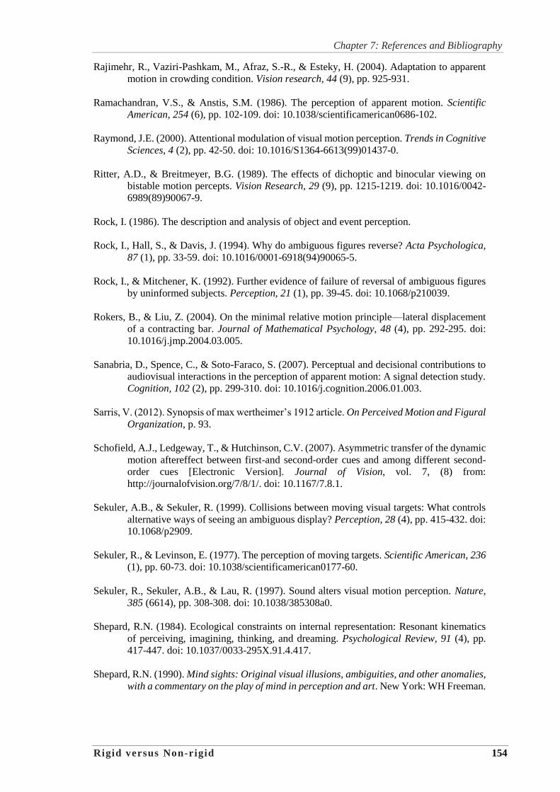
Chapter 7: References and Bibliography
Rigid versus Non-rigid 154
Rajimehr, R., Vaziri-Pashkam, M., Afraz, S.-R., & Esteky, H. (2004). Adaptation to apparent
motion in crowding condition. Vision research, 44 (9), pp. 925-931.
Ramachandran, V.S., & Anstis, S.M. (1986). The perception of apparent motion. Scientific
American, 254 (6), pp. 102-109. doi: 10.1038/scientificamerican0686-102.
Raymond, J.E. (2000). Attentional modulation of visual motion perception. Trends in Cognitive
Sciences, 4 (2), pp. 42-50. doi: 10.1016/S1364-6613(99)01437-0.
Ritter, A.D., & Breitmeyer, B.G. (1989). The effects of dichoptic and binocular viewing on
bistable motion percepts. Vision Research, 29 (9), pp. 1215-1219. doi: 10.1016/0042-
6989(89)90067-9.
Rock, I. (1986). The description and analysis of object and event perception.
Rock, I., Hall, S., & Davis, J. (1994). Why do ambiguous figures reverse? Acta Psychologica,
87 (1), pp. 33-59. doi: 10.1016/0001-6918(94)90065-5.
Rock, I., & Mitchener, K. (1992). Further evidence of failure of reversal of ambiguous figures
by uninformed subjects. Perception, 21 (1), pp. 39-45. doi: 10.1068/p210039.
Rokers, B., & Liu, Z. (2004). On the minimal relative motion principle—lateral displacement
of a contracting bar. Journal of Mathematical Psychology, 48 (4), pp. 292-295. doi:
10.1016/j.jmp.2004.03.005.
Sanabria, D., Spence, C., & Soto-Faraco, S. (2007). Perceptual and decisional contributions to
audiovisual interactions in the perception of apparent motion: A signal detection study.
Cognition, 102 (2), pp. 299-310. doi: 10.1016/j.cognition.2006.01.003.
Sarris, V. (2012). Synopsis of max wertheimer’s 1912 article. On Perceived Motion and Figural
Organization, p. 93.
Schofield, A.J., Ledgeway, T., & Hutchinson, C.V. (2007). Asymmetric transfer of the dynamic
motion aftereffect between first-and second-order cues and among different second-
order cues [Electronic Version]. Journal of Vision, vol. 7, (8) from:
http://journalofvision.org/7/8/1/. doi: 10.1167/7.8.1.
Sekuler, A.B., & Sekuler, R. (1999). Collisions between moving visual targets: What controls
alternative ways of seeing an ambiguous display? Perception, 28 (4), pp. 415-432. doi:
10.1068/p2909.
Sekuler, R., & Levinson, E. (1977). The perception of moving targets. Scientific American, 236
(1), pp. 60-73. doi: 10.1038/scientificamerican0177-60.
Sekuler, R., Sekuler, A.B., & Lau, R. (1997). Sound alters visual motion perception. Nature,
385 (6614), pp. 308-308. doi: 10.1038/385308a0.
Shepard, R.N. (1984). Ecological constraints on internal representation: Resonant kinematics
of perceiving, imagining, thinking, and dreaming. Psychological Review, 91 (4), pp.
417-447. doi: 10.1037/0033-295X.91.4.417.
Shepard, R.N. (1990). Mind sights: Original visual illusions, ambiguities, and other anomalies,
with a commentary on the play of mind in perception and art. New York: WH Freeman.
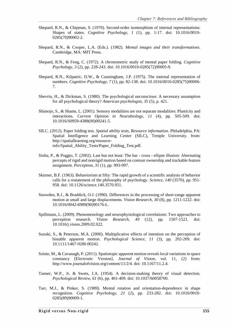
Chapter 7: References and Bibliography
Rigid versus Non-rigid 155
Shepard, R.N., & Chipman, S. (1970). Second-order isomorphism of internal representations:
Shapes of states. Cognitive Psychology, 1 (1), pp. 1-17. doi: 10.1016/0010-
0285(70)90002-2.
Shepard, R.N., & Cooper, L.A. (Eds.). (1982). Mental images and their transformations.
Cambridge, MA: MIT Press.
Shepard, R.N., & Feng, C. (1972). A chronometric study of mental paper folding. Cognitive
Psychology, 3 (2), pp. 228-243. doi: 10.1016/0010-0285(72)90005-9.
Shepard, R.N., Kilpatric, D.W., & Cunningham, J.P. (1975). The internal representation of
numbers. Cognitive Psychology, 7 (1), pp. 82-138. doi: 10.1016/0010-0285(75)90006-
7.
Shevrin, H., & Dickman, S. (1980). The psychological unconscious: A necessary assumption
for all psychological theory? American psychologist, 35 (5), p. 421.
Shimojo, S., & Shams, L. (2001). Sensory modalities are not separate modalities: Plasticity and
interactions. Current Opinion in Neurobiology, 11 (4), pp. 505-509. doi:
10.1016/S0959-4388(00)00241-5.
SILC. (2012). Paper folding test. Spatial ability tests, Resource information. Philadelphia, PA:
Spatial Intelligence and Learning Center (SILC), Temple University. from:
http://spatiallearning.org/resource-
info/Spatial_Ability_Tests/Paper_Folding_Test.pdf.
Sinha, P., & Poggio, T. (2002). Last but not least: The bar - cross - ellipse illusion: Alternating
percepts of rigid and nonrigid motion based on contour ownership and trackable feature
assignment. Perception, 31 (1), pp. 993-997.
Skinner, B.F. (1963). Behaviorism at fifty: The rapid growth of a scientific analysis of behavior
calls for a restatement of the philosophy of psychology. Science, 140 (3570), pp. 951-
958. doi: 10.1126/science.140.3570.951.
Snowden, R.J., & Braddick, O.J. (1990). Differences in the processing of short-range apparent
motion at small and large displacements. Vision Research, 30 (8), pp. 1211-1222. doi:
10.1016/0042-6989(90)90176-L.
Spillmann, L. (2009). Phenomenology and neurophysiological correlations: Two approaches to
perception research. Vision Research, 49 (12), pp. 1507-1521. doi:
10.1016/j.visres.2009.02.022.
Suzuki, S., & Peterson, M.A. (2000). Multiplicative effects of intention on the perception of
bistable apparent motion. Psychological Science, 11 (3), pp. 202-209. doi:
10.1111/1467-9280.00242.
Szinte, M., & Cavanagh, P. (2011). Spatiotopic apparent motion reveals local variations in space
constancy [Electronic Version]. Journal of Vision, vol. 11, (2) from:
http://www.journalofvision.org/content/11/2/4. doi: 10.1167/11.2.4.
Tanner, W.P., Jr, & Swets, J.A. (1954). A decision-making theory of visual detection.
Psychological Review, 61 (6), pp. 401-409. doi: 10.1037/h0058700.
Tarr, M.J., & Pinker, S. (1989). Mental rotation and orientation-dependence in shape
recognition. Cognitive Psychology, 21 (2), pp. 233-282. doi: 10.1016/0010-
0285(89)90009-1.

Chapter 7: References and Bibliography
Rigid versus Non-rigid 156
Taylor, S., & Taylor, M. (2013). Does Alicante have the longest urban geometric illusion in the
world? Perception, 42 (12), pp. 1362-1367. doi: 10.1068/p7549.
Todd, J.T. (1982). Visual information about rigid and nonrigid motion: A geometric analysis.
Journal of Experimental Psychology: Human Perception and Performance, 8 (2), pp.
238-252. doi: 10.1037/0096-1523.8.2.238.
Todd, J.T. (1984). The perception of three-dimensional structure from rigid and nonrigid
motion. Perception & Psychophysics, 36 (2), pp. 97-103. doi: 10.3758/BF03202670.
Todd, J.T., Akerstrom, R.A., Reichel, F.D., & Hayes, W. (1988). Apparent rotation in three-
dimensional space: Effects of temporal, spatial, and structural factors. Perception &
Psychophysics, 43 (2), pp. 179-188. doi: 10.3758/bf03214196.
Todd, J.T., & Norman, J.F. (2003). The visual perception of 3D shape from multiple cues: Are
observers capable of perceiving metric structure? Perception & Psychophysics, 65 (1),
pp. 31-47. doi: 10.3758/BF03194781.
Todorović, D. (1993). Analysis of two-and three-dimensional rigid and nonrigid motions in the
stereokinetic effect. Journal of the Optical Society of America: A - Optics, Image &
Science, 10 (5), pp. 804-826. doi: 10.1364/JOSAA.10.000804.
Tse, P.U. (2006). Neural correlates of transformational apparent motion. Neuroimage, 31 (2),
pp. 766-773. doi: 10.1016/j.neuroimage.2005.12.029.
Tse, P.U., & Logothetis, N.K. (2002). The duration of 3-D form analysis in transformational
apparent motion. Perception & Psychophysics, 64 (2), pp. 244-265. doi:
10.3758/BF03195790.
Tyler, C.W., & Chen, C.-C. (2000). Signal detection theory in the 2afc paradigm: Attention,
channel uncertainty and probability summation. Vision Research, 40 (22), pp. 3121-
3144. doi: 10.1016/S0042-6989(00)00157-7.
Ullman, S. (1983). Maximizing rigidity: The incremental recovery of 3D structure from rigid
and rubbery motion. (Technical Report A.I. Memo No.721). Cambridge, MA:
Massachussetts Institute of Technology, Artificial Intelligence Laboratory.
Vallortigara, G., Bressan, P., & Zanforlin, M. (1986). The Saturn illusion: A new stereokinetic
effect. Vision Research, 26 (5), pp. 811-813. doi: 10.1016/0042-6989(86)90096-9.
Van Ee, R., Noest, A.J., Brascamp, J.W., & van den Berg, A.V. (2006). Attentional control over
either of the two competing percepts of ambiguous stimuli revealed by a two-parameter
analysis: Means do not make the difference. Vision Research, 46 (19), pp. 3129-3141.
doi: 10.1016/j.visres.2006.03.017.
Van Ee, R., Van Dam, L.C.J., & Brouwer, G.J. (2005). Voluntary control and the dynamics of
perceptual bi-stability. Vision Research, 45 (1), pp. 41-55. doi:
10.1016/j.visres.2004.07.030.
Vasquez, R., & Mayora, J. (1991). Kalman filter application to tridimensional rigid body motion
parameter estimation from a sequence of images. S.N. Dwivedi, Verma, A.K. &
Sneckenberger, J.E. (Eds.), CAD/CAM robotics and factories of the future '90. Berlin:
Springer, pp. 412-420. doi: 10.1007/978-3-642-58214-1_63.

Chapter 7: References and Bibliography
Rigid versus Non-rigid 157
Viviani, P., & Aymoz, C. (2001). Colour, form, and movement are not perceived
simultaneously. Vision research, 41(22), 2909-2918.
Wade, N.J. (1994). A selective history of the study of visual motion aftereffects. Perception, 23
(10), pp. 1111-1134.
Walker, A.S., Owsley, C.J., Megaw-Nyce, J., Gibson, E.J., & Bahrick, L.E. (1980). Detection
of elasticity as an invariant property of objects by young infants. Perception, 9 (6), pp.
713-718. doi: 10.1068/p090713.
Webster, M.A. (2002). Adaptation, high-level vision, and the phenomenology of perception
[keynote paper]. Paper presented at Electronic Imaging VII 2002, B.E. Rogowitz &
Pappas, T.N. San Jose, CA: International Society for Optics and Photonics.
Webster, M.A., Werner, J.S., & Field, D.J. (2005). Adaptation and the phenomenology of
perception. C.W.G. Clifford & Rhodes, G. (Eds.), Fitting the mind to the world:
Adaptation and aftereffects in high level vision. Oxford, UK: Oxford University Press,
pp. 241-277. doi: 10.1093/acprof:oso/9780198529699.001.0001.
Weilnhammer, V., Ludwig, K., Sterzer, P., & Hesselmann, G. (2014). Revisiting the Lissajous
figure as a tool to study bistable perception. Vision research, 98, pp. 107-112.
Weiss, Y., & Adelson, E.H. (2000). Adventures with gelatinous ellipses–constraints on models
of human motion analysis. Perception, 29, pp. 543-566. doi: 10.1068/p3032.
Weisstein, E.W. (2003). Poincaré hyperbolic disk.
Welch, R.B., & Warren, D.H. (1980). Immediate perceptual response to intersensory
discrepancy. Psychological Bulletin, 88 (3), pp. 638-667. doi: 10.1037/0033-
2909.88.3.638.
Wertheimer, M. (1912). Experimentelle studien über das sehen von bewegung. JA Barth.
Wertheimer, M., & Spillmann, L. (2012). On perceived motion and figural organization. MIT
Press.
Westheimer, G. (2008). Illusions in the spatial sense of the eye: Geometrical–optical illusions
and the neural representation of space. Vision Research, 48 (20), pp. 2128-2142. doi:
10.1016/j.visres.2008.05.016.
Wickens, T.D. (1989). Multiway contingency table analysis for the social sciences. Hillsdale,
NJ: Lawrence Erlbaum.
Wieland, B.A., & Mefferd, R.B. (1968). Perception of depth in rotating objects: 3. Asymmetry
and velocity as the determinants of the stereokinetic effect. Perceptual and Motor
Skills, 26 (3), pp. 671-681. doi: 10.2466/pms.1968.26.3.671.
Xausa, E., Beghi, L., & Zanforlin, M. (2001). A mathematical model of depth displacement
with a contracting bar. Journal of Mathematical Psychology, 45 (4), pp. 635-655. doi:
10.1006/jmps.2000.1342.
Xausa, E., Beghi, L., & Zanforlin, M. (2006). Stereokinetic phenomena revisited: The
oscillating tilted bar, the swinging gate and the vertical contracting bar. Journal of
Mathematical Psychology, 50 (6), pp. 562-569. doi: 10.1016/j.jmp.2006.03.005.

Chapter 7: References and Bibliography
Rigid versus Non-rigid 158
Zavagno, D. (2005). The phantom illumination illusion. Perception & Psychophysics, 67 (2),
pp. 209-218. doi: 10.3758/BF03206485.
Zhou, K., Luo, H., Zhou, T., Zhuo, Y., & Chen, L. (2010). Topological change disturbs object
continuity in attentive tracking. Proceedings of the National Academy of Sciences, 107
(50), pp. 21920-21924. doi: 10.1073/pnas.1010919108.
Zolfagharifard, E. (2015, 20 August). Mystery of the mona lisa’s smile solved: Second painting
shows how da vinci created an optical illusion to trick viewers, Daily Mail Australia,
Sydney, NSW, Australia. Retrieved: 26/08/2015, from:
http://www.dailymail.co.uk/sciencetech/article-3204079/Mystery-Mona-Lisa-s-smile-
solved-Second-painting-shows-da-Vinci-created-optical-illusion-trick-viewers.html.

Chapter 8: Appendix
Rigid versus Non-rigid 159
CHAPTER 8: APPENDIX
8.1 Participation Information Statement
Discipline of Architecture and
Design Science
Faculty of Architecture, Design and
Planning
ABN 15 211 513 464
CHIEF INVESTIGATOR / SUPERVISOR NAME
A/Prof William Martens
Room 477
G04
The University of Sydney
NSW 2006 AUSTRALIA
Telephone: +61 2 9351 0865
Facsimile: +61 2 9036 9532.
Email: [email protected]
Web: http://www.sydney.edu.au/
Multi-Sensory Integration in Design
PARTICIPANT INFORMATION STATEMENT
(1) What is the study about?
You are invited to participate in a study of how human subjects respond to
complex time-varying stimuli in multi-sensory tasks. Most often the visual and

Chapter 8: Appendix
Rigid versus Non-rigid 160
auditory channels are the major influences on our recognition of motion
percepts. The studies involve a set of visual identification tasks while
observing animated three-dimensional forms. The tasks require participants to
make choices between two alternative responses that identify the type of
visual motion that is perceived while watching a computer-graphic animation
with varying display parameters.
(2) Who is carrying out the study?
The study is being conducted by A. Prof William Martens and Rui (Irene)
Chen, and will form the basis for the degree of PhD at The University of
Sydney under the supervision of A. Prof William Martens.
(3) What does the study involve?
The participants will be asked to fill in one page participant information form
before the experiments and one page feedback and post evaluation form after the
experiments.
The experiments will be run in Room 140 of the Wilkinson Building (G04), which
is the location for the Faculty of Architecture, Design and Planning of the
University of Sydney.
The participants will participate in four sessions of video watching. Each session
contains three subsessions. Each subsession lasts 6 minutes. During each session,
there will be two stages, one is called “adaptation period” and another is called
“test period”. Before the beginning of each stage there will be a brief written
instruction presented on screen to indicate to the participant which task is starting.
There will be five 110-s videos presented continuously with 10-s breaks in between
to allow the participants to rest their eyes and get refocused. While watching the
videos, the participants need to press one of two different keys in order to report
which motion percept is experienced.
Four sessions will be done at different times, if possible on separated days
according to the time available to the participants, and the participants can take
breaks as they like during the sessions.

Chapter 8: Appendix
Rigid versus Non-rigid 161
(4) How much time will the study take?
This study requires the participant to attend four sessions. Each session takes
about 20 minutes to complete, so the total will be about one hour and twenty
minutes.
(5) Can I withdraw from the study?
Participating in this study is completely voluntary - you are not under any
obligation to consent and - if you do consent - you can withdraw at any time
without affecting your relationship with The University of Sydney.
(6) Will anyone else know the results?
All aspects of the study, including individual participant’s results, will be strictly
confidential and only the researchers will have access to information on
participants. A report regarding the results of the study may be submitted for
publication, but individual participants will not be identifiable in such a report.
(7) Will the study benefit me?
We cannot and do not guarantee or promise that you will receive any benefits
from the study.
(8) Can I tell other people about the study?
You can tell other people about the study as you like.

Chapter 8: Appendix
Rigid versus Non-rigid 162
(9) What if I require further information about the study or my involvement in it?
After you have read this information, Rui (Irene) Chen will discuss it with you
further and answer any questions you may have. If you would like to know
more at any stage, please feel free to contact A. Prof William Martens,
Associate Dean (Graduate Research Studies)
[[email protected] | 9114 0865].
(10) What if I have a complaint or any concerns?
Any person with concerns or complaints about the conduct of a research study
can contact The Manager, Human Ethics Administration, University of Sydney
on +61 2 8627 8176 (Telephone); +61 2 8627 8177 (Facsimile) or
[email protected] (Email).
This information sheet is for you to keep

Chapter 8: Appendix
Rigid versus Non-rigid 163
8.2 Participation Information Form

Chapter 8: Appendix
Rigid versus Non-rigid 164
8.3 Participant Consent Form
Discipline of Architecture
and Design Science
Faculty of Architecture,
Design and Planning
ABN 15 211 513 464
CHIEF INVESTIGATOR / SUPERVISOR NAME
A. Prof William Martens
Room 477
G04
The University of Sydney
NSW 2006 AUSTRALIA
Telephone: +61 2 9351 0865
Facsimile: +61 2 9036 9532.
Email: [email protected]
Web: http://www.sydney.edu.au/
PARTICIPANT CONSENT FORM
I, ...........................................................................................[PRINT NAME], give consent
to my participation in the research project

Chapter 8: Appendix
Rigid versus Non-rigid 165
TITLE: Multi-sensory Integration in Design
In giving my consent I acknowledge that:
1. The procedures required for the project and the time involved have been explained to me, and any questions I have about the project have been answered to my satisfaction.
2. I have read the Participant Information Statement and have been given the opportunity to discuss the information and my involvement in the project with the researcher/s.
3. I understand that being in this study is completely voluntary – I am not under any obligation to consent.
4. I understand that my involvement is strictly confidential. I understand that any research data gathered from the results of the study may be published however no
information about me will be used in any way that is identifiable.
5. I understand that I can withdraw from the study at any time, without affecting my
relationship with the researcher(s) or the University of Sydney now or in the future.

Chapter 8: Appendix
Rigid versus Non-rigid 166
6. I understand that I can stop the interview at any time if I do not wish to continue, the video / audio recording will be erased and the information provided will not be included in the study.
I understand that I can stop my participation in the focus group at any time if I do
not wish to continue; however as it is a group discussion it will not be possible to
exclude individual data to that point.
7. I consent to:
Audio-recording YES NO Video-recording YES NO Receiving Feedback YES NO
If you answered YES to the “Receiving Feedback” question, please provide
your details i.e. mailing address, email address.
Feedback Option
Address: _____________________________________________________
_____________________________________________________
Email: _____________________________________________________

Chapter 8: Appendix
Rigid versus Non-rigid 167
............................. ...................................................
Signature
............................. ....................................................
Please PRINT name
..................................................................................
Date
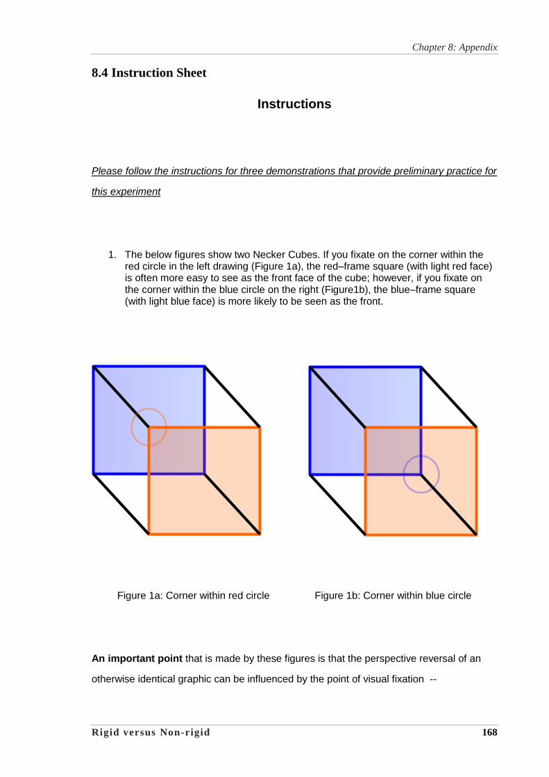
Chapter 8: Appendix
Rigid versus Non-rigid 168
8.4 Instruction Sheet
Instructions
Please follow the instructions for three demonstrations that provide preliminary practice for
this experiment
1. The below figures show two Necker Cubes. If you fixate on the corner within the red circle in the left drawing (Figure 1a), the red–frame square (with light red face) is often more easy to see as the front face of the cube; however, if you fixate on the corner within the blue circle on the right (Figure1b), the blue–frame square (with light blue face) is more likely to be seen as the front.
Figure 1a: Corner within red circle Figure 1b: Corner within blue circle
An important point that is made by these figures is that the perspective reversal of an
otherwise identical graphic can be influenced by the point of visual fixation --
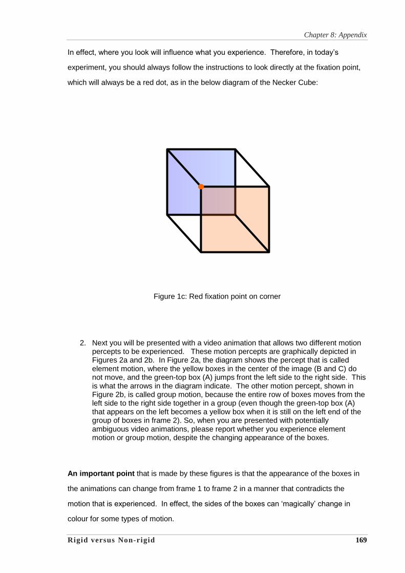
Chapter 8: Appendix
Rigid versus Non-rigid 169
In effect, where you look will influence what you experience. Therefore, in today’s
experiment, you should always follow the instructions to look directly at the fixation point,
which will always be a red dot, as in the below diagram of the Necker Cube:
Figure 1c: Red fixation point on corner
2. Next you will be presented with a video animation that allows two different motion percepts to be experienced. These motion percepts are graphically depicted in Figures 2a and 2b. In Figure 2a, the diagram shows the percept that is called element motion, where the yellow boxes in the center of the image (B and C) do not move, and the green-top box (A) jumps front the left side to the right side. This is what the arrows in the diagram indicate. The other motion percept, shown in Figure 2b, is called group motion, because the entire row of boxes moves from the left side to the right side together in a group (even though the green-top box (A) that appears on the left becomes a yellow box when it is still on the left end of the group of boxes in frame 2). So, when you are presented with potentially ambiguous video animations, please report whether you experience element motion or group motion, despite the changing appearance of the boxes.
An important point that is made by these figures is that the appearance of the boxes in
the animations can change from frame 1 to frame 2 in a manner that contradicts the
motion that is experienced. In effect, the sides of the boxes can ‘magically’ change in
colour for some types of motion.
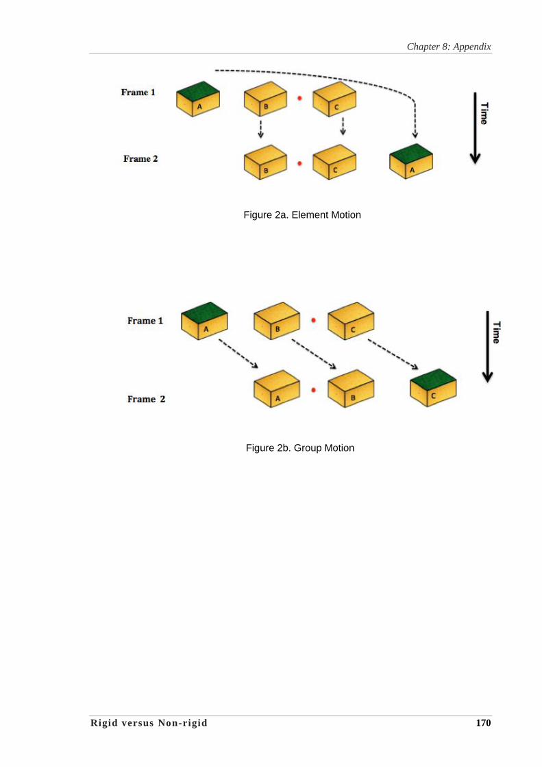
Chapter 8: Appendix
Rigid versus Non-rigid 170
Figure 2a. Element Motion
Figure 2b. Group Motion
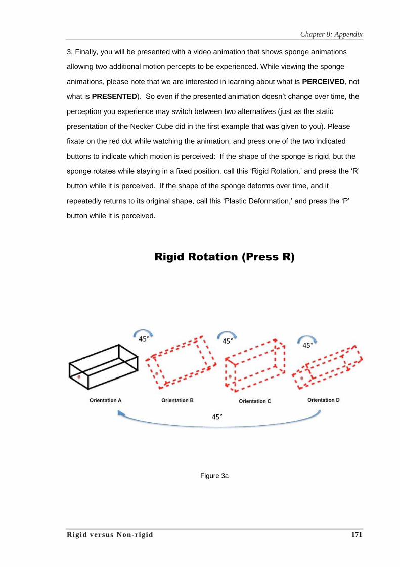
Chapter 8: Appendix
Rigid versus Non-rigid 171
3. Finally, you will be presented with a video animation that shows sponge animations
allowing two additional motion percepts to be experienced. While viewing the sponge
animations, please note that we are interested in learning about what is PERCEIVED, not
what is PRESENTED). So even if the presented animation doesn’t change over time, the
perception you experience may switch between two alternatives (just as the static
presentation of the Necker Cube did in the first example that was given to you). Please
fixate on the red dot while watching the animation, and press one of the two indicated
buttons to indicate which motion is perceived: If the shape of the sponge is rigid, but the
sponge rotates while staying in a fixed position, call this ‘Rigid Rotation,’ and press the ‘R’
button while it is perceived. If the shape of the sponge deforms over time, and it
repeatedly returns to its original shape, call this ‘Plastic Deformation,’ and press the ‘P’
button while it is perceived.
Figure 3a
Rigid Rotation (Press R)
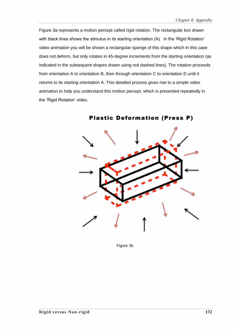
Chapter 8: Appendix
Rigid versus Non-rigid 172
Figure 3a represents a motion percept called rigid rotation. The rectangular box drawn
with black lines shows the stimulus in its starting orientation (A). In the ‘Rigid Rotation’
video animation you will be shown a rectangular sponge of this shape which in this case
does not deform, but only rotates in 45-degree increments from the starting orientation (as
indicated in the subsequent shapes drawn using red dashed lines). The rotation proceeds
from orientation A to orientation B, then through orientation C to orientation D until it
returns to its starting orientation A. This detailed process gives rise to a simple video
animation to help you understand this motion percept, which is presented repeatedly in
the ‘Rigid Rotation’ video.
Figure 3b.
Chapter 8: Appendix
Rigid versus Non-rigid 173
Figure 3b represents a motion percept called plastic deformation. The black lines indicate
a deformable rectangular sponge, which after being squeezed or squashed according to
the forces indicated by the black arrows, takes on the new shape that is drawn using red
dashed lines. It can be restored to its original shape according to the forces drawn with
the red arrows. This detailed process gives rise to a simple video animation to help you
understand this motion percept, which is presented repeatedly in the ‘Plastic Deformation’
video.

Chapter 8: Appendix
Rigid versus Non-rigid 174
8.5 Feedback and Post-evaluation
Discipline of Architecture and
Design Science
Faculty of Architecture, Design
and Planning
ABN 15 211 513 464
CHIEF INVESTIGATOR / SUPERVISOR NAME
A. Prof William Martens
Room 477
G04
The University of Sydney
NSW 2006 AUSTRALIA
Telephone: +61 2 9351 0865
Facsimile: +61 2 9036 9532.
Email: [email protected]
Web: http://www.sydney.edu.au/
Feedback and Post-evaluation
Please indicate your response to the following four questions by drawing a
vertical line somewhere along the horizontal line below the written labels.
1. How much (if any) any eye strain or fatigue did you experience during the experiment?
None a little not too much too much way too
much
+------------------------+--------------------------+--------------------------+-------------------------+

Chapter 8: Appendix
Rigid versus Non-rigid 175
2. How much discomfort did you experience during the experiment due to the lighting in the room?
None a little not too much too much way too
much
+------------------------+--------------------------+--------------------------+-------------------------+
3. How much difficulty did you have disregarding the colour on the object surface in reporting on your motion perception?
None a little not too much too much way too
much
+------------------------+--------------------------+--------------------------+-------------------------+
4. How much difficulty did you have maintaining your focus on the fixation point while reporting on your motion perception?
None a little not too much too much way too
much
+------------------------+--------------------------+--------------------------+----------------------+

Chapter 8: Appendix
Rigid versus Non-rigid 176
8.6 Hierarchical Loglinear Analysis of Combined Data in Output 4way
Table
Hierarchical Loglinear Analysis of Combined Data
(i.e., both 2-Frame and 4-Frame Results)
Notes
Output Created 19-AUG-2014 11:19:26
Comments
Input Active Dataset DataSet3
Filter <none>
Weight Count
Split File <none>
N of Rows in Working Data File 48
Missing Value Handling
Definition of Missing
User-defined missing
values are treated as
missing.
Cases Used
Statistics are based on
all cases with valid data
for all variables in the model.
Syntax
HILOGLINEAR F(1 2)
R(1 2) A(1 2) I(1 6)
/CWEIGHT=Count
/METHOD=BACKWARD
/CRITERIA MAXSTEPS(10)
P(.05) ITERATION(20)
DELTA(.5)
/PRINT=FREQ RESID
/DESIGN.
Resources Processor Time 00:00:00.06
Elapsed Time 00:00:00.00
Convergence Information
Generating Class F*R*A*I
Convergence Criterion 181.476

Chapter 8: Appendix
Rigid versus Non-rigid 177
Backward Elimination Statistics
Step
Summary
Stepa Effects Chi-Squarec df Sig. Number of
Iterations
0 Generating Classb F*R*A*I .000 0 .
Deleted Effect 1 F*R*A*I 2.154 5 .827 2
1
Generating Classb F*R*A, F*R*I,
F*A*I, R*A*I
2.154 5 .827
Deleted Effect 1 F*R*A 57.180 1 .000 2
2 F*R*I 2.040 5 .844 2
3 F*A*I .713 5 .982 2
4 R*A*I 1.993 5 .850 2
2 Generating Classb
F*R*A, F*R*I,
R*A*I
2.868 10 .984
Deleted Effect 1 F*R*A 56.533 1 .000 2
K-Way and Higher-Order Effects
K df Likelihood Ratio Pearson Number of Iterations
Chi-Square Sig. Chi-Square Sig.
K-way and Higher Order Effectsa
1 47 1928.494 .000 1834.400 .000 0
2 39 525.429 .000 516.409 .000 2
3 21 63.518 .000 63.241 .000 2
4 5 2.154 .827 2.156 .827 2
K-way Effectsb
1 8 1403.065 .000 1317.991 .000 0
2 18 461.911 .000 453.167 .000 0
3 16 61.363 .000 61.085 .000 0
4 5 2.154 .827 2.156 .827 0
a. Tests that k-way and higher order effects are zero.
b. Tests that k-way effects are zero.
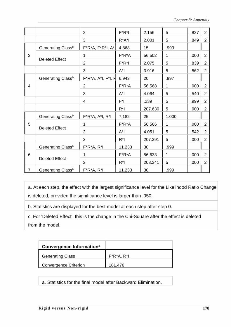
Chapter 8: Appendix
Rigid versus Non-rigid 178
2 F*R*I 2.156 5 .827 2
3 R*A*I 2.001 5 .849 2
3
Generating Classb F*R*A, F*R*I, A*I 4.868 15 .993
Deleted Effect 1 F*R*A 56.502 1 .000 2
2 F*R*I 2.075 5 .839 2
3 A*I 3.916 5 .562 2
4
Generating Classb F*R*A, A*I, F*I, R*I 6.943 20 .997
2 F*R*A 56.568 1 .000 2
3 A*I 4.064 5 .540 2
4 F*I .239 5 .999 2
R*I 207.630 5 .000 2
5
Generating Classb F*R*A, A*I, R*I 7.182 25 1.000
Deleted Effect 1 F*R*A 56.566 1 .000 2
2 A*I 4.051 5 .542 2
3 R*I 207.391 5 .000 2
6
Generating Classb F*R*A, R*I 11.233 30 .999
Deleted Effect 1 F*R*A 56.633 1 .000 2
2 R*I 203.341 5 .000 2
7 Generating Classb F*R*A, R*I 11.233 30 .999
a. At each step, the effect with the largest significance level for the Likelihood Ratio Change
is deleted, provided the significance level is larger than .050.
b. Statistics are displayed for the best model at each step after step 0.
c. For 'Deleted Effect', this is the change in the Chi-Square after the effect is deleted
from the model.
Convergence Informationa
Generating Class F*R*A, R*I
Convergence Criterion 181.476
a. Statistics for the final model after Backward Elimination.

Chapter 8: Appendix
Rigid versus Non-rigid 179
8.7 Thesis Website
Please visit: http://easyrace.wixsite.com/icsponge