1

Forthcoming (with minor changes) in:

ECONOMIC POLICY (Vol. 81), January 2015

What drives the German current account?

And how does it affect other EU member states? (*)

Robert Kollmann (ECARES, Université Libre de Bruxelles; CEPR; CAMA),

Marco Ratto (JRC, EU Commission),

Werner Roeger (DG-ECFIN, EU Commission),

Jan in’t Veld (DG-ECFIN, EU Commission),

Lukas Vogel (DG-ECFIN, EU Commission)

April 24, 2014

We estimate a three-country model using 1995-2013 data for Germany, the Rest of the Euro

Area (REA) and the Rest of the World (ROW) to analyze the determinants of Germany’s

current account surplus after the launch of the Euro. The most important factors driving the

German surplus were positive shocks to the German saving rate and to ROW demand for

German exports, as well as German labour market reforms and other positive German

aggregate supply shocks. The convergence of REA interest rates to German rates due to the

creation of the Euro only had a modest effect on the German current account and on German

real activity. The key shocks that drove the rise in the German current account tended to

worsen the REA trade balance, but had a weak effect on REA real activity. Our analysis

suggests these driving factors are likely to be slowly eroded, leading to a very gradual

reduction of the German current account surplus. An expansion in German government

consumption and investment would raise German GDP and reduce the current account

surplus, but the effects on the surplus are likely to be weak.

JEL Classification: F4, F3, F21, E3

Keywords: Current Account, intra-European imbalances, monetary union, Eurozone crisis,

estimated DSGE model.

(*)

This version of the paper was presented at the 59th

Panel Meeting of Economic Policy

(CEPR, CES, PSE/ENS) hosted by the Central Bank of Turkey, April 25-26, 2014.

Economic Policy does not allow web posting of revised (post-conference) versions. Please

e-mail R. Kollmann to receive the final paper accepted for publication (revisions are

only stylistic and very minor, all substantive results can be found in version here).

The views expressed in this paper are those of the authors and should not be attributed to the

European Commission. We are very grateful to Refet Gürkaynak, Marcel Fratzscher, Gernot

Müller, Jeromin Zettelmeyer and to three anonymous referees for detailed and constructive

comments. We also thank Caterina Mendicino and Gábor Pellényi for useful discussions.

Helpful comments were also received from Tobias Cwik, Maria Demertzis, Mercedes De

Miguel Cabeza, Jakob Friis, Bettina Kromen and from workshop participants at the EEA,

VfS and DYNARE conferences, and at the ECB, National Bank of Hungary, National Bank

of Poland, Swiss National Bank and LUISS (Rome). Research support from Jukka

Heikkonen, Christoph Maier and Beatrice Pataracchia is also gratefully acknowledged.

Corresponding author: Robert Kollmann, ECARES, CP 114, Université Libre de Bruxelles,

50. Av. Franklin Roosevelt, B-1050 Brussels, Belgium.

E-mail addresses: robert_kollmann@yahoo.com, marco.ratto@jrc.ec.europa.eu,

werner.roeger@ec.europa.eu, jan.intveld@ec.europa.eu, lukas.vogel@ec.europa.eu

2

1. Introduction

Germany experienced a spectacular current account (CA) reversal, after the launch of the

Euro (1999). In the 1990s, the German current account was in deficit, but close to balance—

however, in the early 2000s, the current account shifted to steadily increasing surpluses, vis-

à-vis both the rest of the Euro Area (REA) and the rest of the world (ROW).1 During the

financial crisis, German capital flows to the REA fell abruptly, but the overall German

current account surplus bounced back rapidly and reached record levels--185 bill. EUR in

2012, i.e. 7% of German GDP--due inter alia to a rise in the surplus vis-à-vis Asia. As a

result, Germany has become one of the major surplus countries in the world.

These developments are currently at the heart of heated debates about the role of the

German surplus and of intra-Euro Area external imbalances for the crisis and the slow

recovery in Europe (see Lane (2012), Chen, Milesi-Ferretti and Tressel (2012) and Hobza

and Zeugner (2013) for discussions of intra-EA imbalances). On October 30, 2013, the U.S.

Treasury sharply criticized Germany’s external surplus: ‘Germany’s anemic pace of domestic

demand growth and dependence on exports have hampered rebalancing at a time when many

other euro-area countries have been under severe pressure to curb demand and compress

imports in order to promote adjustment. The net result has been a deflationary bias for the

euro area, as well as for the world economy’ (U.S. Treasury (2013), p.3). In the Treasury’s

view: ‘To ease the adjustment process within the euro area, countries with large and

persistent surpluses need to take action to boost domestic demand growth and shrink their

surpluses’ (p.25). The German Government swiftly rejected the US criticism. The German

Economics Ministry stated that ‘The Trade surpluses reflect the strong competitiveness of the

German economy and the international demand for quality products from Germany’ (Wall

Street Journal, October 31, 2013); the German Finance Ministry argued that the German

current account surplus was ‘no cause for concern, neither for Germany, nor for the

Eurozone, or the global economy,’ and that ‘On the contrary, the innovative German

economy contributes significantly to global growth through exports and the import of

components for finished products’ (Financial Times, October 31, 2013).

The IMF has likewise repeatedly expressed concerns about the German external

surplus, and argued that ‘stronger and more balanced growth in Germany is critical to a

lasting recovery in the euro area and global rebalancing’ (IMF Executive Board, August 6,

2013a). By contrast to the U.S. Treasury, the IMF’s policy advice centers on structural

reforms in the German economy, such as measures to increase the productivity of the service

sector and labour force participation. The European Commission too advocates supply side

policies for Germany that ‘strengthen domestic sources of potential growth against the

background of unfavourable demographic prospects’ (European Commission, Alert

Mechanism Report 2014, November 2013). In November 2013, the persistent German current

account surplus triggered an ‘In-Depth Review’ by the EU Commission, under the

Commission’s ‘Macroeconomic Imbalances Procedure’. The review (whose results were

published in March 2014) concluded that the German surplus constitutes an ‘imbalance’ (see

Box on the Macroeconomic Imbalances Procedure below).2

The goal of this paper is to shed light on these policy issues, using a state-of-the-art

macroeconomic model. Economic theory suggests that a country’s current account reflects

domestic and foreign macroeconomic and financial shocks, and the structural features of the

domestic and foreign economies. An understanding of those shocks and structural properties

is thus crucial for positive and normative evaluations of the current account, and for policy

1 Throughout this paper, the term ‘Euro Area’ (EA) refers to the 17 countries that were members of the Euro

Area in 2013. REA is an aggregate of the EA less Germany. 2 The German external surplus has also widely been discussed in the media. Prominent critics of the surplus

include Krugman (2013) and Wolf (2013).

3

advice (Obstfeld and Rogoff (1996), Obstfeld (2012), Kollmann (1998, 2001, 2004)). This

underscores the importance of analyzing the current account using a structural model that

captures the relevant shocks, and their transmission to the macroeconomy.

This paper therefore studies the German current account using an estimated Dynamic

Stochastic General Equilibrium (DSGE) model with three countries: Germany, the REA and

the ROW. The model is estimated using quarterly data for the period 1995q1-2013q2. The

model assumes a rich set of demand and supply shocks in goods, labour and asset markets,

and it allows for nominal and real rigidities, and financial frictions. 3

Several hypotheses about the causes of Germany's external surplus have been debated

in the policy and academic literature. Those causes have mostly been discussed separately,

although in reality these drivers can operate jointly. Our estimated model allows us to recover

the shocks that drive the German external balance—and, hence, we can determine what

shocks mattered most, and when. The model also allows us to assess what policy measures

might best be suited for changing the German external surplus.

We devote particular attention to the following potential causes of the German

external surplus: (i) In the run-up to the Euro (1995-1998), REA interest rates converged to

German rates, an indication that the Euro led to greater financial integration in Europe; it has

frequently been argued (e.g., Sinn (2010) and Hale and Obstfeld (2013)) that greater financial

integration triggered capital flows from Germany to the REA. (ii) A second widely discussed

factor was the strong growth in emerging economies during the past two decades--German

exports may have benefited particularly from the rising demand for investment goods by

emerging economies, given German’s specialization in the production of those goods; strong

growth in emerging economies may have also have added to intra-EA imbalances by

increasing competition for exports from the EMU periphery (e.g., Chen et al. (2012)). (iii)

The German labour market liberalization during the period 2002-2005 (which was driven i.a.

by the growth of outsourcing by German firms to low wage countries, notably in Eastern

Europe) has often been viewed as factor that raised German labour supply, and restrained

German wage growth, thereby boosting German competitiveness (e.g., Dustmann et al.

(2014)). (iv) Finally, it has been argued that depressed German domestic demand (as pointed

out above), and thus a high saving rate, are key drivers of the German surplus; high saving

may partly reflect German households’ concerns about rapid population ageing, following

pension reforms (2001-2004) that markedly lowered state-funded pensions, and created tax

incentives for private retirement saving (Deutsche Bundesbank (2011), Huefner and Koske

(2010)). Fiscal consolidation in Germany after the financial crisis may also have contributed

to weak domestic demand (Lagarde (2012), IMF (2013b), in 't Veld (2013)).

Our empirical results suggest that all of these factors played a role in driving the

German external surplus, but that their quantitative importance and timing differed markedly.

Mono-causal explanations of the German surplus are, thus, insufficient: the surplus reflects a

succession of distinct shocks.

According to the estimated model, greater financial integration (narrowing of the

REA-German interest rate spread) had a positive effect on aggregate demand in the REA,

which boosted REA and German GDP and raised the German current account. However,

quantitatively, these effects are rather modest, and they operated mainly during the late 1990s

and early 2000s; thus, REA-German interest rate convergence cannot explain the persistence

of the rise of the German external surplus. We find that strong ROW growth contributed

positively to German and REA GDP and net export—the effect of ROW growth was stronger

than that of interest rate convergence, and it mainly affected the German external balance

3Earlier applications of similar models can be found in in’t Veld, Raciborski, Ratto and Roeger (2011),

Kollmann, Roeger and in’t Veld (2013) and Kollmann, Ratto, Roeger and in’t Veld (2013).

4

between the early 2000s and the global recession. German labour market reforms had a

marked effect on German GDP and the German current account, after 2007; these reforms

also had a positive, but much weaker, effect on REA GDP (due to stronger German demand

for REA exports), and a weak negative effect on REA net exports. According to our

estimates, positive shocks to German private saving strongly depressed aggregate demand in

Germany after the mid-2000s and lowered German GDP, while raising the German current

account; these shocks also stimulated aggregate demand in the REA (due to a fall in interest

rates).

All in all, the key shocks that drove German real activity and the German current

account only had a minor effect on real activity and inflation in the REA. In other terms, real

activity in the REA was largely driven by domestic factors rather than by German economic

conditions. The key supply and demand shocks that kept the German surplus at a high level

likewise only had a weak effect on inflation in the REA. The model also allows us to make

predictions about the future path of the German external balance. The rise in the interest rate

spread between the REA and Germany since the sovereign debt crisis, and pressure toward

labour market reform in the REA suggest a gradual reduction of the German current account

surplus. Also the effects of labour market reforms enacted in Germany during the early 2000s

are likely to be gradually eroded by higher German real wage growth, signs of which are

already becoming visible (e.g. the new German Federal Government elected in the Fall of

2013 plans to introduce a minimum wage law). The German fiscal stance is also likely to

become less restrictive, allowing a reversal of the trend decline in public investment. And

given low interest rates in Germany, residential investment is also likely to pick up.

What light do these results shed on the policy debate about the German surplus? Our

findings are consistent with the view that adverse shocks to domestic demand were key

drivers of the surplus, especially after the mid-2000s. Our analysis also supports the official

German view that strong external demand and German competitiveness gains (wage

moderation and technological improvements) were important sources of the German external

surplus. However, strong external demand and German competitiveness gains explain, at

most 1/3 to 1/2 of the surplus; strong external demand mattered mainly before the financial

crisis, while wage restraint induced by labour market reforms contributed to the German

surplus after the mid-2000s. The relative role of these factors has thus varied greatly across

time. Positive shocks to the German saving rate have been especially important since the

mid-2000s.

The view that German labour market reforms represented ‘wage dumping’ at the

expense of foreign economies (e.g., Flassbeck (2012)) is not consistent with our estimation

results, due to the very modest effects of the reforms on real activity in the rest of the Euro

Area.

Our analysis suggests that structural reforms to raise productivity and labour supply in

the rest of the Euro Area would benefit the REA economies, and also lower the German

external surplus. Boosting German government consumption would only have a modest

stimulative effect on German GDP, on the German current account, and on REA GDP.

Increases in German government investment would boost German output much more, but

would lead to an even more modest fall in the current account. Measures that raise German

wages would lower German GDP and the German current account. Additional structural

reforms to boost German aggregate supply would tend to further raise the German external

surplus, in the short and medium term--which contrasts with the often-held view that such

measures would lower the German surplus (see above).

The present paper is related to a vast empirical and theoretical literature that has

studied ‘sudden stops,’ i.e. episodes in which large and persistent current account deficits

suddenly come to an end, due to a drop in foreign capital inflows (e.g. Milesi-Ferretti and

5

Razin (1998), Adalet and Eichengreen (2007), Mendoza (2010), Fornaro (2013)). By

contrast, the paper here analyzes a rapid and persistent current account ‘surge’ that follows a

prolonged period of current account balance.

In terms of related academic literature, it can be noted that several papers have

analyzed the dynamics of the current account using two-country DSGE models (e.g.,

Kollmann (1998), Erceg et al. (2006)); by contrast to the paper here, that literature has

typically used calibrated (not estimated) models, and it has abstracted from housing markets

and the key financial frictions considered in the present model. Jacob and Peersman (2013)

study the determinants of the US current account deficit, using an estimated two-country

model; that model too abstracts from housing and financial frictions. The paper here also

differs from these studies, by considering a three-country set-up. A key advantage of that set-

up is that a German trade surplus does not necessarily lead to a trade deficit of the same size

in other EA countries (as would be the case in a standard two-country model). Empirically,

the REA trade balance is not a perfect mirror image of the German TB. Also, the REA is a

less important trading partner for Germany than the ROW; the share of exports to the REA in

German exports fell from 46% in 1995 to 36% in 2012, while the share of the EA in German

imports fell from 47% to 37%.

Section 2 describes Germany’s external balance and macroeconomic conditions in

Germany, the REA and the ROW, during the period 1991-2012. Section 3 provides a brief

overview of our model. Section 4 presents the model estimates. Section 5 concludes.

Box on Macroeconomic Imbalances Procedure:

Drawing lessons from the financial and economic crisis, the European Commission has strengthened

macroeconomic surveillance by introducing the Macroeconomic Imbalances Procedure (MIP) in

2011. The aim of the MIP is to identify potential risks to macroeconomic stability at an early stage

and to ensure that Member States adopt appropriate policy responses to prevent harmful imbalances

and correct those that have already built up.

EU Regulation No 1176/2011 characterizes a macroeconomic imbalance as "any trend giving rise to

macroeconomic developments which are adversely affecting, or have the potential adversely to affect,

the proper functioning of the economy of a Member State or of the Economic and Monetary Union, or

of the Union as a whole." Excessive imbalances are defined as "severe imbalances that jeopardize or

risk jeopardizing the proper functioning" of EMU.

The MIP adopts a graduated approach. The first step is a screening for potential imbalances against

a scoreboard of eleven indicators, comprising the current account balance, the net international

investment position, the real effective exchange rate, nominal unit labour costs, the export market

share, the unemployment rate, house price developments, private sector credit, private sector debt,

government debt, and financial sector liabilities. The MIP scoreboard establishes threshold values for

each indicator. The result of the screening by the European Commission is published in the annual

Alert Mechanism Report (AMR). The violation of one or several threshold values provides an early

warning and indicates the need for further analysis by the European Commission in the form of an In-

Depth Review (IDR). On the basis of the IDR, the Commission determines whether imbalances, and

excessive imbalances, exist.

If the European Commission concludes that excessive imbalances exist in a Member State, it may, in a

third step, recommend to the European Council that the Member State concerned draw up a

corrective action plan. After adoption of the recommendation by the Council, the European

Commission and the European Council monitor its implementation. Repeated failure to take action

can, in a fourth step, lead to financial sanctions: the European Commission can propose to the

European Council to levy a fine for not taking action. The European Council decides by reverse

qualified majority vote, i.e. sanctions are approved unless overturned by a qualified majority of

Member States.

6

The scoreboard-based AMR of November 2013 concluded that IDRs were warranted for 16 Member

States, including Germany. The IDR for Germany has been motivated in particular by the breach of

the current account threshold. The latter issues an alert whenever the three-year average of the

current account balance as a percentage of GDP exceeds 6% or falls below -4%.

The current account indicator has upper and lower bounds because both large surpluses and large

deficits can be the result of inefficiencies and adversely affect the proper functioning of monetary

union. The threshold values establish tighter limits on the deficit side. This derives from the view that

current account deficits pose greater risk for macroeconomic stability than current account surpluses.

In particular, large and growing deficits are associated with risks of sudden stops and financial

contagion (European Commission (2012b)).

The European Commission published its IDR on Germany on March 5, 2014. It concluded that

Germany is experiencing macroeconomic imbalances, which require monitoring and policy action.

According to the IDR, the large and persistent external surplus "stems primarily from a lack of

domestic demand, which in turn poses risks to the growth potential of the German economy."

(European Commission (2014), p.107). The European Commission argues it would therefore be

important to identify and implement measures that help strengthen demand and the economy's growth

potential. The report discusses measures to address the backlog in public investment, to further

reduce disincentives to work, to improve the business environment in order to support private

investment, and to ensure that the banking sector has sufficient loss absorption capacity to withstand

economic and financial shocks. The IDR did not include an explicit quantitative discussion of

spillovers.

The Commission will put forward country specific recommendations to deal with the imbalance by

early June 2014, for consideration by the European Council.

2. Macroeconomic conditions and the German external account, 1991-2012

Germany’s current account balance (CA) and trade balance (TB) in the period 1991-2012 are

plotted in Figure 1.a. The dynamics of the CA is closely linked to that of the TB (i.e. to net

exports). After close-to-balance positions in the 1990s, the TB and the CA have been in

persistent surplus since the early 2000s. The German TB and CA surpluses peaked at about

7% of GDP in 2007, receded to about 5%-6% in the global recession of 2008-9, and reached

6%-7% of GDP in 2012; these persistent surpluses have led to a substantial positive

international investment position, that amounted to 35% of German GDP in 2011 (Figure

1.b). The balance on incomes and transfers shows a persistent increase (from about -2% to

+1% of GDP) starting in 2003, but the overwhelming part of the rise in the German current

account since the early 2000s is linked to the rise in net exports.4

Saving, investment and the German external balance

The current account equals the difference between gross national saving (S) and gross

national investment (I): CA=S-I. Figure 1.c plots German saving and investment, in % of

GDP (Y). (All ratios of variables to GDP discussed in the following paragraphs are ratios of

nominal variables.) The German investment rate (I/Y) rate had a slight downward trend in the

1990s; it fell markedly during the early 2000s, and thereafter fluctuated without trend around

a mean value that was about 4 ppt (percentage points) below the mean investment rate

observed in the 1990s.5 The German saving rate (S/Y) closely tracked I/Y until the early

2000s, but rose markedly and persistently during the 2000s (by close to 4ppt between 2000

4 The rise in the German net incomes and transfers balance is solely driven by the rise in net financial income

that resulted from the rise in the German net international investment position. Net international transfers are

very stable across time, and represent about -1.4% of German GDP throughout the sample period. The net

income balance was slightly negative during the second half of the 1990s. Thereafter, net income rose steadily,

due to the rise in the German net international investment positions, and reached 2.4% of German GDP in 2012.

Net financial income accounts for the lion share of net income (net employee income is negligible). 5 See DIW (2013) for a detailed analysis of the decline in the German investment rate.

7

and 2012). This divergence between saving and investment rates accounts for the sharp and

persistent rise of the German current account in the early 2000s. Figure 1.d shows that the

persistent rise in the German current account is accounted for by a persistent rise in the

private sector saving-investment gap. The German fiscal surplus (government S-I) fluctuated

cyclically, but was essentially trendless (as a fraction of GDP), and thus did not contribute to

the persistent rise in the German current account.

Figure 1.e shows the contributions of private consumption (C) and government

consumption (G), and of investment (I) to German net exports: NX=(Y-C-G)-I. The (C+G)/Y

ratio has, essentially, been trend-less throughout the sample period, but exhibited some

marked transient changes (see Fig. 1.f). Saving, S, equals Y-C-G plus net incomes and

transfers from the rest of the world. The fact that S/Y rose after 2002, while (Y-C-G)/Y has

been trendless reflects thus the persistent rise in the balance on income and transfers.

Figure 1.g plots ratios of German exports and imports (of goods and services) to

GDP. Both ratios have steadily trended upward, doubling during the past two decades. The

two ratios have mostly moved in tandem—except in the period 2001-03, when the

imports/GDP ratio fell, while the exports/GDP ratio continued to grow.

Figure 1.h plots German net exports to the REA, total REA net imports, overall

German net exports, and Euro Area (EA) net exports (these variables are reported in % of EA

GDP). German net exports are highly positively correlated with REA net imports. However,

the REA trade balance is not a perfect mirror image of the German TB. E.g., the German

trade balance surplus remained sizable after the financial crisis, while REA net imports fell

sharply. The rise in German net exports to the REA only accounts for about one half of the

deterioration of the overall REA trade balance between the 1990s and 2008. The EA as a

whole ran a trade balance surplus throughout the sample period. During the sample period,

the share of the (fast-growing) ROW in total German foreign trade has risen steadily. The

share of exports to the REA in German exports fell from 46% in 1995 to 36% in 2012, while

the share of the EA in German imports fell from 47% to 37%.

Real activity in Germany and in German export markets

Figures 2.a plots volume series of GDP, private consumption, government purchases and

investment for Germany (compared to the base year 1995). German private consumption

growth in real terms has been lower than real GDP growth since the mid-2000. (The stability

of the ratio of nominal consumption to nominal GDP documented above reflects a gradual

rise in the ratio of the German CPI to the German GDP deflator.) More strikingly, however,

real investment demand has only had a very weak positive trend between 1995 and 2012, but

experienced large temporary ups and downs.

Figure 2.b plots year-on-year (YoY) growth rates of real GDP in Germany, the REA

and the ROW. (ROW output is aggregate real GDP in 40 industrialized and emerging

economies, including EU members who are not EA members; see Appendix.) Output growth

fluctuations have been highly synchronized across these countries/regions. However, German

real GDP grew noticeably less than REA and ROW GDP during 1995-2005. The gap in

growth rates was especially sizable in 2002-2005. During that period Germany was

sometimes referred to as the ‘laggard of Europe’ (Sinn, 2003). Since 2006, German GDP has

grown faster than REA GDP, except during the Great Recession of 2009. ROW growth has

markedly exceeded REA growth since the early 2000s.

REA-German interest rate convergence

The creation of the Euro eliminated exchange rate risk, and reduced financial transaction

costs across member countries. The date of the launch of the Euro (1.1.1999) was announced

by the European Council in December 1995. Until 1995, the nominal interest rate on short

term government debt was markedly higher in the REA than in Germany; see Figure 3.a

8

(mean REA-German interest rate spread: 2.3% p.a. in 1991-1995). The German nominal

interest rate had a flat trend between 1995 and 1999, while the REA nominal rate fell rapidly,

and thus converged to the German rate. The REA-German nominal interest rate spread was

(essentially) zero when the Euro was launched in 1999. Between 1999 and the financial

crisis, the interest rate spread remained very small; a positive spread emerged again after the

eruption of the sovereign debt crises in some REA countries (2010).

Exchange rates and inflation

Due to strong domestic demand (fuelled i.a. by expansionary fiscal policy) the Deutsche

Mark (DM) appreciated against REA and ROW currencies between German Reunification

(1990) and 1995. The DM then depreciated against the REA until the launch of the Euro, but

that depreciation only partly undid the strong post-Reunification appreciation (see Figure

3.c).

It has been argued that Germany entered EMU at an overvalued exchange rate--and

that hence low wage and price growth was needed to re-establish German competitiveness

(internal devaluation) after the launch of the Euro (e.g., Louanges (2005) and Carton and

Hervé (2012)). The path of the real exchange rate of Germany plotted in Figure 3.d is

consistent with that view. After the launch of the Euro, German real depreciation vis-à-vis

the REA has continued via lower German inflation (see Figure 3.b): the average annual

growth rate of the GDP deflator after 1999 was 0.75% in Germany, and 2.49% in the REA.

The nominal (effective) exchange rate of Germany against the ROW depreciated much more

strongly than the German-REA exchange rate, between 1995 and 2001; the German-ROW

exchange rate then appreciated, by more than 70%, until 2008. Since the financial crisis, the

external value of the Euro has fluctuated widely, around a slight downward trend (Fig. 3.d.).

Due to nominal interest rate convergence, the lower German inflation implied that the

German real interest rate was higher than the REA real interest during the first 10 years of

the Euro. The financial crisis led to a rise in German inflation, and to a sharp reduction in

REA inflation.

Labour market reforms

As a response to stagnant real activity in the early 2000s, the German government

implemented a far-reaching labour market deregulation in 2003-05 (‘Hartz’ reforms) that

included a reduction in unemployment benefits and measures such as a re-organization of

labour placement and of job training schemes to improve job matching. Fig. 4.d plots the

German average unemployment benefit ratio (ratio of unemployment benefit to wage rate).

The benefit ratio fell permanently in 2004-05, from 62% to 53%. German labour market

reforms arguably weakened the bargaining power of German trade unions. The fraction of

wage earners who are union members fell steadily from 29% in 1995 to 18% in 2011 (OECD

(2013)). It has been argued that the growth of outsourcing by German firms to low wage

countries, notably in Eastern Europe, also reduced German trade union power (Dustmann et

al. (2014)). These developments may have contributed to the very low growth of wages and

of unit labour costs in Germany and thus to low German inflation (see below). These factors

raised the competitiveness of German exporters, relative to the rest of the EA.

Wages and unit labour cost

Nominal wage growth has been markedly lower in Germany than in the aggregate EA during

most of the Euro-era (see Fig. 4.a). Between 2002 and 2010, real wage growth has also been

lower in Germany than in the EA. In fact, German real wage growth was negative during part

of this period (Figure 4.b). As a result of these developments, the German labour share (share

of wage income in GDP) fell steadily, from 57% in the early 1990s to 49% in 2008. Nominal

unit labour cost (ULC, ratio of nominal compensation per employee to real GDP per person

employed) was essentially flat between 1995 and 2007, or fell slightly, and only started to

9

rise (by about +10%) after the financial crisis (Fig. 4.c). By contrast, nominal ULC rose

steadily in the REA, between 1995 and 2008, but has been stable constant since then.

Demographics and pension reforms

One prominent candidate for explaining the German external surplus is population ageing.

Empirical research by the IMF (2013b) provides evidence for a strong positive impact of

projected ageing speed on the current account balance. Based on a sample of 49 countries

(1986-2010), the IMF finds that a 1 percentage-point increase in the old-age dependency ratio

(defined as the number of people aged 65 and above, relative to the working age population)

relative to the country average increases the current account balance by 0.2 percentage points.

In Germany, the dependency ratio increased by 10 percentage points between the mid-1990s

and 2012 (Figure 5.a). Projections (German Council of Economic Advisors (2011)) point to

an increase by around 20 percentage points within the next 20 years, due to the retirement of

the post-war ‘baby boom’ cohorts. Importantly, the speed of population ageing is higher in

Germany than in most other major economies. Higher future old-age dependency ratios imply

lower future per-capita pension entitlements or higher future financing costs in a PAYG

system, which both reduce future disposable income and provide an incentive to increase

private savings.

In Germany, the pension replacement rate (ratio of the average pension to the

average wage income per employee) has fallen by 13 ppt between the late 1990’s and 2012

(Figure 5.b). Public pension reforms enacted in Germany between 2001 and 2004 stipulate a

rise in mandatory public pension contributions and in the retirement age, as well as a

reduction of pension benefits (these changes are being phased-in gradually); in addition, the

reforms have provided new tax incentives for private pension saving (Deutsche Bundesbank,

2011; Huefner and Koske, 2010).

3. Modeling the German current account: key relationships

This Section discusses the main relationships in our model that allow us assess the role of the

key potential drivers of the German current account discussed in the previous Section. We

solve the model by linearizing it around a deterministic steady state; the linearized model is

estimated with Bayesian methods, using quarterly German, REA and ROW data for the

period 1995q1-2013q2. We begin our estimation sample in 1995q1 in order to include the

pre-Euro convergence of interest rates in our sample; by 1995q1 the creation of the Euro was

highly likely; the date of the launch of the Euro was officially announced in December 1995,

as mentioned above. (As a robustness check, we also estimated the model for 1999-2013; the

key results remain unchanged.) The Appendix provides a complete description of the model

and of the econometric methodology.

Our model builds on the EU Commission’s Quest III model (Ratto, Roeger and in’t

Veld (2009)), an empirical New Keynesian Dynamic General Equilibrium with rigorous

microeconomic foundations. Recently, much research effort has been devoted to the

estimation of macroeconomic models of this type; see, e.g., Christiano, Eichenbaum and

Evans (2005), Kollmann, Roeger and in’t Veld (2012), Kollmann, Ratto, Roeger and in’t

Veld (2013), Kollmann (2013). This class of models is widely used for research and for

macro policy analysis. The literature shows that this class of models captures well key

features of macroeconomic fluctuations in a range of countries—for example, these models

typically generate second moments (standard deviations and correlations) of key macro

variables that are close to empirical moments. This is also the case for the model here (see

Appendix).6

6There are few empirical macro models for Germany. Pytlarczyk (2005) estimated a two-country DSGE model

with 1980-2003 data for German and the Euro Area. His model is more stylized than our model. Pytlarczyk does

10

Our model assumes three countries: Germany, the REA and the ROW. The German

block of the model is rather detailed, while the REA and ROW blocks are more stylized. The

German block assumes two representative households: One household has a low rate of time

preference and holds financial assets (‘saver household’). The other household has a higher

rate of time preference, and borrows from the ‘saver household’ using her housing stock as

collateral. We assume that the loan-to-value ratio (ratio of borrowing to the value of the

collateral) fluctuates exogenously, and that the collateral constraint binds at all times. (This

structure, with patient and impatient households and exogenous loan-to-value shocks, builds

on Iacoviello and Neri (2010).) Both households provide labour services to goods producing

firms, and they accumulate housing capital—worker welfare depends on their consumption,

hours worked and stock of housing capital. The patient household owns the German goods

producing sector and the construction sector; in equilibrium, the patient household also holds

financial assets (government debt, foreign bonds).

German firms maximize the present value of the dividend stream paid to the patient

(capitalist) household. We assume that German firms rent physical capital from saver

households at a rental rate that equals the risk-free interest rate plus an exogenous stochastic

positive wedge; that wedge hence creates a gap between the marginal product of capital and

the risk-free interest rate. This is a short-cut for analyzing financial frictions facing firms

(e.g., Buera and Moll (2012)). German firms export to the REA and the ROW. The

production technology allows for variable capacity utilization and capital and labour

adjustment costs; household preferences exhibit habit formation in consumption (i.e. sluggish

consumption adjustment to income shocks). These model features help to better capture the

dynamics of the German current account and of other German macro variables. The German

block also assumes a government that finances purchases and transfers using distorting taxes

and by issuing debt. The German block assumes exogenous shocks to preferences,

technologies and policy variables that alter demand and supply conditions in markets for

goods, labour, production capital, housing, and financial assets.

The models of the REA and ROW economies are simplified structures with fewer

shocks; specifically, the REA and ROW blocks each consist of a New Keynesian Phillips

curve, a budget constraint for a representative household, demand functions for domestic and

imported goods (derived from CES consumption good aggregators), and a production

technology that use labour as the sole factor input. The REA and ROW blocks abstract from

productive capital and housing. In the REA and the ROW there are shocks to labour

productivity, price mark ups, and the subjective discount rate, as well as monetary policy

shocks, and shocks to the relative preference for domestic vs. imported consumption goods. 7

All exogenous variables follow independent univariate autoregressive processes. In

total, 46 exogenous shocks are assumed. Other recent estimated DSGE models likewise

assume many shocks (e.g., Kollmann (2013)), as it appears that many shocks are needed to

capture the key dynamic properties of macroeconomic and financial data. The large number

of shocks used here is also dictated by the large number of observables used in estimation (as

the number of shocks has to be at least as large as the number of observables to avoid

stochastic singularity of the model). In order to evaluate alternative hypotheses about the

causes of the German external surplus, data on a relatively large number of variables have to

no use data on the external balance. However, Pytlarczyk’s parameter estimates share some of the broad features

of our estimates, e.g. his results also support gradual demand adjustment (consumption habit persistence) and

nominal stickiness. 7We set each country’s net foreign assets (NFA) at zero in steady state (and thus the steady state current account

and net exports too are zero). In the long run, NFA is expected to converge to its steady state—however

convergence is slow. Short- and medium term model dynamics thus does not depend on the assumed NFA

steady state; our estimation results are robust to assuming non-zero steady state NFA.

11

be used—we use data on 44 macroeconomic and financial variables for Germany, the REA

and the ROW (see Appendix).

We now provide a (slightly) more detailed overview of key model components:

Monetary policy

Monetary policy in the Euro Area is described by an interest rate (Taylor) rule. We assume

that the pre-1999 policy rate is the German short-term government bond rate, denoted by 1 .DE

ti

During EMU (1999-), the policy rate is taken to be a weighted average of 1

DE

ti and of the REA

short-term government bond rate, 1 :REA

ti

1 1 1(1 ) ,EA DE REA

t t ti si s i (1)

where s=0.275 is the average share of German GDP in EA GDP during the sample period.

The policy rate is set as a function of the lagged policy rate, of the year-on-year Euro Area

inflation rate (GDP deflators), of the year-on-year growth rate of Euro Area real GDP, and of

a random disturbance.8 (The average sovereign bond rate defined in (1) tracks very closely

the actual ECB policy rate, during the period 1999-2013; correlation: 0.97.)

Interest rate spreads

We assume that the uncovered interest rate parity conditions that link German, REA and

ROW interest rates are disturbed by exogenous shocks (e.g. McCallum (1994), Kollmann

(2002)):

, ,

1 1 1ln ,ROW DE ROW DE ROW DE

t t t t ti i E e (2)

, ,

1 1 1ln ,REA DE REA DE REA DE

t t t t ti i E e (3)

where ,j k

te is the nominal (effective) exchange between countries j and k, defined as the price

of one unit of country-k currency, in units of the country-j currency. The effective rate of

depreciation of the EA currency against the ROW currency is a weighted average of the rates

of appreciation of the German and REA currencies (vis-à-vis the ROW):

, , ,

1 1 1ln ln (1 ) lnEA ROW DE ROW REA ROW

t t te s e s e . (4) ,ROW DE

t and ,REA DE

t are exogenous stationary disturbances that drive wedges between the

German interest rate and the ROW and REA rates, respectively; those wedges can reflect

limits to arbitrage (due to transaction costs or short-sales constraints), biases in (subjective)

expectations about future exchange rates, or risk premia. In what follows, we will refer to ,ROW DE

t and ,REA DE

t as ‘risk premia’.

Since the introduction of the Euro, ,REA DE

te has been constant; thus ,

1ln DE ROW

te ,

1ln REA ROW

te holds after the launch of the Euro. During the run-up to the Euro (1995-1998),

the bilateral REA/German exchange rate only showed muted fluctuations (see Figure 3.c).

We assume that agents believed the REA/German exchange rate to follow a random walk

during the 1995-1998 transition period, i.e. that ,

1ln 0.REA DE

t tE e This assumption allows to

construct a time series for the German-REA risk premium: ,

1 1 .REA DE REA DE

t t ti i 9 We feed the

8We assume that in 1995-98 (before the launch of the Euro), the Bundesbank set monetary policy for all

countries in the (future) Euro Area. The parameters of the policy rule are assumed to be the same in 1995-98 and

in 1999-2012 (any discrepancies between Bundesbank and ECB policy rules are thus captured by the residual of

the policy rule). Assuming instead that pre-1999 the Bundesbank responds only to German output and inflation

would be technically challenging, as this would introduce a break in the policy rule. Standard solution and

estimation algorithms for linear(ized) models (as used here) require equations with time-invariant coefficients. 9 During the 1995-1998 run-up to the Euro, the (future) member countries already made a commitment to keep

stable bilateral exchange rates. The Maastricht Treaty stipulated that a (future) member country of the Euro Area

12

REA-German risk premium into our model to assess the effect of the convergence of REA

and German interest rates on macroeconomic variables and the German external balance. Our

empirical measure of the ROW interest rate 1

ROW

ti is the short-term US government bond rate;

the USD exchange rate is taken as our empirical measure of ,

1 .EA ROW

te

Investment in productive capital and firm financing conditions

In the model, German good producing firms rent the physical capital stock from the patient

(capitalist) households. Goods producing firms equate the marginal product of capital to the

rental rate. As mentioned above, the rental rate equals the risk-free interest rate plus an

exogenous random positive wedge. The production function is subjected to exogenous total

factor productivity (TFP) shocks; the accumulation of production capital is affected by

shocks to investment efficiency (e.g., Fisher (2006) and Justiniano et al. (2008)).

Fiscal policy

The government purchases domestically produced and imported intermediate goods that are

used for government consumption, and for investment in public capital; the government also

pays unemployment benefits and pensions to households. Government spending is financed

using taxes on consumption, labour income and capital income, and by issuing public debt.

All government spending items and the tax rates are set according to feedback rules that link

those fiscal variables to the stock of debt (in a manner that ensures government solvency),

and to real output. The fiscal policy rules are also affected by exogenous autocorrelated

disturbances.

External demand conditions and foreign trade shocks

Consumption and investment are composite goods that are produced by combining locally

produced and imported intermediate goods that are imperfect substitutes. The volume of

German foreign trade, hence, depends on the relative price between German and foreign

(REA and ROW) goods, and on domestic and foreign absorption. We use data on foreign real

activity and on the foreign price level, in the model estimation. We refer to shocks to foreign

real activity as ‘external demand shocks’, as these shocks affect the demand for German

exports. The model also assumes preference shocks that shift the desired combination between

domestic and imported intermediates, as well as shocks to the market power (mark up) of

exporters.

Labour market reforms and wage restraint

In the model, the government pays unemployment benefits to unemployed workers (those

benefits are equivalent to a subsidy for leisure). We capture the effect of the German labour

market reforms by treating the unemployment benefit ratio as an autocorrelated exogenous

variable. We feed the historical benefit ratio (Figure 4.d) into the model. We assume that

German wages are set by a labour union that acts like a monopolist in the labour market.

Union power, as manifested in the wage markup (i.e. markup of the real wage rate over

workers’ marginal rate of substitution between consumption and leisure) follows an

autocorrelated process.

had to abstain from devaluing its currency for at least two years (before joining the EA), against any other

member country. Hence, it seems reasonable to assume that expected exchange rate depreciation was zero (or

close to zero) in 1995-1998. During this period the REA nominal exchange rate appreciated slightly against the

DM (by 3.85%). The compounded 1995-98 REA-Germany interest rate differential was much greater:

8.77%.See Zettelmeyer (1997) for a detailed analysis of German and REA interest rates during the run-up to the

Euro.

13

Shocks to private saving and household financial conditions

To capture the rise in German private saving, the model allows for exogenous shocks to

households’ rate of time preference, referred to as ‘private saving shocks’. We also assume

that the loan-to-value ratio faced by impatient households (borrowers) is time-varying.

Pensions

To keep the model simple, we assume infinitely-lived German households (i.e. we do not

consider overlapping generations). Each household has a fixed time endowment that is

normalized at unity. That time endowment is used for market labour, leisure and retirement.

We assume that time spent in retirement (R) is exogenous. In the empirical estimation, we

take the fraction of the population in retirement as a proxy for R. The pension paid to a given

household is modeled as a government transfer; the pension is proportional to R and the

market wage rate, w: pension= rr *R*w, where the ‘pension replacement rate’ rr is an

exogenous random variable. We use the empirical replacement rate (Figure 5.b) as a measure

of ‘rr’, in the model estimation.

4. Results

The Appendix reports posterior estimates of all model parameters. The estimation indicates

that the German steady state income share of financially unconstrained households (‘savers’)

is high (0.54). German households exhibit relatively strong habit persistence (habit

parameter: 0.70), and so do REA and ROW households (habit parameters: 0.67 and 0.90).

German households have an intertemporal substitution elasticity below unity (0.58). The

German (Frisch) labour supply elasticity is 0.82. German nominal wage and price stickiness

is moderate: the average price-change interval is 3 quarters, while the average wage-change

interval is 2 quarters. (Despite the modest degree of nominal wage stickiness, the impulse

responses show that the real wage rate exhibits substantial sluggishness.) The substitution

elasticity between domestic and imported products is high (2.11) in Germany, close to unity

(1.13) in the REA and below unity (0.74) in the ROW.

To explain the key mechanisms operating in the model, we now present impulse

responses to selected shocks. We then describe shock decompositions of historical time

series, implied by the estimated model. All model properties are evaluated at posterior

estimates (modes) of the model parameters. Other detailed estimation results are reported in

the Appendix.

4.1. Impulse response functions

We now discuss dynamic responses to shocks that matter most for the German external

balance. We begin by discussing shocks to German aggregate supply (shocks to German TFP

and investment efficiency, and to German unemployment benefits), and then discuss German

saving shocks, shocks to German government consumption and investment, a shock to the

REA-Germany risk premium, and a ROW demand shock.

Positive German aggregate supply shocks: TFP and investment efficiency increase,

unemployment benefit ratio

Figure 6.a shows dynamic responses to a permanent rise in German TFP. In the short-run,

price stickiness and capital and labour adjustment costs prevent a rapid expansion of German

output. Hence, the shock triggers a gradual increase in German GDP (the maximum response

of GDP is reached 5 years after the shock), and of the German real wage rate. Due to habit

formation in consumption (and because of the presence of collateral-constrained households),

aggregate German consumption too rises very gradually—in fact more slowly than GDP;

hence, the German saving rate (nominal saving/nominal GDP) rises. On impact, the German

14

labour input falls slightly, due to the sluggish adjustment in aggregate demand--employment

only rise with a four quarter delay. Productive investment in Germany too falls slightly, on

impact, before rising. Importantly, investment rises less than GDP (due to strong investment

adjustment costs) and, hence, the investment rate (nominal investment/nominal GDP) falls.

The shock also leads to a gradual fall in the German price level, and to a depreciation of the

German real exchange rate vis-à-vis the REA. The policy interest rate falls, but only very

slightly, as EA monetary policy targets EA-wide aggregate GDP and inflation. Due to the

gradual fall in the German price level, the German (expected) real interest rate rises, which

also contributes to the initial fall in German productive investment. The sluggish rise in

German absorption and the improvement in German price competitiveness (fall in the relative

German/REA output price) implies that German net exports and the German current account

rise persistently. The rise in German net exports is accompanied by a persistent fall in REA

net exports. Domestic demand in the REA increases, supported by the decline in the policy

rate. The net effect on REA GDP is small--initially positive but then negative; note that the

variation in REA GDP is markedly smaller than the rise in German GDP.

The predicted fall in foreign GDP in response to a positive shock to home

productivity is a common feature of open economy DSGE models (e.g., Backus, Kehoe and

Kydland (1992), Kollmann (2013)). By contrast, the sign of the net exports response hinges

on the speed of adjustment of consumption and investment, and is thus parameter-dependent.

Our model estimates suggest very sluggish German consumption adjustment (strong habit

effects) to a German TFP increase. In the absence of habit formation, absorption would

initially rise more strongly than current GDP, due to consumption smoothing by local

households who expect their future income to rise more than current income, and thus net

exports and the current account would then fall (e.g. Obstfeld and Rogoff (1996)).10

Figure 6.b shows dynamic responses to a positive shock to German private sector

investment efficiency (production capital). Qualitatively, the response of most variables are

similar to the responses to a positive TFP shock: the investment efficiency shock raises

German real GDP, consumption and investment. The positive investment efficiency shock

triggers also a sizable fall in the relative price of investment goods, relative to the GDP

deflator. This negative price response implies a fall in the (nominal) investment rate. The

German saving rate rises (as after a positive TFP shock);11

thus the German current account

improves.

Figure 6.c reports dynamic responses to a German labour market reform—

captured here by an exogenous permanent reduction in the German unemployment benefit

ratio (unemployment benefit divided by wage income per employee). The benefits cut raises

German labour supply, which lowers the real wage rate. It thus leads to an expansion of

German employment, and of German GDP, and to an improvement in German

competitiveness. Although the competitiveness gain is persistent, it is gradually eroded as

real wages adjust in the longer run. The lower unemployment transfer payment reduces the

consumption of collateral-constrained German households. Initially, aggregate consumption

declines slightly, but rises weakly above the unshocked path after six years (due to the

increase in GDP which raises the consumption of saver households). Thus, the German

saving rate rises persistently. German investment falls, on impact, due to a rise in the German

real interest rate, but investment increases in the medium-term (although less than GDP), as

the (permanent) rise in the German labour supply triggers a permanent rise in the German

10

The other shocks discussed below (except the saving shock) too move the German GDP and trade balance

(and current account) in the same direction. In the model, the German current account is thus procyclical,

consistent with 1995-2013 data. 11 The saving rate falls on impact, as initially GDP rises very little--but subsequently, GDP rises more than

consumption.

15

capital stock. The investment rate falls, hence, and the German external balance improves.

REA output rises slightly in the short term, and then falls slightly below its unshocked path.

REA net exports fall. The effects of this shock on German GDP and on German net exports

are thus similar to the responses triggered by a positive TFP shock--but note that the German

benefits reduction raises REA output in the short run.

Positive German aggregate supply shocks are, hence, a candidate for explaining the

acceleration of German GDP growth after 2005. These shocks are also consistent with other

salient facts about the German economy after 2005: a high trade balance (and current

account) surplus, low inflation (relative to the REA) and a high saving rate.

Positive German private saving shock, shocks to pension replacement rate and to old-age

dependency ratio

Figure 6.d shows dynamic responses to a positive German private saving shock, namely a

persistent fall in the German subjective rate of time preference. The shock triggers a long-

lasting reduction in German aggregate consumption, and it hence raises the German saving

rate. The resulting increase in the marginal utility of consumption raises households’

(desired) labour supply, which induces a gradual fall in the German (real) wage rate, and in

the German price level. Because of sluggish price and wage adjustment, the short- to

medium-term response of German GDP and employment is, however, dominated by the fall

in consumption—i.e. GDP and employment fall initially, before rising above their unshocked

path (due to the increased labour supply). The shock triggers a fall in the policy rate, however

the fall in German inflation leads to an initial rise in the German real interest rate, and

German investment falls on impact (but then increases). REA aggregate demand rises (due to

fall in EA-wide interest rate), and REA net exports fall (also because of a fall in German

demand for REA goods). Initially, the response of REA GDP is positive, but then REA GDP

falls slightly below its unshocked path.

A cut in the pension replacement rate too raises German GDP, the German saving

rate (due to fall in consumption) and net exports. A positive shock to the old-age

dependency ratio (i.e. to the number of German retirees) lowers German employment (due

to labor supply reduction) and output; consumption and investment fall too, but more

gradually than output, and thus German next exports (and the current account) fall. (The

historical decompositions of the current account discussed below show that shocks to the

pension replacement rate and to the number of retirees had a smaller role for the German

saving-investment gap than rate-of-time preference shocks.)

German fiscal shocks

Figure 6.e reports responses to a positive shock to German government consumption. The

shock raises German GDP, but crowds out German consumption and investment, and it

reduces German net exports, and raises REA output. A 1 Euro rise in government purchases

raises German output by 0.56 Euro, lowers German net exports by 0.35 Euro, and raises REA

GDP by 0.02 Euro. Thus, German expansionary fiscal policy lowers German net exports, but

only has a very small effect on REA GDP. In order to reduce German net exports by 1% of

GDP, a fiscal impulse worth 2.85% of GDP would be required, which amounts to a 15%

increase in government purchases. In other terms, even very sizable fiscal policy shocks only

have a modest effect on net exports (and on the current account). (Modest trade balance

responses to fiscal shocks are also reported by other empirical studies; see, e.g., Corsetti and

Müller (2006), Beetsma and Giuliodori (2010) and Bussière, Fratzscher and Müller (2010).)

Figure 6.f shows dynamic responses to a positive shock to German public

investment. The shock has a sizable effect on German GDP that grows over time. Private

consumption increases, and German net exports fall slightly during the first 4 years after the

16

shock. Initially, private investment falls, but in the medium terms private investment rises, as

the rise in government capital raises the productivity of private production capital. REA GDP

falls, in the very short term, but rises subsequently. 12

Fall in spread between REA bonds and German bonds

Figure 6.g shows dynamic responses to a persistent fall in the REA-German bond spread

(risk premium) ,

1 1 .REA DE REA DE

t t ti i The shock triggers a persistent fall in the (nominal and

real) REA interest rate, and a rise in the EA policy rate. REA absorption and GDP and the

(relative) REA price level rise, while REA net exports fall. German GDP rises due to strong

REA demand, and German net exports increase, while German investment and consumption

fall persistently. Thus, the German investment rate falls, while the saving rate rises. The

effects on German and REA net exports are very persistent. These predictions are consistent

with a number of developments in the run-up to the Euro when the REA-German interest rate

spread fell rapidly: namely rapid REA growth and a worsening of the REA trade balance.

However, empirically German net exports were basically flat before the launch of the Euro,

which suggests that other factors must have off-set the effect of the spread shock on German

net exports.

Positive shock to ROW (Rest of World) aggregate demand

Finally, Figure 6.h shows responses to a rise in ROW aggregate demand triggered by a

persistent rise in the ROW subjective discount rate. The shock raises ROW absorption, which

increases demand for German and REA exports, and thus German and REA GDP rise. This

triggers a rise in the EA policy rate, which reduces German investment by increasing

financing costs. Again, the German investment rate falls, while the saving rate rises. ROW

net exports fall, while German and REA net exports rise. Hence, the ROW real activity shock

is consistent with high German net exports and low German investment.

4.2. Historical decompositions

To quantify the role of different shocks as drivers of endogenous variables, we plot the

estimated contribution of the different shocks to historical time series. Figures 7.a-7.e show

historical decompositions of the following German macroeconomic variables: the current

account (divided by nominal GDP); the saving rate; the investment rate; year-on-year real

GDP growth; and year-on-year inflation (GDP deflator). Figures 8.a-8.b show

decompositions of the REA trade balance (divided by REA nominal GDP) and of REA real

GDP growth. The lines with black lozenges show the historical data. In each Figure, the

horizontal line represents the steady state value (of the variable plotted in the respective

Figure). (In the model, the steady state year-on-year growth rate of German and REA GDP is

1.08%; steady state annual inflation is 2%.) For each period (quarter), the vertical bars show

contributions of different (groups of) shocks to the historical data. For the sake of legibility,

related disturbances are grouped together (see below). Vertical bars above the horizontal

(steady state) line represent positive shock contributions to the variable considered in the

Figure, while bars below the horizontal line represent negative contributions. Sums of all

shock contributions equal the historical data.

We plot the contributions of the following (groups of) exogenous shocks originating

in Germany: (1) TFP and investment efficiency (see bars labeled ‘technology’); (2) Wage

mark up (‘Labour wedge’); (3) Unemployment benefit ratio (‘Unemployment benefit’); (4)

12The responses of real activity are muted by a rise in the policy rate. When monetary policy is constrained by

the zero lower bound (ZLB), the interest rate fails to rise, and REA GDP increases already on impact.

17

Old-age dependency ratio (‘Retirees’); (5) Pension replacement rate; (6) Subjective rate of

time preference (‘Private saving’); (6) Fiscal policy; (7) Firm finance wedge; (8) Household

loan-to-value ratio and risk premium on housing capital (‘housing financing conditions’). In

addition, we show the contribution of disturbances to: (1) REA-German interest rate spread

(‘REA risk premium’); (2) shocks originating in the REA and ROW, and shocks to the

relative preference for German vs. imported goods (‘External demand and trade’). The

remaining shocks are markedly less important drivers of German variables, and are hence

combined into a category labeled ‘other shocks’.13

Figures 8.a and 8.b (decompositions of REA net exports and GDP growth) show the

contributions of the (groups of) shocks originating in Germany, as well as the contributions

of ‘REA aggregate demand’ shocks and of ‘REA aggregate supply’ shocks, and of ‘REA

external demand and trade’ shocks (ROW aggregate demand and supply shocks, and shocks

to the relative preference for REA goods vs. goods imported by the REA).

The historical decomposition shows that the following shocks had a noticeable

positive effect on the German current account, at different times: (i) positive German

technology shocks, between the late 1990s and the global financial crisis; (ii) the fall in the

REA-German risk premium, between 1995 and 1999; (iii) positive external demand shocks,

due to strong ROW and REA growth, especially in 2004-08; (iv) the 2003-05 German labour

market reforms (captured in the model by the reduced generosity of unemployment benefits);

(v) sizable positive shocks to the saving rate, from 2004 to the end of the sample; (vi) a rise

of German firms’ investment wedge, after the collapse of the dot-com bubble, and in the

aftermath of the global financial crisis.

German technology shocks had a persistent positive effect on the German

investment rate, according to the estimated model, and boosted the German current account

by up to 1.5% of GDP during the early 2000s, i.e. during the phase during which the current

account rose sharply. The positive contribution of technology shocks to the German current

account between the early 2000s and the financial crisis mainly reflects the fact that these

shocks (in particular investment efficiency shocks) lowered the German investment rate (see

above discussion of impulse responses). During the 2009 financial crisis, TFP and investment

efficiency fell noticeably in Germany—this explains why the influence of technology shocks

on the German current account has been much weaker since the crisis.

Aggregate supply shocks were key drivers of German GDP: the booms in 2000-2001

and 2006-2007 are both accounted for by sizable positive supply shocks. Aggregate supply

shocks also had a noticeable effect on German inflation: positive technology shocks in the

first half of the sample period lowered German inflation; negative technology shocks during

the Great Recession prevented a drop in inflation.

The convergence of REA interest rates to German rates had a persistent small but

noticeable positive effect on German current account between the late 1990s and the mid-

2000s (see bars labeled ‘REA Risk premium shocks’ in Figure 7.a). Interest rate convergence

increased REA demand and thus REA imports from Germany. Because of monetary policy

tightening in response to interest rate convergence (see Figure 6.g), German aggregate

demand fell, in response to convergence, which led to declining domestic demand and a rise

in German saving.

As discussed above, interest rate convergence occurred rapidly after the creation of

the Euro had irrevocably been announced in late 1995—interest rate convergence had ended

when the Euro was launched on 1.1.1999. This explains why the impact of interest rate

convergence on the German current account was strongest between 1999 and 2002

13Also included in ‘other shocks’ are the ‘base trajectories’, i.e. the dynamic effects of initial conditions (i.e. of

predetermined states in the first period of the sample).

18

(accounting for about +1% of the current account/GDP ratio). However, during that time the

German current account was still negative—the current account actually fell slightly between

1998 and 2001. According to our estimates, interest rate convergence had a very small

positive effect on German GDP (due to stronger REA demand for German exports), unit

labour cost and inflation.

The convergence of REA interest rates to German levels had a markedly stronger

negative effect on the REA trade balance—interest rate convergence contributed especially to

the sharp fall in REA net exports in 1998-2001 (see Figure 8.a). Interest rate convergence

also contributed to the 1997-1999 boom in REA activity (see Figure 8.b). According to one

prominent hypothesis, REA-German interest rate convergence triggered a massive capital

outflow from Germany that sharply lowered domestic German GDP and investment growth

(e.g., Sinn, 2006, 2010, 2013). Our analysis does not support this view. The estimated model

does suggest that interest rate convergence lowered investment in Germany and raised the

German current account, but only by a modest amount. Also, the timing of interest rate

convergence does thus not match the sharp rise in the German current account--the latter

occurred several years after convergence. In closely related analyses, Hale and Obstfeld

(2013), in’t Veld et al. (2013), Reis (2013) and Fernández-Villaverde, Garicano and Santos

(2013) argue that the capital inflows experienced by Spain and other Euro Area periphery

countries were largely driven by interest rate convergence. While our model estimates show

that interest rate convergence mattered for the REA trade balance, we find that other shocks

had an even more pronounced role for REA net exports—especially ROW demand shocks

and domestic REA aggregate demand shocks (see below). (It should be noted that the REA

aggregate considered in the present paper includes a broader set of countries than the

periphery countries studied by Hale and Obstfeld (2013), in’t Veld et al. (2013), Reis (2013)

and Fernández-Villaverde, Garicano and Santos (2013).)

The historical decomposition shows that strong external demand (from the REA

and the ROW) in the 2000s contributed importantly to the increase in the German current

account. In this period, German exports benefited from the boom in the REA and from strong

ROW growth. In particular, due to her strong trade links with the new EU member states,

Germany benefited from the post-accession booms in those states. In the 2009 recession, the

external demand contribution turned abruptly negative. Since the crisis, lower German net

exports to the slowly growing REA have been nearly fully offset by higher net exports to the

ROW. The positive external demand shocks prior to the financial crisis essentially crowded

out German consumption spending and investment. At the same time, stronger external

demand has increased German inflation. Hence the effect of strong world demand is

mitigated by its impact on German trade competitiveness.14

The cuts in unemployment benefits introduced during the 2003-2005 labour market

reforms raised German GDP, according to the model estimates. The labour market reforms

raised household labour supply, and increased the German saving rate, but only had a

negligible effect on the investment rate. Due to the sluggishness of German aggregate

demand, the labour market reforms had a long-lasting positive effect on the German current

account. The reforms contributed to a decline in unit labour costs, and thus increased German

price competitiveness. Spillovers of German labour market reforms to REA real activity were

very weak, but the reforms made a negative contribution to REA net exports. The sizable rise

in the old-age dependency ratio (see bars labeled ‘Retirees’) is another important shock to

the German labor market. In particular, it amounts to a negative labor supply shock—it

14 We simulated a counterfactual scenario assuming independent monetary policy in Germany and a flexible

exchange rate between Germany and the REA. According to our estimates, external demand from the ROW has

benefited both Germany and the REA (see below), and would thus only have had a minor effect on the German

current account, under a floating exchange rate.

19

lowered GDP and the saving rate, due to the sluggishness of consumption demand. Thus,

positive shocks to the number of retirees worsened the German current account. By contrast,

as discussed in a Box below, a ‘news shock’ that raises the predicted future old-age

dependency ratio improves the current account.

The contribution of shocks to the German firm financing wedge varies during the

sample period. These shocks raised the German current account in periods of elevated

financing costs, i.e. in the aftermath of dot-com bubble and of global financial crisis. During

those periods, firm financing shocks contributed to a fall on the German investment rate;

these shocks also tended to lower the German saving rate, but markedly less than the

investment rate. By contrast, firm financing shocks lowered the current account shortly

before the financial crisis. Thus, shocks to firm financing costs do not explain the persistent

German current account improvement.

Unlike other EA economies, Germany experienced a persistent fall in real house

prices. The fall in German real house prices is mainly driven in the model by positive shocks

to risk premia on housing capital; these shocks tightened the credit constraints of German

non-Ricardian households, which triggered a fall in housing investment; this explains the

persistent positive contribution of shocks to ‘housing financing conditions’ to the German

current account surplus.

The contribution of German fiscal policy shocks to the German external surplus is

estimated to be minor over the sample. 15

Only in the last year is there a small positive

contribution of the fiscal consolidation to the trade surplus.

Positive ‘Private saving’ shocks (i.e. positive shocks to the German subjective

discount rate) account for an increasingly more important share of the German current

account surplus after 2003. Note, especially, that these shocks explain more than half of the

German current account surplus after 2008. The negative shocks to the German pension

replacement rate had a positive but much more modest effect on the German current

account, after 2006 (generating roughly a rise of the German current account of 1% of GDP).

Note also that the German ‘Private saving’ shock contributed to low German

inflation (as that shock depressed aggregate demand in Germany). This shock has

furthermore contributed negatively to German GDP and labour cost growth; it had a negative

effect on import demand and a positive impact on exports (due to external competitiveness

gains).

As discussed in Section 2, demographic projections indicate that, in the coming

decades, the old-age dependency ratio will rise further markedly, while the replacement rate

will fall further. Furthermore, over time, projected dependency ratios has been revised

upwards noticeably. For example, according to the 2000 projection of the German Federal

Statistical Office, the predicted dependency ratio (number of persons aged 65+ relative to

persons aged 20 to 64) in the year 2040 was 35.9%. The projection (for 2040) was raised to

36.8%, 38.7% and 39.2% in the 2003, 2006 and 2009 projections, respectively. (The

Statistical Office publishes demographic projections every three years.). Note that we do not

feed German demographic variables predicted beyond the sample period into the model. Nor

do we use information about the successive revisions in demographic projections. Hence, it

seems plausible that, by abstracting from long-run demographic information, our model

underestimates the true contribution of German population ageing for the German current

account. It seems plausible that the ‘private saving’ shock might reflect demographic

information that is not captured by in-sample demographic data.

15

Other empirical studies (for a range of countries) too report small estimates of the contribution of fiscal shocks

to the variance of the trade balance; see, e.g., Adolfson et al. (2007).

20

Ageing and pensions were the subject of intense public debate, in Germany, around

the turn of the century--those debates led to deep pension reforms, in 2001-2004 (see Box).

These public debates arguably raised awareness and concerns about demographic issues in

the German public. In addition, the pensions reforms provided new tax incentives for private

pension saving—our model abstracts from these tax incentives.

Illustrative simulations discussed in the Box below suggest that an upward revision

of long-term demographic projections has a sizable and persistent positive effect on the

German current account. However, it would be technically challenging to estimate a model

variant with shocks to long-run demographic information, i.e. with demographic ‘news

shocks’ (especially as official demographic projections are only released every three years).

We leave estimation of such a model for future research.

In summary, it seems plausible that the shocks to the German discount factor (that

accounts for a high share of the rise in the German current account) might reflect information

on long-term demographic trends that is not captured by in-sample demographic data.

However, we cannot precisely quantify the contribution of those long-term demographic

trends to the German current account surplus. The estimated negative shocks to the German

subjective discount rate may thus also capture other adverse shocks to German consumption

demand.

The major shocks that increased the German current account have tended to reduce

REA net exports (see Figure 8.a). For example, the German savings shocks had a large and

persistent negative effect on REA net exports. This is due to the fact that a reduction of

German domestic demand has adverse effects on REA real activity. In recent years, German

labour market reforms, too, have tended to lower REA net exports (due to the positive effect

of those reforms on German price competitiveness). German TFP shocks had persistent

adverse effects on REA net exports until the financial crisis—however, after the crisis,

German TFP shocks have raised REA net exports. Another important factor which has

contributed to the fall in REA net exports before the global financial crisis was the decline of

the REA interest rate spread which has noticeably stimulated REA aggregate demand.

However, we also identify an important autonomous REA aggregate demand

component, which especially over the period from 2005 to 2008 has contributed strongly to a

worsening of the external balance--that REA aggregate demand component was most likely

associated with housing and asset booms in some REA countries.16

With the collapse of those

booms, the emergence of REA banking problems and REA fiscal consolidation, REA

aggregate demand began to exert a less negative effect on REA net exports--and even has

started to contribute positively to REA net exports from the beginning of 2012.

As shown in Figure 8.a, ROW external demand fluctuations have also tended to

boost REA net exports, especially during the years 2001-2006, and in 2012-13 (during this

period ROW GDP growth noticeably exceeded REA and German growth).

REA GDP was largely driven by domestic aggregate supply and demand shocks.

The spillovers of German shocks to REA GDP are relatively weak. It can be noted that REA

and German aggregate supply shocks have tended to co-move positively. By contrast,

Germany tended to experience negative aggregate demand shocks before the crisis, whereas

the REA mainly received positive aggregate demand shocks, during that period. The poorer

performance of the REA economy compared to the German economy since the financial

crisis is to a large degree driven by adverse REA aggregate demand shocks. Labour market

reform, too, has contributed to the better performance of Germany after the crisis (the

16 Empirically, house price increases are often associated with a trade balance deterioration (e.g., Aizenman and

Jinjarak (2013), Chinn et al. (2013), European Commission (2012a), Gete (2010), Obstfeld and Rogoff (2010)).

The REA block of the model here abstracts from housing (see above). As pointed out by a referee, the shocks to

the REA subjective discount rate (assumed in the model) might capture the effect of REA house price bubbles.

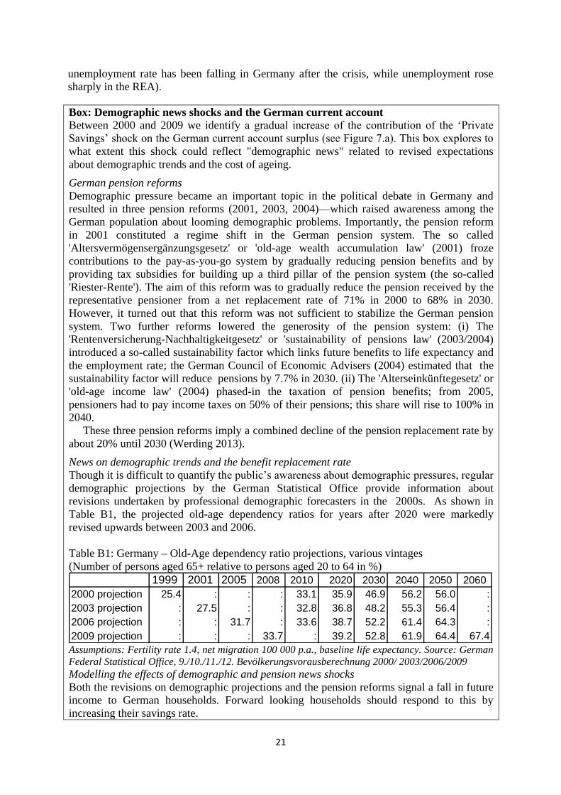
21

unemployment rate has been falling in Germany after the crisis, while unemployment rose

sharply in the REA).

Box: Demographic news shocks and the German current account

Between 2000 and 2009 we identify a gradual increase of the contribution of the ‘Private

Savings’ shock on the German current account surplus (see Figure 7.a). This box explores to

what extent this shock could reflect "demographic news" related to revised expectations

about demographic trends and the cost of ageing.

German pension reforms

Demographic pressure became an important topic in the political debate in Germany and

resulted in three pension reforms (2001, 2003, 2004)—which raised awareness among the

German population about looming demographic problems. Importantly, the pension reform

in 2001 constituted a regime shift in the German pension system. The so called

'Altersvermögensergänzungsgesetz' or 'old-age wealth accumulation law' (2001) froze

contributions to the pay-as-you-go system by gradually reducing pension benefits and by

providing tax subsidies for building up a third pillar of the pension system (the so-called

'Riester-Rente'). The aim of this reform was to gradually reduce the pension received by the

representative pensioner from a net replacement rate of 71% in 2000 to 68% in 2030.

However, it turned out that this reform was not sufficient to stabilize the German pension

system. Two further reforms lowered the generosity of the pension system: (i) The

'Rentenversicherung-Nachhaltigkeitgesetz' or 'sustainability of pensions law' (2003/2004)

introduced a so-called sustainability factor which links future benefits to life expectancy and

the employment rate; the German Council of Economic Advisers (2004) estimated that the

sustainability factor will reduce pensions by 7.7% in 2030. (ii) The 'Alterseinkünftegesetz' or

'old-age income law' (2004) phased-in the taxation of pension benefits; from 2005,

pensioners had to pay income taxes on 50% of their pensions; this share will rise to 100% in

2040.

These three pension reforms imply a combined decline of the pension replacement rate by

about 20% until 2030 (Werding 2013).

News on demographic trends and the benefit replacement rate

Though it is difficult to quantify the public’s awareness about demographic pressures, regular

demographic projections by the German Statistical Office provide information about

revisions undertaken by professional demographic forecasters in the 2000s. As shown in

Table B1, the projected old-age dependency ratios for years after 2020 were markedly

revised upwards between 2003 and 2006.

Table B1: Germany – Old-Age dependency ratio projections, various vintages

(Number of persons aged 65+ relative to persons aged 20 to 64 in %)

1999 2001 2005 2008 2010 2020 2030 2040 2050 2060

2000 projection 25.4 : : : 33.1 35.9 46.9 56.2 56.0 :

2003 projection : 27.5 : : 32.8 36.8 48.2 55.3 56.4 :

2006 projection : : 31.7 : 33.6 38.7 52.2 61.4 64.3 :

2009 projection : : : 33.7 : 39.2 52.8 61.9 64.4 67.4 Assumptions: Fertility rate 1.4, net migration 100 000 p.a., baseline life expectancy. Source: German

Federal Statistical Office, 9./10./11./12. Bevölkerungsvorausberechnung 2000/ 2003/2006/2009

Modelling the effects of demographic and pension news shocks

Both the revisions on demographic projections and the pension reforms signal a fall in future

income to German households. Forward looking households should respond to this by

increasing their savings rate.

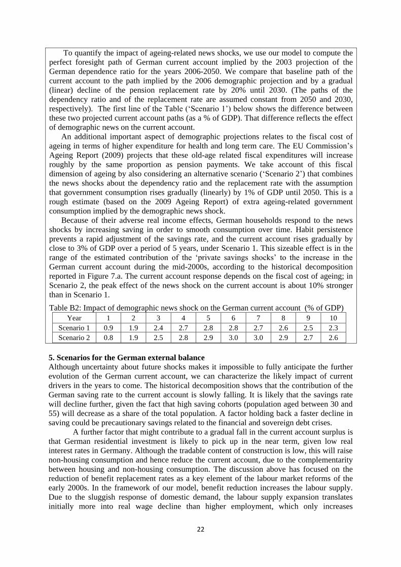
22

To quantify the impact of ageing-related news shocks, we use our model to compute the

perfect foresight path of German current account implied by the 2003 projection of the

German dependence ratio for the years 2006-2050. We compare that baseline path of the

current account to the path implied by the 2006 demographic projection and by a gradual

(linear) decline of the pension replacement rate by 20% until 2030. (The paths of the

dependency ratio and of the replacement rate are assumed constant from 2050 and 2030,

respectively). The first line of the Table (‘Scenario 1’) below shows the difference between

these two projected current account paths (as a % of GDP). That difference reflects the effect

of demographic news on the current account.

An additional important aspect of demographic projections relates to the fiscal cost of

ageing in terms of higher expenditure for health and long term care. The EU Commission’s

Ageing Report (2009) projects that these old-age related fiscal expenditures will increase

roughly by the same proportion as pension payments. We take account of this fiscal

dimension of ageing by also considering an alternative scenario (‘Scenario 2’) that combines

the news shocks about the dependency ratio and the replacement rate with the assumption

that government consumption rises gradually (linearly) by 1% of GDP until 2050. This is a

rough estimate (based on the 2009 Ageing Report) of extra ageing-related government

consumption implied by the demographic news shock.

Because of their adverse real income effects, German households respond to the news

shocks by increasing saving in order to smooth consumption over time. Habit persistence

prevents a rapid adjustment of the savings rate, and the current account rises gradually by

close to 3% of GDP over a period of 5 years, under Scenario 1. This sizeable effect is in the

range of the estimated contribution of the ‘private savings shocks’ to the increase in the

German current account during the mid-2000s, according to the historical decomposition

reported in Figure 7.a. The current account response depends on the fiscal cost of ageing; in

Scenario 2, the peak effect of the news shock on the current account is about 10% stronger

than in Scenario 1.

Table B2: Impact of demographic news shock on the German current account (% of GDP)

Year 1 2 3 4 5 6 7 8 9 10

Scenario 1 0.9 1.9 2.4 2.7 2.8 2.8 2.7 2.6 2.5 2.3

Scenario 2 0.8 1.9 2.5 2.8 2.9 3.0 3.0 2.9 2.7 2.6

5. Scenarios for the German external balance

Although uncertainty about future shocks makes it impossible to fully anticipate the further

evolution of the German current account, we can characterize the likely impact of current

drivers in the years to come. The historical decomposition shows that the contribution of the

German saving rate to the current account is slowly falling. It is likely that the savings rate

will decline further, given the fact that high saving cohorts (population aged between 30 and

55) will decrease as a share of the total population. A factor holding back a faster decline in

saving could be precautionary savings related to the financial and sovereign debt crises.

A further factor that might contribute to a gradual fall in the current account surplus is

that German residential investment is likely to pick up in the near term, given low real

interest rates in Germany. Although the tradable content of construction is low, this will raise

non-housing consumption and hence reduce the current account, due to the complementarity

between housing and non-housing consumption. The discussion above has focused on the

reduction of benefit replacement rates as a key element of the labour market reforms of the

early 2000s. In the framework of our model, benefit reduction increases the labour supply.

Due to the sluggish response of domestic demand, the labour supply expansion translates

initially more into real wage decline than higher employment, which only increases

23

gradually. The fall in wage and production costs improves the price competitiveness of

German goods in foreign and domestic markets and improves the German current account.

However, the model suggests that the positive effect of permanent labour market reform on

the German current account is only temporary, since employment and associated wage

increases stimulate domestic demand (private consumption). According to the model

estimates, the current account increase reaches its maximum around 7 years after the reform.

After that, the current account declines gradually in response to growing domestic demand.

This implies that the contribution of past labour market reforms to the current account surplus

is likely to fall in future years. In addition the policy debates in Germany about the

distributional impact of the labour market reforms has led to plans by the new German

government to introduce a minimum wage law which is likely to further increase German

wages. Moreover, structural reforms currently undertaken in REA countries will boost REA

growth and competitiveness, and accelerate the erosion of Germany's competitive advantage.

The contribution of fiscal policy shocks for the German current account has been modest

during the estimation period. However, in view of the current discussions in Germany about

the need to raise public infrastructure investment, future fiscal policy too may contribute to a

reduction in the German external surplus.

The German non-tradables (services) sector lacks competition (barriers to entry into

the retail, crafts and health sectors), and it is sometimes argued that reforms boosting

competition and productivity in the German non-tradables sector (services) would lower the

German external surplus. The model here cannot be used to evaluate that view, as it does not

include a non-tradables sector. However, several recent papers have studied the effects of

structural reforms in the non-tradables sector (modeled as a positive shock to non-tradables

productivity or a reduction in the mark ups changed by firms that produce non-tradables);

see, e.g., Forni et al. (2010), Vogel (2011, 2013) and Gomes et al. (2013) who use rich DSGE

models of open economies that closely resemble the model used here. These analyses

suggest that reform in the non-tradables sector has a strong positive effect on GDP, but that

the effect on net exports is modest—in fact, net exports may actually rise. The reason for this

is that the domestic tradable good producing sector uses non-tradable inputs—hence,

measures that boost the efficiency of the non-tradables sector improve a country’s external

competitiveness.17

6. Conclusions

We have developed a three-country DSGE model and estimated that model using quarterly

1995-2013 data for Germany, the rest of the Euro Area (REA) and the rest of the world

(ROW). We used that model to analyze the causes of Germany’s substantial and persistent

current account surplus, and its effect on the REA. Our results show that simple mono-causal

explanations of the German surplus are insufficient. The surplus reflects a succession of

distinct shocks. According to our estimates, the most important factors driving the German

surplus were positive shocks to the German saving rate and to ROW demand for German

exports, as well as German labour market reforms and other positive German aggregate

supply shocks. Those shocks had a noticeable negative effect on REA net exports, but only a

modest effect on REA real activity. We expect the contribution of past German labour market

reforms to the current account surplus to decline in future years as wage growth picks up

again. One policy conclusion from our analysis could be that similar reforms are needed in

EA deficit countries. Structural reforms in the REA would boost growth and improve external

17 Dustmann et al. (2014) document that low wage growth in the German non-tradables sector contributed to the

competitiveness of the German exports sector--more than 70% of the total input used by the German exports

sector are domestically produced. These strong domestic input linkages suggest that an aggregative model

(without non-tradables vs. tradables distinction) may be suited for understanding the German macroeconomy.

24

balances there, eroding Germany's competitive advantage. Illustrative model simulations

presented in this paper suggest that increased awareness about future demographic

developments and pension generosity contributed to the German current account surplus. To

the extent that this holds, it would not call for corrective policy actions. Regarding public

demand, Germany's sound fiscal position provides space for a less restrictive fiscal policy;

the rise in German demand would reduce the external surplus and help to achieve a

rebalancing in the EA, albeit by a modest amount.

25

REFERENCES

Adalet, M., B. Eichengreen (2007): "Current account reversals--always a problem?", In: R.

Clarida (ed.), ‘G7 Current Account Imbalances: Sustainability and Adjustment’, Chicago:

University of Chicago Press, pp.205-242.

Adolfson, M., S. Laséen, J.Lindé, M. Villani (2007): "Bayesian estimation of an open economy

DSGE model with incomplete pass-through", Journal of International Economics. Journal of

International Economics 72, 481-511.

Adjemian, S., H. Bastani, M. Juillard, F. Karamé, J. Maih, F. Mihoubi, G. Perendia, M. Ratto, S.

Villemot (2011): "DYNARE: Reference Manual, Version 4". DYNARE Working Paper

Series, 1.

Aizenman, J. and Y. Jinjarak (2013): "Real estate valuation, current account and credit growth

patterns, before and after the 2008-09 crisis", NBER Working Paper No 19190.

Backus, D., P. Kehoe, F. Kydland (1992): "International real business cycles", Journal of

Political Economy 100, 745-775.

Beetsma, R. and M. Giuliodori (2011): "The effects of government purchases shocks: review and

estimates for the EU", Economic Journal 121, F4-F32.

Buera, F., B. Moll (2012): "Aggregate Implications of a Credit Crunch", NBER WP 17775.

Bussière, M., M. Fratzscher, G. Müller (2010): "Productivity shocks, budget deficits and the

current account", Journal of International Money and Finance 29, 1562-1579.

Carton, B., K. Hervé (2012): "Euro area real effective exchange rate misalignements", La Lettre

du CEPII, No 319 - 19 April 2012

Chen, R., G-.M. Milesi-Ferretti, T. Tressel (2012): "External imbalances in the euro area," IMF

Working Paper 12/236.

Chinn, M., B. Eichengreen and H. Ito (2013): "A forensic analysis of global imbalances",

Working Paper, University of Wisconsin.

Christiano, L., M. Eichenbaum, C. Evans (2005): "Nominal rigidities and the dynamic effects of

a shock to monetary policy", Journal of Political Economy 113, 1–45.

Corsetti, G., G. Müller (2006): "Budget deficits and current accounts", Economic Policy 26,

598-638.

Deutsche Bundesbank (2011): "Germany's external position against the background of increasing

economic policy surveillance", Monthly Report, October 2011, pp. 41-59.

Deutsches Institut für Wirtschaftsforschung (2013): "Investitionen für mehr Wachstum-- Eine

Zukunftsagenda für Deutschland", DIW Wochenbericht 26.

Dustmann, C., B. Fitzenberger, U. Schönberg, A. Spitz-Oeber (2014): "From sick man of Europe

to Economic superstar: Germany’s resurgent economy", Journal of Economic Perspectives

28, 167-188.

Erceg, C., L. Guerrieri, C. Gust (2006): "SIGMA: a new open economy model for policy

analysis", International Journal of Central Banking 2, 1-50.

European Commission (2009): "Ageing report: economic and budgetary projections for the EU-

27 member states 2008-2060".

European Commission (2012a): "Current account surpluses in the EU", European Economy

9/2012.

European Commission (2012b): "Scoreboard for the surveillance of macroeconomic

imbalances". European Economy Occasional Paper 92.

European Commission (2013): "Alert Mechanism Report 2014."

European Commission (2014): "Macroeconomic imbalances - Germany 2014", European

Economy Occasional Paper no.174.

Fernández-Villaverde, J., L. Garicano, T. Santos (2013): "Political credit cycles: the case of the

Eurozone", Journal of Economic Perspectives 27, 145-166.

Fisher, J. (2006): "The dynamic effects of neutral and investment-specific technology shocks",

Journal of Political Economy 114, 413-52.

Fornaro, L. (2013): "Debt deleveraging, debt Relief and liquidity traps," Manuscript, CREI.

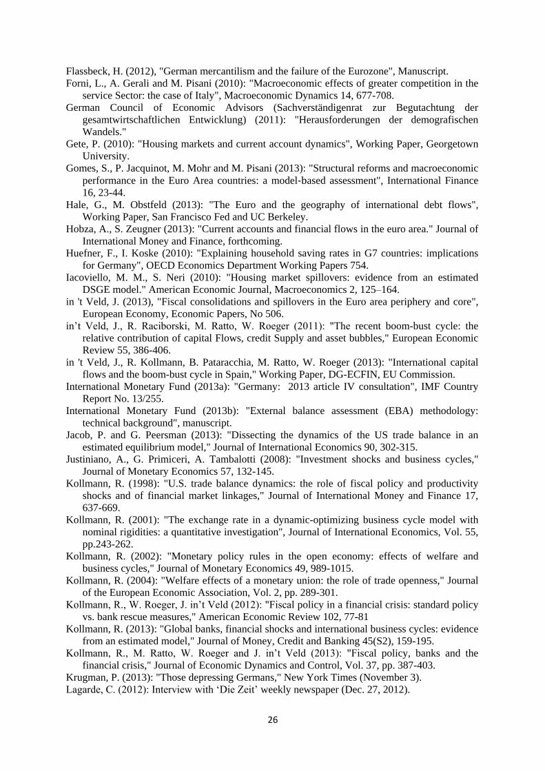
26

Flassbeck, H. (2012), "German mercantilism and the failure of the Eurozone", Manuscript.

Forni, L., A. Gerali and M. Pisani (2010): "Macroeconomic effects of greater competition in the

service Sector: the case of Italy", Macroeconomic Dynamics 14, 677-708.

German Council of Economic Advisors (Sachverständigenrat zur Begutachtung der

gesamtwirtschaftlichen Entwicklung) (2011): "Herausforderungen der demografischen

Wandels."

Gete, P. (2010): "Housing markets and current account dynamics", Working Paper, Georgetown

University.

Gomes, S., P. Jacquinot, M. Mohr and M. Pisani (2013): "Structural reforms and macroeconomic

performance in the Euro Area countries: a model‐based assessment", International Finance

16, 23-44.

Hale, G., M. Obstfeld (2013): "The Euro and the geography of international debt flows",

Working Paper, San Francisco Fed and UC Berkeley.

Hobza, A., S. Zeugner (2013): "Current accounts and financial flows in the euro area." Journal of

International Money and Finance, forthcoming.

Huefner, F., I. Koske (2010): "Explaining household saving rates in G7 countries: implications

for Germany", OECD Economics Department Working Papers 754.

Iacoviello, M. M., S. Neri (2010): "Housing market spillovers: evidence from an estimated

DSGE model." American Economic Journal, Macroeconomics 2, 125–164.

in 't Veld, J. (2013), "Fiscal consolidations and spillovers in the Euro area periphery and core",

European Economy, Economic Papers, No 506.

in’t Veld, J., R. Raciborski, M. Ratto, W. Roeger (2011): "The recent boom-bust cycle: the

relative contribution of capital Flows, credit Supply and asset bubbles," European Economic

Review 55, 386-406.

in 't Veld, J., R. Kollmann, B. Pataracchia, M. Ratto, W. Roeger (2013): "International capital

flows and the boom-bust cycle in Spain," Working Paper, DG-ECFIN, EU Commission.

International Monetary Fund (2013a): "Germany: 2013 article IV consultation", IMF Country

Report No. 13/255.

International Monetary Fund (2013b): "External balance assessment (EBA) methodology:

technical background", manuscript.

Jacob, P. and G. Peersman (2013): "Dissecting the dynamics of the US trade balance in an

estimated equilibrium model," Journal of International Economics 90, 302-315.

Justiniano, A., G. Primiceri, A. Tambalotti (2008): "Investment shocks and business cycles,"

Journal of Monetary Economics 57, 132-145.

Kollmann, R. (1998): "U.S. trade balance dynamics: the role of fiscal policy and productivity

shocks and of financial market linkages," Journal of International Money and Finance 17,

637-669.

Kollmann, R. (2001): "The exchange rate in a dynamic-optimizing business cycle model with

nominal rigidities: a quantitative investigation", Journal of International Economics, Vol. 55,

pp.243-262.

Kollmann, R. (2002): "Monetary policy rules in the open economy: effects of welfare and

business cycles," Journal of Monetary Economics 49, 989-1015.

Kollmann, R. (2004): "Welfare effects of a monetary union: the role of trade openness," Journal

of the European Economic Association, Vol. 2, pp. 289-301.

Kollmann, R., W. Roeger, J. in’t Veld (2012): "Fiscal policy in a financial crisis: standard policy

vs. bank rescue measures," American Economic Review 102, 77-81

Kollmann, R. (2013): "Global banks, financial shocks and international business cycles: evidence

from an estimated model," Journal of Money, Credit and Banking 45(S2), 159-195.

Kollmann, R., M. Ratto, W. Roeger and J. in’t Veld (2013): "Fiscal policy, banks and the

financial crisis," Journal of Economic Dynamics and Control, Vol. 37, pp. 387-403.

Krugman, P. (2013): "Those depressing Germans," New York Times (November 3).

Lagarde, C. (2012): Interview with ‘Die Zeit’ weekly newspaper (Dec. 27, 2012).

27

Lane, P. (2012): "Capital flows in the Euro Area," Working Paper, Trinity College Dublin.

Louanges, M. (2005): "Is Germany on its way to regaining its European benchmark status,"

PIMCO European Perspectives (September 2005).

McCallum, B. (1994): "A reconsideration of the uncovered interest parity relationship," Journal

of Monetary Economics 33, 105-132.

Mendoza, E. (2010): "Sudden stops, financial crises, and leverage," American Economic Review

100, 1941–1966.

Milesi-Ferretti, GM, A. Razin (1998): "Sharp reductions in current account deficits--An

empirical analysis," European Economic Review 42, 897-908.

Obstfeld, M., K. Rogoff (1996): "Foundations of international macroeconomics", MIT Press.

Obstfeld, M. and K. Rogoff (2010): "Global imbalances and the financial crisis: products of

common causes." In: Glick, R., Spiegel, M. (Eds.), Asia and the Global Financial Crisis.

Federal Reserve Bank of San Francisco, San Francisco, pp.131-172.

Obstfeld, M. (2012): "Does the current account still matter?” American Economic Review 102,

1-23.

Organisation for Economic Co-operation and Development (2013): "Employment and labor

market statistics."

Pytlarczyk, E. (2005): "An estimated DSGE model for the German economy within the euro

area," Bundesbank Discussion Paper No 33/2005.

Ratto M, W. Roeger and J. in ’t Veld (2009) , “QUEST III: an estimated open-economy DSGE

model of the Euro Area with fiscal and monetary policy”, Economic Modelling 26, 222-233

Reis, R. (2013): "The Portuguese slump-crash and the Euro-crisis," Brookings Papers on

Economic Activity, 143-193.

Sinn, H-W. (2003): "The laggard of Europe," CESifo Forum Vol. 4, Special Issue No. 1.

Sinn, H.-W. (2006): "The pathological export boom and the bazaar effect: how to solve the

German puzzle," The World Economy, Vol. 29, No. 9, pp. 1157-1175.

Sinn, H.-W. (2010): "Rescuing Europe," CESifo Forum, Vol. 11, special issue, pp.1-22.

Sinn, H.-W. (2013): "Jetzt hilft nur durchwursteln," ifo Standpunkt 150.

Statistisches Bundesamt (2003): "9. Bevölkerungsvorausberechnung."

Statistisches Bundesamt (2006): "10. Bevölkerungsvorausberechnung."

Statistisches Bundesamt (2009): "11. Bevölkerungsvorausberechnung."

Statistisches Bundesamt (2012): "12. Bevölkerungsvorausberechnung."

U.S. Department of the Treasury (2013): "Report to congress on international economic and

exchange rate policies." (October 30, 2013)

Vogel, L. (2011): "Structural reforms and external rebalancing in the Euro Area: A model-based

analysis," European Economy, Economic Papers 433.

Vogel, L. (2013): "Nontradable sector reform and external rebalancing in Monetary Union: a

model-based analysis," Working Paper, DG-ECFIN, European Commission.

Werding, M. (2013): "Alterssicherung, Arbeitsmarktdynamik und neue Reformen: Wie das

Rentensystem stabilisiert werden kann," Bertelsmann Stiftung: Gütersloh

Wolf, M. (2013): "Germany is a weight on the world," Financial Times (November 5).

Zettelmeyer, J. (1997): "EMU and long interest rates in Germany," In: P. Welfens (ed),

‘European Monetary Union Transition, International Impact and Policy Options’, New York:

Springer Verlag, pp. 13-58.

28

Figure 1: The German current account, net exports, consumption and investment (1.a) Current Account, net exports, net transfers

and incomes from rest of world, % of GDP (1.b) International Investment Position, % of GDP

-4

-2

0

2

4

6

8

10 External accounts (% of GDP)

Trade balance Current account0

5

10

15

20

25

30

35

40

45 IIP (% of GDP)

(1.c) National saving, investment and CA, % of GDP (1.d) Private & Government S & I, in % of GDP

(1.e) Net export, Y-C-G, I, % of GDP (1.f) Private & Government consumption, % of GDP

(1.h) Total net exports of Germany; German NX to REA;

(1.g) Exports and Imports, % of GDP REA net imports; EA net exports

29

Figure 2: Real activity (DE: Germany) (2.a) Germany: real GDP & aggregate demand components (2.b) YoY GDP growth rates (Germany, REA, ROW)

80

85

90

95

100

105

110

115

120

125

130

95 97 99 01 03 05 07 09 11 13

1995=100

Year

Y

C

G

I

Figure 3: Interest rates, inflation, exchange rates (DE: Germany) (3.a) Nominal interest rates: DE, REA, ROW, %p.a. (3.b) YoY growth of GDP deflator, %

(3.c) Nominal effective exchange rate: DE vs. REA (3.d) Real exchange rates: DE-REA; DE-ROW

Rise: DE appreciat.; exch. rate 1999-2012 normalized at 1 Rise: DE appreciation

30

Figure 4: Wages, unit labor costs, unemployment benefits (DE: Germany) (4.a) Nominal compensation per employee, % p.a. growth (4.b) Real compensation per employee, % p.a. growth

(4.c) Nominal unit labor cost, DE & EA (2005=100) (4.d) Average unemployment benefit ratio, Germany

Figure 5: Demographics and pensions: Germany (5.a) Germany, dependency ration, in % (5.b) Germany, average pension replacement rate, in %

2011-2060: projections (German Council of Economic

Advisors (2011))

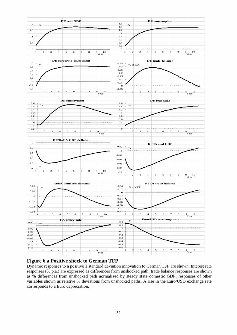
31

0

0.5

1

1.5

2

1 2 3 4 5 6 7 8 9 10

%

Year

DE real GDP

0

0.2

0.4

0.6

0.8

1

1.2

1.4

1.6

1 2 3 4 5 6 7 8 9 10

%

Year

DE consumption

-0.4

-0.2

0

0.2

0.4

0.6

0.8

1

1 2 3 4 5 6 7 8 9 10

%

Year

DE corporate investment

-0.05

0

0.05

0.1

0.15

0.2

0.25

0.3

0.35

1 2 3 4 5 6 7 8 9 10

% of GDP

Year

DE trade balance

-0.2

-0.1

0

0.1

0.2

0.3

0.4

0.5

0.6

1 2 3 4 5 6 7 8 9 10

%

Year

DE employment

0

0.2

0.4

0.6

0.8

1

1.2

1.4

1.6

1 2 3 4 5 6 7 8 9 10

%

Year

DE real wage

-1

-0.8

-0.6

-0.4

-0.2

0

1 2 3 4 5 6 7 8 9 10

%

Year

DE/RoEA GDP deflator

-0.14

-0.12

-0.1

-0.08

-0.06

-0.04

-0.02

0

0.02

1 2 3 4 5 6 7 8 9 10

pp

Year

EA policy rate

-0.6

-0.5

-0.4

-0.3

-0.2

-0.1

0

0.1

0.2

1 2 3 4 5 6 7 8 9 10

%

Year

Euro/USD exchange rate

-0.1

-0.08

-0.06

-0.04

-0.02

0

0.02

1 2 3 4 5 6 7 8 9 10

%

Year

RoEA real GDP

-0.03

-0.02

-0.01

0

0.01

0.02

1 2 3 4 5 6 7 8 9 10

%

Year

RoEA domestic demand

-0.12

-0.1

-0.08

-0.06

-0.04

-0.02

0

0.02

0.04

1 2 3 4 5 6 7 8 9 10

% of GDP

Year

RoEA trade balance

Figure 6.a Positive shock to German TFP Dynamic responses to a positive 1 standard deviation innovation to German TFP are shown. Interest rate

responses (% p.a.) are expressed as differences from unshocked path; trade balance responses are shown

as % differences from unshocked path normalized by steady state domestic GDP; responses of other

variables shown as relative % deviations from unshocked paths. A rise in the Euro/USD exchange rate

corresponds to a Euro depreciation.

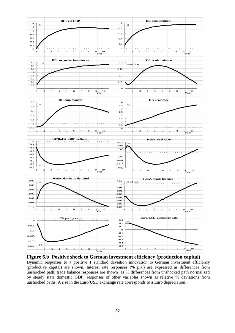
32

0

0.2

0.4

0.6

0.8

1

1.2

1.4

1 2 3 4 5 6 7 8 9 10

%

Year

DE real GDP

0

0.2

0.4

0.6

0.8

1

1 2 3 4 5 6 7 8 9 10

%

Year

DE consumption

0

0.2

0.4

0.6

0.8

1

1.2

1.4

1.6

1 2 3 4 5 6 7 8 9 10

%

Year

DE corporate investment

0

0.05

0.1

0.15

0.2

1 2 3 4 5 6 7 8 9 10

% of GDP

Year

DE trade balance

-0.1

0

0.1

0.2

0.3

0.4

0.5

1 2 3 4 5 6 7 8 9 10

%

Year

DE employment

0

0.5

1

1.5

2

2.5

3

3.5

4

1 2 3 4 5 6 7 8 9 10

%

Year

DE real wage

-0.8

-0.7

-0.6

-0.5

-0.4

-0.3

-0.2

-0.1

0

1 2 3 4 5 6 7 8 9 10

%

Year

DE/RoEA GDP deflator

-0.025

-0.02

-0.015

-0.01

-0.005

0

1 2 3 4 5 6 7 8 9 10

pp

Year

EA policy rate

-0.5

-0.4

-0.3

-0.2

-0.1

0

0.1

0.2

0.3

1 2 3 4 5 6 7 8 9 10

%

Year

Euro/USD exchange rate

-0.02

-0.015

-0.01

-0.005

0

0.005

0.01

0.015

1 2 3 4 5 6 7 8 9 10

%

Year

RoEA real GDP

0

0.01

0.02

0.03

0.04

0.05

0.06

1 2 3 4 5 6 7 8 9 10

%

Year

RoEA domestic demand

-0.07

-0.06

-0.05

-0.04

-0.03

-0.02

-0.01

0

0.01

1 2 3 4 5 6 7 8 9 10

% of GDP

Year

RoEA trade balance

Figure 6.b Positive shock to German investment efficiency (production capital) Dynamic responses to a positive 1 standard deviation innovation to German investment efficiency

(productive capital) are shown. Interest rate responses (% p.a.) are expressed as differences from

unshocked path; trade balance responses are shown as % differences from unshocked path normalized

by steady state domestic GDP; responses of other variables shown as relative % deviations from

unshocked paths. A rise in the Euro/USD exchange rate corresponds to a Euro depreciation.

33

0

0.2

0.4

0.6

0.8

1

1.2

1 2 3 4 5 6 7 8 9 10

%

Year

DE real GDP

-0.1

-0.05

0

0.05

0.1

0.15

0.2

0.25

1 2 3 4 5 6 7 8 9 10

%

Year

DE consumption

-0.4

-0.2

0

0.2

0.4

0.6

0.8

1 2 3 4 5 6 7 8 9 10

%

Year

DE corporate investment

0

0.05

0.1

0.15

0.2

0.25

0.3

0.35

0.4

1 2 3 4 5 6 7 8 9 10

% of GDP

Year

DE trade balance

0

0.2

0.4

0.6

0.8

1

1.2

1.4

1 2 3 4 5 6 7 8 9 10

%

Year

DE employment

-0.6

-0.5

-0.4

-0.3

-0.2

-0.1

0

1 2 3 4 5 6 7 8 9 10

%

Year

DE real wage

-0.6

-0.5

-0.4

-0.3

-0.2

-0.1

0

1 2 3 4 5 6 7 8 9 10

%

Year

DE/RoEA GDP deflator

-0.025

-0.02

-0.015

-0.01

-0.005

0

1 2 3 4 5 6 7 8 9 10

pp

Year

EA policy rate

-0.6

-0.5

-0.4

-0.3

-0.2

-0.1

0

0.1

0.2

0.3

1 2 3 4 5 6 7 8 9 10

%

Year

Euro/USD exchange rate

-0.025

-0.02

-0.015

-0.01

-0.005

0

0.005

0.01

0.015

1 2 3 4 5 6 7 8 9 10

%

Year

RoEA real GDP

0

0.01

0.02

0.03

0.04

0.05

1 2 3 4 5 6 7 8 9 10

%

Year

RoEA domestic demand

-0.1

-0.08

-0.06

-0.04

-0.02

0

1 2 3 4 5 6 7 8 9 10

% of GDP

Year

RoEA trade balance

Figure 6.c Cut in German unemployment benefit ratio Dynamic responses to a permanent 1 percentage point reduction in the German unemployment benefit

ratio are shown. Interest rate responses (% p.a.) are expressed as differences from unshocked path; trade

balance responses are shown as % differences from unshocked path normalized by steady state domestic

GDP; responses of other variables shown as relative % deviations from unshocked paths. A rise in the

Euro/USD exchange rate corresponds to a Euro depreciation.

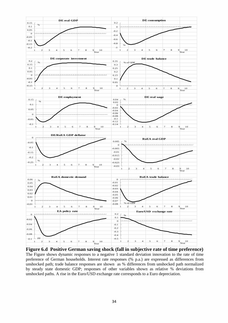
34

-0.2

-0.15

-0.1

-0.05

0

0.05

0.1

0.15

1 2 3 4 5 6 7 8 9 10

%

Year

DE real GDP

-1

-0.8

-0.6

-0.4

-0.2

0

0.2

1 2 3 4 5 6 7 8 9 10

%

Year

DE consumption

-0.15

-0.1

-0.05

0

0.05

0.1

0.15

0.2

1 2 3 4 5 6 7 8 9 10

%

Year

DE corporate investment

0

0.05

0.1

0.15

0.2

0.25

0.3

0.35

1 2 3 4 5 6 7 8 9 10

% of GDP

Year

DE trade balance

-0.1

-0.05

0

0.05

0.1

0.15

1 2 3 4 5 6 7 8 9 10

%

Year

DE employment

-0.14

-0.12

-0.1

-0.08

-0.06

-0.04

-0.02

0

0.02

0.04

1 2 3 4 5 6 7 8 9 10

%

Year

DE real wage

-0.25

-0.2

-0.15

-0.1

-0.05

0

1 2 3 4 5 6 7 8 9 10

%

Year

DE/RoEA GDP deflator

-0.1

-0.08

-0.06

-0.04

-0.02

0

1 2 3 4 5 6 7 8 9 10

pp

Year

EA policy rate

-0.5

-0.4

-0.3

-0.2

-0.1

0

0.1

0.2

1 2 3 4 5 6 7 8 9 10

%

Year

Euro/USD exchange rate

-0.03

-0.025

-0.02

-0.015

-0.01

-0.005

0

0.005

1 2 3 4 5 6 7 8 9 10

%

Year

RoEA real GDP

-0.01

0

0.01

0.02

0.03

0.04

0.05

0.06

1 2 3 4 5 6 7 8 9 10

%

Year

RoEA domestic demand

-0.08

-0.07

-0.06

-0.05

-0.04

-0.03

-0.02

-0.01

0

1 2 3 4 5 6 7 8 9 10

% of GDP

Year

RoEA trade balance

Figure 6.d Positive German saving shock (fall in subjective rate of time preference) The Figure shows dynamic responses to a negative 1 standard deviation innovation to the rate of time

preference of German households. Interest rate responses (% p.a.) are expressed as differences from

unshocked path; trade balance responses are shown as % differences from unshocked path normalized

by steady state domestic GDP; responses of other variables shown as relative % deviations from

unshocked paths. A rise in the Euro/USD exchange rate corresponds to a Euro depreciation.

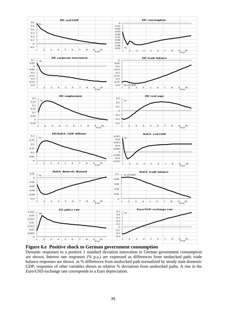
35

-0.1

0

0.1

0.2

0.3

0.4

0.5

0.6

1 2 3 4 5 6 7 8 9 10

%

Year

DE real GDP

-0.09

-0.08

-0.07

-0.06

-0.05

-0.04

-0.03

-0.02

-0.01

0

1 2 3 4 5 6 7 8 9 10

%

Year

DE consumption

-0.3

-0.25

-0.2

-0.15

-0.1

-0.05

0

0.05

0.1

1 2 3 4 5 6 7 8 9 10

%

Year

DE corporate investment

-0.4

-0.35

-0.3

-0.25

-0.2

-0.15

-0.1

-0.05

0

1 2 3 4 5 6 7 8 9 10

% of GDP

Year

DE trade balance

-0.05

0

0.05

0.1

0.15

0.2

0.25

0.3

1 2 3 4 5 6 7 8 9 10

%

Year

DE employment

-0.3

-0.2

-0.1

0

0.1

0.2

0.3

1 2 3 4 5 6 7 8 9 10

%

Year

DE real wage

0

0.05

0.1

0.15

0.2

0.25

0.3

1 2 3 4 5 6 7 8 9 10

%

Year

DE/RoEA GDP deflator

0

0.005

0.01

0.015

0.02

0.025

0.03

0.035

1 2 3 4 5 6 7 8 9 10

pp

Year

EA policy rate

-0.3

-0.2

-0.1

0

0.1

0.2

0.3

0.4

0.5

1 2 3 4 5 6 7 8 9 10

%

Year

Euro/USD exchange rate

-0.015

-0.01

-0.005

0

0.005

0.01

0.015

0.02

0.025

1 2 3 4 5 6 7 8 9 10

%

Year

RoEA real GDP

-0.1

-0.08

-0.06

-0.04

-0.02

0

0.02

1 2 3 4 5 6 7 8 9 10

%

Year

RoEA domestic demand

0

0.02

0.04

0.06

0.08

0.1

1 2 3 4 5 6 7 8 9 10

% of GDP

Year

RoEA trade balance

Figure 6.e Positive shock to German government consumption

Dynamic responses to a positive 1 standard deviation innovation to German government consumption

are shown. Interest rate responses (% p.a.) are expressed as differences from unshocked path; trade

balance responses are shown as % differences from unshocked path normalized by steady state domestic

GDP; responses of other variables shown as relative % deviations from unshocked paths. A rise in the

Euro/USD exchange rate corresponds to a Euro depreciation.

36

0

0.5

1

1.5

2

2.5

3

3.5

1 2 3 4 5 6 7 8 9 10

%

Year

DE real GDP

0

0.5

1

1.5

2

2.5

1 2 3 4 5 6 7 8 9 10

%

Year

DE consumption

-0.6

-0.4

-0.2

0

0.2

0.4

0.6

0.8

1

1 2 3 4 5 6 7 8 9 10

%

Year

DE corporate investment

-0.3

-0.2

-0.1

0

0.1

0.2

0.3

1 2 3 4 5 6 7 8 9 10

% of GDP

Year

DE trade balance

0

0.1

0.2

0.3

0.4

0.5

0.6

0.7

0.8

0.9

1 2 3 4 5 6 7 8 9 10

%

Year

DE employment

-2

0

2

4

6

8

10

12

1 2 3 4 5 6 7 8 9 10

%

Year

DE real wage

-1.4

-1.2

-1

-0.8

-0.6

-0.4

-0.2

0

0.2

0.4

1 2 3 4 5 6 7 8 9 10

%

Year

DE/RoEA GDP deflator

0

0.01

0.02

0.03

0.04

0.05

1 2 3 4 5 6 7 8 9 10

pp

Year

EA policy rate

-0.2

-0.1

0

0.1

0.2

0.3

0.4

1 2 3 4 5 6 7 8 9 10

%

Year

Euro/USD exchange rate

-0.02

-0.01

0

0.01

0.02

0.03

0.04

1 2 3 4 5 6 7 8 9 10

%

Year

RoEA real GDP

-0.1

-0.05

0

0.05

0.1

0.15

1 2 3 4 5 6 7 8 9 10

%

Year

RoEA domestic demand

-0.1

-0.08

-0.06

-0.04

-0.02

0

0.02

0.04

0.06

1 2 3 4 5 6 7 8 9 10

% of GDP

Year

RoEA trade balance

Figure 6.f Positive shock to German government investment

Dynamic responses to a positive 1 standard deviation innovation to German government investment are

shown. Interest rate responses (% p.a.) are expressed as differences from unshocked path; trade balance

responses are shown as % differences from unshocked path normalized by steady state domestic GDP;

responses of other variables shown as relative % deviations from unshocked paths. A rise in the

Euro/USD exchange rate corresponds to a Euro depreciation.

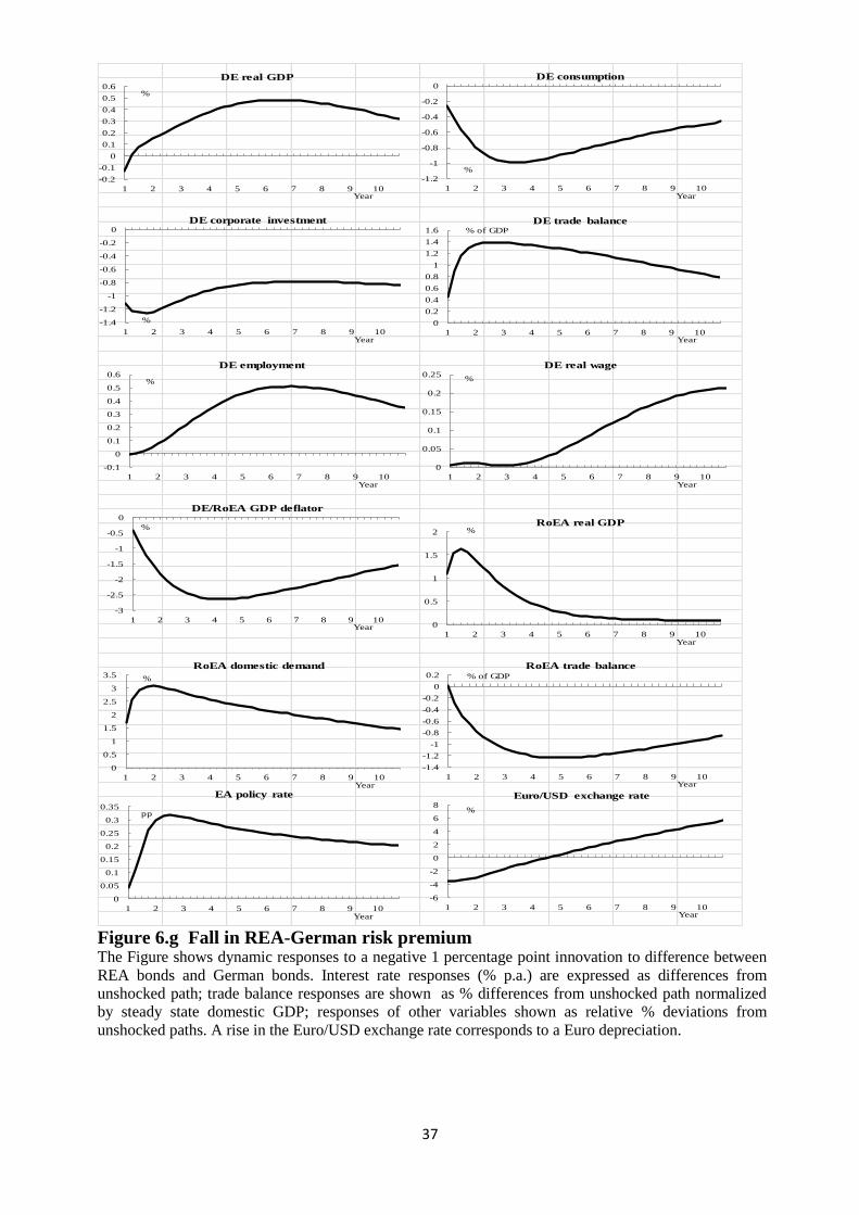
37

-0.2

-0.1

0

0.1

0.2

0.3

0.4

0.5

0.6

1 2 3 4 5 6 7 8 9 10

%

Year

DE real GDP

-1.2

-1

-0.8

-0.6

-0.4

-0.2

0

1 2 3 4 5 6 7 8 9 10

%

Year

DE consumption

-1.4

-1.2

-1

-0.8

-0.6

-0.4

-0.2

0

1 2 3 4 5 6 7 8 9 10

%

Year

DE corporate investment

0

0.2

0.4

0.6

0.8

1

1.2

1.4

1.6

1 2 3 4 5 6 7 8 9 10

% of GDP

Year

DE trade balance

-0.1

0

0.1

0.2

0.3

0.4

0.5

0.6

1 2 3 4 5 6 7 8 9 10

%

Year

DE employment

0

0.05

0.1

0.15

0.2

0.25

1 2 3 4 5 6 7 8 9 10

%

Year

DE real wage

-3

-2.5

-2

-1.5

-1

-0.5

0

1 2 3 4 5 6 7 8 9 10

%

Year

DE/RoEA GDP deflator

0

0.05

0.1

0.15

0.2

0.25

0.3

0.35

1 2 3 4 5 6 7 8 9 10

pp

Year

EA policy rate

-6

-4

-2

0

2

4

6

8

1 2 3 4 5 6 7 8 9 10

%

Year

Euro/USD exchange rate

0

0.5

1

1.5

2

1 2 3 4 5 6 7 8 9 10

%

Year

RoEA real GDP

0

0.5

1

1.5

2

2.5

3

3.5

1 2 3 4 5 6 7 8 9 10

%

Year

RoEA domestic demand

-1.4

-1.2

-1

-0.8

-0.6

-0.4

-0.2

0

0.2

1 2 3 4 5 6 7 8 9 10

% of GDP

Year

RoEA trade balance

Figure 6.g Fall in REA-German risk premium The Figure shows dynamic responses to a negative 1 percentage point innovation to difference between

REA bonds and German bonds. Interest rate responses (% p.a.) are expressed as differences from

unshocked path; trade balance responses are shown as % differences from unshocked path normalized

by steady state domestic GDP; responses of other variables shown as relative % deviations from

unshocked paths. A rise in the Euro/USD exchange rate corresponds to a Euro depreciation.

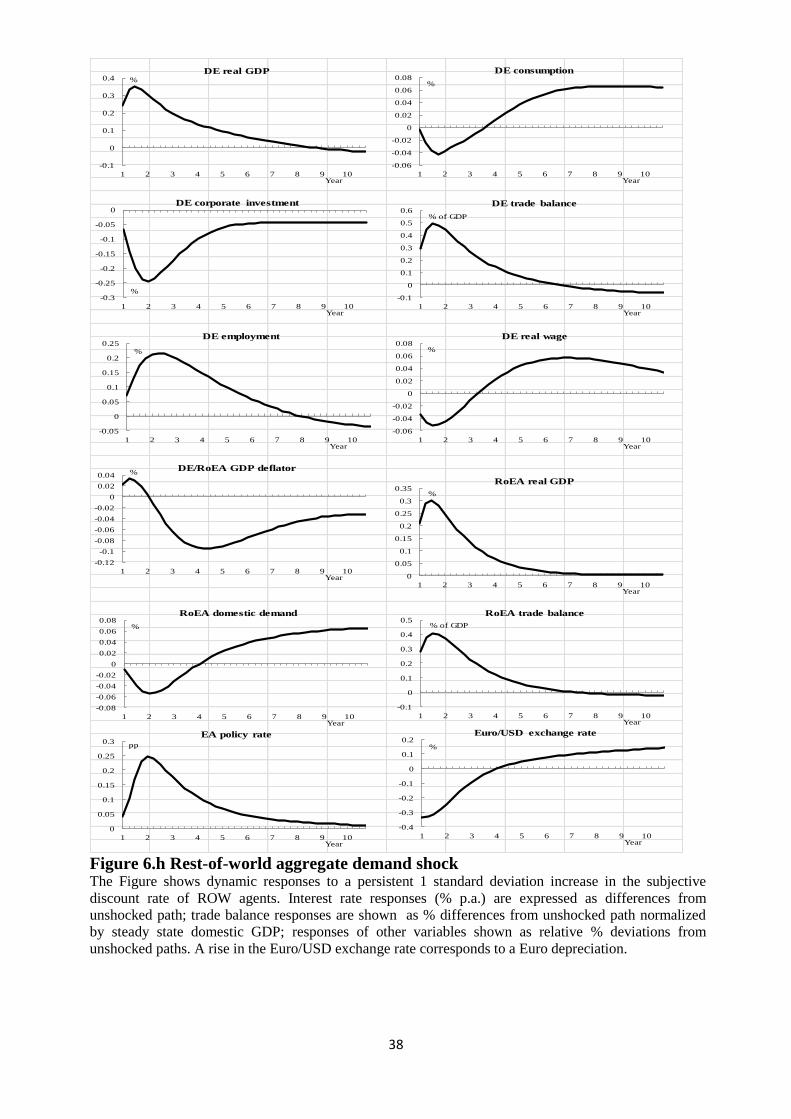
38

-0.1

0

0.1

0.2

0.3

0.4

1 2 3 4 5 6 7 8 9 10

%

Year

DE real GDP

-0.06

-0.04

-0.02

0

0.02

0.04

0.06

0.08

1 2 3 4 5 6 7 8 9 10

%

Year

DE consumption

-0.3

-0.25

-0.2

-0.15

-0.1

-0.05

0

1 2 3 4 5 6 7 8 9 10

%

Year

DE corporate investment

-0.1

0

0.1

0.2

0.3

0.4

0.5

0.6

1 2 3 4 5 6 7 8 9 10

% of GDP

Year

DE trade balance

-0.05

0

0.05

0.1

0.15

0.2

0.25

1 2 3 4 5 6 7 8 9 10

%

Year

DE employment

-0.06

-0.04

-0.02

0

0.02

0.04

0.06

0.08

1 2 3 4 5 6 7 8 9 10

%

Year

DE real wage

-0.12

-0.1

-0.08

-0.06

-0.04

-0.02

0

0.02

0.04

1 2 3 4 5 6 7 8 9 10

%

Year

DE/RoEA GDP deflator

0

0.05

0.1

0.15

0.2

0.25

0.3

1 2 3 4 5 6 7 8 9 10

pp

Year

EA policy rate

-0.4

-0.3

-0.2

-0.1

0

0.1

0.2

1 2 3 4 5 6 7 8 9 10

%

Year

Euro/USD exchange rate

0

0.05

0.1

0.15

0.2

0.25

0.3

0.35

1 2 3 4 5 6 7 8 9 10

%

Year

RoEA real GDP

-0.08

-0.06

-0.04

-0.02

0

0.02

0.04

0.06

0.08

1 2 3 4 5 6 7 8 9 10

%

Year

RoEA domestic demand

-0.1

0

0.1

0.2

0.3

0.4

0.5

1 2 3 4 5 6 7 8 9 10

% of GDP

Year

RoEA trade balance

Figure 6.h Rest-of-world aggregate demand shock The Figure shows dynamic responses to a persistent 1 standard deviation increase in the subjective

discount rate of ROW agents. Interest rate responses (% p.a.) are expressed as differences from

unshocked path; trade balance responses are shown as % differences from unshocked path normalized

by steady state domestic GDP; responses of other variables shown as relative % deviations from

unshocked paths. A rise in the Euro/USD exchange rate corresponds to a Euro depreciation.

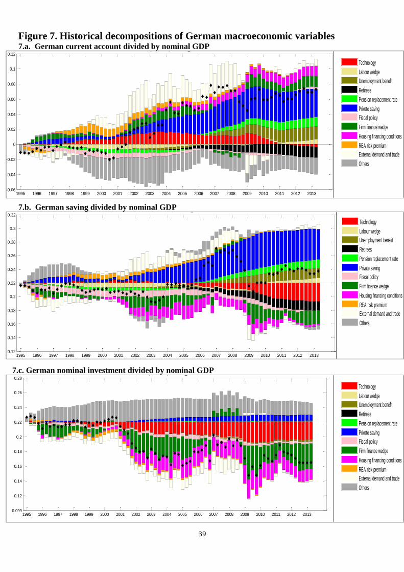
39

Figure 7. Historical decompositions of German macroeconomic variables 7.a. German current account divided by nominal GDP

1995 1996 1997 1998 1999 2000 2001 2002 2003 2004 2005 2006 2007 2008 2009 2010 2011 2012 2013-0.06

-0.04

-0.02

0

0.02

0.04

0.06

0.08

0.1

0.12quarter to quarter DE_CAY

Technology

Labour wedge

Unemployment benefit

Retirees

Pension replacement rate

Private saving

Fiscal policy

Firm finance wedge

Housing financing conditions

REA risk premium

External demand and trade

Others

1995 1996 1997 1998 1999 2000 2001 2002 2003 2004 2005 2006 2007 2008 2009 2010 2011 2012 20130.099

0.12

0.14

0.16

0.18

0.2

0.22

0.24

0.26

0.28quarter to quarter DE_ITOTSN

Technology

Labour wedge

Unemployment benefit

Retirees

Pension replacement rate

Private saving

Fiscal policy

Firm finance wedge

Housing financing conditions

REA risk premium

External demand and trade

Others

7.b. German saving divided by nominal GDP

1995 1996 1997 1998 1999 2000 2001 2002 2003 2004 2005 2006 2007 2008 2009 2010 2011 2012 20130.12

0.14

0.16

0.18

0.2

0.22

0.24

0.26

0.28

0.3

0.32quarter to quarter DE_SY

Technology

Labour wedge

Unemployment benefit

Retirees

Pension replacement rate

Private saving

Fiscal policy

Firm finance wedge

Housing financing conditions

REA risk premium

External demand and trade

Others

1995 1996 1997 1998 1999 2000 2001 2002 2003 2004 2005 2006 2007 2008 2009 2010 2011 2012 20130.099

0.12

0.14

0.16

0.18

0.2

0.22

0.24

0.26

0.28quarter to quarter DE_ITOTSN

Technology

Labour wedge

Unemployment benefit

Retirees

Pension replacement rate

Private saving

Fiscal policy

Firm finance wedge

Housing financing conditions

REA risk premium

External demand and trade

Others

7.c. German nominal investment divided by nominal GDP

1995 1996 1997 1998 1999 2000 2001 2002 2003 2004 2005 2006 2007 2008 2009 2010 2011 2012 20130.099

0.12

0.14

0.16

0.18

0.2

0.22

0.24

0.26

0.28quarter to quarter DE_ITOTSN

Technology

Labour wedge

Unemployment benefit

Retirees

Pension replacement rate

Private saving

Fiscal policy

Firm finance wedge

Housing financing conditions

REA risk premium

External demand and trade

Others

1995 1996 1997 1998 1999 2000 2001 2002 2003 2004 2005 2006 2007 2008 2009 2010 2011 2012 20130.099

0.12

0.14

0.16

0.18

0.2

0.22

0.24

0.26

0.28quarter to quarter DE_ITOTSN

Technology

Labour wedge

Unemployment benefit

Retirees

Pension replacement rate

Private saving

Fiscal policy

Firm finance wedge

Housing financing conditions

REA risk premium

External demand and trade

Others

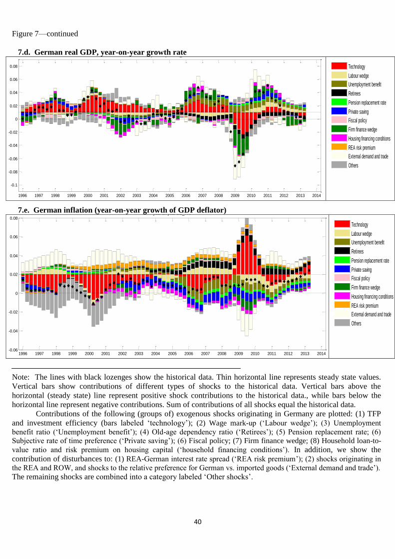
40

Figure 7—continued

7.d. German real GDP, year-on-year growth rate

1996 1997 1998 1999 2000 2001 2002 2003 2004 2005 2006 2007 2008 2009 2010 2011 2012 2013 2014

-0.1

-0.08

-0.06

-0.04

-0.02

0

0.02

0.04

0.06

0.08

year on year DE_GY

Technology

Labour wedge

Unemployment benefit

Retirees

Pension replacement rate

Private saving

Fiscal policy

Firm finance wedge

Housing financing conditions

REA risk premium

External demand and trade

Others

1995 1996 1997 1998 1999 2000 2001 2002 2003 2004 2005 2006 2007 2008 2009 2010 2011 2012 20130.099

0.12

0.14

0.16

0.18

0.2

0.22

0.24

0.26

0.28quarter to quarter DE_ITOTSN

Technology

Labour wedge

Unemployment benefit

Retirees

Pension replacement rate

Private saving

Fiscal policy

Firm finance wedge

Housing financing conditions

REA risk premium

External demand and trade

Others

7.e. German inflation (year-on-year growth of GDP deflator)

1996 1997 1998 1999 2000 2001 2002 2003 2004 2005 2006 2007 2008 2009 2010 2011 2012 2013 2014-0.06

-0.04

-0.02

0

0.02

0.04

0.06

0.08year on year DE_PHI

Technology

Labour wedge

Unemployment benefit

Retirees

Pension replacement rate

Private saving

Fiscal policy

Firm finance wedge

Housing financing conditions

REA risk premium

External demand and trade

Others

1995 1996 1997 1998 1999 2000 2001 2002 2003 2004 2005 2006 2007 2008 2009 2010 2011 2012 20130.099

0.12

0.14

0.16

0.18

0.2

0.22

0.24

0.26

0.28quarter to quarter DE_ITOTSN

Technology

Labour wedge

Unemployment benefit

Retirees

Pension replacement rate

Private saving

Fiscal policy

Firm finance wedge

Housing financing conditions

REA risk premium

External demand and trade

Others

Note: The lines with black lozenges show the historical data. Thin horizontal line represents steady state values.

Vertical bars show contributions of different types of shocks to the historical data. Vertical bars above the

horizontal (steady state) line represent positive shock contributions to the historical data., while bars below the

horizontal line represent negative contributions. Sum of contributions of all shocks equal the historical data.

Contributions of the following (groups of) exogenous shocks originating in Germany are plotted: (1) TFP

and investment efficiency (bars labeled ‘technology’); (2) Wage mark-up (‘Labour wedge’); (3) Unemployment

benefit ratio (‘Unemployment benefit’); (4) Old-age dependency ratio (‘Retirees’); (5) Pension replacement rate; (6)

Subjective rate of time preference (‘Private saving’); (6) Fiscal policy; (7) Firm finance wedge; (8) Household loan-to-

value ratio and risk premium on housing capital (‘household financing conditions’). In addition, we show the

contribution of disturbances to: (1) REA-German interest rate spread (‘REA risk premium’); (2) shocks originating in

the REA and ROW, and shocks to the relative preference for German vs. imported goods (‘External demand and trade’). The remaining shocks are combined into a category labeled ‘Other shocks’.

41

Figure 8. Historical decompositions of REA macroeconomic variables 8.a REA net exports divided by nominal GDP

1995 1996 1997 1998 1999 2000 2001 2002 2003 2004 2005 2006 2007 2008 2009 2010 2011 2012 2013-0.04

-0.03

-0.02

-0.01

0

0.01

0.02

0.03

0.04

0.05quarter to quarter EA_TBY

REA domestic demand

REA domestic supply

Technology

Labour wedge

Unemployment benefit

Retirees

Pension replacement rate

Private saving

Fiscal policy

Firm finance wedge

Housing financing conditions

REA risk premium

REA External demand and trade

Others

1995 1996 1997 1998 1999 2000 2001 2002 2003 2004 2005 2006 2007 2008 2009 2010 2011 2012 2013-0.04

-0.03

-0.02

-0.01

0

0.01

0.02

0.03

0.04

0.05quarter to quarter EA_TBY

REA domestic demand

REA domestic supply

Technology

Labour wedge

Unemployment benefit

Retirees

Pension replacement rate

Private saving

Fiscal policy

Firm finance wedge

Housing financing conditions

REA risk premium

REA External demand and trade

Others

8.b REA GDP, year-on-year real GDP growth rate

1996 1997 1998 1999 2000 2001 2002 2003 2004 2005 2006 2007 2008 2009 2010 2011 2012 2013 2014

-0.06

-0.04

-0.02

0

0.02

0.04

0.06

year on year EA_GY

REA domestic demand

REA domestic supply

Technology

Labour wedge

Unemployment benefit

Retirees

Pension replacement rate

Private saving

Fiscal policy

Firm finance wedge

Housing financing conditions

REA risk premium

REA External demand and trade

Others

1995 1996 1997 1998 1999 2000 2001 2002 2003 2004 2005 2006 2007 2008 2009 2010 2011 2012 2013-0.04

-0.03

-0.02

-0.01

0

0.01

0.02

0.03

0.04

0.05quarter to quarter EA_TBY

REA domestic demand

REA domestic supply

Technology

Labour wedge

Unemployment benefit

Retirees

Pension replacement rate

Private saving

Fiscal policy

Firm finance wedge

Housing financing conditions

REA risk premium

REA External demand and trade

Others

Note: The lines with black lozenges show the historical data. Thin horizontal line represents steady state values.

Vertical bars show contributions of different types of shocks to the historical data. Vertical bars above the horizontal

(steady state) line represent positive shock contributions to the historical data, while bars below the horizontal line

represent negative contributions. Sum of contributions of all shocks equal the historical data.

Contributions of (1) ‘REA domestic demand shocks,’ and (2) ‘REA domestic supply shocks’ are plotted. In

addition, we show the contributions of the following shocks originating in Germany: (1) TFP and investment

efficiency (bars labeled ‘technology’); (2) Wage mark-up (‘Labour wedge’); (3) Unemployment benefit ratio

(‘Unemployment benefit’); (4) Old-age dependency ratio (‘Retirees’); (5) Pension replacement rate; (6) Subjective rate of

time preference (‘Private saving’); (6) Fiscal policy; (7) Firm financing wedge; (8) Household loan-to-value ratio and risk

premium on housing capital (‘household financing conditions’). Also shown are the contributions of: (1) REA-German

interest rate spread (‘REA risk premium’); (2) shocks originating in the ROW, and shocks to the relative preference for

REA goods vs. goods imported by the REA (‘REA external demand and trade’). The remaining shocks are combined

into a category labeled ‘Other shocks’.

WHAT DRIVES THE GERMAN CURRENT ACCOUNT?

1

APPENDIX (NOT FOR PUBLICATION) A. Detailed model description B. Observables and data sources C. Econometric methodology and estimation results D. Sensitivity analysis A. Model description The model is an extension of the QUEST model estimated on euro area data by Rat-to, Roeger and in’t Veld (2009), and similar model versions have been estimated on Spanish data (in't Veld, Kollmann, Pataracchia, Ratto and Roeger, 2014) and on US data (in't Veld, Raciborski, Ratto and Roeger, 2011). We consider a three-region set-up with Germany, the rest of the euro area (REA) and the rest of the world (RoW). The German block of the model is rather detailed, while the REA and RoW blocks are more stylized. The German block assumes two representative households: One household has a low rate of time preference and holds financial assets (‘saver household’). The other household has a higher rate of time preference, and borrows from the ‘saver house-hold’ using her housing stock as collateral. We assume that the loan-to-value ratio (ratio of borrowing to the value of the collateral) fluctuates exogenously, and that the collateral constraint binds at all times. Both households provide labour services to goods producing firms, and they accumulate housing capital. Worker welfare depends on their consumption, hours worked and stock of housing capital. The pa-tient household owns the German goods producing sector and the construction sec-tor; in equilibrium, the patient household also holds financial assets (government debt, foreign bonds). German firms maximize the present value of the dividend stream paid to the patient (capitalist) household. We assume that German firms rent physical capital from saver households at a rental rate that equals the risk-free interest rate plus an exoge-nous stochastic positive wedge; that wedge hence creates a gap between the mar-ginal product of capital and the risk-free interest rate. German firms export to the REA and the RoW. The production technology allows for variable capacity utiliza-tion and capital and labour adjustment costs. Household preferences exhibit habit formation in consumption. These model features help to better capture the dynamics of the current account and other macro variables of the German economy. The German block also assumes a government that finances purchases and transfers us-ing distorting taxes and by issuing debt. The German block assumes exogenous shocks to preferences, technologies and policy variables that alter demand and sup-ply conditions in markets for goods, labour, production capital, housing, and finan-cial assets. The models of the REA and RoW economies are simplified structures with fewer shocks; specifically, the REA and RoW blocks each consist of a New Keynesian Phillips curve, a budget constraints for a representative household, demand func-

WHAT DRIVES THE GERMAN CURRENT ACCOUNT?

2

tions for domestic and imported goods (derived from CES consumption good ag-gregators), and a production technology that use labour as the sole factor input. The REA and RoW blocks abstract from productive capital and housing. In the REA and the RoW there are shocks to labour productivity, price mark ups, and the sub-jective discount rate, as well as monetary policy shocks, and shocks to the relative preference for domestic vs. imported consumption goods. The behavioural relationships and technology are subject to autocorrelated shocks denoted by k

tU , where k stands for the type of shock. The logarithm of

lnk kt tu U≡ will generally follow an AR(1) process with autocorrelation coeffi-

cient kρ and innovation ktε .1 The following sections describe the modelling of the

Germany block of the model, external linkages and the REA and RoW parts in de-tail. A.1. Firms A.1.1. Final goods producers Firms operating in the final goods production sector are indexed by j. Each firm produces a variety of the domestic good which is an imperfect substitute for varie-ties produced by other firms. Because of imperfect substitutability, firms are mono-polistically competitive in the goods market and face a downward-sloping demand function for goods. Domestic final good producers sell the goods and services to domestic and foreign households, investment and construction firms and govern-ments. Output is produced with a Cobb-Douglas production function using firm capital

jtK , employment j

tL and public infrastructure tKG as inputs and the TFP scaling factor tA : (1) 11( ) ( ) ( ) Gj j j Y j

t t t t t t tY A ucap K U L KG αα α −−= .

The economy-wide labour-augmenting productivity shock Ytu follows a random

walk with drift. Employment at the firm level j

tL is a CES aggregate of labour supplied by individ-ual households i :

(2) 1 1 1

,

0

j i jt tL L di

θθ θθ− −⎛ ⎞

≡ ⎜ ⎟⎝ ⎠∫ .

where 1θ > determines the degree of substitutability between different types of labour. The firms also decide about the degree of capacity utilization ( j

tucap ).

1 Lower cases denote logarithms, i.e. lnt tz Z≡ . Lower cases are also used for ratios and rates. In particular, we de-

fine /j jt t tp P P≡ as the relative price of good j w. r. t. the GDP deflator. Domestic variables are without regional super-

script. We use the superscript W for variables relating to the rest of the world (ROW) and EA for variables relating to the euro area.

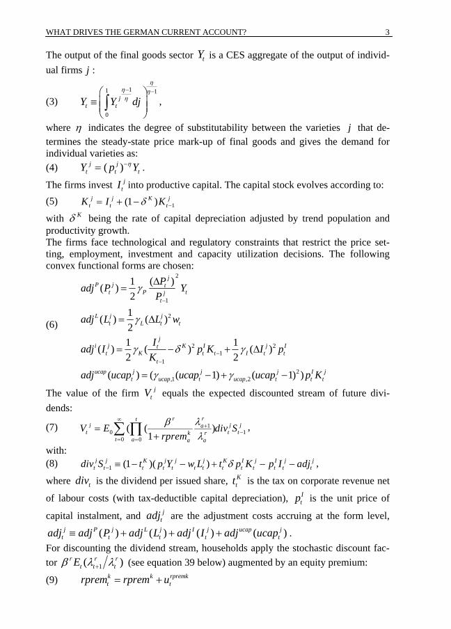
WHAT DRIVES THE GERMAN CURRENT ACCOUNT?

3

The output of the final goods sector tY is a CES aggregate of the output of individ-ual firms j :

(3) 11 1

0

jt tY Y dj

ηη ηη− −⎛ ⎞

≡ ⎜ ⎟⎜ ⎟⎝ ⎠∫ ,

where η indicates the degree of substitutability between the varieties j that de-termines the steady-state price mark-up of final goods and gives the demand for individual varieties as: (4) ( )j j

t t tY p Yη−= .

The firms invest jtI into productive capital. The capital stock evolves according to:

(5) 1(1 )j j K jt t tK I Kδ −= + −

with Kδ being the rate of capital depreciation adjusted by trend population and productivity growth. The firms face technological and regulatory constraints that restrict the price set-ting, employment, investment and capacity utilization decisions. The following convex functional forms are chosen:

(6)

2

1

2

2 21

12

,1 ,2

( )1( )21( ) ( )21 1( ) ( ) ( )2 2

( ) ( ( 1) ( 1) )

jP j t

t P tjt

L j jt L t t

ji j K I j It

t K t t I t tt

ucap j j j I jt ucap t ucap t t t

Padj P YP

adj L L w

Iadj I p K I pK

adj ucap ucap ucap p K

γ

γ

γ δ γ

γ γ

−

−−

Δ=

= Δ

= − + Δ

= − + −

The value of the firm jtV equals the expected discounted stream of future divi-

dends:

(7) 10 1

0 0

( ( )1

rrtj j ja

t t tk rt a a a

V E div Srprem

λβλ

∞+

−= =

=+∑ ∏ ,

with: (8) 1 (1 )( )j j K j j j K I j I j j

t t t t t t t t t t t t tdiv S t p Y w L t p K p I adjδ− ≡ − − + − − ,

where tdiv is the dividend per issued share, Ktt is the tax on corporate revenue net

of labour costs (with tax-deductible capital depreciation), Itp is the unit price of

capital instalment, and jtadj are the adjustment costs accruing at the form level,

( ) ( ) ( ) ( )j P j L j I j ucap jt t t t tadj adj P adj L adj I adj ucap≡ + + + .

For discounting the dividend stream, households apply the stochastic discount fac-tor 1( )r r r

t t tEβ λ λ+ (see equation 39 below) augmented by an equity premium:

(9) k k rpremkt trprem rprem u= +

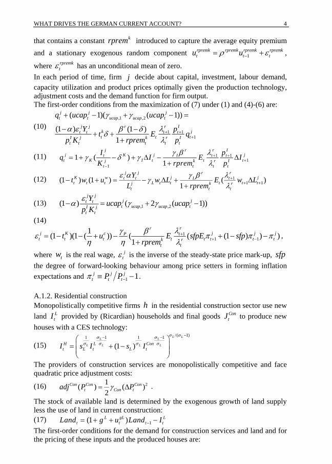
WHAT DRIVES THE GERMAN CURRENT ACCOUNT?

4

that contains a constant krprem introduced to capture the average equity premium and a stationary exogenous random component 1

rpremk rpremk rpremk rpremkt t tu uρ ε−= + ,

where rpremktε has an unconditional mean of zero.

In each period of time, firm j decide about capital, investment, labour demand, capacity utilization and product prices optimally given the production technology, adjustment costs and the demand function for firm output. The first-order conditions from the maximization of (7) under (1) and (4)-(6) are:

(10) ,1 ,2

1 11

( 1)( ( 1))

(1 ) (1 )1

j j jt t ucap ucap t

j j r Irk jt t t tt t tI j k r I

t t t t t

q ucap ucap

Y pt E qp K rprem p

γ γ

α ε λβ δδλ+ +

+

+ − + − =

− −+ +

+

(11) 1 11

1

1 ( )1

j r Irj K j jt t tI

t K I t t tj k r It t t t

I pq I E IK rprem p

λγ βγ δ γλ+ +

+−

= + − + Δ − Δ+

(12) 11 1(1 ) (1 ) ( )

1

j j rrK w j jt t tLt t t L t t t t tj k r

t t t

Yt w u w L E w LL rprem

ε α λγ βγλ+

+ +− + = − Δ + Δ+

(13) ,1 ,2(1 ) ( 2 ( 1))j j

j jt tt ucap ucap tI j

t t

Y ucap ucapp Kεα γ γ− = + −

(14)

11 1

1(1 )(1 ( )) ( ( (1 ) ) )1

rrj K j j jtP

t t t t t t t tk rt t

t u E sfpE sfprprem

ε λγ βε π π πη η λ

++ −= − − + − + − −

+,

where tw is the real wage, jtε is the inverse of the steady-state price mark-up, sfp

the degree of forward-looking behaviour among price setters in forming inflation expectations and 1 1j j j

t t tP Pπ −≡ − . A.1.2. Residential construction Monopolistically competitive firms h in the residential construction sector use new land L

tI provided by (Ricardian) households and final goods ContJ to produce new

houses with a CES technology:

(15) /( 1)1 11 1

(1 )L L

L L

L L L LH L Cont L t L tI s I s I

σ σσ σσ σ σ σ

−− −⎛ ⎞= + −⎜ ⎟⎜ ⎟⎝ ⎠

The providers of construction services are monopolistically competitive and face quadratic price adjustment costs:

(16) 21( ) ( )2

Con Con Cont Con tadj P Pγ= Δ .

The stock of available land is determined by the exogenous growth of land supply less the use of land in current construction: (17) 1(1 )L gL L

t t t tLand g u Land I−= + + − The first-order conditions for the demand for construction services and land and for the pricing of these inputs and the produced houses are:

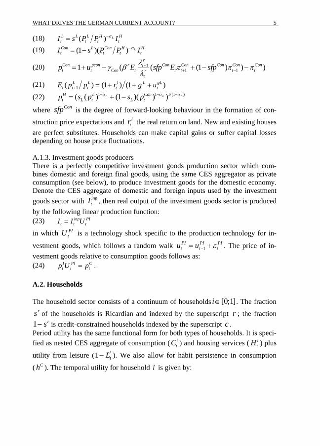
WHAT DRIVES THE GERMAN CURRENT ACCOUNT?

5

(18) ( ) LL L L H Ht t t tI s P P Iσ−=

(19) (1 )( ) LCon L Con H Ht t t tI s P P Iσ−= −

(20) 11 11 ( ( (1 ) ) )

rCon pcon r Con Con Con Con Contt t Con t t t t tr

t

p u E sfp E sfpλγ β π π πλ+

+ −= + − + − −

(21) 1( ) (1 ) (1 )L L l L gLt t t t tE p p r g u+ = + + +

(22) 1 1 1/(1 )( ( ) (1 )( ) )L L LH L Cont L t L tp s p s pσ σ σ− − −= + −

where Consfp is the degree of forward-looking behaviour in the formation of con-

struction price expectations and ltr the real return on land. New and existing houses

are perfect substitutes. Households can make capital gains or suffer capital losses depending on house price fluctuations. A.1.3. Investment goods producers There is a perfectly competitive investment goods production sector which com-bines domestic and foreign final goods, using the same CES aggregator as private consumption (see below), to produce investment goods for the domestic economy. Denote the CES aggregate of domestic and foreign inputs used by the investment goods sector with inp

tI , then real output of the investment goods sector is produced by the following linear production function: (23) inp PI

t t tI I U=

in which PItU is a technology shock specific to the production technology for in-

vestment goods, which follows a random walk 1PI PI PIt t tu u ε−= + . The price of in-

vestment goods relative to consumption goods follows as: (24) I PI C

t t tp U p= . A.2. Households The household sector consists of a continuum of households [0;1]i∈ . The fraction

rs of the households is Ricardian and indexed by the superscript r ; the fraction 1 rs− is credit-constrained households indexed by the superscript c . Period utility has the same functional form for both types of households. It is speci-fied as nested CES aggregate of consumption ( i

tC ) and housing services ( itH ) plus

utility from leisure (1 itL− ). We also allow for habit persistence in consumption

( Ch ). The temporal utility for household i is given by:

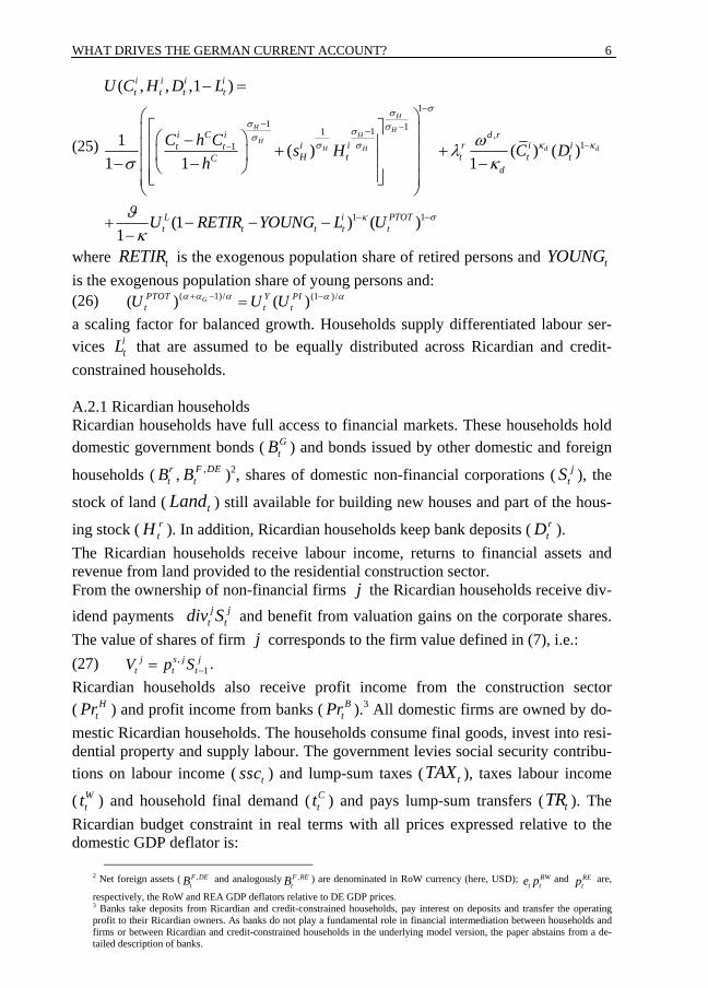
WHAT DRIVES THE GERMAN CURRENT ACCOUNT?

6

(25)

11 111 ,

11

1 1

( , , ,1 )

1 ( ) ( ) ( )1 1 1

(1 ) ( )1

HH H

HH

d dH H

i i i it t t t

i C i d ri i r i it tH t t t tC

d

L i PTOTt t t t t

U C H D L

C h C s H C Dh

U RETIR YOUNG L U

σσσ σσσ

κ κσ σ

κ σ

ωλσ κ

ϑκ

−

− −−−−

− −

− =

⎛ ⎞⎡ ⎤⎜ ⎟⎛ ⎞−⎢ ⎥⎜ ⎟+ +⎜ ⎟⎢ ⎥− − −⎜ ⎟⎝ ⎠⎢ ⎥⎣ ⎦⎜ ⎟⎝ ⎠

+ − − −−

where tRETIR is the exogenous population share of retired persons and tYOUNG is the exogenous population share of young persons and: (26) ( 1)/ (1 )/( ) ( )GPTOT Y PI

t t tU U Uα α α α α+ − −= a scaling factor for balanced growth. Households supply differentiated labour ser-vices i

tL that are assumed to be equally distributed across Ricardian and credit-constrained households. A.2.1 Ricardian households Ricardian households have full access to financial markets. These households hold domestic government bonds ( G

tB ) and bonds issued by other domestic and foreign

households ( rtB , ,F DE

tB )2, shares of domestic non-financial corporations ( jtS ), the

stock of land ( tLand ) still available for building new houses and part of the hous-

ing stock ( rtH ). In addition, Ricardian households keep bank deposits ( r

tD ). The Ricardian households receive labour income, returns to financial assets and revenue from land provided to the residential construction sector. From the ownership of non-financial firms j the Ricardian households receive div-idend payments j j

t tdiv S and benefit from valuation gains on the corporate shares. The value of shares of firm j corresponds to the firm value defined in (7), i.e.: (27) ,

1j s j j

t t tV p S −= . Ricardian households also receive profit income from the construction sector ( H

tPr ) and profit income from banks ( BtPr ).3 All domestic firms are owned by do-

mestic Ricardian households. The households consume final goods, invest into resi-dential property and supply labour. The government levies social security contribu-tions on labour income ( tssc ) and lump-sum taxes ( tTAX ), taxes labour income

( Wtt ) and household final demand ( C

tt ) and pays lump-sum transfers ( tTR ). The Ricardian budget constraint in real terms with all prices expressed relative to the domestic GDP deflator is:

2 Net foreign assets ( ,F DE

tB and analogously ,F REtB ) are denominated in RoW currency (here, USD); RW

t te p and REtp are,

respectively, the RoW and REA GDP deflators relative to DE GDP prices. 3 Banks take deposits from Ricardian and credit-constrained households, pay interest on deposits and transfer the operating profit to their Ricardian owners. As banks do not play a fundamental role in financial intermediation between households and firms or between Ricardian and credit-constrained households in the underlying model version, the paper abstains from a de-tailed description of banks.

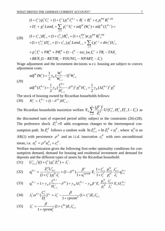
WHAT DRIVES THE GERMAN CURRENT ACCOUNT?

7

(28)

, ,

, ,

1

,1 1 1 1 1 1

, ,1 1 1 1

(1 ) (1 )

( ) ( )

(1 ) (1 ) (1 )

(1 ) (1 ) (

C C r C H H r r G RW F DEt t t t t t t t t t t

r L s j j W i H H rt t t t t t t

j

c r b G RW RW F DEt t t t t t t t

d r r l L s jt t t t t t

t p C t p I B B e p B

D p Land p S adj W adj I

r B r B r e p B

r D r p Land p di

=

− − − − − −

− − − −

+ + + + + +

+ + + + + =

+ + + + +

+ + + + + +

∑

11

,

)

(1 )

(1 )

j jt t

j

L L H B W i rt t t t t t t t t t

rt t t t t

v S

p I PR PR t ssc w L TR TAX

BEN RETIR YOUNG NPART L

−=

+ + + + − − + −

+ − − − −

∑

Wage adjustment and the investment decisions w.r.t. housing are subject to convex adjustment costs:

(29)

21

1,

, 2 , 21

1

1( ) ( 1)2

1 1( ) ( ) ( )2 2

iW i it

t W titH r

H H r H H r H r Htt H t t Ih t tr

t

Wadj W WW

Iadj I p H I pH

γ

γ δ γ

−−

−−

= −

= − + Δ

The stock of housing owned by Ricardian households follows: (30) ,

1(1 )r H r H rt t tH I Hδ −= + − .

The Ricardian households maximize welfare 00

( ) ( , , ,1 )r t

r r r rt t t t

t t

U C H D LZ β

β∞

=

Ε −∑ as

the discounted sum of expected period utility subject to the constraints (26)-(28). The preference shock 0tZ β > adds exogenous changes to the intertemporal con-

sumption path. ln tZ β follows a random walk 1ln lnt t tZ Z uβ β β+ = + , where tuβ is an

AR(1) with persistence βρ and an i.i.d. innovation tβε with zero unconditional

mean, i.e. 1t t tu uβ β β βρ ε−= + . Welfare maximization gives the following first-order optimality conditions for con-sumption demand, demand for housing and residential investment and demand for deposits and the different types of assets by the Ricardian household: (31) , ((1 ) )r C C r

C t t t t tU t p Z β λ+ = .

(32) ,, ,1 1 11

1(1 )(1 ) 1 1

r C H rrt H tH r H H rt t t

t t tC H r rpremh C H rt t t t t t t

Z U t pq E qt p u t p

β λβδλ λ

+ + ++

+= + −

+ + +

(33) ,

, , ,1 11

1

1 ( )H r H r

H r H H r r H rt t tt H Ih t Ih t t tr H r

t t t

I pq I E E IH p

λγ δ γ γ βλ

+ ++

−

= + − + Δ − Δ

(34) ,1( ) (1 )

1d

ir d r r c rtt t t t ti d

t

C r ED rprem

κ βλ ω λ λ += − ++

(35) 1(1 )1

r bn rt t t tb

t

r Erpremβλ λ += +

+

WHAT DRIVES THE GERMAN CURRENT ACCOUNT?

8

(36) 1 1(1 ) ( )1

r L L L rt t t t t tl

t

p r E prpremβλ λ+ += +

+

(37) 1 1 1, (1 ) ( )1

RW r RW RW rt t t t t t t te RW

t

e p r E e prpremβλ λ+ + += +

+

(38) , ,1 1 1(( ) )

1

rs j r s j j rt t t t t tk

t

p E p divrpremβλ λ+ + += +

+

where the rprem terms denote asset-specific risk premia. We define r

tr as the real (in terms of GDP prices) domestic interest rate without in-dividual asset risk. The risk-free rate and the stochastic discount factor are linked by: (39) 11 (1 ) ( )r r r r

t t t tr Eβ λ λ++ = Combining (39) with the asset specific returns in the (32)-(37) gives the following linear approximations for the asset-specific premia: (40) ,h r r rpremh

t t tr r u= + with 1

rpremh rpremh rpremh rpremht t tu uρ ε−= + and rpremh

tε as zero-mean exogenous shock,

(41) , ( / ) dd r d d r r rt t t tr r rprem C D κω= + − ,

where the constant drprem ensures correspondence to the risk-free interest rate in the steady state, (42) nb r b

t t tr r rprem= + where the risk premium on government bonds that are newly issued,

1

1

( )4

b b b tar rprembtt t

t

Brprem rprem by uY

ω −

−

≡ + − + , has an endogenous debt-dependent

element, and an exogenous AR(1) part 1rpremb rpremb rpremb rprembt t tu uρ ε−= + with the ze-

ro-mean i.i.d. innovation rprembtε . The endogenous component 1

1

( )4

b tart

t

B byY

ω −

−

− is

motivated by the empirical link between debt levels and bond returns and can be understood as heuristics adopted by households for the risk assessment; alterna-tively it could be derived from quadratic costs of deviating from target bond hold-ings. The average return on outstanding government debt in (28) is: (43) 1 (1 )( )b b b b r b

t t t tr r r rpremρ ρ−= + − + ,

where bρ accounts for the average maturity of government debt (see, e.g., Krause and Moyen (2013) for a model with multi-period debt). Up to a linear approximation, the equilibrium return on land obeys: (44) 1 1( )L r L l

t t t t t tr r E rpremπ π+ += − − + where we assume that the risk premium on land varies with the valuation of land compared to the steady-state value: ( )l l L L

t t t trprem rprem p Land Y val= − , and

where Lval is the value of land relative to GDP in the steady state.

WHAT DRIVES THE GERMAN CURRENT ACCOUNT?

9

The equilibrium condition w.r.t. to foreign bond holdings (37) implies (up to a first-order approximation): (45) , ,

1 1 1( ) ( )r RW RW DE EA EA RWt t t t t t t t t tr r E e e E rprem rpremπ π+ + += + Δ + − − −

where ,DE EAtrprem is the country risk premium of Germany relative to the EA ag-

gregate and ,EA RWtrprem is the risk premium of the EA aggregate relative to the

RoW. The endogenous part of the country risk premia depends on the relative NFA positions; we postulate , , ,( )DE EA e F DE F RE RW rpremde

t t t t trprem rprem B B Y u= − + and , , ,( )EA RW e F EA F RW RW rpremea

t t t t trprem rprem B B Y u= − + . The endogenous risk-premium response ensures stationarity of the NFA position (see, e.g., Kollmann, 2002); the exogenous components of the country risk premia,

1rpremde rpremde rpremde rpremdet t tu uρ ε−= + and 1

rpremea rpremea rpremea rpremeat t tu uρ ε−= + , are both

AR(1) processes with innovations rpremdetε and rpremea

tε respectively. An analogous condition holds for REA households: (46) , ,

1 1 1( ) ( )RE RW RW RE RE EA EA RWt t t t t t t t t tr r E e e E rprem rpremπ π+ + += + Δ + − − −

where we assume , , ,( )1

deRE EA e F RE F DE RW rpremret t t t tde

srprem rprem B B Y us

= − +−

,

with des being the economic size of Germany in the EA and rpremretu the ex-

ogenous AR(1) component 1rpremre rpremre rpremre rpremret t tu uρ ε−= + .

Applying the aggregation (1 )EA de r de REt t tr s r s r= + − gives for the aggregate EA:

(47) ,1 1 1( ) ( )EA RW RW EA EA RW

t t t t t t t t tr r E e e E rpremπ π+ + += + Δ + − − . Subtracting (47) from (45) and (46) we obtain expressions for intra-EA interest spreads:

(48) , ,

1 1( ) ( )F DE F RE

r EA EA e rpremdet tt t t t t tRW

t

B Br r E rprem uY

π π+ +

−= + − − +

(49) , ,

1 1( ) ( )1

F RE F DEdeRE EA EA RE e rpremret t

t t t t t tde RWt

B Bsr r E rprem us Y

π π+ +

−= + − − +

−.

The estimated model uses the EA and U.S. monetary policy rates for EAtr and RW

tr .

Hence, the real rate rtr for Germany equals the EA monetary policy rate plus the

German country risk premium from (48) and adjusted for inflation differentials. A.2.2 Credit constrained households Credit-constrained households differ from Ricardian households in two respects: they have a higher rate of time preference ( rc ββ < ), and they face a collateral con-straint on their borrowing. They borrow c

tB exclusively from domestic Ricardian households. The budget constraint of credit-constrained households in real terms with all prices expressed relative to the domestic GDP deflator is:

WHAT DRIVES THE GERMAN CURRENT ACCOUNT?

10

(50)

,1 1

,c ,1 1

(1 ) (1 ) (1 ) ( )

( ) (1 ) (1 )

(1 )

C C c C H H c c c c W it t t t t t t t t tH H c d c W i c

t t t t t t t t t t

ct t t t t

t p C t p I r B D adj W

adj I B TAX TR r D t ssc w L

BEN RETIR YOUNG NPART L

− −

− −

+ + + + + + +

+ = + + + + + − −

+ − − − −

with wage adjustment costs as in (28) and adjustment costs on housing investment:

(51) ,

,c 2 , 21

1

1 1( ) ( ) ( )2 2

H cH H H c H ct

t H t Ih tct

Iadj I H IH

γ δ γ−−

= − + Δ

The stock of housing owned by credit-constrained households evolves according to: (52) ,c

1(1 )c H H ct t tH I Hδ −= + −

The collateral constraint determines the borrowing capacity of the credit-constrained households: (53) , ,

1 1 1 1(1 ) (1 ) (1 ) ( (1 ))c c d c c c d c c H ct t t t t t t t tr B r B E p Hρ ρ χ π− − + ++ = + + − +

where the loan-to-value ratio that is imposed by Ricardian lenders is subject to a stochastic shock c c

t tuχχ χ= + . The credit-constrained households maximize welfare as the discounted sum of ex-

pected period utility 00

( ) ( ,1 , )c t

c c ct t t

t t

U C L HZ β

β∞

=

Ε −∑ subject to the constraints (50)-

(53). The first-order conditions for consumption and housing are:

(54) , 1,

1 1 1 1 ,

(1 (1 ) ) (1 )(1 )(1 ) (1 )

cc C CC tct t t t t

tc d c C C ct t t t t t C t

Ur t p ZEr E t p Z U

β

β

ψ βρ ψ

+

+ + + +

− + +=

+ − +

(55)

,c,c ,c

1,

1 1,

1

1 ( )

1 (1 ) ( )(1 )(1 )(1 )

HH H Htt H Ih tc

tc H H H c

t t t t t tIh rpremh c d c

t t t t

Iq IH

r E p p Iu r E

γ δ γ

ψγρ ψ

−

+ +

+

= + − + Δ

− + Δ−

+ + −

(56)

,,,

1,

,1 11, ,

1

(1 )1

(1 (1 ) )(1 ) (1 )(1 )(1 )(1 ) (1 )

cC d cH tH c c Ht t

t t t tH c Ct C t t

c H C HH ct t t t

t trpremh h c d c C Ht t t t t t

Upq Ep U t

r t pE qu r E t p

ρ ψ χ π

ψ δρ ψ

+

+ ++

+

−= +

+

− + − ++

+ + − +

where ctψ is the Lagrange multiplier of the collateral constraint. The interest rate for

collateral-constrained households is: (57) (1 )c d r d d

t t tr s r s r= − +

Furthermore we have ,h c c rpremht t tr r u= + and , ( / ) dd r d d c c c

t tr r rprem C D κω= + − , where the latter is analogous to (41) for Ricardian households and pins down the deposit holding by credit-constrained consumers. A.2.3 Wage setting

WHAT DRIVES THE GERMAN CURRENT ACCOUNT?

11

Trade unions are maximizing a joint utility function for each type of labour i . It is assumed that types of labour are distributed equally over Ricardian and credit-constrained households with their respective population weights. Nominal rigidity in wage setting is introduced in the form of adjustment costs for changing wages. The wage adjustment costs are borne by the household. The trade unions set wages by maximizing a weighted average of the utility func-tions of Ricardian and credit-constrained households. The wage rule is obtained by equating a weighted average of the marginal utility of leisure to a weighted average of the marginal utility of consumption times the real wage adjusted for a wage mark-up:

(58)

1 , 1 , 11 1 1 1

, ,

1

11

(1 ) 1( (1 ) ) ((1 )((1 ) ))(1 )

1(1 )((1 ) ) ( (1 ) )

( (1 ) ))

w w

r r r cL t L t C C W

t t t t t tr r r cC t C t

W WWt t t t t t t

rr WW t

t t t t trt

s U s Ut p t ssc w BEN

s U s U

t ssc w BEN w sfw

E w E sfw

ρ ρ

θ

γ π πθ θ

γ λβ π πθ λ

− − −− − − −

−

++

+ −+ − − − −

+ −

= − − − − + − −

− − −

The wage mark-up fluctuates around 1θ − , which is the inverse of the elasticity of substitution between different varieties of labour services. Fluctuation in the wage mark-up arises because of wage adjustment costs (27). Real benefits in GDP prices equal the replacement rate rimes the real wage: (59) U

t t tBEN b w= The ratio of the marginal utility of leisure to the marginal utility of consumption is a natural measure of the reservation wage. If the ratio is equal to the consumption wage net of benefit payments to non-working parts of the labour force, the house-hold is indifferent between, on the one hand, supplying an additional unit of labour and spending the additional income on consumption or, on the other hand, not in-creasing labour supply. The specification (58) also allows for real wage inertia wρ . Unit labour costs are

t t t tulc w L Y= , which equals the wage share in domestic income. A. 3 Trade and the current account In order to facilitate aggregation we assume that households, investment goods pro-ducers and the government have identical preferences across goods used for private consumption, public expenditure and investment. Let { }, , , ,, ,n i n i n i G nZ C I C∈ be

demand by an individual household, investment good producer or the government in country , ,n DE RE RW= . Then their preferences are given by the utility func-tion:

(60) 1 11 1

1, , , , , , , , ,(( ) ( ) (1 ) ( ) )n n nM M M

n n n n nM M M M Mn i d n M n d n i d n M n f n i

t t t t tZ s u Z s u Zσ σ σ

σ σ σ σ σ− −

−= − + − +

WHAT DRIVES THE GERMAN CURRENT ACCOUNT?

12

where , ,d n iZ and , ,f n iZ are indexes of demand across the continuum of differenti-ated goods produced in the domestic economy and abroad, respectively. The home bias parameter ,d ns can be subject to random shocks ,M n

tu . Households, firms and governments in country/region n have preferences over im-ports from country/region m given by

(61) 1 1

1

1 1

/( 1)11

, , , ,( )

n nn

n nf n n m f n m

mZ s Z

σ σσ

σ σ

−−⎛ ⎞

⎜ ⎟=⎜ ⎟⎝ ⎠∑

where , ,f n mZ are indexes of demand across the continuum of differentiated goods produced in exporting regions m , and ,n ms is the bilateral import share parameter. The elasticity parameters n

Mσ and 1nσ determine the price elasticity of bilateral

imports. In general we find that goods and services produced in Germany and the REA are closer substitutes to each other, while goods produced in the RoW are stronger complements to goods produced in the EA. This is reflected by

1 1, 1DE REσ σ < and by 1 1RWσ > and 1RWMσ < .

German exporters buy final domestic goods tX and transform them into exportable goods using a linear technology, so that export prices are given by:

(62) ,, , ,1 1

11 ( (1 ) ) / (1 )

X DEt PX x X DE x X DE X DE r

t Px t t t t t

pu sfp E sfp rγ π π π+ −

=− − + − − +

,

where PXtu is a price setting shock, Pxγ quantifies price adjustment costs and sfpx

is the degree of forward-looking in expectations. For the REA and the RoW we set 0PX

tu = and 0Pxγ = , so that the regions' export prices ,X RE REt tp p= and

,X RW RWt tp p= .

Importers buy foreign goods at quantity tM from foreign exporters and sell them on the domestic market, charging the domestic currency price:

(63) 1 1 11 1 1/(1 )

,

,

,

,

,

, ,1

, ,

1

(

1 ( (1 ) )1

( ) ( ) )DE DE DEDE RE

M DEt

P

X RE DE RW X RWt

M DE m M DE m M DE M DEPmt t t t t

t

t t

r

pu sf

s p s e

p

p

E sfpr

σ σ σ

γ π π π+ −

− − −

=− −

+

− + −+

,

where PMtu is a price setting shock, Pmγ quantifies price adjustment costs and

sfpm is the degree of forward-looking in expectations. For the REA and RoW we set 0PM

tu = and 0Pmγ = to obtain:

(64) 1 1 11 1 1

,/(1 ), , , ,

,

( ( ) ( ) )1

RE RE RERE DE X DE RE RW X RWtM RE

t PMt t

REt

s p spu

e pσ σ σ− − −

=−

+,

(65) 1 1 11 1 1/(1,

,), , ,

,

( ( ) ( ) )1

RW RW RWRW DE X DE RE RM RW

t PM R

W X W

W

R

t

t tt

s ppus pe

σ σ σ− − −

=−+

,

WHAT DRIVES THE GERMAN CURRENT ACCOUNT?

13

German import demand allows for some inertia in demand adjustment ( DEmγ ) and is

given by:

(66)

1, , 1

1 11 1 1

1 1

((1 )( ) )

DEm

DEDEmM

DEt

I Gt t

t t tC Ct t

M DEd DE M DE t t

t I GCt tt

t t tC Ct t

Mp pC I Gp p

p Ms up pp C I Gp p

γ

γσ −− −

− −− − −

− −

=+ +

⎛ ⎞⎜ ⎟⎜ ⎟− +⎜ ⎟

+ +⎜ ⎟⎝ ⎠

For REA and RoW imports we have analogous expressions:

(67) 1,

, , 1, , ,

1

(1 )( ) ( )

REm

REREmM

RE M RE REd RE M REt t t

td RE C RE d REt t t

M p Ms uY p Y

γγσ

−

− −

−

⎛ ⎞= − +⎜ ⎟⎝ ⎠

(68) 1,

, , 1, , ,

1

(1 )( ) ( )

RWm

RWRWmM

RW M RW RWd RW M RWt t t

td RW C RW d RWt t t

M p Ms uY p Y

γγσ

−

− −

−

⎛ ⎞= − +⎜ ⎟⎝ ⎠

where dtY is domestic demand in the REA and RoW, respectively, as defined be-

low. Exports of reach region are determined by the import demand of the other re-gions:

(69)

, ,

, ,

, ,

DE RE DE RW DEt t tRE DE RE RW REt t tRW DE RW RE RWt t t

X M M

X M M

X M M

= +

= +

= +

with bilateral import demand:

(70) 1

,,

,, ( )

DEX RE

DEttM DE

DE RE DE Rt

t

EM s p Mp

σ−=

(71) 1,,

,, ( )

DEX RW

DEt ttM DE

t

DE RW DE RWt

e pp

M s Mσ−=

(72) 1

,,

,, ( )

REX DE

REttM RE

RE DE RE Dt

t

EM s p Mp

σ−=

(73) 1,,

,, ( )

REX RW

t ttM

t

RE RW RE RW REt REM s e p M

pσ−=

(74) 1,

,,

, ( )RW

X DERWttM RW

t t

RW DE RW DEt tM p

e ps Mσ−=

(75) 1,

,,

, ( )RW

X REWt

tMRW RE RW RE RWt R

tW

t

pMp

s Me

σ−=

Consumer prices relative to the GDP deflator follow from (60) as: (76) 1 1/(1 ), , , ,((1 )( ) ( ))

DE DEM MC d DE M DE M d DE M DE Pc

t t t t tp s u p s u Uσ σ− −= − + + −

WHAT DRIVES THE GERMAN CURRENT ACCOUNT?

14

Real GDP in Germany equals the sum of its components: (77) ( )C G G I Con Con G

t t t t t t t t t t tY p C p C p I p I I TB= + + + + + ,

where , ,DE X DE DE M DE DEt t t t tTB p X p M≡ − is the trade balance in real (GDP price)

terms. The current account is the sum of net investment income from abroad, the trade bal-ance and the transfer account ( tTA ):

(78) ,1 1

DE RW RW F DE DE DEt t t t t t tCA r e p B TB TA− −≡ + +

The net international investment position (NIIP) equals the cumulated current ac-count plus valuation effects:

(79) ,

, , ,1 1(1 ) ( )

RW F DEt t t

RW RW F DE DE DE BWREV DE BW DEt t t t t t t t t

e p B

r e p B TB TA u u Y− −

=

+ + + + +.

Economy-wide real savings correspond to ( )DE I Con Con Gt t t t t t tS CA p I p I I≡ + + + .

A.4. Policy Government expenditure and receipts can deviate temporarily from their long-run levels in systematic response to budgetary or business-cycle conditions and in re-sponse to idiosyncratic shocks. Concerning government consumption and govern-ment investment, we specify the following autoregressive equations:

(80)

1 1

1

1

1

( ) ( )4

( )

G GG CG G B tart t t

LagPTOT PTOTt t t

DEF tar CGtt

t

C C BC C byU U Y

B def uY

τ τ

τ

− −

−

−

−

− = − − −

Δ− − +

(81) 1( )G G

G IG G IGt tLag tPTOT PTOT

t t

I II I uU U

τ −− = − +

Government consumption reacts to the level of government debt and the govern-ment deficit relative to the associated debt and deficit targets tarby and tardef . The price level of government consumption may deviate from private consumer prices by a stochastic shock C PG G

t t tp U p= . Government investment is considered to be predominantly infrastructure investment and is therefore priced at the construction price index. The transfer system consists of two parts, the benefit U

t tBEN b w= paid to the un-

employed members of the labour force (1 t t t tPENS YOUNG NPART L− − − − )

and other transfers tTR , including transfers to pensioners ( tPENS ). Unemployment

benefits and pensions are indexed to wages with replacement rates Utb and R

tb , with

1U U BUt t tb b u−= + and 1

R R BRt t tb b u−= + . Transfers may also react to the debt-to-GDP

ratio and the government deficit:

WHAT DRIVES THE GERMAN CURRENT ACCOUNT?

15

(82) 1 1

1 1

( ) ( )R G G

TRB tar TRDEF tar TRt t t t ttPTOT PTOT

t t t t

TR b w PENS B Bby def uU U Y Y

τ τ− −

− −

Δ= − − − − +

The stock of public capital, which enters the production function (1), evolves ac-cording to: (83) 1(1 )G G

t t tKG I KGδ −= + − .

Government revenue GtREV consists of taxes on consumption, labour and corpo-

rate income:

(84) ( )

( )

G C C C H H Wt t t t t t t t t t t

K K It t t t t t t

REV t p C t p I ssc t w L

t Y - w L - p K TAXδ

= + + +

+ +

with 1

C C tct t tt t u−= + and PTOT TAX

t t tTAX U U= . Labour income taxes follow a linear scheme, whereas labour income taxes are pro-gressive: (85) 0 1 1 2 3(1 ( 4 ))w w w

t t t t tt y y y y yτ τ − − −= + Δ + Δ + Δ + Δ − Δ 10

ww wt tt Y ττ=

with w0τ as the average tax rate and w

1τ as the degree of progressivity. The dynamics of government debt ( G

tB ) is given by:

(86) 1 1(1 ) (1 )G g Gt t t t t t t t

G G Con G Gt t t t t t

B r B BEN PENS YOUNG NPART L

TR p C p I REV− −= + + − − − −

+ + + −

The interest rate gtr is the implicit interest rate that the government pays on its debt.

It depends on the average maturity structure of sovereign debt (1 / (1 )gρ− ) and the rate b

tr on newly issued debt:

(87) 1 1(1 )g g g g b rprembt t t tr r r uρ ρ− −= + − +

Monetary policy is modelled by a Taylor rule where the ECB sets the policy rate

1EA EA EAt t t ti r E π +≡ + in response to area-wide inflation and real GDP growth. The

policy rate adjusts sluggishly to deviations of inflation and GDP growth from their respective target levels; the policy rule is also subject to random shocks:

(88)

, 3

0, , ,1 , 3

0

( )4

(1 )( )

4

M EAT EA Tt t i t

iEA M EA EA M EA i EAt lag t lag tM EA

y EAt i

i

ri i u

y y

πτπ π πτ τ

τ

−=

−

−=

⎛ ⎞+ + −⎜ ⎟

⎜ ⎟= + − +⎜ ⎟⎜ ⎟+ Δ −Δ⎜ ⎟⎝ ⎠

∑

∑

For the pre-EMU period we assume that monetary policy in the 'Euro Area' was conducted by the Bundesbank, which was setting the German policy rate, however, already targeting Euro aggregates. A.5. Equilibrium Equilibrium in the domestic model economy is an allocation by the price system and by government policies such that Ricardian and credit-constrained households

WHAT DRIVES THE GERMAN CURRENT ACCOUNT?

16

maximize utility, final goods producing firms, firms in the construction sector and investment goods producers maximize profits and markets clear. The market clearing for final domestic goods corresponds to (77): (89) , ,( )C I Con Con G G G X DE DE M DE DE

t t t t t t t t t t t t t tY p C p I p I I p C p X p M= + + + + + −

where total private consumption tC of domestic and imported goods is the sum of Ricardian and credit-constrained consumption as their per-capita consumption mul-tiplied by the respective population shares rs and 1 rs− : (90) (1 )r r r c

t t tC s C s C= + − . Similarly, total housing and construction investment are defined as: (91) , ,(1 )H r H r r H c

t t tI s I s I= + −

(92) , ,(1 )Con r Con r r Con ct t tI s I s I= + −

and equilibrium in the labour market is given by: (93) (1 )r r r c

t t tL s L s L= + − with r ct tL L= .

Credit-constrained households engage in debt contracts only with Ricardian house-holds, i.e.: (94) (1 )r c r r

t ts B s B− = . Total deposits are the population-weighted sum of Ricardian and credit-constrained deposits: (95) (1 )r r r c

t t tD s D s D= + − . A.6. REA and RoW blocks Rest of the euro area (REA) and rest of world (RoW) variables are denoted by su-perscripts RE and RW respectively. In order to identify demand and supply shocks in the REA and the RoW we use highly aggregated DSGE models with ag-gregate demand modelled by aggregate IS curves that do not distinguish between private and government demand:

(96) , , , ,

1, , ,1 1

REd RE C RE d RE RE

r t t tt d RE C RE d RE RE

t t t

Y h Y UEY h Y r

σ β

β −

+

⎛ ⎞−=⎜ ⎟− +⎝ ⎠

(97) , , , ,

1, , ,1 1

RWd RW C RW d RW RW

r t t tt d RW C RW d RW RW

t t t

Y h Y UEY h Y r

σ β

β −

+

⎛ ⎞−=⎜ ⎟− +⎝ ⎠

Firms' price setting is captured by a hybrid New Keynesian Phillips curve in which inflation rises in response to the region's output gap as the deviation of actual output from an exogenous stochastic trend:

(98) 1 1

, ,

1 ( (1 ) )1

(ln ln )

RE RE RE RE REt t t tRE

tRE RE T RE P RE

t t t

sfp E sfpr

Y Y u

π π π

ϕ

+ −

+−

= + −+

+

WHAT DRIVES THE GERMAN CURRENT ACCOUNT?

17

(99) 1 1

, ,

1 ( (1 ) )1

(ln ln )

RW RW RW RW RWt t t tRW

tRW RW T RW P RW

t t t

sfp E sfpr

Y Y u

π π π

ϕ

+ −

+−

= + −+

+

where trend output follows: (100) , , , ,

1 1 1ln ln (ln ln )T RE T RE Y RE RE DE TFP REt t t t tY Y Y Y uρ− − −= − − +

(101) , , , ,1 1 1ln ln (ln ln )T RW T RW Y RW RW DE TFP RW

t t t t tY Y Y Y uρ− − −= − − + GDP in the REA and the RoW equals domestic demand plus the trade balance: (102) , , , ,RE C RE d RE X RE RE M RE RE

t t t t t t tY p Y p X p M= + −

(103) , , , ,RW C RW d RW X RW RW M RW RWt t t t t t tY p Y p X p M= + −

The regions' consumer prices relative to the GDP price deflator are: (104) 1 1/(1 ), , , , , ,((1 )( ) ( ))

RE REM MC RE d RE M RE M RE d RE M RE

t t t tp s u p s uσ σ− −= − + + −

(105) 1 1/(1 ), , , , , ,((1 )( ) ( ))RW RWM MC RW d RW M RW M RW d RW M RW

t t t tp s u p s uσ σ− −= − + + − The REA NIIP position follows:

(106) , , ,1 1(1 )

RW RWF RE RW F RE RE RE BW RE REt t t tt t t t t t tRE RE

t t

e p e pB r B TB TA u Yp p− −= + + + +

where REtp and RW

tp are REA and RoW GDP process relative to the German GDP deflator. International goods and financial market clearing requires zero net trade and NFA positions at the global level, i.e. DE RE RE RW RW

t t t t t tTB p TB e p TB+ = − and , , ,F DE F RE F RW

t t tB B B+ = − . Interest rates in the REA are determined by (78) together with (38). RoW interest rates follow from the Taylor rule:

(107)

, 3

0, , ,1 , 3

0

( )4

(1 )( )

4

M RWT RW Tt t i t

iRW M RW RW M RW i RWt lag t lag tM RW

y RWt i

i

ri i u

y y

πτπ π πτ τ

τ

−=

−

−=

⎛ ⎞+ + −⎜ ⎟

⎜ ⎟= + − +⎜ ⎟⎜ ⎟+ Δ −Δ⎜ ⎟⎝ ⎠

∑

∑

with the RoW nominal and real rates linked by 1RW RW

ttRW

t tEr i π +−= .

WHAT DRIVES THE GERMAN CURRENT ACCOUNT?

18

B. Data description Data on GDP and its components, government finances, interest rates and external accounts for DE and the REA are from Eurostat (Quarterly National Accounts, Government Finance Statistics, and Balance of Payment Statistics). The data on DE house prices come from the ECB Statistical Warehouse. Quarterly data are season-ally adjusted. See Table B.1 for the list of variables observed in the estimation. The data are not de-trended, only divided by the German population trend. The construction of output, price, trade balance and interest rate series for the RoW and REA deserves more detail, which is provided below. B.1. RoW GDP volume and GDP deflator The data for RoW variables are constructed on the basis of data from 24 non-EA countries. The 24 countries are: Australia, Brazil, Bulgaria, Canada, China, Czech Republic, Denmark, Hong Kong, Hungary, Japan, Korea, Latvia, Lithuania, Mex-ico, New Zealand, Norway, Poland, Romania, Russia, Sweden, Switzerland, Tur-key, United Kingdom and United States. The data for GDP at current market prices and GDP at constant prices are taken from AMECO (Australia, Brazil, Canada, China, Hong Kong, Korea, Mexico, New Zealand and Russia) and Eurostat Quarterly National Accounts (all other countries) databases. The AMECO data are annual data that have been converted into quar-terly frequency. RoW (RW) nominal GDP is calculated as sum of nominal GDP for the 24 coun-tries, with nominal values converted into USD with E as the exchange rate of USD to national currency:

24

1RW i it t ti

YN E YN=

=∑

Given the currency transformation into USD, price inflation in the RoW is defined in USD terms and includes REER movements between the RoW members. The use of USD prices is consistent with using the Euro-USD exchange rate in trade equa-tions of the model and US interest rates in the RoW monetary policy rule. RoW nominal GDP is then normalised by its value in the base year t=0 (2005), giv-ing the index:

0 11

( )RW

tRW RW kt RWk

k

YNYN YNYN=

−

= ∏

To derive real GDP in the RoW, we first construct series for the 24 countries of GDP at constant domestic prices and normalise the series with GDP in the base year t=0 (2005):

0 11

( )i

ti i kt ik

k

YRYR YNYR=

−

= ∏

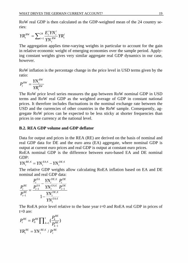
WHAT DRIVES THE GERMAN CURRENT ACCOUNT?

19

RoW real GDP is then calculated as the GDP-weighted mean of the 24 country se-ries:

∑ ==

24

1iitRW

t

it

itRW

t YRYN

YNEYR

The aggregation applies time-varying weights in particular to account for the gain in relative economic weight of emerging economies over the sample period. Apply-ing constant weights gives very similar aggregate real GDP dynamics in our case, however. RoW inflation is the percentage change in the price level in USD terms given by the ratio:

RWRW t

t RWt

YNPYR

=

The RoW price level series measures the gap between RoW nominal GDP in USD terms and RoW real GDP as the weighted average of GDP in constant national prices. It therefore includes fluctuations in the nominal exchange rate between the USD and the currencies of other countries in the RoW sample. Consequently, ag-gregate RoW prices can be expected to be less sticky at shorter frequencies than prices in one currency at the national level. B.2. REA GDP volume and GDP deflator Data for output and prices in the REA (RE) are derived on the basis of nominal and real GDP data for DE and the euro area (EA) aggregate, where nominal GDP is output at current euro prices and real GDP is output at constant euro prices. RoEA nominal GDP is the difference between euro-based EA and DE nominal GDP:

,€ ,€ ,€RE EA DEt t tYN YN YN= −

The relative GDP weights allow calculating RoEA inflation based on EA and DE nominal and real GDP data:

,€

,€1 1

,€1

,€1

EA DE DEt t t

RE EA EA DEt t t t

DEREttEAt

P YN PP P YN P

YNPYN

− −

−

−=

−

The RoEA price level relative to the base year t=0 and RoEA real GDP in prices of t=0 are:

0 11

( )RE

tRE RE kt REk

k

PP PP=

−

= ∏

REt

REt

REt PYNYR /,€=

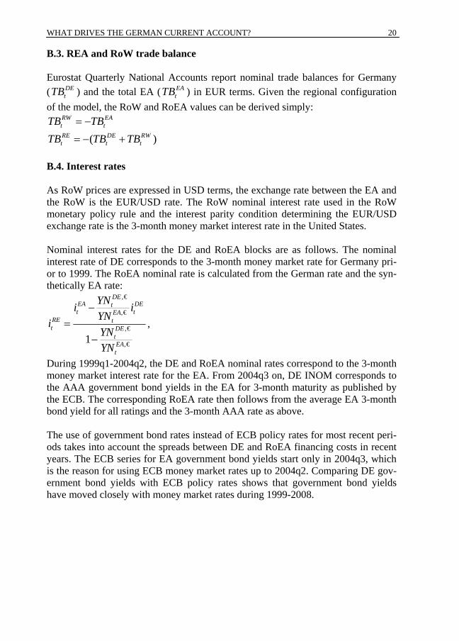
WHAT DRIVES THE GERMAN CURRENT ACCOUNT?

20

B.3. REA and RoW trade balance Eurostat Quarterly National Accounts report nominal trade balances for Germany ( DE

tTB ) and the total EA ( EAtTB ) in EUR terms. Given the regional configuration

of the model, the RoW and RoEA values can be derived simply: RW EAt tTB TB= −

( )RE DE RWt t tTB TB TB= − +

B.4. Interest rates As RoW prices are expressed in USD terms, the exchange rate between the EA and the RoW is the EUR/USD rate. The RoW nominal interest rate used in the RoW monetary policy rule and the interest parity condition determining the EUR/USD exchange rate is the 3-month money market interest rate in the United States. Nominal interest rates for the DE and RoEA blocks are as follows. The nominal interest rate of DE corresponds to the 3-month money market rate for Germany pri-or to 1999. The RoEA nominal rate is calculated from the German rate and the syn-thetically EA rate:

,€

,€

,€

,€1

DEEA DEtt tEA

RE tt DE

tEAt

YNi iYNiYNYN

−=

−,

During 1999q1-2004q2, the DE and RoEA nominal rates correspond to the 3-month money market interest rate for the EA. From 2004q3 on, DE INOM corresponds to the AAA government bond yields in the EA for 3-month maturity as published by the ECB. The corresponding RoEA rate then follows from the average EA 3-month bond yield for all ratings and the 3-month AAA rate as above. The use of government bond rates instead of ECB policy rates for most recent peri-ods takes into account the spreads between DE and RoEA financing costs in recent years. The ECB series for EA government bond yields start only in 2004q3, which is the reason for using ECB money market rates up to 2004q2. Comparing DE gov-ernment bond yields with ECB policy rates shows that government bond yields have moved closely with money market rates during 1999-2008.

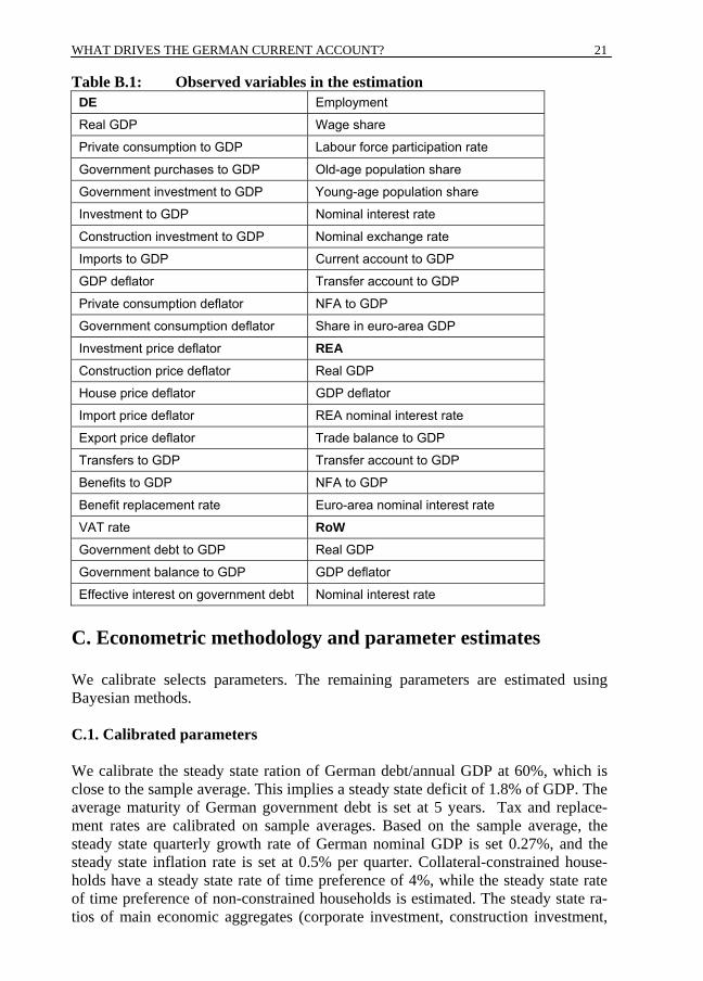
WHAT DRIVES THE GERMAN CURRENT ACCOUNT?

21

Table B.1: Observed variables in the estimation DE Employment

Real GDP Wage share

Private consumption to GDP Labour force participation rate

Government purchases to GDP Old-age population share

Government investment to GDP Young-age population share

Investment to GDP Nominal interest rate

Construction investment to GDP Nominal exchange rate

Imports to GDP Current account to GDP

GDP deflator Transfer account to GDP

Private consumption deflator NFA to GDP

Government consumption deflator Share in euro-area GDP

Investment price deflator REA Construction price deflator Real GDP

House price deflator GDP deflator

Import price deflator REA nominal interest rate

Export price deflator Trade balance to GDP

Transfers to GDP Transfer account to GDP

Benefits to GDP NFA to GDP

Benefit replacement rate Euro-area nominal interest rate

VAT rate RoW Government debt to GDP Real GDP

Government balance to GDP GDP deflator

Effective interest on government debt Nominal interest rate

C. Econometric methodology and parameter estimates We calibrate selects parameters. The remaining parameters are estimated using Bayesian methods. C.1. Calibrated parameters We calibrate the steady state ration of German debt/annual GDP at 60%, which is close to the sample average. This implies a steady state deficit of 1.8% of GDP. The average maturity of German government debt is set at 5 years. Tax and replace-ment rates are calibrated on sample averages. Based on the sample average, the steady state quarterly growth rate of German nominal GDP is set 0.27%, and the steady state inflation rate is set at 0.5% per quarter. Collateral-constrained house-holds have a steady state rate of time preference of 4%, while the steady state rate of time preference of non-constrained households is estimated. The steady state ra-tios of main economic aggregates (corporate investment, construction investment,

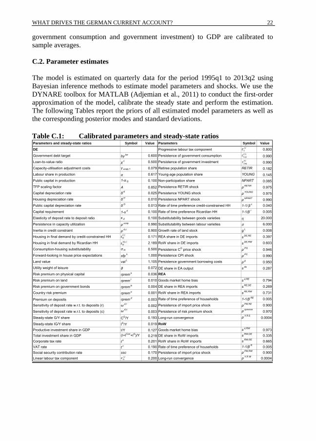
WHAT DRIVES THE GERMAN CURRENT ACCOUNT?

22

government consumption and government investment) to GDP are calibrated to sample averages. C.2. Parameter estimates The model is estimated on quarterly data for the period 1995q1 to 2013q2 using Bayesian inference methods to estimate model parameters and shocks. We use the DYNARE toolbox for MATLAB (Adjemian et al., 2011) to conduct the first-order approximation of the model, calibrate the steady state and perform the estimation. The following Tables report the priors of all estimated model parameters as well as the corresponding posterior modes and standard deviations. Table C.1: Calibrated parameters and steady-state ratios Parameters and steady-state ratios Symbol Value Parameters Symbol Value

DE Progressive labour tax component 0.800

Government debt target by tar 0.600 Persistence of government consumption 0.990Loan-to-value ratio χ c 0.500 Persistence of government investment 0.990Capacity-utilisation adjustment costs γ ucap,1 0.079 Retiree population share RETIR 0.182Labour share in production α 0.617 Young-age population share YOUNG 0.145Public capital in production 1-α G 0.100 Non-participation share NPART 0.085TFP scaling factor A 0.852 Persistence RETIR shock ρ RETIR 0.975Capital depreciation rate δ K 0.025 Persistence YOUNG shock ρ YOUNG 0.975Housing depreciation rate δ H 0.010 Persistence NPART shock ρ NPART 0.990Public capital depreciation rate δ G 0.013 Rate of time preference credit-constrained HH 1-1/ β c 0.040

Capital requirement 1-s d 0.100 Rate of time preference Ricardian HH 1-1/β r 0.005

Elasticity of deposit rate to deposit ratio κ d 0.100 Substitutability between goods varieties η 20.000

Persistence in capacity utilization ρ ucap 0.990 Substitutability between labour varieties θ 6.000

Inertia in credit constraint ρ d,c 0.900 Growth rate of land stock g L 0.008

Housing in final demand by credit-constrained HH 0.171 REA share in DE imports s DE,RE 0.397

Housing in final demand by Ricardian HH 2.189 RoW share in DE imports s DE,RW 0.603

Consumption-housing substitutability σ H 0.500 Persistence CG price shock ρ PG 0.946Forward-looking in house price expectations sfp h 1.000 Persistence CPI shock ρ PC 0.990Land value val L 1.105 Persistence government borrowing costs ρ g 0.950Utility weight of leisure ϑ 0.072 DE share in EA output s de 0.287Risk premium on physical capital rprem k 0.036 REA

Risk premium on land rprem l 0.010 Goods market home bias s d,RE 0.794

Risk premium on government bonds rprem b 0.004 DE share in REA imports s RE,DE 0.269

Country risk premium rprem e 0.001 RoW share in REA imports s RE,RW 0.731

Premium on deposits rprem d 0.003 Rate of time preference of households 1-1/β RE 0.005

Sensitivity of deposit rate w.r.t. to deposits (r) ω d,r 0.002 Persistence of import price shock ρ PM,RE 0.900

Sensitivity of deposit rate w.r.t. to deposits (c) ω d,c0.003 Persistence of risk premium shock ρ rpremre 0.970

Steady-state G/Y share CG/Y 0.193 Long-run convergence ρ Y,R E 0.0004

Steady-state IG/Y share IG/Y 0.019 RoWProductive investment share in GDP I/Y 0.127 Goods market home bias s d,RW 0.973Total investment share in GDP (I+ICon+IG)/Y 0.219 DE share in RoW imports s RW,DE 0.335Corporate tax rate t k 0.201 RoW share in RoW imports s RW,RE 0.665VAT rate t c 0.190 Rate of time preference of households 1-1/β R 0.005Social security contribution rate ssc 0.170 Persistence of import price shock ρ PM,RW 0.900Linear labour tax component 0.200 Long-run convergence ρ Y,R W 0.0004

NLCHs

CCHs

0wτ

1wτ

CGLagτIGLagτ

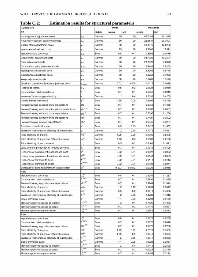
WHAT DRIVES THE GERMAN CURRENT ACCOUNT?

23

Table C.2: Estimation results for structural parameters Parameters

DE distrib mean std mode std

Housing stock adjustment costs γ H Gamma 30 20 65.0144 54.1448

Housing investment adjustment costs γ Ih Gamma 30 20 22.6681 20.3697

Capital stock adjustment costs γ K Gamma 30 20 23.4375 12.0232

Investment adjustment costs γ I Gamma 15 10 1.2041 1.2541

Import demand stickiness γ M Beta 0.8 0.1 0.8902 0.0476

Employment adjustment costs γ L Gamma 30 20 84.7026 19.3591

Price adjustment costs γ P Gamma 30 20 28.2326 7.6320

Construction price adjustment costs γ Con Gamma 30 20 2.4489 2.8263

Import price adjustment costs γ Pm Gamma 30 20 2.3066 0.9748

Export price adjustment costs γ Px Gamma 30 20 2.6252 3.1032

Wage adjustment costs γW Gamma 30 20 2.6761 1.3170

Quadratic capacity-utilisation adjustment costs γ ucap,2 Gamma 0.02 0.008 0.0115 0.0096

Real wage inertia ρ w Beta 0.5 0.2 0.9824 0.0050

Consumption habit persistence h c Beta 0.7 0.1 0.6955 0.0915

Inverse of labour supply elasticity κ Gamma 1 0.4 1.2133 0.4255

Goods market home bias s d Beta 0.65 0.06 0.6699 0.0138

Forward-looking in goods price expectations sfp Beta 0.7 0.1 0.9755 0.1365

Forward-looking in construction price expectations sfp Con Beta 0.7 0.1 0.8698 0.2467

Forward-looking in import price expectations sfp m Beta 0.7 0.1 0.7396 0.1268

Forward-looking in export price expectations sfp x Beta 0.7 0.1 0.7427 0.2622

Forward-looking in wage expectations sfw Beta 0.7 0.1 0.6946 0.3291

Ricardian household share s r Beta 0.5 0.15 0.5425 0.1832

Inverse of intertemporal elasticity of substitution σ Gamma 2 0.75 1.7378 0.4681

Price elasticity of imports Gamma 1.25 0.25 2.1089 0.5396

Price elasticity of imports of different sources Gamma 1.25 0.5 0.5100 2.2198

Price elasticity of land demand σ L Beta 0.5 0.2 0.6161 0.1871

Land share in production of housing services s L Beta 0.3 0.1 0.1049 0.0195

Response of government purchases to debt τ B Beta 0.02 0.01 0.0027 0.0022

Response of government purchases to deficit τ DEF Beta 0.02 0.01 0.0141 0.0069Response of transfers to debt τ TRB Beta 0.02 0.01 0.0111 0.0113Response of transfers to deficit τ TRDEF Beta 0.02 0.01 0.0123 0.0241Sensitivity of bond risk premium to public debt ω b Beta 0.003 0.0012 0.0025 0.0065REAImport demand stickiness Beta 0.8 0.1 0.5389 0.1283Consumption habit persistence h C,RE Beta 0.7 0.1 0.6691 0.1490Forward-looking in goods price expectations sfp RE Beta 0.7 0.1 0.9264 0.1824Price elasticity of imports Gamma 1.5 0.25 1.1299 0.5547Price elasticity of imports of different sources Gamma 0.5 0.2 0.6912 0.4308Inverse of intertemporal elasticity of substitution σ RE Gamma 2 0.75 2.4288 1.7918Slope of Phillips curve ϕ RE Gamma 1.1 0.05 1.0294 0.0169Monetary policy response to inflation Beta 2 0.4 1.7820 0.4228

Monetary policy response to output Beta 0.3 0.2 0.1446 0.0221Monetary policy rate persistence Beta 0.7 0.1 0.8849 0.0313RoWImport demand stickiness Beta 0.8 0.1 0.9325 0.0250Consumption habit persistence h C,RW Beta 0.7 0.1 0.8975 0.0448

Forward-looking in goods price expectations sfp RW Beta 0.7 0.1 0.8472 0.5706

Price elasticity of imports Gamma 1.25 0.25 0.7371 0.3309Price elasticity of imports of different sources Gamma 1.25 0.5 1.9641 1.0023Inverse of intertemporal elasticity of substitution σ RW Gamma 2 0.75 1.3947 0.6062Slope of Phillips curve ϕ RW Gamma 1.1 0.05 1.0026 0.0051Monetary policy response to inflation Beta 2 0.4 1.1419 0.2809Monetary policy response to output Beta 0.3 0.2 0.0022 0.0156Monetary policy rate persistence Beta 0.7 0.1 0.9458 0.0124

Prior Posterior

REMσ

,M EAlagτ

,M EAyτ

,M EAπτ

REmγ

RWmγ

,M RWlagτ

,M RWyτ

,M RWπτ

RWMσ

1REσ

DEMσ

1DEσ

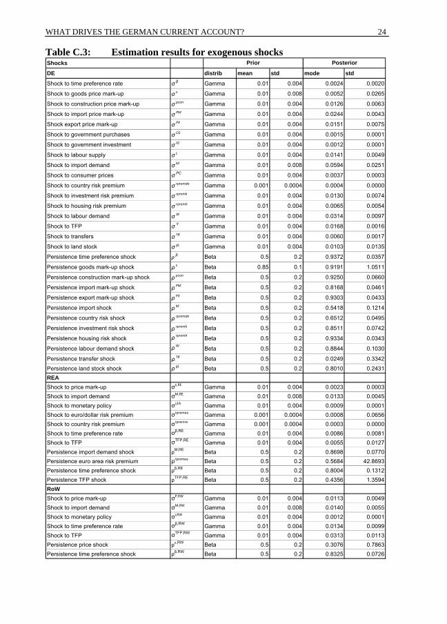
WHAT DRIVES THE GERMAN CURRENT ACCOUNT?

24

Table C.3: Estimation results for exogenous shocks Shocks

DE distrib mean std mode std

Shock to time preference rate σ β Gamma 0.01 0.004 0.0024 0.0020

Shock to goods price mark-up σ ε Gamma 0.01 0.008 0.0052 0.0265

Shock to construction price mark-up σ pcon Gamma 0.01 0.004 0.0126 0.0063

Shock to import price mark-up σ PM Gamma 0.01 0.004 0.0244 0.0043

Shock export price mark-up σ PX Gamma 0.01 0.004 0.0151 0.0075

Shock to government purchases σ CG Gamma 0.01 0.004 0.0015 0.0001

Shock to government investment σ IG Gamma 0.01 0.004 0.0012 0.0001

Shock to labour supply σ L Gamma 0.01 0.004 0.0141 0.0049

Shock to import demand σ M Gamma 0.01 0.008 0.0594 0.0251

Shock to consumer prices σ PC Gamma 0.01 0.004 0.0037 0.0003

Shock to country risk premium σ rpremde Gamma 0.001 0.0004 0.0004 0.0000

Shock to investment risk premium σ rpremk Gamma 0.01 0.004 0.0130 0.0074

Shock to housing risk premium σ rpremh Gamma 0.01 0.004 0.0065 0.0054

Shock to labour demand σW Gamma 0.01 0.004 0.0314 0.0097

Shock to TFP σ Y Gamma 0.01 0.004 0.0168 0.0016

Shock to transfers σ TR Gamma 0.01 0.004 0.0060 0.0017

Shock to land stock σ gL Gamma 0.01 0.004 0.0103 0.0135

Persistence time preference shock ρ β Beta 0.5 0.2 0.9372 0.0357

Persistence goods mark-up shock ρ ε Beta 0.85 0.1 0.9191 1.0511

Persistence construction mark-up shock ρ pcon Beta 0.5 0.2 0.9250 0.0660

Persistence import mark-up shock ρ PM Beta 0.5 0.2 0.8168 0.0461

Persistence export mark-up shock ρ PX Beta 0.5 0.2 0.9303 0.0433

Persistence import shock ρ M Beta 0.5 0.2 0.5418 0.1214

Persistence country risk shock ρ rpremde Beta 0.5 0.2 0.6512 0.0495

Persistence investment risk shock ρ rpremk Beta 0.5 0.2 0.8511 0.0742

Persistence housing risk shock ρ rpremh Beta 0.5 0.2 0.9334 0.0343

Persistence labour demand shock ρW Beta 0.5 0.2 0.8844 0.1030

Persistence transfer shock ρ TR Beta 0.5 0.2 0.0249 0.3342

Persistence land stock shock ρ gL Beta 0.5 0.2 0.8010 0.2431REAShock to price mark-up σε,RE Gamma 0.01 0.004 0.0023 0.0003Shock to import demand σM,RE Gamma 0.01 0.008 0.0133 0.0045Shock to monetary policy σi,EA Gamma 0.01 0.004 0.0009 0.0001Shock to euro/dollar risk premium σrpremea Gamma 0.001 0.0004 0.0008 0.0656Shock to country risk premium σrpremre Gamma 0.001 0.0004 0.0003 0.0000Shock to time preference rate σβ,RE Gamma 0.01 0.004 0.0086 0.0081Shock to TFP σTFP,RE Gamma 0.01 0.004 0.0055 0.0127Persistence import demand shock ρM,RE Beta 0.5 0.2 0.8698 0.0770Persistence euro area risk premium ρrpremea Beta 0.5 0.2 0.5684 42.8693Persistence time preference shock ρβ,RE Beta 0.5 0.2 0.8004 0.1312Persistence TFP shock ρTFP,RE Beta 0.5 0.2 0.4356 1.3594RoWShock to price mark-up σP,RW Gamma 0.01 0.004 0.0113 0.0049Shock to import demand σM,RW Gamma 0.01 0.008 0.0140 0.0055Shock to monetary policy σi,RW Gamma 0.01 0.004 0.0012 0.0001Shock to time preference rate σβ,RW Gamma 0.01 0.004 0.0134 0.0099Shock to TFP σTFP,RW Gamma 0.01 0.004 0.0313 0.0113Persistence price shock ρε,RW Beta 0.5 0.2 0.3076 0.7863Persistence time preference shock ρβ,RW Beta 0.5 0.2 0.8325 0.0726

Prior Posterior

WHAT DRIVES THE GERMAN CURRENT ACCOUNT?

25

Table C.4: Calibrated exogenous shocks Shocks Symbol Value

DE

Shock to unemployment benefit replacement rate σ BU 0.005

Shock to pension benefit replacement rate σ BR 0.005

Shock to RETIR shock σ RETIR 0.002

Shock to YOUNG σ YOUNG 0.002

Shock to NPART σ NPART 0.002

Shock to CG price σ PG 0.006Shock to government financing costs σ rpremb 0.000

Shock to consumption tax rate σ tc 0.002

Shock to lump-sum taxes σ TAX 0.015

Shock to transfer account σ TA,DE 0.010

Shock to NFA value σ BWREV,DE 0.050

NFA residual σ BW,DE 0.025

REA

Shock to transfer account σ TA,RE 0.050

Shock to NFA value σ BW,RE 0.040

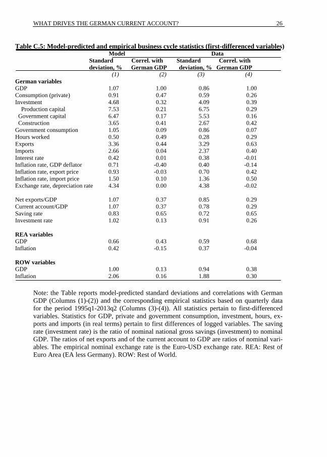
WHAT DRIVES THE GERMAN CURRENT ACCOUNT?

26

Table C.5: Model-predicted and empirical business cycle statistics (first-differenced variables) Model Data Standard Correl. with Standard Correl. with deviation, % German GDP deviation, % German GDP (1) (2) (3) (4) German variables GDP 1.07 1.00 0.86 1.00 Consumption (private) 0.91 0.47 0.59 0.26 Investment 4.68 0.32 4.09 0.39 Production capital 7.53 0.21 6.75 0.29 Government capital 6.47 0.17 5.53 0.16 Construction 3.65 0.41 2.67 0.42 Government consumption 1.05 0.09 0.86 0.07 Hours worked 0.50 0.49 0.28 0.29 Exports 3.36 0.44 3.29 0.63 Imports 2.66 0.04 2.37 0.40 Interest rate 0.42 0.01 0.38 -0.01 Inflation rate, GDP deflator 0.71 -0.40 0.40 -0.14 Inflation rate, export price 0.93 -0.03 0.70 0.42 Inflation rate, import price 1.50 0.10 1.36 0.50 Exchange rate, depreciation rate 4.34 0.00 4.38 -0.02 Net exports/GDP 1.07 0.37 0.85 0.29 Current account/GDP 1.07 0.37 0.78 0.29 Saving rate 0.83 0.65 0.72 0.65 Investment rate 1.02 0.13 0.91 0.26 REA variables GDP 0.66 0.43 0.59 0.68 Inflation 0.42 -0.15 0.37 -0.04 ROW variables GDP 1.00 0.13 0.94 0.38 Inflation 2.06 0.16 1.88 0.30

Note: the Table reports model-predicted standard deviations and correlations with German GDP (Columns (1)-(2)) and the corresponding empirical statistics based on quarterly data for the period 1995q1-2013q2 (Columns (3)-(4)). All statistics pertain to first-differenced variables. Statistics for GDP, private and government consumption, investment, hours, ex-ports and imports (in real terms) pertain to first differences of logged variables. The saving rate (investment rate) is the ratio of nominal national gross savings (investment) to nominal GDP. The ratios of net exports and of the current account to GDP are ratios of nominal vari-ables. The empirical nominal exchange rate is the Euro-USD exchange rate. REA: Rest of Euro Area (EA less Germany). ROW: Rest of World.

WHAT DRIVES THE GERMAN CURRENT ACCOUNT?

27

D. Sensitivity analysis Sensitivity analysis w.r.t. steady state (long-run) assumptions about German net for-eign assets (NFA) Table D.1: CA shock decomposition assuming steady state NFA equals 40% of annual GDP

1995 1996 1997 1998 1999 2000 2001 2002 2003 2004 2005 2006 2007 2008 2009 2010 2011 2012 2013 −0.1

−0.05

0

0.05

0.1

0.15quarter to quarter DE_CAY

TechnologyLabour wedgeUnemployment benefitRetireesPension replacement ratePrivate savingFiscal policyFirm finance wedgeHousing financing conditionsREA risk premiumExternal demand and tradeOthers

References (Appendix) Adjemian, S., H. Bastani, M. Juillard, F. Karamé, J. Maih, F. Mihoubi, G. Perendia, M. Ratto, and S. Villemot (2011): "DYNARE: Reference Manual, Version 4". DYNARE Working Paper 1. Krause, M., and S. Moyen (2013): "Public debt and changing inflation targets," Deutsche Bundesbank Discussion Papers 06/2013.