What Does Model-Driven Data AcquisitionReally Achieve in Wireless Sensor Networks?

Usman Raza∗†, Alessandro Camerra†, Amy L. Murphy∗, Themis Palpanas†, Gian Pietro Picco†∗ Center for Scientific and Technological Research, Bruno Kessler Foundation,Trento, Italy

{raza,murphy}@fbk.eu†Department of Information Engineering and Computer Science (DISI), University of Trento, Italy

{themis.palpanas,gianpietro.picco}@unitn.it

Abstract—Model-driven data acquisition techniques aim atreducing the amount of data reported, and therefore the energyconsumed, in wireless sensor networks (WSNs). At each node,a model predicts the sampled data; when the latter deviatefrom the current model, a new model is generated and sent tothe data sink. However, experiences in real-world deploymentshave not been reported in the literature. Evaluation typicallyfocuses solely on the quantity of data reports suppressed atsource nodes: the interplay between data modeling and theunderlying network protocols is not analyzed.

In contrast, this paper investigates in practice whetheri) model-driven data acquisition works in a real application;ii) the energy savings it enables in theory are still worthwhileonce the network stack is taken into account. We do so in theconcrete setting of a WSN-based system for adaptive lighting inroad tunnels. Our novel modeling technique, Derivative-BasedPrediction (DBP), suppresses up to 99% of the data reports,while meeting the error tolerance of our application. DBP isconsiderably simpler than competing techniques, yet performsbetter in our real setting. Experiments in both an indoortestbed and an operational road tunnel show also that, oncethe network stack is taken into consideration, DBP triples theWSN lifetime—a remarkable result per se, but a far cry fromthe aforementioned 99% data suppression. This suggests that,to fully exploit the energy savings enabled by data modelingtechniques, a coordinated operation of the data and networklayers is necessary.

I. INTRODUCTION

Wireless sensor networks (WSNs) provide the flexibilityof untethered sensing, but pose the challenge of achievingextended lifetime with a limited energy budget, often pro-vided by batteries. In this respect, it is well-known thatcommunication causes the biggest energy drain. This isunfortunate, given that the ability to report sensed data isthe one motivating the use of WSNs in several pervasivecomputing applications.

An approach to reduce communication without compro-mising data quality is to predict the trend followed bythe data being sensed. This technique is referred to asmodel-driven data acquisition and is applicable when data isreported periodically—the common case in many pervasivecomputing applications. In these cases, a model of the datatrend can be computed locally to a node, and constitutesthe information being reported to the data collection sink,

in place of several raw samples. As long as the locally-sensed data are compatible with the model prediction, nofurther communication is needed: only when the sensed datadeviates from the model, must the latter be updated and sentto the sink.

The aforementioned approach is well-known, and adoptedby several works we concisely survey in Section V. Never-theless, to the best of our knowledge none of these works hasbeen applied in a real-world pervasive application. There-fore, their practical applicability remains unascertained.Moreover, these works typically evaluate the gains only interms of messages suppressed w.r.t. a standard approachsending all samples. This data-centric view, however, isquite optimistic. WSN network protocols consume energynot only when transmitting and receiving data, but alsoin several continuous control operations, e.g., when main-taining a routing tree for data collection, or probing forongoing communication at the MAC layer. Therefore, thetrue question, currently unanswered by the literature, is towhat extent the theoretical savings enabled by model-drivendata acquisition are actually observable in practice when theapplication and network stack are combined.

Hence, in contrast with the existing literature, our goal is:• to investigate the benefits of model-driven data acqui-

sition in an existing deployment [1] providing closed-loop adaptive lighting in an operational road tunnel.As described in Section II, the WSN is used to pe-riodically report light samples, and is therefore repre-sentative of several pervasive computing applications,e.g., smart environments, building management, homeautomation [2];

• to assess the interplay of data modeling and the un-derlying network protocols, by evaluating qualitativelyand quantitatively the relationship between the two.

We achieve these goals with the following contributions:• we propose a novel method, called Derivative-Based

Prediction (DBP) for locally predicting the trendof data sensed by a WSN node. DBP, describedin Section III, is considerably simpler than existingmethods—a plus on resource-scarce WSN platforms.Nevertheless, our evaluation based on real-world data

�������������������� ������

�������������������������������������

������������������������������������

�����������������������������������������������������������������������

�����

�����

������������ ������

Figure 1. Physical placement of WSN nodes in the tunnel.

from the tunnel deployment shows that DBP performscomparably to existing techniques. As shown in Sec-tion IV, DBP suppresses up to 99% of the raw reportsin our application, while maintaining its data qualitywithin the required error tolerance.

• we analyze to what extent this staggering improvementis affected by the interaction with network protocols,by running our application on top of popular WSNprotocols (i.e., CTP [3] and Box-MAC [4]). Moreover,we feed the application the same light data “replayed”from the tunnel deployment, to directly compare thetheoretical gains against the practical ones. We do soin two settings: an operational tunnel, representative ofour target application, and a 40-node indoor testbed,representative of alternate application scenarios. Ourresults in Section IV confirm the expectation that thegains attained in practice when considering the networkstack are dramatically lower than those derived intheory by taking into account only the application mes-sages. However, the improvements are still remarkablein absolute terms: DBP triples the WSN lifetime w.r.t.a standard solution with periodic reporting.

Our results confirm that model-driven data acquisition canyield substantial lifetime improvements in practical settings.However, as we point out in the final remarks of Section VI,the results also suggest that, to fully exploit the energysavings made possible by model-driven data acquisition, co-ordination between the data and network layers is necessary.

II. WSN-BASED ADAPTIVE LIGHTING IN ROADTUNNELS

Our application case study is a WSN deployed in a roadtunnel to acquire light readings [1]. These are relayed inmulti-hop to a gateway, and from there to a ProgrammableLogic Controller (PLC) that closes the control loop bysetting the intensity of the lamps inside the tunnel. Incontrast with the state of the art in tunnels, where lightintensity is pre-set based on the current date and time, orat best determined by the external conditions, this closed-loop adaptive lighting system maintains optimal light levelsby considering the actual conditions inside the tunnel. Thisincreases safety, and enables considerable energy savings.

WSNs are an asset in this scenario, as the nodes canbe placed at arbitrary points along the tunnel, not only

where power and networking cables can reach. This drasti-cally reduces installation and maintenance costs, and makesWSNs particularly appealing for already existing tunnels,where changes to the infrastructure should be minimized.The downside to such flexibility is the reliance on anautonomous energy source. Nevertheless, battery costs areminimal and the replacement process can be easily combinedwith regularly-planned tunnel maintenance.

Figure 1 shows the placement of WSN nodes inside our260 m-long, two-way, two-lane tunnel. Overall, 40 nodesare split evenly between the tunnel walls and placed at aheight of 1.70 m, compatible with legal regulations. Theirdata reports are collected by a gateway, installed 2 m fromthe entrance. Each node is functionally equivalent to aTelosB mote [5], augmented with a sensor board equippedwith 4 ISL29004 digital light (illuminance) sensors. Thelight readings, collected at a sampling rate of 5 s, arelocally aggregated and filtered. Every 30 s, the result of thisaggregation is reported to the sink. The WSN nodes are nottime synchronized: a node reports its light value wheneverits 30 s timer expires.

This setup is similar to the one reported in [1], wherewe detail and evaluate the operational WSN-based, closed-loop adaptive lighting system. In this paper we use adifferent application and network stack, and compare ourmodel-driven data acquisition technique against the baselineconstituted by the aforementioned periodic reporting of allraw light samples.

III. DATA MODELING OF TIME SERIES WITH DBP

We define the data modeling problem we address in thispaper, and illustrate our novel DBP technique.

A. Problem Formulation

The application we described in Section II is an instanceof a general class of WSN applications where nodes periodi-cally take sensor measurements and report the correspondingsamples to a data sink. Moreover, we make the additionalassumption that the application running at the sink allowsfor a small tolerance in the accuracy of the reported data. Incontrast with the ideal requirements of the sink obtainingexact values in all data reports, the correctness of theseapplications is unaffected as long as i) the reported valuesmatch closely the exact ones; ii) inaccurate values occuronly occasionally. In other words, deviations from the exact

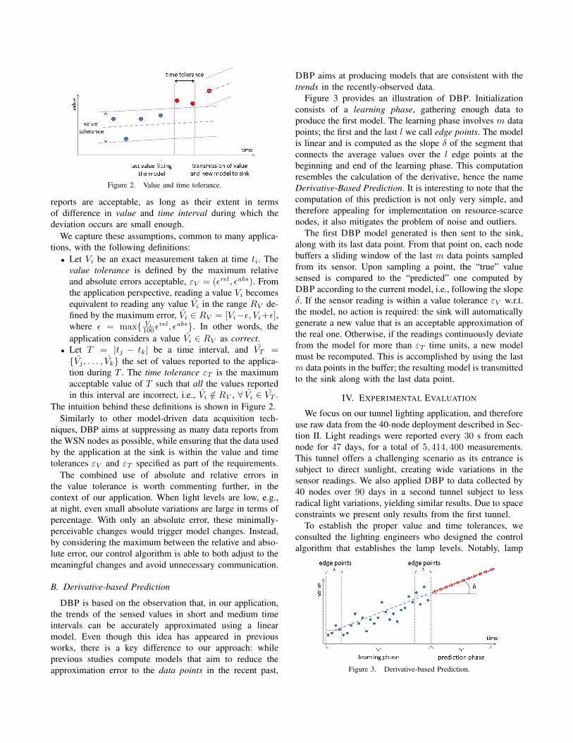
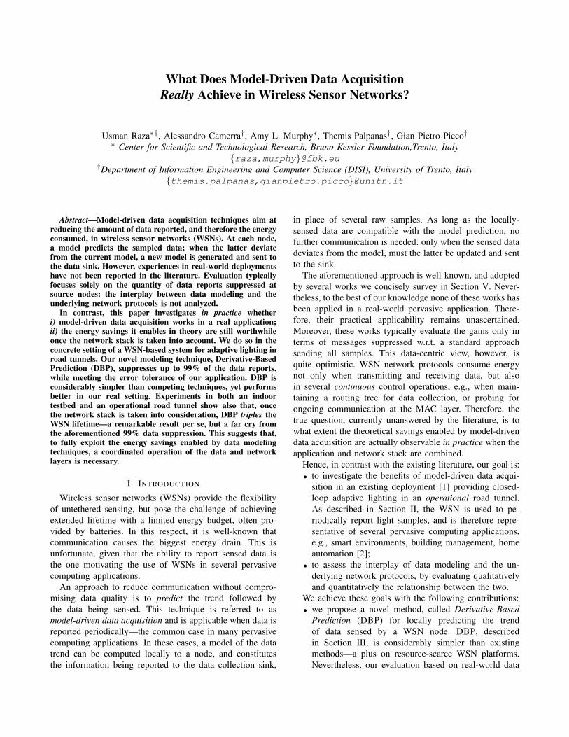
Figure 2. Value and time tolerance.

reports are acceptable, as long as their extent in termsof difference in value and time interval during which thedeviation occurs are small enough.

We capture these assumptions, common to many applica-tions, with the following definitions:

• Let Vi be an exact measurement taken at time ti. Thevalue tolerance is defined by the maximum relativeand absolute errors acceptable, εV = (εrel , εabs). Fromthe application perspective, reading a value Vi becomesequivalent to reading any value Vi in the range RV de-fined by the maximum error, Vi ∈ RV = [Vi−ε, Vi+ε],where ε = max{ Vi

100εrel , εabs}. In other words, the

application considers a value Vi ∈ RV as correct.• Let T = |tj − tk| be a time interval, and VT ={Vj , . . . , Vk} the set of values reported to the applica-tion during T . The time tolerance εT is the maximumacceptable value of T such that all the values reportedin this interval are incorrect, i.e., Vi /∈ RV , ∀ Vi ∈ VT .

The intuition behind these definitions is shown in Figure 2.Similarly to other model-driven data acquisition tech-

niques, DBP aims at suppressing as many data reports fromthe WSN nodes as possible, while ensuring that the data usedby the application at the sink is within the value and timetolerances εV and εT specified as part of the requirements.

The combined use of absolute and relative errors inthe value tolerance is worth commenting further, in thecontext of our application. When light levels are low, e.g.,at night, even small absolute variations are large in terms ofpercentage. With only an absolute error, these minimally-perceivable changes would trigger model changes. Instead,by considering the maximum between the relative and abso-lute error, our control algorithm is able to both adjust to themeaningful changes and avoid unnecessary communication.

B. Derivative-based Prediction

DBP is based on the observation that, in our application,the trends of the sensed values in short and medium timeintervals can be accurately approximated using a linearmodel. Even though this idea has appeared in previousworks, there is a key difference to our approach: whileprevious studies compute models that aim to reduce theapproximation error to the data points in the recent past,

DBP aims at producing models that are consistent with thetrends in the recently-observed data.

Figure 3 provides an illustration of DBP. Initializationconsists of a learning phase, gathering enough data toproduce the first model. The learning phase involves m datapoints; the first and the last l we call edge points. The modelis linear and is computed as the slope δ of the segment thatconnects the average values over the l edge points at thebeginning and end of the learning phase. This computationresembles the calculation of the derivative, hence the nameDerivative-Based Prediction. It is interesting to note that thecomputation of this prediction is not only very simple, andtherefore appealing for implementation on resource-scarcenodes, it also mitigates the problem of noise and outliers.

The first DBP model generated is then sent to the sink,along with its last data point. From that point on, each nodebuffers a sliding window of the last m data points sampledfrom its sensor. Upon sampling a point, the “true” valuesensed is compared to the “predicted” one computed byDBP according to the current model, i.e., following the slopeδ. If the sensor reading is within a value tolerance εV w.r.t.the model, no action is required: the sink will automaticallygenerate a new value that is an acceptable approximation ofthe real one. Otherwise, if the readings continuously deviatefrom the model for more than εT time units, a new modelmust be recomputed. This is accomplished by using the lastm data points in the buffer; the resulting model is transmittedto the sink along with the last data point.

IV. EXPERIMENTAL EVALUATION

We focus on our tunnel lighting application, and thereforeuse raw data from the 40-node deployment described in Sec-tion II. Light readings were reported every 30 s from eachnode for 47 days, for a total of 5, 414, 400 measurements.This tunnel offers a challenging scenario as its entrance issubject to direct sunlight, creating wide variations in thesensor readings. We also applied DBP to data collected by40 nodes over 90 days in a second tunnel subject to lessradical light variations, yielding similar results. Due to spaceconstraints we present only results from the first tunnel.

To establish the proper value and time tolerances, weconsulted the lighting engineers who designed the controlalgorithm that establishes the lamp levels. Notably, lamp

Figure 3. Derivative-based Prediction.

0

400

800

1200

1600

00:00 02:00 04:00 06:00 08:00 10:00 12:00 14:00 16:00 18:00 20:00 22:00 00:00

Lig

ht V

alu

e (

raw

)

Time

Actual Light ValueLight Value Predicted by DBP

Model Corrections by DBP

0

20

40

60

80

100

00:00 02:00 04:00 06:00 08:00 10:00 12:00 14:00 16:00 18:00 20:00 22:00 00:00

Err

or

Valu

e (

raw

)

Time

Value ToleranceAbsolute Error

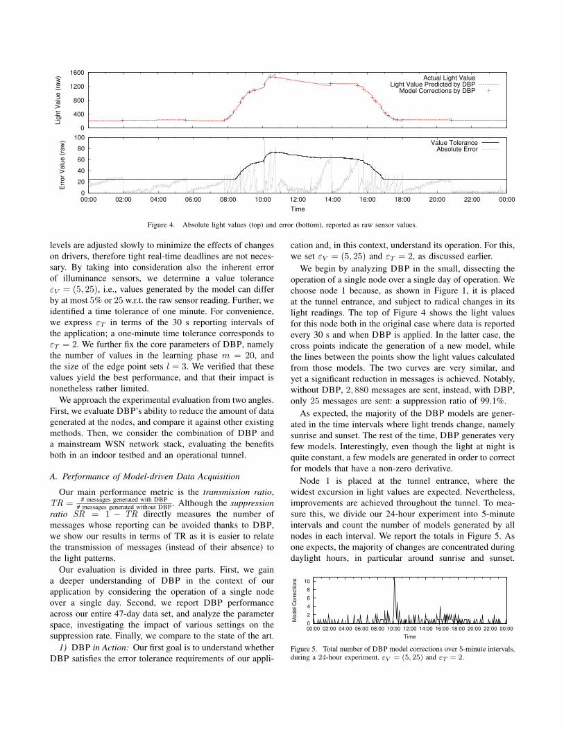
Figure 4. Absolute light values (top) and error (bottom), reported as raw sensor values.

levels are adjusted slowly to minimize the effects of changeson drivers, therefore tight real-time deadlines are not neces-sary. By taking into consideration also the inherent errorof illuminance sensors, we determine a value toleranceεV = (5, 25), i.e., values generated by the model can differby at most 5% or 25 w.r.t. the raw sensor reading. Further, weidentified a time tolerance of one minute. For convenience,we express εT in terms of the 30 s reporting intervals ofthe application; a one-minute time tolerance corresponds toεT = 2. We further fix the core parameters of DBP, namelythe number of values in the learning phase m = 20, andthe size of the edge point sets l = 3. We verified that thesevalues yield the best performance, and that their impact isnonetheless rather limited.

We approach the experimental evaluation from two angles.First, we evaluate DBP’s ability to reduce the amount of datagenerated at the nodes, and compare it against other existingmethods. Then, we consider the combination of DBP anda mainstream WSN network stack, evaluating the benefitsboth in an indoor testbed and an operational tunnel.

A. Performance of Model-driven Data Acquisition

Our main performance metric is the transmission ratio,TR = # messages generated with DBP

# messages generated without DBP . Although the suppressionratio SR = 1 − TR directly measures the number ofmessages whose reporting can be avoided thanks to DBP,we show our results in terms of TR as it is easier to relatethe transmission of messages (instead of their absence) tothe light patterns.

Our evaluation is divided in three parts. First, we gaina deeper understanding of DBP in the context of ourapplication by considering the operation of a single nodeover a single day. Second, we report DBP performanceacross our entire 47-day data set, and analyze the parameterspace, investigating the impact of various settings on thesuppression rate. Finally, we compare to the state of the art.

1) DBP in Action: Our first goal is to understand whetherDBP satisfies the error tolerance requirements of our appli-

cation and, in this context, understand its operation. For this,we set εV = (5, 25) and εT = 2, as discussed earlier.

We begin by analyzing DBP in the small, dissecting theoperation of a single node over a single day of operation. Wechoose node 1 because, as shown in Figure 1, it is placedat the tunnel entrance, and subject to radical changes in itslight readings. The top of Figure 4 shows the light valuesfor this node both in the original case where data is reportedevery 30 s and when DBP is applied. In the latter case, thecross points indicate the generation of a new model, whilethe lines between the points show the light values calculatedfrom those models. The two curves are very similar, andyet a significant reduction in messages is achieved. Notably,without DBP, 2, 880 messages are sent, instead, with DBP,only 25 messages are sent: a suppression ratio of 99.1%.

As expected, the majority of the DBP models are gener-ated in the time intervals where light trends change, namelysunrise and sunset. The rest of the time, DBP generates veryfew models. Interestingly, even though the light at night isquite constant, a few models are generated in order to correctfor models that have a non-zero derivative.

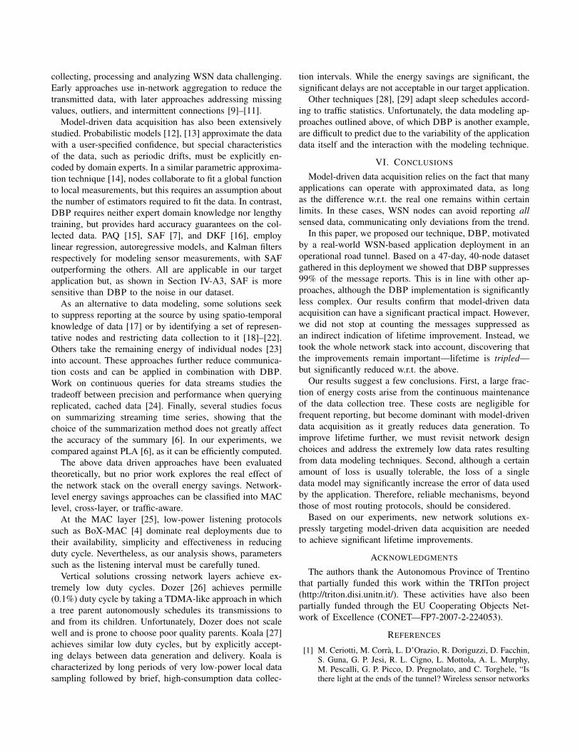
Node 1 is placed at the tunnel entrance, where thewidest excursion in light values are expected. Nevertheless,improvements are achieved throughout the tunnel. To mea-sure this, we divide our 24-hour experiment into 5-minuteintervals and count the number of models generated by allnodes in each interval. We report the totals in Figure 5. Asone expects, the majority of changes are concentrated duringdaylight hours, in particular around sunrise and sunset.

0

2

4

6

8

10

00:00 02:00 04:00 06:00 08:00 10:00 12:00 14:00 16:00 18:00 20:00 22:00 00:00

Model C

orr

ections

Time

Figure 5. Total number of DBP model corrections over 5-minute intervals,during a 24-hour experiment. εV = (5, 25) and εT = 2.

Nevertheless the total number of models in any 5-minuteinterval was below 10 and usually below 4. At night, thereare even fewer updates, with many intervals in which nomodels are generated.

Finally, in the bottom of Figure 4 we focus again onthe entrance node 1 as a representative example, to analyzethe error in the values provided by DBP to the applicationduring each 30 s reporting interval. The solid line indicatesthe value tolerance εV = (5, 25) set by our applicationrequirements, while the lighter line shows the error of DBPas the difference between the predicted value and the sensedraw value. In most cases, the error falls below the valuetolerance. Excursions above the value tolerance are causedby data predicted at the sink that, albeit incorrect, are withinthe time tolerance. In each of these cases, either subsequentvalues fell back below value tolerance or a new model wasgenerated after the maximum number of incorrect reports(εT = 2 in our case) was exceeded. Interestingly, at night,one can see the absolute error growing for a while, thendropping and growing again. The drop in error correspondsto the generation of a new model, visible also in the top ofFigure 4. The growing error is because the DBP model islinear with a small, but non-zero slope, which is slightly offthe measured light values that remain mostly constant.

2) Impact of Error Tolerance: The previous evaluationshows that DBP performs well for the requirements ofthe tunnel application. However, we want to explore theparameter space for DBP, to understand the effect ofchanges in the value and time tolerances on the transmissionratio. Figures 6(a)–6(c) show how TR changes at individualnodes for various combinations of parameters. Recall fromFigure 1 that nodes 1–20 are placed on the same North wall,while nodes 21–40 belong to the South wall. We plot a lineconnecting the TR at each node, because this best highlightsthe trends as one proceeds from the entrance to the interiorof the tunnel (e.g., from node 1 to 20 on the North wall).

In Figure 6(a) we vary the relative error εrel from 1%to 25%, keeping the absolute error constant εabs = 25. Bysetting the time tolerance to εT = 0, we force all deviationsfrom the value tolerances to be reported. To put these valuesin context, recall that the value tolerance εV is defined asthe maximum between the relative and absolute errors, εrel

and εabs . In Figure 6(b) we fix εrel = 5% and vary εabs

between 0 and 50, keeping εT = 0. In Figure 6(c), we usethe value tolerance εV = (5, 25) of our target applicationand vary εT between 0 and 4, i.e., from 0 to 2 minutes.

In all cases it is worth noting that, as expected, the biggestsavings are harvested from the nodes inside the tunnel, wherelight variations are rarer, and absolute values of illuminanceare smaller. Under these conditions, the linear nature of DBPaccurately models the linear nature of the data.

Interestingly, the trends seen for nodes 21-24 in Fig-ure 6(a) are due to the flickering of a light that introducednoise to the sensor readings. Nevertheless, even in this

case DBP achieved suppression ratios greater than 95%for these nodes. Further, in Figure 6(b), we clearly see theneed for both the absolute and relative value tolerances,as when the error tolerances are very low, e.g., εabs = 0or εabs = 10, TR is off the charts. This is because thelight sensors themselves have an error that often takes themoutside the small, fixed relative error εrel = 5%, triggeringunpredictable model changes. Further, the flickering lightintroduces additional noise that DBP cannot compensate forwith low error thresholds.

For each of these parameter combinations we also show,in Figure 6(d), the average TR over all nodes. An increasein the value of εrel brings a near linear reduction of TR.Instead, εabs and εT both achieve the greatest benefit at smallvalues, with diminishing returns as the value increases. Inthe former case, the reduction in TR progresses rapidly asεabs varies from 0 to 10, going from a suppression ratio of88% to 98%; a further (and larger) εabs increase from 10 to25 yields only an additional 2% reduction of TR. Similarly,time tolerance reflects the fact that changes in light valuesare gradual, and thus introducing even a small delay εT = 1

0

1

2

3

4

5

6

7

5 10 15 20

Tra

nsm

issio

n R

atio

x 1

00

Node ID

0

1

2

3

4

5

6

7

25 30 35 40

Tra

nsm

issio

n R

atio

x 1

00

Node ID

1%

3%

5%

10%

25%

(a) Relative error εrel (εabs = 25, εT = 0).

0

1

2

3

5 10 15 20

Tra

nsm

issio

n R

atio

x 1

00

Node ID

0

1

2

3

25 30 35 40

Tra

nsm

issio

n R

atio

x 1

00

Node ID

0

10

25

40

50

(b) Absolute error εabs (εrel = 5%, εT = 0).

0

1

2

3

5 10 15 20

Tra

nsm

issio

n R

atio

x 1

00

Node ID

0

1

2

3

25 30 35 40

Tra

nsm

issio

n R

atio

x 1

00

Node ID

0

1

2

3

4

(c) Time tolerance εT (εrel = 5%, εabs = 25).

0 0.1 0.2 0.3 0.4 0.5 0.6

0 5 10 15 20 25

Avg

. T

R x

100

εrel

2 4 6 8

10

0 10 20 30 40 50

Avg. T

R x

100

εabs

0 0.1 0.2 0.3 0.4 0.5 0.6

0 1 2 3 4

Avg. T

R x

100

εT

(d) Average transmission ratio for the combinations above.

Figure 6. Impact of error tolerance parameters on transmission ratio.

achieves most of the possible gain.In addition to the combinations in Figure 6, we also

computed the TR achieved with the strictest combination ofthe three parameters: εrel = 1%, εabs = 0, and εT = 0. Evenwith these worst-case requirements DBP still suppresses, onaverage, 63% of the reports. More interesting is the realcombination of parameters (εrel = 5%, εabs = 25, andεT = 2) suggested by the tunnel engineers, and used in therest of our experiments. In this case, the average suppressionrate is a staggering 99.7%—TR is reduced by almost twoorders of magnitude w.r.t. reporting all raw values. Theindividual TR achieved at each node is shown in Figure 7,where we compare DBP against state-of-the-art techniques,as discussed next.

3) Comparison to Other Approaches: We compared DBPagainst the following techniques, which in Section V are alsoput in the wider context of related work:

• Piecewise Linear Approximation (PLA) is a populartechnique that uses least square error linear segmentsto approximate a set of values [6]. In our case, eachnode uses a single segment to model for sensed values.

• Similarity-based Adaptable Framework (SAF) [7] relieson an autoregressive moving-average model of order 3with moving-average parameter of order 0. In SAF avalue Vi is predicted by a linear combination of thelast three: Vi = li + α1(Vi−1 − li−1) + α2(Vi−2 − li−2) +

α3(Vi−3 − li−3), where α1, α2, α3 are constants themodel must estimate, and li models the linear trend ofdata over time.

• As an additional point of comparison, we implementeda Polynomial Regression (POR) method. In contrast toDBP, POR allows the use of non-linear models for pre-diction. Intuitively, this may yield better performancethrough a better fit to the data. Like PLA, POR usesthe least squares measure for selecting the most ap-propriate coefficients for the polynomials, which havethe form y =

∑pk=0 αix

i. In this study, we evaluatedpolynomials of order p = 2, 3, 4. We used p = 2 as itprovides the best results for POR.

We used εV = (5, 25) and εT = 2, the requirements ofour target tunnel application. Table 7(a) shows the resultsw.r.t. the error in predicting the actual sensor readings.The values shown are the average error per point, over theentire 47-day dataset and over all nodes, computed as theEuclidean distance between the real sensed value and thevalue predicted by the corresponding model. We note thatPLA achieves a lower error than DBP. This is because DBPinherently permits some amount of error in the model, whilePLA employs an objective function that explicitly choosesthe model that minimizes the error. However, as we presentnext, DBP achieves a higher reduction in TR, because itbetter models the data trends.

In terms of communication performance, all approachesperform quite well, however, DBP achieves the best results,

as shown in Table 7(b) and Figure 7(c). As already men-tioned, DBP suppresses 99.7% of the message reports withour tunnel application requirements.

Because all approaches achieve very good results, it isworth noting that finding the derivative of the sensed data,at the core of DBP, is significantly less complex than solvinglinear equations with 2 or 3 unknowns, as required byPLA, POR and SAF. Notably, in our DBP implementation,used in the in-network evaluation explained in the followingsection, the core module to calculate the derivative containsonly 25 lines of TinyOS code, notably with no floatingpoint arithmetic. As node memory is limited, eliminatingthe floating point arithmetic module is greatly desirable.

Finally, in the course of our investigation, we stressedDBP by artificially modifying the data set, specificallyintroducing a significant amount of noise while maintainingthe trends. Notably, DBP was still able to achieve the bestsuppression ratios, even though the error of DBP was thelargest among the alternate approaches. This is due to thefact that the other approaches are designed to operate onrelatively smooth data, while DBP focuses on accuratelypredicting trends. The ability of DBP to achieve significantgains in the presence of noisy data can lead to a significantadvantage with other data sets. For example in the sametunnel project, we collected carbon monoxide (CO) data, andalthough the sampling period was lower (5 minutes insteadof 30 seconds), the noise in this data is significantly greater.Nevertheless, linear trends are present, as CO increasesduring the day when traffic is higher and decreases atnight. Therefore we expect DBP to perform quite well,significantly reducing the generated data.

B. Impact of the Network Stack

We study the performance of DBP in conjunction with thecommonly-used network stack composed of CTP [3], BoX-MAC [4], and TinyOS v2.1.1. We experiment in two set-tings: an operational road tunnel to evaluate DBP in the realconditions of our target application, and an indoor testbed,representative of scenarios with different connectivity.

DBP 0.00830PLA 0.00817SAF 0.00907POR 0.01900

(a) Average error.

DBP 0.00259PLA 0.00328SAF 0.00312POR 0.00712(b) Average TR.

0

1

2

3

4

5 10 15 20

Tra

nsm

issio

n R

atio

x 1

00

Node ID

0

1

2

3

4

25 30 35 40

Tra

nsm

issio

n R

atio

x 1

00

Node ID

DBP

PLA

SAF

POR

(c) Transmission ratio (TR) at individual nodes.

Figure 7. Comparing DBP to alternative approaches.

Tunnels are complex environments where factors suchas road traffic affect network behavior. For example, wepreviously observed [8] that in the presence of high traffic,nodes consistently select parents on their same side of thetunnel, while at low traffic nodes across the tunnel areoften selected. This is due to the interference caused byvehicles, nevertheless, it profoundly affects the shape andmaintenance cost of the routing tree. For these experiments,we relied on the 40-node WSN in Figure 1. The testbed iscomposed of 40 TelosB nodes in a 60x40 m2 office areashown in Figure IV-B. The node placement, along with thepower setting of −1 dBm, creates a network topology thatapproximately forms three segments, loosely reminiscent ofthe linear tunnel topology, but with larger diameter.

To assess directly the impact of the network stack onthe improvements theoretically attainable by DBP, we “re-played” the same data we used in Section IV-A both in thetunnel and testbed. As we could not re-execute the entire47-day dataset with multiple combinations of parameters,for the tunnel we selected a single 23-hour period, ensuringvariability in the vehicular traffic. Moreover, restrictionson the usage of the testbed forced us to run only 2-hourexperiments. Therefore, in this latter case we chose to focuson the sunrise period, the most challenging because valueschange dramatically and, unlike sunset, are not followed bythe night constant light levels. Figure 9 shows the numberof models generated by each node in both cases. We beginthe evaluation after DBP has been initialized, specificallyafter generation and transmission of the first model.

We now study how data delivery to the application,network lifetime, and routing costs are affected by DBP.All of these aspects, and particularly the first two, are deeplyaffected by the operation of the MAC layer, specifically therate at which the radio duty cycles, which therefore becomesa key parameter in our experiments. At low sleep intervals,nodes frequently check the channel but find no activity,increasing idle listening costs. At large sleep intervals, thecost to transmit a packet increases. In BoX-MAC, trans-mission to a non-sink node takes on average half the sleepinterval, due to the fact that the sender must transmit until the

Figure 8. Testbed map and connectivity.

0

2

4

6

8

10

12

14

16

18

0 5 10 15 20 25 30 35 40

Nu

mb

er

of

Mo

de

l M

essa

ge

s

Node ID

(a) Testbed: TR = 0.0048, 2 hours.

0

10

20

30

40

50

60

0 5 10 15 20 25 30 35 40

Nu

mb

er

of

Mo

de

l M

essa

ge

s

Node ID

(b) Tunnel: TR = 0.0014, 23 hours.

Figure 9. Number of model update messages.

receiver wakes up, receives the packet, then acknowledges itsreception [4]. This long transmission interval also increasesthe probability of packet collisions among hidden terminals,further decreasing the delivery ratio and increasing energyconsumption. The ideal sleep interval balances idle listeningand active transmission costs. To identify the best interval forour application, we ran experiments with a range of valuesfrom 500 to 3000 ms.

1) Data Delivery: DBP greatly reduces the amount ofdata in the network w.r.t. the baseline where all nodes senddata every 30 s. The reduction in data transmitted reducesthe probability of collisions, therefore increasing the deliveryratio. This is evident in Figure 10, where the system withDBP loses fewer messages than without DBP. In all casesthe delivery is very good, above 97%, but DBP actuallyachieves 100% in all cases and in both scenarios, except forthe case with the maximum sleep interval of 3000 ms inthe testbed. In this case, a single model message was lost;however, as the absolute number of model changes is small,the total delivery ratio drops by almost 3%. Although thisloss rate may be acceptable without DBP, losing a singleDBP model has the potential to introduce large errors at thesink, as the latter will continue to predict sensor values withan out-of-date model until the next one is received. Thissuggests that, based on the target environment or parametersettings, dedicated mechanisms may be required to ensurereliability of model transmissions.

2) Lifetime: To study the impact on lifetime, we measurethe duty cycle of the radio. Indeed, as this is the mostpower-hungry component, the time spent in communicationactivities is the most significant factor contributing to thesystem lifetime. Figure 11 clearly shows that DBP enables

97

97.5

98

98.5

99

99.5

100

500 1000 1500 2000 2500 3000

Deliv

ery

Ratio (

%)

Sleep Interval (ms)

Without DBPWith DBP

(a) Testbed (2 hours).

99.8

99.9

100

500 1000 1500 2000 2500 3000

Deliv

ery

Ratio (

%)

Sleep Interval (ms)

Without DBPWith DBP

(b) Tunnel (23 hours).

Figure 10. Delivery ratio.

0

2

4

6

8

10

500 1000 1500 2000 2500 3000

Ave

rag

e D

uty

Cycle

(%

)

Sleep Interval (ms)

Without DBPWith DBP

Only CTP

(a) Testbed (2 hours).

0

1

2

3

4

5

500 1000 1500 2000 2500 3000

Ave

rag

e D

uty

Cycle

(%

)

Sleep Interval (ms)

Without DBPWith DBP

Only CTP

(b) Tunnel (23 hours).

Figure 11. Average duty cycle. The y-axis scale is different.

significant savings at any sleep interval. Indeed, the bestsleep interval, corresponding to the lowest duty cycle, is1500 ms without DBP. Further increasing the sleep intervaldecreases the idle listening cost, but it increases the trans-mission cost as the average transmission duration is half thesleep interval. This phenomenon instead bears a negligibleeffect in DBP where transmissions are greatly reduced. Inthis case, longer sleep intervals can be used to increaselifetime without affecting data delivery.

Figure 11(a) shows that in the testbed, with a sleep intervalof 1500 ms (i.e., the best without DBP), DBP yields morethan twice the lifetime of the no-DBP baseline—i.e., theWSN running DBP lasts twice as long, with the sameMAC settings. Using the best sleep interval in both cases(i.e., 1500 and 3000 ms, respectively) yields a three-foldlifetime improvement. The energy savings in the tunnel, inFigure 11(b), are less remarkable although still significant.The network diameter in the tunnel is much smaller w.r.t.the testbed, due to the waveguide effect described in [8];many direct, 1-hop links to the sink exist, leaving less roomfor improvement.

0

2

4

6

8

10

500 1000 1500 2000 2500 3000

Ave

rag

e D

uty

Cycle

(%

)

Sleep Interval (ms)

Multiple HopsSingle Hop

Figure 12. Tunnel: duty cycle by distanceto the gateway, no DBP.

The impact of1-hop links tothe sink is worthcommenting further.Indeed, because thesink is always on,it quickly receivesand acknowledgesa packet, makingtransmissions fromits direct children very short and therefore low-energy. Thiscan be seen clearly in Figure 12 where, for the tunnelexperiments, we measure separately the duty cycle of thenodes that spent their entire lifetime directly connectedto the sink and those that, at any time, were more thanone hop away. Directly-connected nodes enjoy much lowerenergy costs. The plot considers only the case withoutDBP. Interestingly, with DBP all the nodes reportingmodel changes (Figure 9(b)) where in direct range of thesink. Indeed, as shown in Figure 1, the latter is attached tothe gateway placed at the entrance, where light variations,and hence model changes, occur. This placement was notour deliberate choice, as it was originally determined by

0

1000

2000

3000

4000

5000

6000

0 5 10 15 20 25 30 35 40

Lin

k L

evel T

Xs

Node ID

CTP BeaconsMsg TXs

Forwarded Msg TXsRetransmissions

(a) Without DBP.

0

50

100

150

200

250

0 5 10 15 20 25 30 35 40

Lin

k L

evel T

Xs

Node ID

CTP BeaconsMsg TXs

Forwarded Msg TXsRetransmissions

(b) With DBP.

Figure 13. Tunnel: total link-level transmissions for a sleep interval of1500 ms. The y-axis scale is different.

the available power panels in the tunnel. Nevertheless, ithints at the fact that, if a priori application knowledgeis available about the sensors that are likely to generatethe most variations, this can be exploited by a consequentplacement of the gateway. A similar optimization is notpossible without DBP, as all nodes must send data.

3) Routing Costs: A natural question arises at this point:if DBP suppresses over 99% of the messages, why does thenetwork lifetime increase “only” three-fold? This is due tothe costs of the network stack, in particular the idle listeningand average transmission times of the MAC protocol, and tothe overhead of the routing protocol to build and maintainthe data collection tree. As we already evaluated the impactof the MAC layer, here we turn to the routing layer.

To isolate the inherent costs (e.g., tree maintenance)of CTP, we ran experiments with no application traffic.The corresponding duty cycle is shown as Only CTP inFigure 11; interestingly, the DBP cost is very close tothe cost of CTP tree maintenance, regardless of the sleepinterval. A finer-grained view is provided by Figure 13,where we analyze the different components of traffic in thenetwork. Without DBP, the dominate component is messagetransmission and forwarding; significant retransmissions arepresent for some nodes, while the component ascribed toCTP (i.e., the beacons probing for link quality) is negli-gible. When DBP is active, the number of CTP beaconsremains basically unchanged. However, because application-level traffic is dramatically reduced, CTP beacons becomethe dominant component of network traffic.

In conclusion, these last observations highlight that furtherreductions in data traffic would have little practical impacton the system lifetime, as routing costs are dominated bytopology maintenance rather than data forwarding. Further,applying alternate data modeling techniques, e.g., PLA, SAFand POR, will not have a significant effect on systemlifetime, as they cannot reduce these fixed, routing costs.Therefore, improvements are more likely to come fromradical changes at the routing and MAC layers, taking intoaccount the traffic patterns of model-driven data acquisition.

V. RELATED WORK

The limited resources, variable connectivity, and spatio-temporal correlation among sensed values make efficiently

collecting, processing and analyzing WSN data challenging.Early approaches use in-network aggregation to reduce thetransmitted data, with later approaches addressing missingvalues, outliers, and intermittent connections [9]–[11].

Model-driven data acquisition has also been extensivelystudied. Probabilistic models [12], [13] approximate the datawith a user-specified confidence, but special characteristicsof the data, such as periodic drifts, must be explicitly en-coded by domain experts. In a similar parametric approxima-tion technique [14], nodes collaborate to fit a global functionto local measurements, but this requires an assumption aboutthe number of estimators required to fit the data. In contrast,DBP requires neither expert domain knowledge nor lengthytraining, but provides hard accuracy guarantees on the col-lected data. PAQ [15], SAF [7], and DKF [16], employlinear regression, autoregressive models, and Kalman filtersrespectively for modeling sensor measurements, with SAFoutperforming the others. All are applicable in our targetapplication but, as shown in Section IV-A3, SAF is moresensitive than DBP to the noise in our dataset.

As an alternative to data modeling, some solutions seekto suppress reporting at the source by using spatio-temporalknowledge of data [17] or by identifying a set of represen-tative nodes and restricting data collection to it [18]–[22].Others take the remaining energy of individual nodes [23]into account. These approaches further reduce communica-tion costs and can be applied in combination with DBP.Work on continuous queries for data streams studies thetradeoff between precision and performance when queryingreplicated, cached data [24]. Finally, several studies focuson summarizing streaming time series, showing that thechoice of the summarization method does not greatly affectthe accuracy of the summary [6]. In our experiments, wecompared against PLA [6], as it can be efficiently computed.

The above data driven approaches have been evaluatedtheoretically, but no prior work explores the real effect ofthe network stack on the overall energy savings. Network-level energy savings approaches can be classified into MAClevel, cross-layer, or traffic-aware.

At the MAC layer [25], low-power listening protocolssuch as BoX-MAC [4] dominate real deployments due totheir availability, simplicity and effectiveness in reducingduty cycle. Nevertheless, as our analysis shows, parameterssuch as the listening interval must be carefully tuned.

Vertical solutions crossing network layers achieve ex-tremely low duty cycles. Dozer [26] achieves permille(0.1%) duty cycle by taking a TDMA-like approach in whicha tree parent autonomously schedules its transmissions toand from its children. Unfortunately, Dozer does not scalewell and is prone to choose poor quality parents. Koala [27]achieves similar low duty cycles, but by explicitly accept-ing delays between data generation and delivery. Koala ischaracterized by long periods of very low-power local datasampling followed by brief, high-consumption data collec-

tion intervals. While the energy savings are significant, thesignificant delays are not acceptable in our target application.

Other techniques [28], [29] adapt sleep schedules accord-ing to traffic statistics. Unfortunately, the data modeling ap-proaches outlined above, of which DBP is another example,are difficult to predict due to the variability of the applicationdata itself and the interaction with the modeling technique.

VI. CONCLUSIONS

Model-driven data acquisition relies on the fact that manyapplications can operate with approximated data, as longas the difference w.r.t. the real one remains within certainlimits. In these cases, WSN nodes can avoid reporting allsensed data, communicating only deviations from the trend.

In this paper, we proposed our technique, DBP, motivatedby a real-world WSN-based application deployment in anoperational road tunnel. Based on a 47-day, 40-node datasetgathered in this deployment we showed that DBP suppresses99% of the message reports. This is in line with other ap-proaches, although the DBP implementation is significantlyless complex. Our results confirm that model-driven dataacquisition can have a significant practical impact. However,we did not stop at counting the messages suppressed asan indirect indication of lifetime improvement. Instead, wetook the whole network stack into account, discovering thatthe improvements remain important—lifetime is tripled—but significantly reduced w.r.t. the above.

Our results suggest a few conclusions. First, a large frac-tion of energy costs arise from the continuous maintenanceof the data collection tree. These costs are negligible forfrequent reporting, but become dominant with model-drivendata acquisition as it greatly reduces data generation. Toimprove lifetime further, we must revisit network designchoices and address the extremely low data rates resultingfrom data modeling techniques. Second, although a certainamount of loss is usually tolerable, the loss of a singledata model may significantly increase the error of data usedby the application. Therefore, reliable mechanisms, beyondthose of most routing protocols, should be considered.

Based on our experiments, new network solutions ex-pressly targeting model-driven data acquisition are neededto achieve significant lifetime improvements.

ACKNOWLEDGMENTS

The authors thank the Autonomous Province of Trentinothat partially funded this work within the TRITon project(http://triton.disi.unitn.it/). These activities have also beenpartially funded through the EU Cooperating Objects Net-work of Excellence (CONET—FP7-2007-2-224053).

REFERENCES

[1] M. Ceriotti, M. Corra, L. D’Orazio, R. Doriguzzi, D. Facchin,S. Guna, G. P. Jesi, R. L. Cigno, L. Mottola, A. L. Murphy,M. Pescalli, G. P. Picco, D. Pregnolato, and C. Torghele, “Isthere light at the ends of the tunnel? Wireless sensor networks

for adaptive lighting in road tunnels,” in Proc. of the Int. Conf.on Information Processing in Sensor Networks (IPSN), 2011.

[2] J. A. Stankovic, I. Lee, A. Mok, and R. Rajkumar, “Op-portunities and obligations for physical computing systems,”Computer, vol. 38, 2005.

[3] O. Gnawali, R. Fonseca, K. Jamieson, D. Moss, and P. Levis,“The collection tree protocol,” in Proc. of the Int. Conf. onEmbedded Networked Sensor Systems (SenSys), 2009.

[4] D. Moss and P. Levis, “BoX-MACs: Exploiting Physical andLink Layer Boundaries in Low-Power Networking,” Tech.Rep. SING-08-00, 2008.

[5] J. Polastre, R. Szewczyk, and D. Culler, “Telos: Enablingultra-low power wireless research,” in Proc. of the Int. Conf.on Information Processing in Sensor Networks (IPSN), 2005.

[6] T. Palpanas, M. Vlachos, E. J. Keogh, and D. Gunopulos,“Streaming time series summarization using user-defined am-nesic functions,” IEEE Trans. on Knowledge Data Engineer-ing, vol. 20, no. 7, 2008.

[7] D. Tulone and S. Madden, “An energy-efficient queryingframework in sensor networks for detecting node similari-ties,” in Proc. of the Int. Conf. on Modeling, Analysis andSimulation of Wireless and Mobile Systems (MSWiM), 2006.

[8] L. Mottola, G. Picco, M. Ceriotti, S. Guna, and A. Murphy,“Not All Wireless Sensor Networks Are Created Equal: AComparative Study On Tunnels.” ACM Trans. on SensorNetworks (TOSN), vol. 7, no. 2, 2010.

[9] L. Gruenwald, M. S. Sadik, R. Shukla, and H. Yang, “DEMS:a data mining based technique to handle missing data inmobile sensor network applications,” in Proc. of the Int. Conf.on Data Mgmt. for Sensor Networks (DMSN), 2010.

[10] A. Deligiannakis, Y. Kotidis, V. Vassalos, V. Stoumpos, andA. Delis, “Another outlier bites the dust: Computing meaning-ful aggregates in sensor networks,” in Proc. of the Int. Conf.on Data Eng. (ICDE), 2009.

[11] W. Wu, H.-B. Lim, and K.-L. Tan, “Query-driven data collec-tion and data forwarding in intermittently connected mobilesensor networks,” in Proc. of Int. Conf. on Data Mgmt. forSensor Networks (DMSN), 2010.

[12] A. Deshpande, C. Guestrin, S. Madden, J. M. Hellerstein, andW. Hong, “Model-driven data acquisition in sensor networks,”in Proc. of the Int. Conf. on Very Large Data Bases (VLDB),2004.

[13] D. Chu, A. Deshpande, J. M. Hellerstein, and W. Hong,“Approximate data collection in sensor networks using prob-abilistic models,” in Proc. of the Int. Conf. on Data Eng.(ICDE), 2006.

[14] C. Guestrin, P. Bodik, R. Thibaux, M. Paskin, and S. Madden,“Distributed regression: an efficient framework for modelingsensor network data,” in Proc. of the Int. Symp. on Informa-tion Processing in Sensor Networks (IPSN), 2004.

[15] D. Tulone and S. Madden, “PAQ: Time series forecastingfor approximate query answering in sensor networks,” inProceedings of the European Wkshp. on Wireless SensorNetworks (EWSN), 2006.

[16] A. Jain, E. Y. Chang, and Y.-F. Wang, “Adaptive streamresource management using Kalman filters,” in Proc. of theInt. Conf. on Management of Data (SIGMOD), 2004.

[17] A. Silberstein, G. Filpus, K. Munagala, and J. Y. 0001, “Data-driven processing in sensor networks,” in Proc. of the Conf.on Innovative Data Systems Research (CIDR), 2007.

[18] Y. Kotidis, “Snapshot queries: Towards data-centric sensornetworks,” in Proc. of the Int. Conf. on Data Eng. (ICDE),2005.

[19] Z. Zhou, S. Das, and H. Gupta, “Connected k-coverageproblem in sensor networks,” in Proc. of the Int. Conf. onComputer Communications and Networks (IC3N), 2004.

[20] M. C. Vuran, O. B. Akan, and I. F. Akyildiz, “Spatio-temporal correlation: theory and applications for wirelesssensor networks,” Computer Networks, vol. 45, no. 3, 2004.

[21] H. Jiang, S. Jin, and C. Wang, “Prediction or not? An energy-efficient framework for clustering-based data collection inwireless sensor networks,” IEEE Trans. on Parallel Dis-tributed Systems, vol. 22, June 2011.

[22] M. Hassani, E. Mller, P. Spaus, A. Faqolli, T. Palpanas, andT. Seidl, “Self-organizing energy aware clustering of nodesin sensor networks using relevant attributes,” in Proc. ofthe Int. Wkshp. on Kowledge Discovery from Sensor Data(SensorKDD), 2010.

[23] R. A. F. Mini, M. D. V. Machado, A. A. F. Loureiro, andB. Nath, “Prediction-based energy map for wireless sensornetworks,” Ad Hoc Networks, vol. 3, 2005.

[24] C. Olston, J. Jiang, and J. Widom, “Adaptive filters forcontinuous queries over distributed data streams,” in Proc.of the Int. Conf. on Management of Data (SIGMOD), 2003.

[25] J. Rousselot, A. El-Hoiydi, and J.-D. Decotignie, “Lowpower medium access control protocols for wireless sensornetworks,” in Proc. of the European Wireless Conf. (EW),June 2008.

[26] N. Burri, P. von Rickenbach, and R. Wattenhofer, “Dozer:ultra-low power data gathering in sensor networks,” in Proc.of the Int. Conf. on Information processing in sensor networks(IPSN), 2007.

[27] R. Musaloiu-E., C.-J. M. Liang, and A. Terzis, “Koala: Ultra-low power data retrieval in wireless sensor networks,” in Proc.of the Int. Conf. on Information processing in sensor networks(IPSN), 2008.

[28] X. Ning and C. G. Cassandras, “Dynamic sleep time controlin wireless sensor networks,” ACM Trans. on Sensor Net-works, vol. 6, June 2010.

[29] C. J. Merlin and W. B. Heinzelman, “Duty cycle control forlow power listening mac protocols,” in Proc. of the Int. Conf.on Mobile Ad-hoc and Sensor Systems (MASS), 2008.