Work ing PaPer Ser ieSno 1522 / march 2013

What doeS a financial Shock do?

firSt international evidence

Fabio Fornari and Livio Stracca

In 2013 all ECB publications

feature a motif taken from

the €5 banknote.

note: This Working Paper should not be reported as representing the views of the European Central Bank (ECB). The views expressed are those of the authors and do not necessarily reflect those of the ECB.

macroPrudential reSearch netWork

© European Central Bank, 2013

Address Kaiserstrasse 29, 60311 Frankfurt am Main, GermanyPostal address Postfach 16 03 19, 60066 Frankfurt am Main, GermanyTelephone +49 69 1344 0Internet http://www.ecb.europa.euFax +49 69 1344 6000

All rights reserved.

ISSN 1725-2806 (online)EU Catalogue No QB-AR-13-019-EN-N (online)

Any reproduction, publication and reprint in the form of a different publication, whether printed or produced electronically, in whole or in part, is permitted only with the explicit written authorisation of the ECB or the authors.

This paper can be downloaded without charge from http://www.ecb.europa.eu or from the Social Science Research Network electronic library at http://ssrn.com/abstract_id=2224062.

Information on all of the papers published in the ECB Working Paper Series can be found on the ECB’s website, http://www.ecb.europa.eu/pub/scientific/wps/date/html/index.en.html

Macroprudential Research NetworkThis paper presents research conducted within the Macroprudential Research Network (MaRs). The network is composed of economists from the European System of Central Banks (ESCB), i.e. the 27 national central banks of the European Union (EU) and the European Central Bank. The objective of MaRs is to develop core conceptual frameworks, models and/or tools supporting macro-prudential supervision in the EU.

The research is carried out in three work streams: 1) Macro-financial models linking financial stability and the performance of the economy; 2) Early warning systems and systemic risk indicators; 3) Assessing contagion risks.

MaRs is chaired by Philipp Hartmann (ECB). Paolo Angelini (Banca d’Italia), Laurent Clerc (Banque de France), Carsten Detken (ECB), Simone Manganelli (ECB) and Katerina Šmídková (Czech National Bank) are workstream coordinators. Javier Suarez (Center for Monetary and Financial Studies) and Hans Degryse (Katholieke Universiteit Leuven and Tilburg University) act as external consultant. Fiorella De Fiore (ECB) and Kalin Nikolov (ECB) share responsibility for the MaRs Secretariat.

The refereeing process of this paper has been coordinated by a team composed of Gerhard Rünstler , Kalin Nikolov and Bernd Schwaab (all ECB).

The paper is released in order to make the research of MaRs generally available, in preliminary form, to encourage comments and suggestions prior to final publication. The views expressed in the paper are the ones of the author(s) and do not necessarily reflect those of the ECB or of the ESCB.

AcknowledgementsWe thank participants in a seminar at the ECB for useful comments, in particular A. Calza, M. Lenza, A. Musso and B. Winkler, as well as participants in the Economic Policy Panel in Budapest, 15 April 2011, in particular our discussants Michael Haliassos and Refet Gürkaynak. We also thank 3 referees for their very useful suggestions. The views expressed in the paper belong to the authors and are not necessarily shared by the ECB.

Fabio FornariEuropean Central Bank; e-mail: fabio.fornari@ecb.europa.eu

Livio Stracca (corresponding author)European Central Bank; e-mail: livio.stracca@ecb.europa.eu

Lamfalussy Fellowships

This paper has been produced under the ECB Lamfalussy Fellowship programme. This programme was launched in 2003 in the context of the ECB-CFS Research Network on “Capital Markets and Financial Integration in Europe”. It aims at stimulating high-quality research on the structure, integration and performance of the European financial system.

The Fellowship programme is named after Baron Alexandre Lamfalussy, the first President of the European Monetary Institute. Mr Lamfalussy is one of the leading central bankers of his time and one of the main supporters of a single capital market within the European Union.

Each year the programme sponsors five young scholars conducting a research project in the priority areas of the Network. The Lamfalussy Fellows and their projects are chosen by a selection committee composed of Eurosystem experts and academic scholars. Further information about the Network can be found at http://www.eufinancial-system.org and about the Fellowship programme under the menu point “fellowships”.

Abstract

In this paper we attempt to evaluate the quantitative impact of financial

shocks on key indicators of real activity and financial conditions. We focus on

financial shocks as they have received wide attention in the recent literature

and in the policy debate after the global financial crisis. We estimate a panel

VAR for 21 advanced economies based on quarterly data between 1985 and

2011, where financial shocks are identified through sign restrictions. Overall,

we find robust evidence that financial shocks can be separately identified from

other shock types and that they exert a significant influence on key macroeco-

nomic variables such as GDP and (particularly) investment, but it is unclear

whether these shocks are demand or supply shocks from the standpoint of their

macroeconomic impact. The financial development and the financial structure

of a given country are found not to matter much for the intensity of the propa-

gation of financial shocks. Moreover, we generally find that these shocks play a

role not only in crisis times, but also in normal conditions. Finally, we discuss

the implications of our findings for monetary policy.

Keywords: Financial shocks, VAR, identification, stochastic pooling, lever-

age, credit.

JEL: E44, E52, E58, G20.

1

Non-technical summaryIn this paper we attempt to provide international evidence on the impact of finan-

cial shocks on key indicators of real activity and financial conditions. We estimate a

panel Vector Autoregression (VAR) model for 21 advanced countries based on quar-

terly data between 1985 and 2011, where financial shocks are identified through sign

restrictions derived partly from intuition and partly from dynamic stochastic general

equilibrium (DSGE) models with financial frictions (Gilchrist et al. 2009, Hirakata et

al. 2010, Nolan and Thoenissen 2009, Meh and Moran 2010). In particular, financial

shocks are identified as those structural shocks having a positive impact on both the

absolute share price of the financial sector as well as the share price relative to re-

maining sectors, a positive impact on credit to the private sector and on investment,

and do not lead to a fall in the short term interest rate (in order to distinguish it

from a monetary policy shock). In order to support the choice of the identification

scheme, in the paper we also show evidence suggesting that the relative share price

of the financial sector is highly correlated with the “health” of this sector and more

generally of the financial intermediation process.

The VAR model is estimated and sign restrictions are imposed in each country

individually. Cross country results are aggregated using a Bayesian stochastic pooling

approach as in Canova and Pappa (2007).

The main results of the analysis are as follows:

• Overall, we find robust evidence that financial shocks can be separately

identified from other shock types and that they exert a significant influence on key

macroeconomic variables such as GDP and (particularly) investment.

• At the same time, it is not clear whether these shocks are demand or supply

shocks from the standpoint of their macroeconomic impact. Hence, our empirical

work does not dispel the existing uncertainty about the nature of this shock which

prevails across different DSGE models.

• Surprisingly, financial development and structure of a given country are

found not to matter much for the intensity of the propagation of financial shocks.

Moreover, we generally find that these shocks play a role not only in crisis times,

but also in normal conditions. In particular, we test whether results are different

when excluding developments through the 2007-09 global financial crisis, or periods

of credit booms and busts or with very low nominal and real interest rates.

• Finally, we discuss the implications of our findings for monetary policy. One

important policy implication of this study is that monetary policy is rather well placed

to fight financial shocks, as its effects are found to be to a large extent the mirror

image of these shocks. Indeed, we find that a contractionary monetary policy shock

reduces GDP, investment and credit; it is therefore largely (though not completely)

a ’financial shock in the reverse’. A crucial question mark that our work still leaves

open, however, is whether financial shocks are ultimately mainly demand shocks — in

which case the role for monetary policy is well established — or rather supply shocks,

in which case the optimal response of the monetary authority is in principle far less

straightforward, although this may also be model-dependent.

2

1 Introduction

The global financial crisis 2007-09 has shaken the previous consensus, widespread

amongst policy makers and academics, that ’leaning against the wind’ policies are

undesirable or impractical, both in the regulatory and macro-prudential sphere as well

as a strategy of monetary policy for central banks (Bernanke and Gertler 2001). In

the regulatory field, initiatives to strengthen the ’leaning against the wind’ orientation

of policies are well under way in a global context under the aegis of the G20, while

in the monetary policy field we are still at a relatively early stage of the debate.

It is important to be clear, however, against what type of underlying phenomena

and shocks the policies (including monetary policy) should lean. In the paper we focus

in particular on credit creation and conditions in the financial sector and we aim to

understand whether they are autonomous sources of shock against which policies

need to take steps or just a side-show or a second order phenomenon which can

be accounted for by more traditional and better understood macroeconomic shocks.

Indeed, many of the shocks that have been considered in the academic literature as

well as in the practice of policy for decades (such as demand, supply and cost push

shocks) can and should as well lead to fluctuations in credit, asset prices and financial

market conditions. Therefore, what are the features of the winds that one should lean

against?

There is already a large literature analysing the role of the financial sector as an

amplifier of other types of shock. Credit cycles may result from collateral constraints

and financial frictions, as emphasised by Kiyotaki and Moore (1997). Monetary

policy and technology shocks may be propagated differently in an environment in

which agents have collateral constraints. However, this amplification mechanism is

already quite well understood, and thus taking this possible amplification better into

account could lead at most to a refinement, rather than to a radical change, in the

policy conduct after the crisis. In addition, the literature has emphasised that the

degree of amplification stemming from credit constraints is empirically very limited

outside crisis periods (Kocherlakota 2000; Cordoba and Ripoll 2004).1

In this paper, therefore, we do not focus on the amplification role of a given shock

that financial intermediation could exert on real activity. Rather, we are closer to an-

other, now almost mainstream narrative of the 2007-09 global financial crisis, which

interprets it as resulting from shocks originating endogenously within the financial sec-

tor. Some of these contributions emphasise how changes in asset prices may be driven

by non-fundamental or ’inefficient’ shocks. Gilchrist and Leahy (2002), for example,

identify asset price bubbles as resulting from favourable news about future produc-

tivity that eventually fail to materialise. A small but growing literature examines

the relevance of ’news’ and ’confidence’ shocks, as in Blanchard et al. (2009), Barsky

1See however recent attempt by Liu et al. (2010). An important, more recent twist to this

literature, based on the role of banks’ risk limits (such as Value at Risk) and their amplification

role, has been proposed by Adrian and Shin (2008).

3

and Sims (2008), and Beaudry and Portier (2006). Farmer (2009) proposes a model

in which confidence is an independent driver of economic activity. In this literature,

confidence may be driven, in particular, by ’noise shocks’, i.e. news items which are

wrongly interpreted as anticipators of gains in productivity and which therefore lead

to a later reversal in confidence and in real activity (see also Gilchrist and Leahy,

2002). Lorenzoni (2009) uses a very similar concept in order to build a theory of

aggregate demand shocks. Geanakoplos (2009) relates variations in leverage to fluc-

tuations in asset prices and concludes that the leverage cycle is potentially harmful

and should be regulated. In his work, leverage cycles are primarily caused by lenders’

perception of (default) risk, which is time-varying. A small but burgeoning literature

(Jermann and Quadrini 2009; Gilchrist and et al. 2009; Nolan and Thoenissen 2009;

Meh and Moran 2010; Hirakata et al. 2010) propose Dynamic Stochastic General

Equilibrium (DSGE) models with ’financial shocks’, which are either i) shocks af-

fecting the degree to which collateral can be used in financial intermediation or ii)

shocks to the financial friction in a Bernanke-Gertler-Gilchrist financial accelerator

model. In this way, these shocks can directly affect the extent in which borrowers are

constrained and as such they also directly influence leverage. For example, exogenous

changes in the loan to value ratio of a mortgage contract, due to a more optimistic

view about future developments in credit risk, could be characterised as a financial

shock. Adrian et al. (2010) also posit that changes in the risk appetite of financial

intermediaries, induced by the time variation in a Value-at-Risk type constraint on

their portfolios, influence the growth of the balance sheets of these intermediaries and

hence their leverage.

Against this background, this paper represents a first attempt at a systematic

quantification of the real and financial effects associated to financial shocks based on

a panel of 21 advanced economies. One of the greatest challenges for the identification

of leverage cycles lies in the data availability, since consistent time series of leverage

and credit spreads simply do not exist in most countries, let alone the problem of

cross country comparability. For this reason we take a more indirect route, estimating

VAR models at a country level for each of the 21 countries to then aggregate the cross

sectional results via the ’stochastic pooling’ approach of Canova and Pappa (2007). In

this way, the weight of a single country in the aggregate is inversely proportional to the

precision of the estimates of the country-specific VAR. Based on the impulse responses

of the VAR models we seek to identify three different types of shocks: (non-financial)

aggregate demand, monetary policy and financial. We identify the structural shocks

through sign restrictions. In particular, we impose that the financial shock has an

impact on the relative share price of the financial sector vs. the non-financial sectors,

given that this sector (i) is at the heart of the financial intermediation process that is

subject to the disturbance and (ii) is itself significantly more leveraged than the rest of

the economy.2 The intuition behind this choice is that a shock that is accompanied by

2The way in which we identify higher or lower exposure to financial leverage is inspired by the

classic paper of Rajan and Zingales (1998).

4

rising leverage and less stringent credit constraints has a larger impact on the return

on equity (and hence the share price) of those sectors that are more highly exposed

to the external finance premium and therefore benefit more than others from more

favourable financing conditions. For example, a shift to a more optimistic assessment

of credit risk should affect much more the equity of a firm that is heavily dependent

on external finance, say a high tech firm, and much less a firm that is typically largely

financed out of its own means, say a large energy company.

Overall, the key objective of this paper is to empirically identify financial shocks

based on a wide database covering all main industrial countries, in order to evaluate

their impact on standard macro variables, also relative to other types of shocks,

and to assess their domestic and global relevance. We also address the question of

whether the strength and propagation of financial shocks depends on the structural

characteristics of the individual countries, such as the degree of financial development

and openness. Is it the case, for instance, that a country with a particularly large

financial sector, such as Iceland or Ireland, is more exposed to financial shocks?

Finally, we touch upon the potential role of monetary policy in offsetting the effect

of financial shocks which is relevant in the ’leaning against the wind’ debate, similar

to Assenmacher-Wesche and Gerlach (2010).

Being severely constrained in the set of variables that have sufficiently harmonised

data at an international level, our approach should be considered as a first attempt

to collect international evidence and is possibly not the ideal way to identify financial

shocks from a methodological standpoint. In particular, the identification of financial

shocks could be corroborated and improved when looking at a more restricted set of

countries for which more data are available, such as credit spreads and balance sheets

of financial intermediaries.

It should also be noted that the financial shocks that we seek to identify in this

paper are different from the credit demand and supply shocks that have been typically

dealt with in the literature. Credit demand and supply shocks can have their roots

in developments recorded both within and outside the financial sector, which in turn

may be largely unrelated to the financial shocks examined in this paper. For example,

a positive technology shock can increase both credit demand (by increasing borrow-

ers’ permanent income) and credit supply (by increasing borrower’s net worth). By

contrast, financial shocks (since they have a direct connection to leverage and credit

creation) should be correlated primarily with those shocks that drive asset prices and

credit, the shocks which - according to many observers - are most dangerous from a

financial stability perspective (Blinder 2008; Schularick and Taylor 2009). This can

be illustrated by looking at the data reported in Figure 1, which shows the share

price of the financial sector in the United States relative to a composite stock market

index of that country that includes all non-financial firms (henceforth named relative

share price). The collapse of the dot-com bubble in the early 2000s has had little

impact on the relative share price (while the financial distress of 1998-99 is clearly

visible in the data), especially when compared to its large and abrupt fall observed

5

during the 2007-09 global financial crisis. We now know the different macroeconomic

implications of the two episodes.

Our study reaches four main conclusions. First, we find evidence that a financial

shock - at least the kind of financial shock we identify - exerts a non-negligible influ-

ence on key macroeconomic variables such as output, investment and the price level.

Second, we find that it is generally not clear whether the financial shock is mainly

an aggregate demand shock or a supply shock, since the impact of this shock on the

CPI (which would tell apart one interpretation from the other) is not estimated very

precisely. Third, we find that our results are not driven in particular by crisis times,

including the 2007-09 global financial crisis. This suggests that financial shocks af-

fect the economy also in normal times and not only in turbulent periods, as could

have been surmised. We also find that results are generally robust when taking out

periods of credit booms and busts as well as those characterised by very low nominal

and real interest rates. Finally, we find that the propagation of the financial shocks

does not depend much on the financial and economic structures of the countries, nor

do financial development and structure generally matter for the transmission of the

other identified shocks (demand and monetary policy) within a given country.

The paper is structured as follows. Section 2 presents the econometric approach

and the strategy underlying the identification of the shocks. Section 3 describes the

data and presents some preliminary analysis. Section 4 presents the results. Section

5 draws the implications of our results for monetary policy and Section 6 concludes.

2 Specification and identification of the financial

shock

For each country (see Table 1 for the country list) we estimate a VAR model and

apply sign restrictions as in Rubio-Ramirez, Waggoner and Zha (2010) to identify

structural shocks. In each domestic VAR foreign variables are included in order to

control for international interdependence and to better identify domestic, as opposed

to global or foreign, structural shocks. The estimated VAR is therefore,

0 = ()−1 + ()∗ + (1)

where is a ∗ 1 vector,

= [ e ] (2)

e =

(3)

with the short-term interest rate, the log of the CPI, log real GDP, log

investment, is the composite share price index of non-financial sectors (eis the relative share price of the financial sector compared with the rest of the stock

6

market), is credit to the private sector, and 0 is a non-singular ∗ matrix. Allvariables in the VAR except the nominal rate are in logs and standardised, in

order to ensure comparability across countries. We allow for 2 quarterly lags for all

countries (1 lag for the variables in the ∗ vector).The ∗ vector

∗ = [∗

∗

∗

∗] (4)

contains country-specific "external" variables included as exogenous variables in the

VAR for each country . The "external" variables for each country are computed

by aggregating those variables over the remaining countries using their relative real

GDP weight at Purchasing Power Parity (PPP), hence excluding country itself.

The data are quarterly and the sample starts in 1985 so that data come from a

relatively homogeneous period in terms of macroeconomic volatility and monetary

policy regime.

A crucial step in our analysis is the identification of the financial shock and of

the other structural shocks. We rely as much as possible on existing DSGE models

to figure out what the implications of these shocks on the variables of interest should

be. In particular, we interpret the financial shock primarily as a shock to the finan-

cial sector, i.e. as a sectoral shock, in line with the interpretation of Hirakata et al.

(2010): a positive financial shock is a transfer of net worth from the non-financial to

the financial sector. Hirakata et al. (2009) show that the distribution of net worth

between the financial and non-financial sector matters for investment. This concept

is closely related to the definition of financial shock given by Hall (2010): a positive

financial shock is akin to a selective fall in taxation of financial intermediation, which

makes financial intermediation less costly and more efficient. As a consequence of

this supply-like shock, firms offering financial intermediation services — the financial

intermediaries — become more profitable, and more credit is extended. Nolan and

Thoenissen (2009) also have a similar definition where “financial frictions shocks” are

shocks to the efficiency of contractual relationships between borrowers and lenders.

After such a shock, it becomes more (or less) difficult and costly to write debt con-

tracts. Gilchrist et al. (2009) define the financial shock as an additive shock to the

external finance premium. Meh and Moran (2010) identify the financial shock as an

exogenous change in bank net worth (such as a tax on bank capital). Since bank

capital is a key tool of financial intermediaries’ debt production capacity, the shock

may have wider consequences for financing conditions and the real economy.

Against this background, this paper uses the stock price of the financial sector as

the key variable for the identification of the financial shock. If the financial shock

is akin to a sectoral tax on financial intermediation, then it should further compress

profits in the financial intermediation sector relative to the broader economy, es-

pecially relative to sectors that are more distant from financial intermediation and

debt. Therefore, we postulate that a positive (negative) financial shock has a positive

(negative) impact on the ratio between the share price of the financial sector and

the composite stock market index, under the assumption that share prices correctly

7

discount current and expected profits.3 In addition, as the financial sector is also

typically more leveraged than most other sectors, it is bound to be affected more

strongly than less leveraged sectors by a disturbance to intermediaries’ debt produc-

tion capacity and a corresponding rise in the external finance premium. Indeed, in

several DSGE models with financial frictions, the impact of financing conditions on

entrepreneurial net worth is larger for highly leveraged entrepreneurs (see e.g. Chris-

tensen and Dib 2008, eq. (15), p. 160; Gilchrist et al. 2009, eq. (25), page 18).

For both these reasons, we expect a financial shock to influence the share price index

of the financial sector more than the broad index. Note that in the remainder of

this paper, unlike in the mentioned DSGE models, and mainly for illustration pur-

poses, a financial shock has a positive connotation, i.e. it is a situation where debt

accumulation is made easier and financial intermediation is more profitable.

In addition to its effect on the financial stock price index, we expect a positive

financial shock to lead to higher credit to the private sector and to higher private

investment, on account of the fact that external finance is an important element in

the production of capital goods, more so than for consumption goods (Hall 2010).4

This also helps distinguish this shock from a credit demand shock, which should push

the quantity of credit and its price in the same direction. A rise in the price of credit

(for which international data of sufficiently harmonised nature are unfortunately not

available) should arguably have a negative, not a positive effect on investment. Note

that we are instead open as to whether the financial shock is mainly a demand or a

supply shock in terms of overall economic activity, and therefore do not constrain the

reaction of the price level to this shock. Theoretically, one could expect either effect

to prevail depending on whether credit availability matters more for the expenditure

or the production side of the economy (e.g. whether the credit shock is more con-

centrated in the household or the corporate sector). In some recent DSGE models

like Meh and Moran (2010) and Gerali et al. (2010), the financial shock is mainly a

supply shock because it influences firms’ marginal costs. In other models, however,

a credit supply shock has the effect of an aggregate demand shock (e.g. Curdia and

Woordford 2010).5

Another important element for the identification of the financial shock is the need

to ensure that it is not contaminated by other shocks and that shocks are identified

in a mutually exclusive way so that they do not fully overlap. In this respect, a

particular concern could be that the financial shock is actually capturing an expan-

sionary monetary policy shock. A tightening of monetary policy conditions might

indeed have effects (fall in investment and credit, stronger contraction of profits in

3Indeed, in the DSGE model of Meh and Moran (2010) a negative financial shock (negative shock

to bank capital in their terminology) leads to a fall in investment and in bank net worth, the latter

bigger than the fall in entrepreneurial net worth. If the stock market is rational, this should translate

into a fall in the relative share price of the financial intermediation (banking) sector.4Indeed, as pointed out by Hall (2010), the Great Recession of 2008-09 is almost entirely concen-

trated in investment (including consumer durables).5For an overview, see Table 2 in Hristov et al. (2011).

8

the financial sector) that are similar to those generated by a negative financial shock.

We therefore impose that, after a positive financial shock (i.e. when credit conditions

improve), the reaction of the short term interest rate is not negative. We also include

non-financial, non-monetary demand shocks in the identification, in order again not

to confound them with the financial shock. Specifically, a demand shock is a shock

leading to a rise in the price level, output as well as to a higher interest rate, condi-

tions which keep it distinct from a monetary policy shock. The non-financial demand

shock is also assumed to lead to a rise in the share price of non-financial firms, but

not to a larger rise in the stock price of financial firms, in contrast with the finan-

cial shock; this latter condition ensures that all the shocks we identify are mutually

exclusive. We identify the three structural shocks simultaneously, since this should

produce more reliable results (see Paustian 2007), although this is computationally

challenging in our multi-country analysis. Overall, these considerations lead to the

following matrix of sign restrictions:

Table - Sign restrictions applied

Non financial demand shock Monetary policy shock Financial shock

0 (a) 0 (+ 8)

0 (a) 0 (a)

0 (a) 0

≥ 0 0 ≥ 0

≤ 0 0 (and 0)

0 0

0

Note: Sign restrictions are imposed using the approach of Rubio-Ramirez, Waggoner

and Zha (2010). They are imposed on impact unless otherwise stated.

(a) Restriction also imposed on the accumulated impulse response after one year.

We estimate the VAR models country-by-country and therefore need a metric to

standardise the size of the structural shocks. To ensure comparability across countries,

as noted, we standardise all variables with the exception of the short term interest

rate, and assume that (i) the size of the demand shock is determined by its impact

on real GDP, (ii) the size of the monetary policy shock by its impact on the short

term rate, and (iii) the size of the financial shock by its impact on the relative share

price of the financial sector. The size of the monetary policy shock, in particular,

is equal to a rise of the short term rate by 100 basis points. Finally, we follow Fry

and Pagan (2010) and select a single model among the many which are found to

satisfy the sign restrictions. This is chosen as the model which generates impulse

responses having the minimum distance from the median impulse response computed

across all models which satisfy the restrictions. Although it is more common to report

9

the median impulse response across all models satisfying the restrictions, selecting a

single model has the advantage that structural shocks are orthogonal, which allows

the computation of the variance decomposition, i.e. the contribution of the different

shocks to the expected movements in selected variables of the VAR.

Country-level impulse responses and the associated standard errors are aggregated

with a stochastic pooling approach as proposed by Canova and Pappa (2007) and in

particular as applied in Calza et al. (2011). In this (Bayesian) stochastic pooling

approach, described formally in the Annex, each country receives a weight which is

inversely proportional to the precision of the associated impulse responses. In other

words, a country whose impulse response is characterised by very large standard errors

will receive a smaller weight than a country with smaller standard errors. Since this

may imply that some countries receive a tiny weight, we also look at simple averages of

the impulse responses across countries (where standard errors are obtained assuming

no cross sectional dependence) as a robustness check.

3 Data and preliminary analysis

The empirical analysis is conducted on data from 21 advanced countries (see Table

1 ), sampled quarterly between 1985:1 and 2011:2 (or longest available sample). In

addition to the variables included in the VAR (see the beginning of Section 2) we

also use Moody’s data on Expected Default Frequencies (henceforth EDF) computed

across financial and non-financial firms separately, considering the median EDF across

these firms as well as their 90th percentile, although these data do not enter the VAR

in direct way. Table 2 reports information on the sources and characteristics of the

data that we use. Table 3 reports the summary statistics for all variables. Note

that the EDF data are available for a smaller sample (since 1992) and also for fewer

countries than the 21 considered in the VAR estimation. For this reason we keep

them out of the baseline analysis, for which over 2,000 quarterly observations are

available as a whole.

We also collect annual data on selected structural characteristics of the countries

(not reported in Table 3) which may be behind the origination and/or the propagation

of financial shocks. In particular, we look at three measures of financial development

compiled by the World Bank, namely stock market capitalisation over GDP, private

credit over GDP, and liquid liabilities over GDP. We also look at four measures of

openness, namely financial openness (sum of external financial assets and liabilities

over GDP), the ratio of foreign loans and international debt to GDP, and trade

openness (sum of imports and exports over GDP). These data are helpful to test the

robustness of our results, i.e. their stability across different country groups.

(Tables 1—3 here)

Because the relative share price of the financial sector vs. the non-financial sectors

10

plays a key role for the identification of the financial shocks, it is important to first

devote some time to the analysis of its properties. As noted in the previous section,

ideally we would like this measure to reflect both the relative health of the financial

sector (compared to the rest of the economy) and the relative performance of the

more leveraged sectors, i.e. the sectors that are more exposed to external finance.

On the first question, we need to evaluate, in particular, whether the fluctuations in

the relative share price of the financial sector just reflect the business cycle as such,

or they really capture the larger degree of distress prevailing in the financial sector.

In order to test for this conjecture, we estimate the following panel regression,

e = ++e−1+++_+_+(5)

where is the output gap (obtained by detrending real GDP using the HP filter),

is a dummy variable taking values 1 if the country is experiencing a

banking crisis and zero otherwise (with baking crisis data taken from Laeven and

Valencia, 2008), _ and _ are the Moody’s measures of

distance to default in the financial and non-financial sectors respectively. Table 4

reports results from a pooled OLS regression where we first include only the output

gap, then the banking crisis dummy, then the EDF measures, and finally all variables

together (which however significantly reduces the sample size). The relative share

price is not correlated with the business cycle and with real GDP growth, while the

bank crisis dummy has a strong and statistically significant downward impact. When

putting all variables together, the only significant variables are the bank crisis dummy

and the EDF of the financial sector only, while the output gap and the EDF of the

non-financial sector are insignificant.6 Note that this regression does not intend to

establish causal interpretations; we are simply suggesting that the relative share price

of the financial sector is a good indicator of the ’state of health’ of that sector and

does not just reflect pro-cyclicality alone.

Another piece of evidence indirectly suggesting that the variable that we use is

a good indicator of financial health or distress could be gathered by looking at its

behaviour across countries. In Figure 2 we report the indicator for two countries,

Ireland and Finland, which are known to be polar cases as far as the effect of the

2007-09 global financial crisis is concerned. Indeed, the relative share price of the

Irish financial sector plummets in 2008-09, while it stays afloat in Finland, where

instead it fell sharply in the mid-1990s, owing to the Nordic financial crisis.

(Insert Table 4 and Figure 2 here)

Turning to the second question, namely whether the relative share price of the

financial sector really mirrors the worsening conditions for the more levered firms at

times of turbulence, we compute (for the US only, due to data availability) the returns

6In interpreting the size of the coefficients, note that the relative share price of the financial

sector used in Table 4 is standardised.

11

of two stock indices: the former refers to firms which are highly levered, the second

to firms which have low leverage. In this exercise, leverage is measured through the

Total Assets/Common Equity Ratio as reported at year-end in the firms’ balance

sheet, which are collected and distributed by Worldscope. To assign firms to the two

groups we first i) compute, as of each year-end () between 1984 and 2009, the 10%

and 90% percentile of the distribution of the cross sectional Total Assets to Common

Equity ratios and then ii) assign to the first group, for all quarters in year + 1,

the firms whose Total Assets to Common Equity ratio is below the 10% percentile

and to the second group those firms whose ratio exceeds the 90% percentile. We

also compute the return indices via the 25% and 75% percentiles of the Total Assets

to Common Equity ratio, finding only minor differences on results. Overall, as of

December 2010 we look at around 1000 US firms, while back in 1985 the number of

available firms drops to around 400. In principle, we could enlarge the number of firms

by considering as well those firms that ceased activity before end-2010, but this would

not necessarily lead to a better measure of the difference in returns between the two

groups. When constructing the returns for the two groups, we consider all sectors,

although some more pronounced differences between the two groups could emerge

if we were to keep financial and non financial firms separated. Once identified the

firms in the two groups, we construct the respective indices by aggregating firm-level

returns through their market capitalization recorded in the preceding quarter.

In Figure 3, we report the relative share price of high-levered firms vs. low-levered

firms constructed in this way. Indeed, there is a high positive correlation between

this series and the relative share price of the financial sector relative to the composite

index.

(Insert Figure 3 here)

In order to further validate our choice of this relative share price index as our key

indicator for the identification of the financial shock, we regress the monthly returns

on ten US sectoral equity indices (Oil and Gas, Basic Materials, Industrials, Consumer

Goods, Healthcare, Consumer Services, Telecom, Utilities, Financials, Technology) on

the lagged return of the aggregate equity index, the change in the US credit spread

and lagged US output gap. The credit spread (a proxy for the external finance

premium) is the difference between the yield on 10-year Baa-rated US industrial

bonds as computed by Moody’s and on the 10-year US Government bonds. For

this analysis, the output gap is computed applying the HP filter to the monthly

US Industrial production index. The regressions for the ten sectors are run between

January 1985 and September 2010 so to broadly match the sample for which the VAR

is estimated and the regressors are lagged by between 1 and 4 quarters, so to allow

a delayed response of stock returns to the emergence of tighter credit conditions or

changes in economic activity.

Again, this analysis is carried out for the United States only, where better data

and longer time series are available and results are briefly described here but not

12

reported for brevity (but they are available from the authors upon request). The

sensitivity of sectoral equity returns to credit conditions is computed summing the

coefficients of the four lags of the Baa credit spread if they were individually signifi-

cant. Overall, the Oil and Gas and the Industrial sector do not appear to be affected

by developments in the credit spread, once one controls for the aggregate movement

of the equity market as well as for the cyclical position of the US economy. At the

other extreme, Consumer Services, Financials, Telecommunication and Utilities ev-

idence a large negative exposure to the credit spread, i.e. the price indices of these

sectors fall when credit spreads have been getting wider, possibly reflecting a higher

dependence on external finance conditions.

4 Results

4.1 Baseline

Figure 4 reports the impulse responses of all the variables in the VAR to monetary

policy, demand and financial shocks, after aggregating the impulse responses across

countries using the stochastic pooling approach (see the Annex). Overall, the impulse

responses agree with the conventional wisdom on the effect of monetary policy and

demand shocks. For example, the effect of the expansionary monetary policy shock

(middle column) reduces the interest rate on impact and leads to a temporary rise in

real GDP, investment, the share price of non-financial sectors, and credit. Although

the financial stock price also rises after a monetary policy shock, the relative share

price actually falls, indicating that a monetary policy loosening does not favour the

financial sector in a particularly strong way compared with other sectors. Unlike the

typical result of identifications achieved through a Cholesky decomposition (although

rather common when applying sign restrictions), there is no price puzzle as the log

CPI rises on impact.

Turning to the aggregate demand shock, we find that this shock is particularly

"non-financial": it leads to a statistically significant fall in the relative share price

of the financial sector (note that our sign restrictions only imply that this variable

does not rise in a statistically significant way) and the impact on credit to the private

sector is not significant. It is likely that the latter result is due to the offsetting effects

of, on the one hand, the rise in economic activity following the demand shock (which

should support credit growth) and, on the other, of the rise in the interest rate and

hence in lending rates, which has the opposite influence (see also Hristov et al. 2011

and Helbling et al. 2010).

(Figure 4 here)

Coming to the key shock for our analysis, i.e. the financial shock, we find that

its impact is positive and statistically significant for both real GDP and investment;

13

the impact on investment is much larger than for GDP (about 10 times), not only

in absolute terms but also in relation to what we see for the monetary policy shock.

Therefore, the relative reaction of investment as compared with GDP may be a good

way to identify a financial shock from other shocks such as aggregate demand and

monetary policy. Overall, we find that the financial shock has expansionary features,

as also visible in the sizeable and statistically significant upward impact on the share

price of non-financial corporations. However, the impact on the CPI is not measured

very precisely. As it tends to be negative, it would suggest that the shock has on

balance the features of a supply shock, as also found for example in Gerali et al.

(2010), although it is not statistically significant. Moreover, this result is not very

robust across specifications (see further below). We also find a statistically significant

and relatively large movement of the interest rate in response to a financial shock,

suggesting that central banks have typically tended to react to such shocks or at least,

indirectly, to their influence on key macro variables.

The stochastic pooling aggregation procedure may produce rather uneven weights

across countries, depending on how precisely the respective impulse responses are

estimated. This raises the question of whether results may be driven by a small subset

of countries which happen to have very precise estimates. To test the robustness of the

baseline results, Figure 5 reports impulse responses based on the stochastic pooling

approach (as in the baseline exercise in Figure 4) as well as on simple averages across

countries, assuming that structural shocks are uncorrelated across countries. The

results are overall the same in terms of sign and statistical significance; indeed for all

variables the difference with the baseline estimation is not statistically significant.

(Figure 5 here)

How much can the financial shock account of the observed fluctuations in key

macro variables? This is an important part of our analysis since we are not only

interested in the statistical significance of this shock, but also - and even more - in

judging its economic significance. Table 5 reports the variance decomposition for the

variables included in the VAR at an horizons of 24 quarters. The importance of the

financial shock is non-negligible at that horizon (results for alternative horizons, not

reported for brevity, led to similar results). Indeed, this shock is found to explain some

12% of real GDP variability, 16% of credit variability, and 15% of the variability of the

share price of non-financial firms. These are values which are in the same ballpark

of other key shocks (such as demand and monetary policy). Hence, the financial

shock does play a role, although not a dominant one, in explaining business cycle

fluctuations, at least according to the model and the identification scheme proposed

here.

(Table 5 here)

One caveat which applies to the results just presented is that we estimate a VAR

for each country separately. In reality, there is a large degree of co-movement among

14

macroeconomic and financial variables across countries and the inclusion of the for-

eign variables (the ∗ vector in equation (1)) might be an insufficient or inefficient wayto capture international interlinkages. Nonetheless, it is reassuring that we find struc-

tural shocks to be little correlated across countries, which suggests that a country-by-

country estimation makes good sense from an econometric point of view. In Table 6,

we report the average correlations and the average of the absolute values of the cor-

relations across countries. The numbers reported in the table are relatively low and

suggest that cross sectional dependence is unlikely to be a major factor undermining

our results, although it may certainly affect results for individual countries.7

(Table 6 here)

4.2 Do financial shocks matter also in normal times?

Another potential concern with the results of the VAR exercise is that they are based

on a linear structure. It may be argued that financial shocks do matter in crisis times

or when they are particularly large, but not otherwise (in normal times). We cannot

address this question in full in the context of our linear framework, but it is still

interesting to see how our results depend on crisis times as opposed to normal times.

We therefore carry out two alternative exercises in this section. First, we re-estimate

the VAR models excluding the periods which have been classified as "banking crisis"

by Laeven and Valencia (2008). Second, we estimate the VARs until 2007:2, leaving

out the period of the global financial crisis which could arguably disproportionately

influence our results.8 The first exercise (not reported for brevity) leads to impulse

responses that are very similar to the baseline ones. The outcome for the second

exercise is reported in Figure 6. Again, results are mostly the same (quantitatively

and qualitatively) as in the baseline exercise, suggesting that the latter do not depend

on the observations from the global financial crisis only.

(Figure 6 here)

Another question which may arise is whether results are disproportionately driven

by possibly a few episodes of booms and busts in credit growth. To address this

question, we identify credit boom and bust periods by looking at deviations of real

credit to the private sector (for at least two consecutive quarters) from a recursively

estimated linear trend and taking a threshold which takes out 10 per cent of all

observations. Moreover, in another variant of the baseline model we take out periods

of very low interest rates (nominal short term rate below 2% or negative real interest

7Correlations are indeed higher for specific country pairs. They are however almost never above

0.5.8As a caveat, note that we do not change the identification of the shocks when removing observa-

tions from the sample to ensure comparability. This is based on the assumption that, when removing

only a few observations, the structural shocks continue to be (at least approximately) orthogonal.

15

rate) in order to check whether financial shocks arise in particular in periods of

very low interest rates, as has been suggested by several observers. The results (not

reported for brevity) are, overall, in line with the baseline results, again suggesting

that non-linearities are possibly not very important qualitatively.

4.3 Dealing with euro area monetary policy

One important caveat to our results (and indeed to all similar empirical exercises

including euro area countries after 1999) is the possible mis-specification arising from

the fact that country-level monetary policy shocks do not make much sense after 1999

for euro area countries. Indeed, the behaviour of the short-term interest rate is largely

exogenous for the small countries in the euro area, and only partially endogenous for

the larger countries. In principle, monetary policy shocks should become perfectly

correlated across euro area countries after 1999, and any model where this is not the

case is likely to be misspecified (although the same consideration might be valid, at

least to some extent, for countries pegging their exchange rate to a foreign currency).

To understand whether this potential source of mis-specification matters a lot for

our results, we re-estimated the VAR models excluding the observations for countries

joining the euro area from the moment they give up their own currency. The exercise

is reported in Figure 7 : results are qualitatively the same as in the baseline exercise,

although they are less precise for some variables on account of the smaller sample

size. Moreover, it is interesting to note that the CPI falls after the financial shock in

a statistically significant way, suggesting a supply shock interpretation of this shock

in this alternative exercise.

(Figure 7 here)

4.4 Financial structure and the propagation of financial shocks

A further step in the analysis aims to test whether financial shocks are more important

(in terms of their size and propagation) depending on the financial structure of the

selected countries. Is it true, for example, that financial shocks are more important in

countries that are more financially developed and have a bigger financial sector (say,

Iceland or Ireland), as the experience of the global financial crisis of 2007-09 appears

to suggest?

There are two equally plausible conjectures that one can make as to the role of

financial structure in influencing the size and the transmission of financial shocks.

On the one hand, a more developed financial system may lead to a better resilience

in the face of unfavourable shocks, by providing a better diversification of the sources

of funds. For example, if the market for a particular source of financing seizes up,

firms and households can more easily tap alternative sources of funds. Regulation

may also be better in more financially developed countries. Finally, in countries with

lower financial development a larger share of households and firms may be financially

16

constrained, suggesting that they are more exposed to shocks in the external finance

conditions. In fact, before the 2007-09 financial crisis it was common wisdom that

banking and financial crises and financial headwinds were more likely in emerging

countries, characterised by a significantly lower degree of financial development (see

Dorrucci et al. 2009). On the other hand, it can also be argued that financial shocks

may have a bigger impact in countries with a higher degree of financial development,

since this implies that more economic actors take, and depend, on debt. In these

countries economic agents may be better insulated from local shocks due to the pos-

sibility of diversification, but they may be actually more vulnerable to global financial

shocks. This may be particularly true for households and small firms, which do not

have access to international capital markets.

In order to tackle this question, we classify our 21 countries as having ’low’ or

’high’ financial development and openness according to the chosen indicators (see

Table 7 ). Among these variables, three pertain to financial developments (stock

market capitalisation to GDP, private credit to GDP, and liquid liabilities to GDP)

and four to openness (financial openness, foreign loans and international debt to GDP,

and trade openness). Countries are classified as low or high if the corresponding

values of these variables are above or below the cross country average. If financial

development matters for the transmission of financial shocks, then we should observe

that these shocks have a larger impact in countries with comparatively higher readings

for the proxies for development and openness. Within the subgroups of ’high’ and

’low’ openness/development countries, we apply the same procedure described for the

baseline exercise, aggregating country-level impulse responses through the stochastic

pooling approach of Canova and Pappa (2007).

(Table 7 here)

Overall, we find that the short answer to the question posed above is that the

degree of financial development does not matter much, at least amongst the advanced

countries considered in our sample, in influencing the propagation of financial shocks.

As an illustration, in Figure 8 we classify countries according to their credit to GDP

ratio, in Figure 9 according to their financial openness and in Figure 10 according

to their stock market capitalisation to GDP ratio. The thin blue lines represent the

countries with lower financial development or openness, and the red thicker lines the

countries with higher development or openness. The analysis of these results (as well

as the others for the alternative indicators in Table 7, not reported for brevity) reveals

that the fundamental characteristics and quantitative impact of the financial shock

do not change much, or at least not in a statistically significant way, depending on

countries’ financial and economic structure.9 On the positive side, this also suggests

9Although we do not have the space to discuss this in detail here, we also find this to be the case

for other key shocks, such as demand shocks and monetary policy shocks. This is also surprising

since it may have been expected that financial structure would matter for these shocks too, even

though the precise direction in which it would matter is not clear ex ante.

17

that the baseline results (Figure 4) are remarkably robust, as they tend to prevail

in all of the country groups that we look at. Again, an exception to this general

robustness finding is the reaction of the price level to the financial shock, which is

statistically significant in some country groups but not in others.

Finally, it could be that financial and economic structure matters not for the

propagation of shocks, but for their size, for which we need to look at a variance

decomposition analysis. We therefore analyse the variance decomposition, and in

particular the share of the variance explained by the financial shock, in the country

groups depending on whether they are ’high’ or ’low’ countries. This analysis -

not reported for brevity - again does not reveal economically significant differences

between the two groups, according to most of the considered variables.

A caveat surrounding this analysis is that we are looking at a sample of advanced

countries, whose financial and economic structure may be relatively similar (and also

be endogenous). It would be interesting to repeat the analysis for emerging countries,

which would represent a better test for whether the financial structure is an important

factor in the transmission of financial (and non-financial) shocks.

(Figures 8-10 here)

5 Implications for monetary policy

What do our results suggest for the optimal reaction of monetary policy to financial

shocks, which - as argued in the Introduction - should be a material element of the

discussion on the ’leaning against the wind’ approach of monetary policy? To some

extent, monetary policy shocks are the mirror image of financial shocks: based on

our results, a contractionary monetary policy leads to a fall in investment, GDP and

credit, thus potentially countering the effect of a financial shock. In this section, we

deal with two questions, namely (i) if it is desirable for monetary policy to lean against

financial shocks and (ii) if leaning against the wind is a feasible strategy when such

shocks are large, on account of the zero bound for the nominal interest rate. It should

be clarified that the question we address here departs from the standpoint taken in

Assenmacher-Wesche and Gerlach (2010). There, the question is whether monetary

policy is well placed to stabilise both asset prices and economic activity (as measured

by GDP growth and consumer price inflation, with their answer being essentially that

it is not. Our analysis is conditional on the occurrence of financial shocks: given that

a financial shock takes place, how should monetary policy react and in particular can

monetary policy withstand the impact of the shock on the variables it traditionally

cares about, such as economic activity and inflation?

On the first question (the should) the fundamental matter is whether the financial

shock acts, in terms of its effects, like a demand shock (the reaction to which is

straightforward) or a supply shock like an oil shock, the reaction to which depends on

central bank preferences for output and inflation stabilisation, or finally it produces

18

effects which are in between those generated by the two shocks. As mentioned,

the question is unresolved in the existing DSGE literature. For example, in models

like Gilchrist et al. (2009) the financial shock is mainly a supply shock similar to

an oil shock: like oil, financial intermediation is a necessary intermediate input in

the production process.10 In Curdia and Woodford (2010), credit is an important

determinant of aggregate demand, and shocks to credit spreads affect the IS curve

and are thus akin to demand shocks. Our international evidence is also inconclusive

in this regard.

If a financial shock is ultimately a linear combination of demand and supply shocks

in terms of its effects on the macro-economy, it is evident that some reaction from

the monetary authority may be warranted, though not as forceful as it would be

if this shock were an aggregate demand shock. Another element that our analysis

brings to the policy debate is that the impact of financial shocks appears to be pretty

much linear, i.e. not very dependent on whether turbulent periods are included or

not. This is a further element suggesting that monetary policy may be an adequate

tool to withstand these shocks, at least partially. Clearly, the question of whether

monetary policy should react to a financial shock is best addressed with a full-fledged

DSGEmodel, but the empirical analysis is useful in order to give a direction and some

stylised facts that a good DSGE model should be able to reproduce. We conclude

that more research is needed on this important question.

Turning now to the second question (can central banks withstand financial shocks),

how much leeway does monetary policy have in order to go against ’large’ financial

shocks? Based on the results of the baseline exercise reported in Figure 4, a 100

basis points increase in the short term rate leads to a peak contraction of about 5

percent in the CPI, 14 percent of real GDP and 45 percent in investment (note that

these numbers should not be taken at face value since variables are standardised and

computed as simple averages across countries, in order to ensure comparability across

countries). How much of an effect would a large financial shock have? Although it

is not easy to answer this question, as we don’t have a clear idea of what a sensi-

ble order of magnitude for a financial shock should be, let us consider one example

here. We assume a shock driving the relative share price of the financial sector down

one standard deviation; as is evident from Figure 1, this is more or less the order

of magnitude that we see in the US data in the aftermath of the default of Lehman

Brothers (note that data in Figure 1 are standardised). Assuming that monetary

policy would want to fully compensate for this shock, how large would the interest

rate intervention have to be?

Rescaling the size of the impulse responses in Figure 4, we obtain that the large

negative financial shock would lead to a decline in real GDP as of around 3 percent,

and investment by around 35 per cent. Hence, taking our estimates at face value,

the same effect could be compensated (taking real GDP as the key variable) by a

10The question is not discussed explicitly but is evident from Meh and Moran (2010), Fig. 5 on

page 571; and from Gilchrist et al. (2009), Fig. 4-5 on pages 40-41.

19

decline in the nominal interest rate by little more than 20 basis points; the decline

in the interest rate would however have to be much larger to offset the impact on

investment. This evidence indicates that, unless the interest rate is already very low,

even a Lehman-type shock does not necessarily push the central bank dangerously

close to the zero bound. Nevertheless, this conclusion is surrounded by a number

of caveats. The first is the mechanical nature of the exercise in a backward looking

model like a VAR, which should really be tested in general equilibrium and under

rational expectations. Second, even though hitting the zero bound is not a major

concern for even very large financial shocks in a given quarter, the risk is still present

when negative financial shocks hit in sequence, as was arguably the case in the 2007-

09 global financial crisis. Finally, the construction of the VAR and the identification

of the structural shocks requires the shocks to be orthogonal. In reality, however,

a banking and financial crisis is often accompanied by sharp declines in confidence

which suggest that the central bank will have to deal with the additional impact

of a negative aggregate demand shock. This could further complicate the task for

monetary policy and bring the interest rate closer to the zero bound.

6 Conclusions and policy implications

In this paper, we have used data from 21 advanced countries to shed some light on

the existence, impact and importance of financial shocks, which we identify using a

sign restrictions approach guided by some recent contributions in the DSGE literature

(Gilchrist et al. 2009, Hirakata et al. 2010, Nolan and Thoenissen 2009, Meh and

Moran 2010). A key variable for the identification of the financial shock in this paper

is the relative share price of the financial sector; we show evidence suggesting that

this indicator is highly correlated with the health of the financial sector and more

generally of the financial intermediation process.

We estimate a VAR model over 21 countries on a sample period of quarterly data

going from 1985 to 2011 and aggregate country-level impulse responses across coun-

tries using the stochastic pooling approach proposed by Canova and Pappa (2007).

We find that financial shocks have a noticeable influence on key macroeconomic vari-

ables such as output, investment and the consumer price index. We also find that

the financial shock is neither an aggregate demand shock or a supply shock, and our

analysis does not dispel the uncertainty about the nature of this shock which exists

across different DSGE models. An important finding of our analysis is that invest-

ment reacts much more than overall GDP to the financial shock, significantly more

so than for demand and monetary policy shocks. This feature may help to identify

financial shocks in real time.

In addition, we find that our key results are not driven by crisis periods only,

nor by developments through the 2007-09 global financial crisis, as could have been

suspected, nor by periods of credit booms and busts or of very low nominal and real

interest rates. This in turn suggests that the effects of the financial shock prevail

20

also in normal times and it is therefore a force to be reckoned with also in normal

circumstances. Finally, we find that our results (with the exception of the effect on

the price level and hence the connotation of the shock as a demand or supply shock)

are broadly unaffected by the financial and economic structure of the countries.

One important policy implication of this study is that monetary policy is rather

well placed to fight financial shocks, as its effects are found to be to a large extent

the mirror image of these shocks. Indeed, we find that a contractionary monetary

policy shock reduces GDP, investment and credit; it is therefore largely (though not

completely) a ’financial shock in the reverse’. A crucial question mark that our

work still leaves open, however, is whether financial shocks are ultimately mainly

demand shocks (in which case the role for monetary policy is well established) or

rather supply shocks (in which case the optimal response of the monetary authority

is far less straightforward). Be it what it may, if central banks want to be able

to control financial shocks more effectively, either by using monetary policy or - in

collaboration with other authorities - macro-prudential tools, they will need to invest

more in collecting direct and reliable data on leverage and credit risk, a point also

emphasised by Geanakoplos (2009).

This conclusion, and indeed the whole of our analysis, is subject to two important

caveats. Our empirical approach is linear, and implies that the effect of financial

shocks can be studies using linear models. If there are important non-linearities (say,

a financial shock is either too small to matter in normal times or devastating when

large, in crisis times; or its effects accumulate slowly over time and subsequently

crash abruptly) then the role of monetary policy to withstand these shocks is much

less straightforward. To some extent we have tried to address this question by looking

at results based on including or not including crisis times, but this is only a first step.

Second, our analysis has been heavily constrained by data availability at an interna-

tional level and there is ample scope to improve our identification when studying an

individual country (such as the US) or a very restricted set of countries where more

pertinent data may be available. There is still a lot to be done in understanding the

nature of financial shocks, and the optimal policy response to them.

21

References

[1] Adrian, T. and H. S. Shin (2008): “Financial intermediaries, financial stability

and monetary policy”, paper presented at the Federal Reserve Bank of Kansas

City Symposium at Jackson Hole, August 2008.

[2] Adrian, T., Moench, E. and H. S. Shin (2010): "Macro risk premium and in-

termediary balance sheet quantities", Federal Reserve Bank of New York Staff

Reports, N. 428.

[3] Assenmacher-Wesche, K. and S. Gerlach (2010): "Monetary policy, credit and

asset prices: facts and fiction”, Economic Policy, 25, 63, pp. 437-482.

[4] Barsky, R. B. and E. R. Sims (2008): "Information, animal spirits, and the

meaning of innovations in consumer confidence", NBER Working Paper No.

15049.

[5] Beaudry, P. and F. Portier (2006): "Stock prices, news, and economic fluctua-

tions", American Economic Review, pp. 1293-1307.

[6] Bernanke, B. and M. Gertler (2001): "Should central banks respond to move-

ments in asset prices?", American Economic Review, 91, 2, pp. 253-257.

[7] Blanchard, O. J., L’Huillier, J.-P. and G. Lorenzoni 2009): "News, noise, and

fluctuations: an empirical exploration", NBER Working Paper No. 15015.

[8] Blinder, A. (2008): "Two bubbles, two paths", The New York Times, 15 June.

[9] Calza, A., Monacelli, T. and L. Stracca (2011): "Housing finance and monetary

policy", Journal of the European Economic Association, forthcoming.

[10] Canova F. and E. Pappa (2007): "Price Differentials in Monetary Unions: The

Role of Fiscal Shocks", Economic Journal, 117, 520, pp. 713-737.

[11] Canova F. and M. Paustian (2011), "Business cycle measurement with some

theory ", Journal of Monetary Economics, 58, pp. 345-61.

[12] Christensen, I. and A. Dib (2008): “The financial accelerator in an estimated

New Keynesian model”, Review of Economic Dynamics, 11, pp. 155-178.

[13] Cordoba, J. C. and M. Ripoll (2004): "Credit cycles redux", International Eco-

nomic Review, 45, 4, pp. 1011-1046.

[14] Curdia, V. and M. Woodford (2010): "Credit spreads and monetary policy",

Journal of Money, Credit and Banking, 42, 6, pp. 3-35.

22

[15] Dorrucci, E., Meyer-Cirkel, A. and D. Santabarbara (2009): "Domestic financial

development in emerging economies: evidence and implications", ECB Occa-

sional Paper No. 123.

[16] Farmer, R. E. A. (2009): "Confidence, crashes and animal spirits", NBERWork-

ing Paper No. 14846.

[17] Fry, R. and A. Pagan (2010), “Sign Restrictions in Structural Vector Autore-

gressions: A Critical Review”, NCER Working Paper Series 57, National Centre

for Econometric Research.

[18] Geanakoplos, J. (2009): "The leverage cycle", Cowles Foundation Discussion

Paper No. 1715.

[19] Gerali, A., Neri, S., Sessa, L. and F. M. Signoretti (2010): "Credit and banking

in a DSGE model of the euro area", Journal of Money, Credit and Banking, 42,

6, pp. 108-141.

[20] Gilchrist, S. and J. Lehay (2002), "Monatary Policy and Asset Prices ", Journal

of Monetary Economics, 49, 75-97.

[21] Gilchrist, S., Ortiz, A. and E. Zakrajsek (2009): “Credit risk and the macro-

economy: evidence from an estimated DSGE model”, mimeo.

[22] Hall, R. E. (2010): "Why does the economy fall to pieces after a financial crisis?",

Journal of Economic Perspectives, 24, 4, pp. 3-20.

[23] Helbling, T., Huidrom, R., Kose, M. A. and C. Otrok (2010): "Do credit shocks

matter? A global perspective", IMF Working Paper No. 10/261.

[24] Hirakata, N., Sudo, N. and K. Ueda (2009): "Chained credit contracts and

financial accelerators", IMES Discussion Paper Series No 2009-E-30.

[25] Hristov, N., Hulsewig, O. and T. Wollmershauser (2011): "Loan supply shocks

dueing the financial crisis: evidence from the euro area from a panel VAR with

sign restrictions", mimeo.

[26] Jermann, U. and V. Quadrini (2009): “Macroeconomic effects of financial

shocks”, American Economic Review, forthcoming..

[27] Kiyotaki, N. and J. Moore (1997): "Credit cycles", Journal of Political Economy,

105, 2, pp. 211-248.

[28] Kocherlakota, N. (2000): "Creating business cycles through credit constraints",

Federal Reserve Bank of Minneapolis Quarterly Review, 24, 3, pp. 2-10.

23

[29] Laeven, L. A. and F. V. Valencia (2008): "Systemic Banking Crises: A New

Database", IMF Working Papers 224/08.

[30] Liu, Z., Wang, P. and T. Zha (2010): "Do credit constraints amplify macroeco-

nomic fluctuations?", Federal Reserve Bank of Atlanta Nr. 2010-01.

[31] Lorenzoni, G. (2009): "A theory of demand shocks", American Economic Re-

view, 99, 5, pp. 2050-2084.

[32] Meh, C. and K. Moran (2010): "The role of bank capital in the propagation of

shocks", Journal of Economic Dynamics and Control, 34.

[33] Nolan, C. and C. Thoenissen (2009): "Financial shocks and the US business

cycle," Journal of Monetary Economics, vol. 56, 4, pages 596-604.

[34] Paustian, M. (2007): "Assessing sign restrictions", The B. E. Journal of Macro-

economics, Topics, Vol. 7, Issue 1, Article 23.

[35] Rajan, R. and L. Zingales (1998): “Financial Dependence and Growth”, Amer-

ican Economic Review, vol. 88(3), pages 559-86.

[36] Rubio-Ramirez, J. F., Waggoner, D. F. and T. Zha (2010): “Structural vector

autoregressions: theory or identification and algorithms for inference”, Review

of Economic Studies, 2010, 77, 2, pp. 665-696.

[37] Schularick, M. and A. M. Taylor (2009): “Credit booms gone bust: monetary

policy, leverage cycles and financial crises, 1870-2008”, NBER Working Paper

No. 15512.

24

Annex - Description of the stochastic pooling ap-proach

We aggregate the cross-sectional information based on the "stochastic pooling"

Bayesian approach proposed by Canova and Pappa (2007). Let () be the esti-

mated impulse response (say to a unit size financial shock) of variable at horizon

for country . Similar to Canova and Pappa (2007)11, we assume that the prior

distribution is

() = + (6)

where is the cross-country average and

=

µ0

2

¶ (7)

where 0 represents the assumed degree of dispersion across countries of the

response of each variable . We choose so as to allow for a significant degree of

dispersion across units. The dispersion across countries decays over time at a rate

dictated by the parameter .12 We choose a very diffuse prior for so that the

average impulse responses are practically entirely driven by the data. As shown by

Canova and Pappa (2007), the posterior mean for (the variable of interest in our

analysis) is a weighted average of the OLS estimates across countries, with weights

given by the precision of the estimates, i.e., the inverse of their variances; the posterior

precision is also a linear combination of the parameters as well as the weighted

precision of the OLS estimates.

11We refer in particular to their procedure for US states. Note that we specify our prior on the

impulse response functions directly, rather than on the coefficients of the structural MA representa-

tion as in Canova and Pappa (2007). Since shocks are of unitary size there is a direct linear mapping

between the two concepts, and the two approaches are therefore equivalent.12In Canova and Pappa = 1 while we set = 025 in order to allow for a slower decay in the

cross-country differentiation with respect to the horizon, which appears to be more realistic. We

calibrate (i.e., the degree of heterogeneity after 1 period) to be of the same order of magnitude as

the average impulse response for each variable on impact, thereby allowing for a significant degree

of cross-country heterogeneity.

25

TABLE 1. List of countries

United States SwedenUnited Kingdom SwitzerlandAustria CanadaBelgium JapanDenmark FinlandFrance IrelandGermany PortugalItaly SpainLuxembourg AustraliaNetherlands New ZealandNorway

26

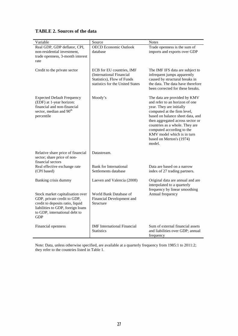
TABLE 2. Sources of the data Variable Source Notes Real GDP, GDP deflator, CPI, non-residential investment, trade openness, 3-month interest rate

OECD Economic Outlook database

Trade openness is the sum of imports and exports over GDP

Credit to the private sector ECB for EU countries, IMF (International Financial Statistics), Flow of Funds statistics for the United States

The IMF IFS data are subject to infrequent jumps apparently caused by structural breaks in the data. The data have therefore been corrected for these breaks.

Expected Default Frequency (EDF) at 1-year horizon: financial and non-financial sector, median and 90th percentile

Moody’s The data are provided by KMV and refer to an horizon of one year. They are initially computed at the firm level, based on balance sheet data, and then aggregated across sector or countries as a whole. They are computed according to the KMV model which is in turn based on Merton's (1974) model.

Relative share price of financial sector; share price of non-financial sectors

Datastream.

Real effective exchange rate (CPI based)

Bank for International Settlements database

Data are based on a narrow index of 27 trading partners.

Banking crisis dummy Laeven and Valencia (2008) Original data are annual and are interpolated to a quarterly frequency by linear smoothing

Stock market capitalisation over GDP, private credit to GDP, credit to deposits ratio, liquid liabilities to GDP, foreign loans to GDP, international debt to GDP

World Bank Database of Financial Development and Structure

Annual frequency

Financial openness IMF International Financial Statistics

Sum of external financial assets and liabilities over GDP; annual frequency

Note: Data, unless otherwise specified, are available at a quarterly frequency from 1985:1 to 2011:2; they refer to the countries listed in Table 1.

27

TABLE 3. Summary statistics

Variable Obs Mean Std. Dev. Min MaxLog CPI 2174 0.00 1.00 -2.89 1.66

Log real GDP 2248 0.00 1.00 -2.67 1.85Log investment 2248 0.00 1.00 -2.85 1.94Short term rate 2244 5.72 4.09 0.03 25.78

Log relative share price of fin. sector 2162 0.00 0.66 -3.63 5.01Credit growth 2172 0.03 0.04 -0.34 0.34

Log real effective exch. rate 2246 4.59 0.10 4.24 5.05EDF fin. Sector 1349 0.37 0.69 0.01 8.48

EDF non-fin. Sector 1274 0.55 0.50 0.02 3.23EDF fin. Sector, 90th percentile 1349 3.98 5.17 0.06 35.00

EDF non.fin sector, 90th percentile 1274 7.56 7.24 0.15 35.00Output gap 2248 0.00 0.08 -0.49 0.34

Real GDP growth 2227 0.03 0.05 -0.40 0.33Banking crisis dummy 2268 0.17 0.37 0.00 1.00

Note: The sample period is 1980:1 to 2011:2 (or longest available period), quarterly data. See Table 2 for the sources of the data. Note that data for the CPI have been seasonally adjusted using the X12 ARIMA approach. For the country list and the sources of the data see Tables 1-2.

28

TABLE 4. Panel regression, log relative share price of financial sector vs. non-financial sector (1) (2) (3) (4) (5) (6) Log relative share price of fin. sector, t-1 0.9135*** 0.9137*** 0.9134*** 0.9311*** 0.9400*** 0.9355*** (0.0188) (0.0190) (0.0189) (0.0190) (0.0162) (0.0194) Output gap 0.0282 0.0213 -0.0458 -0.0320 -0.0745 (0.0825) (0.0790) (0.0762) (0.0988) (0.0963) Real GDP growth 0.0267 (0.2422) Banking crisis dummy -0.0781** -0.1185** (0.0314) (0.0436) EDF of financial sector -0.0195 -0.0291** (0.0198) (0.0120) EDF of non-financial sector -0.0292 -0.0040 (0.0182) (0.0173) Observations 2,122 2,121 2,122 1,347 1,272 1,272 Number of countries 21 21 21 18 17 17 R2 Within 0.869 0.869 0.869 0.903 0.915 0.916 R2 Between 0.658 0.667 0.632 0.974 0.971 0.972 R2 Overall 0.868 0.868 0.869 0.904 0.916 0.917 Adj. R2 0.862 0.862 0.862 0.897 0.909 0.910

Note: Pooled OLS. The sample period is 1985:1 to 2011:2. The model includes country fixed effects and time dummies. Robust standard errors in parentheses, */**/*** denotes significance at the 10%/5%/1% level. The output gap is obtained by applying the HP1600 filter to the log of real GDP. See Table 2 on the sources and definitions of the variables.

29

TABLE 5. Variance decomposition of selected shocks

Non-financial demand shock Monetary policy shock Financial shock Other shocksCPI 18.8 14.8 9.5 56.8

Real GDP 14.7 19.1 11.8 54.3Investment 10.8 15.7 10.9 62.6

Short term rate 16.3 18.9 14.0 50.7Relative share price of fin. sector 11.7 10.4 16.5 61.4

Credit to the private sector 14.7 16.7 16.4 52.2Share price of non-fin. sector 13.0 11.7 14.8 60.6

Note: the table shows the variance decomposition at 24 quarters horizon. This is based on VAR models estimated on each country separately, and aggregated using the stochastic pooling approach (see Annex in the text). The variance decomposition is based on a single model per country, which ensures that the structural shocks are orthogonal among each other. The sample period is 1985:1 to 2011:2.

30

TABLE 6. Average cross-section correlation among estimated structural shocks

Average corr. Average absolute corr.Non-fin. demand shock 0.04 0.12

Mon. pol. shock 0.06 0.14Financial shock 0.07 0.15

Note: The table reports the average correlation among the estimated structural shocks, identified using the sign restrictions approach. See the notes to Figure 5 for additional information. The sample period is 1985:1 to 2011:2. TABLE 7. Structural indicators

Low countries High countriesPrivate credit / GDP 0.73 11 1.15 10Financial openness 1.39 11 5.45 10

Foreign loans / GDP 0.19 11 0.72 10International debt / GDP 0.20 11 0.41 10Liquid liabilities / GDP 0.56 11 0.95 10

Trade openness 0.48 11 0.95 10Stock mkt. cap. / GDP 0.41 10 1.00 10

Note: The table reports sample averages of the chosen structural indicators. ‘Low’ is the average of the countries which are below the median, and ‘High’ the number of countries which are above the median. The median values are computed on the longest available sample for each country. Computing averages over the longest joint sample leads to very similar results.

31

FIGURE 1. Relative share price of the financial sector vs. non-financial sector in the United States, in logs

-1.6

-1.2

-0.8

-0.4

0.0

0.4

0.8

1980 1985 1990 1995 2000 2005 2010

Note: Sectoral stock price data are from Datastream. See Table 2 for the sources of the data. FIGURE 2. Relative share price of the financial sector vs. non-financial sector in Ireland and Finland, in logs

-4

-3

-2

-1

0

1

2

1980 1985 1990 1995 2000 2005 2010

Finland Ireland

Note: Sectoral stock price data are from Datastream. See Table 2 for the sources of the data.

32

FIGURE 3. Log relative share price of the financial sector (blue line) and log relative share price of the high-leverage firms vs. low-leverage firms (red line)

-1.5

-1.0

-0.5

0.0

0.5

1.0

-.05

.00

.05

.10

.15

.20

1980 1985 1990 1995 2000 2005 2010

Log relative share price of high-levered firms vs low-levered firmsLog relative share of financial vs. non-financial sector

Note: The relative share price of the financial sector is reported on the right axis, the relative share price of high-leverage firms on the left axis.

33

FIGURE 4. Impulse responses to structural shocks

-.002.000.002.004.006.008.010

5 10 15 20

CPI

.00

.01

.02

.03

.04

.05

.06

.07

5 10 15 20

CPI

-.0004

-.0003

-.0002

-.0001

.0000

.0001

5 10 15 20

CPI

-.0050-.0025.0000.0025.0050.0075.0100.0125

5 10 15 20

Real GDP

-.04.00.04.08.12.16.20

5 10 15 20

Real GDP

-.0002

.0000

.0002

.0004

.0006

.0008

5 10 15 20

Real GDP

-.01

.00

.01

.02

.03

.04

5 10 15 20

Investment

-.1.0.1.2.3.4.5.6

5 10 15 20

Investment

-.001.000.001.002.003.004.005

5 10 15 20

Investment

-.05.00.05.10.15.20.25

5 10 15 20

Short term interest rate

-1.2

-0.8

-0.4

0.0

0.4

5 10 15 20

Short term interest rate

-.004

.004

.012

.020

.028

5 10 15 20

Short term interest rate

-.10-.08-.06-.04-.02.00.02.04

5 10 15 20

Relative share price of fin. sector

-.4

-.3

-.2

-.1

.0

.1

5 10 15 20

Relative share price of fin. sector

-.002

.002

.006

.010

.014

5 10 15 20

Relative share price of fin. sector

-.004

-.002

.000

.002

.004

.006

5 10 15 20

Credit to the private sector

-.04-.02.00.02.04.06.08

5 10 15 20

Credit to the private sector

-.0004

.0000

.0004

.0008

.0012

.0016

5 10 15 20

Credit to the private sector

-.03-.02-.01.00.01.02.03

5 10 15 20

Share price of non-fin. sector

-.1

.1

.3

.5

.7

5 10 15 20

Share price of non-fin. sector

-.002-.001.000.001.002.003.004.005

5 10 15 20

Share price of non-fin. sector

Non fin. demand shock Mon. pol. shock Financial shock

Note: The chart reports impulse responses to structural shocks identified by applying sign restrictions as in Rubio-Ramirez, Waggoner and Zha (2010). The size of the shocks is 100 basis points of the interest rate for the monetary policy shock; a rise by 1% of the standardised level of real GDP for the demand shock; and a rise of 1% of the standardised level of the relative share price of the financial sector for the financial shock. The impulse responses are based on a VAR model estimated on quarterly data from 1985:1 to 2011:2 on 21 countries, and after aggregating cross country impulse responses by applying the stochastic pooling approach (see text and Annex for further explanation).

34

FIGURE 5. Impulse responses to structural shocks, stochastic pooling (thin blue lines) vs. simple average (thick red line)

-.002.000.002.004.006.008.010

5 10 15 20

CPI

.00

.02

.04

.06

.08

.10

.12

5 10 15 20

CPI

-.0006-.0004-.0002.0000.0002.0004.0006

5 10 15 20

CPI

-.008-.004.000.004.008.012.016

5 10 15 20

Real GDP

-.04.00.04.08.12.16.20

5 10 15 20

Real GDP

-.0004-.0002.0000.0002.0004.0006.0008

5 10 15 20

Real GDP

-.010

.000

.010

.020

.030

5 10 15 20

Investment

-.1.0.1.2.3.4.5.6

5 10 15 20

Investment

-.002

.000

.002

.004

.006

5 10 15 20

Investment

-.05.00.05.10.15.20.25

5 10 15 20

Short term interest rate

-1.2-0.8-0.40.00.40.81.2

5 10 15 20

Short term interest rate

-.01

.00

.01

.02

.03

5 10 15 20

Short term interest rate

-.10-.08-.06-.04-.02.00.02.04

5 10 15 20

Relative share price of fin. sector

-.6-.5-.4-.3-.2-.1.0.1

5 10 15 20

Relative share price of fin. sector

-.002

.002

.006

.010

.014

5 10 15 20

Relative share price of fin. sector

-.008-.006-.004-.002.000.002.004.006

5 10 15 20

Credit to the private sector

-.02.00.02.04.06.08.10

5 10 15 20

Credit to the private sector

-.0008-.0004.0000.0004.0008.0012.0016

5 10 15 20

Credit to the private sector

-.03-.02-.01.00.01.02.03

5 10 15 20

Share price of non-fin. sector

-0.20.00.20.40.60.81.0

5 10 15 20

Share price of non-fin. sector

-.002

.000

.002

.004

.006

5 10 15 20

Share price of non-fin. sector

Non fin. demand shock Mon. pol. shock Financial shock

Note: Thin, blue lines are impulse responses to structural shocks identified by applying sign restrictions as in Rubio-Ramirez, Waggoner and Zha (2010) and aggregated across countries using the stochastic pooling approach. The size of the shocks is 100 basis points of the interest rate for the monetary policy shock; a rise by 1% of the standardised level of real GDP for the demand shock; and a rise of 1% of the standardised level of the relative share price of the financial sector for the financial shock. The impulse responses are based on a VAR model estimated on quarterly data from 1985:1 to 2011:2 on 21 countries, and after aggregating cross country impulse responses by applying the stochastic pooling approach (see text and Annex for further explanation). The thick red lines report the same impulse responses which are aggregated across countries by taking the arithmetic average across them without any further adjustment, and assuming that countries are independent among each other.

35

FIGURE 6. Impulse responses to structural shocks, full sample (thin blue lines) vs. excluding the 2007-09 global financial crisis (thick red line)

-.002.000.002.004.006.008.010.012

5 10 15 20

CPI

.00

.02

.04

.06

.08

5 10 15 20

CPI

-.0004-.0003-.0002-.0001.0000.0001.0002

5 10 15 20

CPI

-.0050-.0025.0000.0025.0050.0075.0100.0125

5 10 15 20

Real GDP

-.04.00.04.08.12.16.20

5 10 15 20

Real GDP

-.0004-.0002.0000.0002.0004.0006.0008.0010

5 10 15 20

Real GDP

-.01

.00

.01

.02

.03

.04

5 10 15 20

Investment

-.1.0.1.2.3.4.5.6

5 10 15 20

Investment

-.001

.001

.003

.005

.007

5 10 15 20

Investment

-.05.00.05.10.15.20.25.30

5 10 15 20

Short term interest rate

-1.2

-0.8

-0.4

0.0

0.4

5 10 15 20

Short term interest rate

-.01

.00

.01

.02

.03

.04

5 10 15 20

Short term interest rate

-.10-.08-.06-.04-.02.00.02.04

5 10 15 20

Relative share price of fin. sector

-.4-.3-.2-.1.0.1.2

5 10 15 20

Relative share price of fin. sector

-.004

.000

.004

.008

.012

.016

5 10 15 20

Relative share price of fin. sector

-.010

-.006

-.002

.002

.006

5 10 15 20

Credit to the private sector

-.04-.02.00.02.04.06.08

5 10 15 20

Credit to the private sector

-.0004.0000.0004.0008.0012.0016.0020

5 10 15 20

Credit to the private sector

-.04-.03-.02-.01.00.01.02.03

5 10 15 20

Share price of non-fin. sector

-.1

.1

.3

.5

.7

5 10 15 20

Share price of non-fin. sector

-.004

-.002

.000

.002

.004

.006

5 10 15 20

Share price of non-fin. sector

Non fin. demand shock Mon. pol. shock Financial shock

Note: Thin, blue lines are impulse responses to structural shocks identified by applying sign restrictions as in Rubio-Ramirez, Waggoner and Zha (2010) and aggregated across countries using the stochastic pooling approach. The size of the shocks is 100 basis points of the interest rate for the monetary policy shock; a rise by 1% of the standardised level of real GDP for the demand shock; and a rise of 1% of the standardised level of the relative share price of the financial sector for the financial shock. The impulse responses are based on a VAR model estimated on quarterly data from 1985:1 to 2011:2 on 21 countries, and after aggregating cross country impulse responses by applying the stochastic pooling approach (see text and Annex for further explanation). The thick red lines report the same impulse responses when the VAR models are estimated up to 2007:2.

36

FIGURE 7. Impulse responses to structural shocks, basedline vs. excluding euro area countries from 1999 (baseline in thin blue lines, excluding euro area countries in thick red lines)

-.002.000.002.004.006.008.010.012

5 10 15 20

CPI

-.2-.1.0.1.2.3.4.5

5 10 15 20

CPI

-.0006

-.0004

-.0002

.0000

.0002

5 10 15 20

CPI

-.0050-.0025.0000.0025.0050.0075.0100.0125

5 10 15 20

Real GDP

-0.20.00.20.40.60.81.0

5 10 15 20

Real GDP

-.0002.0000.0002.0004.0006.0008.0010

5 10 15 20

Real GDP

-.010

.000

.010

.020

.030

5 10 15 20

Investment

-0.5

0.0

0.5

1.0

1.5

2.0

5 10 15 20

Investment

-.001

.001

.003

.005

.007

5 10 15 20

Investment

-.08

.00

.08

.16

.24

5 10 15 20

Short term interest rate

-1.2

-0.8

-0.4

0.0

0.4

0.8

5 10 15 20

Short term interest rate

-.01

.00

.01

.02

.03

.04

5 10 15 20

Short term interest rate

-.10-.08-.06-.04-.02.00.02.04

5 10 15 20

Relative share price of fin. sector

-6-4-20246

5 10 15 20

Relative share price of fin. sector

-.0050-.0025.0000.0025.0050.0075.0100.0125

5 10 15 20

Relative share price of fin. sector

-.006-.004-.002.000.002.004.006

5 10 15 20

Credit to the private sector

-.6-.4-.2.0.2.4.6.8

5 10 15 20

Credit to the private sector

-.0004.0000.0004.0008.0012.0016.0020

5 10 15 20

Credit to the private sector

-.03-.02-.01.00.01.02.03

5 10 15 20

Share price of non-fin. sector

-0.5

0.0

0.5

1.0

1.5

2.0

5 10 15 20

Share price of non-fin. sector

-.002

.000

.002

.004

.006

5 10 15 20

Share price of non-fin. sector

Non fin. demand shock Mon. pol. shock Financial shock

Note: Thin, blue lines are impulse responses to structural shocks identified by applying sign restrictions as in Rubio-Ramirez, Waggoner and Zha (2010) and aggregated across countries using the stochastic pooling approach. The size of the shocks is 100 basis points of the interest rate for the monetary policy shock; a rise by 1% of the standardised level of real GDP for the demand shock; and a rise of 1% of the standardised level of the relative share price of the financial sector for the financial shock. The impulse responses are based on a VAR model estimated on quarterly data from 1985:1 to 2011:2 on 21 countries, and after aggregating cross country impulse responses by applying the stochastic pooling approach (see text and Annex for further explanation). The thick red lines report the same impulse responses when the VAR models are estimated after excluding observations for euro area countries after 1999..

37

FIGURE 8. Impulse responses to structural shocks, including foreign variables in the VAR, depending on countries’ private credit to GDP ratio (‘high’ countries in thick red lines, ‘low’ countries in thin blue)

-0.8

-0.4

0.0

0.4

0.8

1.2

5 10 15 20

CPI

-.02

.00

.02

.04

.06

.08

.10

5 10 15 20

CPI

-.05-.04-.03-.02-.01.00.01.02.03

5 10 15 20

CPI

-0.8

-0.4

0.0

0.4

0.8

1.2

1.6

5 10 15 20

Real GDP

-.05

.00

.05

.10

.15

.20

.25

5 10 15 20

Real GDP

-.06-.04-.02.00.02.04.06.08

5 10 15 20

Real GDP

-2

-1

0

1

2

3

4

5 10 15 20

Investment

-.2

.0

.2

.4

.6

.8

5 10 15 20

Investment

-.2

.0

.2

.4

.6

.8

5 10 15 20

Investment

-10-505

1015202530

5 10 15 20

Short term interest rate

-1.6

-1.2

-0.8

-0.4

0.0

0.4

0.8

5 10 15 20

Short term interest rate

-1

0

1

2

3

4

5 10 15 20

Short term interest rate

-12-10-8-6-4-2024

5 10 15 20

Relative share price of fin. sector

-.6

-.4

-.2

.0

.2

.4

5 10 15 20

Relative share price of fin. sector

-0.4

0.0

0.4

0.8

1.2

1.6

5 10 15 20

Relative share price of fin. sector

-1.5

-1.0

-0.5

0.0

0.5

1.0

1.5

5 10 15 20

Credit to the private sector

-.08

-.04

.00

.04

.08

.12

5 10 15 20

Credit to the private sector

-.04

.00

.04

.08

.12

.16

.20

5 10 15 20

Credit to the private sector

-4-3-2-101234

5 10 15 20

Share price of non-fin. sector

-0.2

0.0

0.2

0.4

0.6

0.8

1.0

5 10 15 20

Share price of non-fin. sector

-.4

-.2

.0

.2

.4

.6

5 10 15 20

Share price of non-fin. sector

Demand shock Monetary policy shock Financial shock

Note: See notes to Figure 5 on how impulse responses are computed. In this Figure, we divide countries in two groups according to whether they are above or below the median in terms of private credit to GDP ratio. Within each sub-group, countries are aggregated using the stochastic pooling approach. Impulse responses are shown in thin, blue lines for countries with a low reading of this structural indicator, and thick red lines for high readings.

38

FIGURE 9. Impulse responses to structural shocks, including foreign variables in the VAR, depending on countries’ financial openness (‘high’ countries in thick red lines, ‘low’ countries in thin blue)

-0.4-0.20.00.20.40.60.81.01.2

5 10 15 20

CPI

.00

.02

.04

.06

.08

.10

.12

5 10 15 20

CPI

-.08-.06-.04-.02.00.02.04.06

5 10 15 20

CPI

-0.8

-0.4

0.0

0.4

0.8

1.2

1.6

5 10 15 20

Real GDP

-.05

.00

.05

.10

.15

.20

5 10 15 20

Real GDP

-.06-.04-.02.00.02.04.06.08.10

5 10 15 20

Real GDP

-2

-1

0

1

2

3

4

5 10 15 20

Investment

-.2

.0

.2

.4

.6

.8

5 10 15 20

Investment

-.2

.0

.2

.4

.6

.8

5 10 15 20

Investment

-8-4048

1216202428

5 10 15 20

Short term interest rate

-1.6

-1.2

-0.8

-0.4

0.0

0.4

0.8

5 10 15 20

Short term interest rate

-1

0

1

2

3

4

5 10 15 20

Short term interest rate

-10-8-6-4-2024

5 10 15 20

Relative share price of fin. sector

-.6

-.4

-.2

.0

.2

.4

.6

5 10 15 20

Relative share price of fin. sector

-0.5

0.0

0.5

1.0

1.5

5 10 15 20

Relative share price of fin. sector

-0.8

-0.4

0.0

0.4

0.8

1.2

5 10 15 20

Credit to the private sector

-.12

-.08

-.04

.00

.04

.08

.12

5 10 15 20

Credit to the private sector

-.04

.00

.04

.08

.12

.16

5 10 15 20

Credit to the private sector

-6

-4

-2

0

2

4

6

5 10 15 20

Share price of non-fin. sector

-0.2

0.0

0.2

0.4

0.6

0.8

1.0

5 10 15 20

Share price of non-fin. sector

-.4

-.2

.0

.2

.4

.6

.8

5 10 15 20

Share price of non-fin. sector

Demand shock Monetary policy shock Financial shock

Note: See notes to Figure 5 on how impulse responses are computed. In this Figure, we divide countries in two groups according to whether they are above or below the median in terms of financial openness (sum of cross border financial assets and liabilities over GDP). Within each sub-group, countries are aggregated using the stochastic pooling approach. Impulse responses are shown in thin, blue lines for countries with a low reading of this structural indicator, and thick red lines for high readings.

39

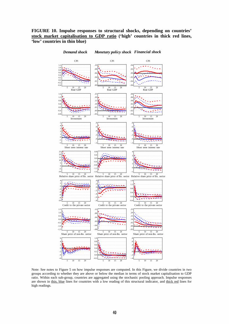
FIGURE 10. Impulse responses to structural shocks, depending on countries’ stock market capitalisation to GDP ratio (‘high’ countries in thick red lines, ‘low’ countries in thin blue)

-0.4-0.20.00.20.40.60.81.01.2

5 10 15 20

CPI

.00

.02

.04

.06

.08

.10

5 10 15 20

CPI

-.06

-.04

-.02

.00

.02

.04

5 10 15 20

CPI

-0.8

-0.4

0.0

0.4

0.8

1.2

1.6

5 10 15 20

Real GDP

-.05

.00

.05

.10

.15

.20

.25

5 10 15 20

Real GDP

-.04

-.02

.00

.02

.04

.06

.08

5 10 15 20

Real GDP

-2-1012345

5 10 15 20

Investment

-.2

.0

.2

.4

.6

.8

5 10 15 20

Investment

-.2

.0

.2

.4

.6

.8

5 10 15 20

Investment

-10-505

10152025

5 10 15 20

Short term interest rate

-1.6

-1.2

-0.8

-0.4

0.0

0.4

0.8

5 10 15 20

Short term interest rate

-1

0

1

2

3

4

5 10 15 20

Short term interest rate

-10-8-6-4-2024

5 10 15 20

Relative share price of fin. sector

-.8

-.6

-.4

-.2

.0

.2

.4

5 10 15 20

Relative share price of fin. sector

-0.4

0.0

0.4

0.8

1.2

1.6

5 10 15 20

Relative share price of fin. sector

-1.5

-1.0

-0.5

0.0

0.5

1.0

1.5

5 10 15 20

Credit to the private sector

-.08

-.04

.00

.04

.08

.12

5 10 15 20

Credit to the private sector

-.05

.00

.05

.10

.15

.20

.25

5 10 15 20

Credit to the private sector

-6

-4

-2

0

2

4

6

5 10 15 20

Share price of non-fin. sector

-0.2

0.0

0.2

0.4

0.6

0.8

1.0

5 10 15 20

Share price of non-fin. sector

-.4

-.2

.0

.2

.4

.6

.8

5 10 15 20

Share price of non-fin. sector

Demand shock Monetary policy shock Financial shock

Note: See notes to Figure 5 on how impulse responses are computed. In this Figure, we divide countries in two groups according to whether they are above or below the median in terms of stock market capitalisation to GDP ratio. Within each sub-group, countries are aggregated using the stochastic pooling approach. Impulse responses are shown in thin, blue lines for countries with a low reading of this structural indicator, and thick red lines for high readings.

40