FEDERAL RESERVE BANK OF SAN FRANCISCO

WORKING PAPER SERIES

Working Paper 2009-05 http://www.frbsf.org/publications/economics/papers/2009/wp09-05bk.pdf

The views in this paper are solely the responsibility of the authors and should not be interpreted as reflecting the views of the Federal Reserve Bank of San Francisco or the Board of Governors of the Federal Reserve System.

What do we know and not know about potential output?

Susanto Basu Boston College and NBER

John G. Fernald

FRB San Francisco

March 2009

Preliminary Comments welcome

What do we know and not know about potential output?

by

Susanto Basu and John G. Fernald*

First draft: October 11, 2008 This draft: March 9, 2009

Abstract: Potential output is an important concept in economics. Policymakers often use

a one-sector neoclassical model to think about long-run growth, and often assume that potential output is a smooth series in the short-run—approximated by a medium- or long-run estimate. But in both the short- and long-run, the one-sector model falls short empirically, reflecting the importance of rapid technical change in producing investment goods; and few, if any, modern macroeconomic models would imply that, at business cycle frequencies, potential output is a smooth series. Discussing these points allows us to discuss a range of other issues that are less well understood, and where further research could be valuable.

*Boston College and NBER, susanto.basu@bc.edu; and Federal Reserve Bank of San Francisco, John.Fernald@sf.frb.org. We thank Alessandro Barattieri and Kyle Matoba for outstanding research assistance, and Jonas Fisher and Miles Kimball for helpful discussions and collaboration on related research. We also thank Bart Hobijn, Chad Jones, John Williams, Rody Manuelli, and conference participants for helpful discussions and comments. The views expressed are those of the authors, and do not necessarily reflect the views of anyone else affiliated with the Federal Reserve System.

2

Introduction

The concept of potential output plays a central role in policy discussions. In the long run,

faster growth in potential output leads to faster growth in actual output and, for given trends in

population and workforce, faster growth in incomes per capita. In the short run, policymakers

need to assess the degree to which fluctuations in observed output reflect the optimal response to

shocks that hit the economy, versus undesirable fluctuations.

To keep the discussion manageable, we confine our discussion of potential output to

neoclassical growth models with exogenous technical progress, in the short and the long run; we

also focus exclusively on the United States. We make two main points. First, in both the short

and the long run, the rapid pace of technological change in producing equipment investment

goods is important. This rapid technical change in investment goods implies that the two-sector

neoclassical model—where one sector produces investment goods and the other produces

consumption goods—provides a better benchmark for thinking about potential output than the

one-sector growth model. Second, in the short run, the measure of potential output that matters

for policymakers is likely to fluctuate substantially over time. Neither macroeconomic theory

nor existing empirical evidence suggest that potential output is a smooth series. Policymakers,

however, often appear to assume that, even in the short run, potential output is well

approximated by a smooth trend.1 Our model and empirical work corroborate these two points

and provide a framework to discuss other aspects of what we know, and do not know, about

potential output.

To begin, though, it’s important to be clear on definitions: “Potential output” is often

used to describe related, but logically distinct, concepts. First, people often mean something akin

to a forecast for output and its growth rate in the longer run (say, 10 years out). We will often 1 See, for example, CBO (2001, 2004) and OECD (2008).

3

refer to this first concept as a steady-state measure, although it might differ in models such as

Jones (2002), who interprets the past century as a time when growth in output per capita was

relatively constant at a rate above steady state; a decade-long forecast can also incorporate

transition dynamics towards steady state.

But in the short run, a steady-state notion is less relevant for policymakers who are

thinking about stabilizing output or inflation at high frequencies. This leads to a second concept,

explicit in New Keynesian models dynamic stochastic general equilibrium (DSGE) models:

potential output is the rate of output the economy would have if there were no nominal rigidities,

but all other (real) frictions and shocks were unchanged.2 In a flexible-price real-business-cycle

model, where prices adjust instantaneously, potential output is equivalent to actual, equilibrium

output. In contrast to the first long-term definition of potential output, the second, short-term

meaning is likely to fluctuate in the short run because shocks push the economy temporarily

away from steady state.

In New Keynesian models, where prices and/or wages might adjust slowly towards their

long-run equilibrium values, actual output might well deviate from this short-term measure of

potential output. In many of these models, the “output gap”—the difference between actual and

potential output—is the key variable in determining the evolution of inflation. Thus, this second

definition also corresponds to the older Keynesian notion that potential output is “the maximum

production without inflationary pressure” (Okun, 1970, pp132-22), i.e., the level of output at

which there is no pressure for inflation to either increase or decrease. In most if not all

macroeconomic models, the second (flexible price) definition converges in the long run to the

first, steady-state definition.

2 See Woodford (2003) for the theory. Neiss and Nelson (2005) construct an output gap from a small, one-

sector DSGE model.

4

Third, in an economy with frictions such as monopolistic competition, potential output

could be taken to be the current optimal rate of output. With market imperfections, neither

steady-state output, nor the flexible-price equilibrium level of output, needs to be optimal or

efficient. Like the first two concepts, this third meaning is of interest to policymakers who might

seek to improve the efficiency of the economy. (However, decades of research on time-

inconsistency suggests that such policies should be implemented by fiscal or regulatory

authorities, who can target the imperfections directly, but not by the central bank, which

typically must take these imperfections as given. See, for example, the seminal paper by

Kydland and Prescott, 1977.)3

The first part of our paper focuses on long-term growth, which is clearly of first-order

importance for the economy, especially in discussions of fiscal policy. For example, whether

promised entitlement spending is feasible depends almost entirely on long-run growth. We show

that the predictions of two-sector models lead us to be more optimistic about the economy’s

long-run growth potential. This part of our paper will thus be of interest to fiscal policy makers.

The second part of our paper focuses primarily on potential output for monetary policy

makers, where it is most natural to think about the current, flexible-price equilibrium level of

output—the second usage above. Potential output plays a central, if often implicit, role in

monetary policy decisions. The Federal Reserve has a dual mandate to pursue low and stable

inflation and maximum sustainable employment. Maximum sustainable employment is usually

interpreted to imply that the Federal Reserve should strive, subject to its other mandate, to

stabilize the real economy around its flexible-price equilibrium level, in order to avoid inefficient

3 Justiniano and Primiceri (2008) define “potential output” as this third measure, with no market

imperfections; they use the term “natural output” to mean our second, flexible wage/price measure.

5

and undesirable fluctuations in employment. In New Keynesian models, deviations of actual

from potential output put pressure on inflation.

Section I of this paper compares the steady-state implications of one- and two-sector

neoclassical models with exogenous technological progress. That is, we focus on for the long-

run effects of given trends in technology, rather than trying to understand the sources of this

technological progress.4 Understanding where technology comes from is central for

policymakers thinking about policies to promote long-run growth, but it is beyond the scope of

our paper. In Section II, we use the two-sector model to present a range of possible scenarios for

long-term productivity growth, and discuss some of the questions that arise in contemplating the

likelihood of the different scenarios.

In Section III, we turn to short-term implications, asking whether it is plausible to think

of potential output as being a smooth process, and comparing implications of a simple one-sector

versus two-sector model. Section IV turns to the current situation, as of late 2008: How does

short-run potential output growth compare with its steady-state level? This discussion suggests a

number of additional issues that are unknown, or difficult to quantify. Section V concludes.

I. The long run: What simple model matches the data?

A common, and fairly sensible, approach for estimating steady-state output growth is to

estimate growth in full-employment labor productivity and then allow for demographics to

determine the evolution of the labor force. This approach motivates a focus in this section on

assessing steady-state labor productivity growth.

4 Of course, TFP can change for reasons broader than technological change alone: improved institutions,

deregulation, and less distortionary taxes are only some of the reasons. We believe, however, that long-run trends in TFP in developed countries like the United States are driven primarily by technological change.

6

We generally think that, in the long run, different forces explain labor productivity and

total hours worked—technology along with induced capital deepening explains the former and

demographics explains the latter. The assumption that labor productivity evolves separately

from hours worked is motivated by the observation that labor productivity has risen dramatically

over the past two centuries, whereas household labor supply has changed by much less.5 Noting

the common U-shaped pattern in hours worked and labor productivity growth in the post-World-

War period in the United States, Elsby and Shapiro (2008) question this separation between labor

productivity and hours worked, on the grounds that incentives to invest in a career likely depends

on trend productivity. Jones (1995), in addition suggests an endogenous-growth mechanism for

linking technology and demographics. Despite these counterexamples to separability between

technology and demographics, the analysis that follows should capture key properties of the

endogenous response of capital deepening to technology change.

A reasonable way to arrive at an estimate of steady-state labor productivity growth is to

estimate underlying technology growth, and then use a model to calculate the implications for

capital deepening. Let hats over a variable represent log changes. As a matter of identities, we

can write output growth, y , as labor-productivity growth plus growth in hours worked, h :

ˆ ˆˆ ˆ( )y y h h= − + .

We focus here on full-employment labor productivity.

Suppose we define growth in total factor productivity, or the Solow residual, as

ˆ ˆˆ (1 )tfp y k lα α= − − − , where alpha is capital’s share of income and (1-α ) is labor’s share of

5 King, Plosser and Rebelo (1988) suggest that to a first approximation one should model hours per capita

as independent of the level of technology, and provide necessary and sufficient conditions on the utility function for this result to hold. Basu and Kimball (2002) show that the particular non-separability between consumption and work hours that is generally implied by the King-Plosser-Rebelo utility function helps explain the evolution of consumption in postwar U.S. data, and resolves several consumption puzzles.

7

income. Defining ˆ ˆl h lq≡ + , where lq is labor “quality” (composition) growth6, we can rewrite

output per hour growth as:

ˆ ˆ ˆˆ( ) ( )y h tfp k l lqα− = + − + . (1)

As an identity, growth in output per hour worked reflects TFP growth; the contribution of

capital deepening, defined as ˆ ˆ( )k lα − ;and increases in labor quality. Economic models suggest

mappings between fundamentals and the terms in this identity which are sometimes trivial, and

sometimes not.

A. The one-sector model

Perhaps the simplest model that could reasonably be applied to the long-run data is the

one-sector neoclassical growth model. Technological progress and labor force growth are

exogenous and capital deepening is endogenous.

We can derive the key implications from the textbook Solow version of the model.

Consider an aggregate production function 1( )Y K ALα α−= , where technology A grows at rate g,

and labor input L (which captures both raw hours H and labor quality LQ—henceforth, we do not

generally differentiate between the two) grows at rate n. Expressing all variables in terms of

“effective labor” AL yields:

y kα= , where /y Y AL= and /k K AL= . (2)

Capital accumulation takes place according to the perpetual-inventory formula. If s is the

saving rate, so that sy is investment per effective worker then, in steady-state: 6 Labor quality/composition reflects the mix of hours across workers with different levels of education,

experience, and so forth. For the purposes of this discussion, where we’re so far focused on definitions, suppose there were J types of workers with factor shares of income jβ , where (1 )jj

β α= −∑ . Then a reasonable

definition of TFP would be ˆ ˆˆ j jjtfp y k hα β= − −∑ . Growth accounting as done by the Bureau of Labor

Statistics or Jorgenson defines ˆ ˆ (1 )j jjl hβ α= −∑ , ˆ ln jj

h d H= ∑ , and ˆ ˆq l h= − .

8

( )sy n g kδ= + + (3)

Because of diminishing returns to capital, the economy converges to a steady state where

y and k are constant. At that point, investment per effective worker is just enough to offset the

effects of depreciation, population growth, and technological change on capital per effective

worker. In steady state, the unscaled levels of Y and K grow at rate g+n; capital-deepening, K/L,

grows at rate g. Labor productivity Y/L, i.e., output per unit of labor input, also grows at rate g.

From the production function, measured TFP growth is related to labor-augmenting

technology growth by:

ˆ ˆ ˆ(1 ) (1 )tfp Y K L gα α α= − − − = − .

The model maps directly to equation (1) above. In particular, the endogenous

contribution of capital deepening to labor-productivity growth is /(1 )g tfpα α α= ⋅ − . Output per

unit of labor input grows at rate g, which equals the sum of standard TFP growth (1 )gα− and

induced capital deepening gα .

Table 1, below, shows how this model performs relative to the data. It uses the

multifactor productivity release from the Bureau of Labor Statistics, which provides data for TFP

growth as well as capital deepening for the U.S. business economy. These are shown in the first

two columns. Note that, in the model above, standard TFP growth reflects technology alone. In

practice, a large literature suggests reasons why non-technological factors might affect measured

TFP growth. For example, there are hard-to-measure short-run movements in labor effort and

capital’s workweek, which move labor and total factor productivity around in the short-run.

Non-constant returns to scale and markups also interfere with the mapping from technology

change to measured aggregate total factor productivity. But the deviations between technology

and measured TFP are likely to be more important in the short run than in the long run,

9

consistent with the findings of Basu, Fernald, and Kimball (2006) and Basu, Fernald, Fisher, and

Kimball (2008). Hence, for these longer-term comparisons, we assume average TFP growth

reflects average technology growth.

Column 3 shows the predictions of the one-sector neoclassical model, for α = 0.32 (the

average value in the BLS multifactor dataset):

Table 1 One-sector growth model predictions for the U.S. Business Sector

Total TFP

Actual capital-

deepening contribution

Predicted capital-deepening

contribution in one-sector model

(1) (2) (3) 1948-2007 1.39 0.76 0.65

1948-1973 2.17 0.85 1.02 1973-1995 0.52 0.62 0.25 1995-2007 1.34 0.84 0.63 1995-2000 1.29 1.01 0.61 2000-2007 1.37 0.72 0.65

Note: Data for columns (1) and (2) are business-sector estimates from the BLS multifactor productivity database (downloaded via Haver on August 19, 2008). Capital and labor are adjusted for changes in composition. Actual capital deepening is ˆ ˆ( )k lα − , and predicted capital deepening is /(1 )tfpα α⋅ − .

Comparing columns (2) and (3), the model does not perform particularly well. It slightly

underestimates the contribution of capital deepening over the entire 1948-2007 period. But it

does a particularly poor job at matching the low-frequency variation in that contribution. In

particular, it somewhat overpredicts capital deepening for the pre-1973 period, but substantially

10

underpredicts for the 1973-95 period. That is, given the slowdown in TFP growth, the model

predicts a much larger slowdown in the contribution of capital deepening.7

One way to see the problem with the one-sector model graphically is to observe that the

model predicts a constant capital-output ratio in steady state—in contrast to the data. Figure 1

shows the sharp rise, since the mid-1960s, in the business-sector capital-output ratio:

Figure 1 Capital-output ratio in the United States (equipment and structures)

1

1.1

1.2

1.3

1.4

1.5

1.61.7

1

1950 1960 1970 1980 1990 2000

Index, 1947=1Ratio scale

Source: BLS multisector productivity database. Equipment and structures (i.e., fixed reproducible tangible capital capital) is calculated as a Tornquist index of the two categories. SIC data (from http://www.bls.gov/mfp/historicalsic.htm) is spliced to NAICS data (from http://www.bls.gov/mfp/mprdload.htm ) starting at 1988. (Data downloaded October 13, 2008.)

B. The two-sector model: A better match

7 Note that output per unit of quality-adjusted labor is the sum of TFP plus the capital deepening

contribution which, in the business sector, averaged 1.39+0.76=2.15 percent per year over the full sample. More commonly, labor productivity is reported as output per hour worked. Over the sample, labor quality in the BLS multifactor productivity dataset rose 0.36 percent per year, so output per hour rose 2.51 percent per year.

11

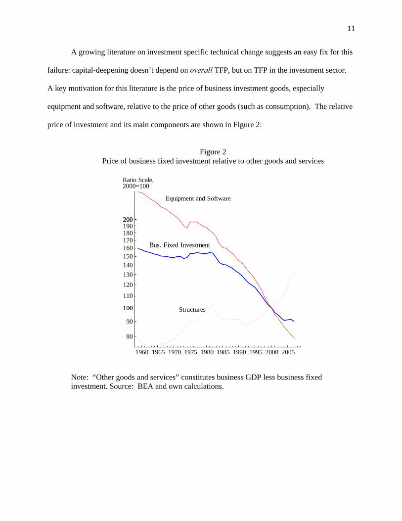
A growing literature on investment specific technical change suggests an easy fix for this

failure: capital-deepening doesn’t depend on overall TFP, but on TFP in the investment sector.

A key motivation for this literature is the price of business investment goods, especially

equipment and software, relative to the price of other goods (such as consumption). The relative

price of investment and its main components are shown in Figure 2:

Figure 2

Price of business fixed investment relative to other goods and services

Note: “Other goods and services” constitutes business GDP less business fixed investment. Source: BEA and own calculations.

80

90

100

110

120130140150160170180190200

100

200

1960 1965 1970 1975 1980 1985 1990 1995 2000 2005

Ratio Scale, 2000=100

Equipment and Software

Structures

Bus. Fixed Investment

12

Why do we see this steady relative price decline? The most natural interpretation is that

there is a more rapid pace of technical change in producing investment goods (especially high-

tech equipment).8

To see the implications of a two-sector model, consider a simple two-sector Solow-type

model, where s is the share of nominal output that is invested each period.9 One sector produces

investment goods that are used to create capital; the other sector produces consumption goods.

The two sectors use the same Cobb-Douglas production function, but with potentially different

technology levels:

1

1

( )

( )I I I

C I C

I K A L

C QK A L

α α

α α

−

−

=

=

In the consumption equation, we have implicitly defined labor-augmenting technological

change as 1/(1 )C IA Q Aα−= in order to decompose consumption technology into the product of

investment technology AI and a “consumption specific” piece, 1/(1 )Q α− . Let investment

technology AI grow at rate gI and the consumption-specific piece Q grow at rate q. Perfect

competition and cost-minimization imply that price equals marginal cost. If the sectors face the

same factor prices (and the same rate of indirect business taxes), then:

C

II

C

P MC QP MC

= =

The sectors also choose to produce with the same capital-labor ratios, implying that

I I I C I C IK A L K A L K A L= = . We can then write the production functions as:

8 On the growth accounting side, see, for example, Jorgenson (2001) or Oliner and Sichel (2000); see also

Greenwood, Hercowitz, and Krusell (1997). 9 This model is a fixed-saving rate version of the two-sector neoclassical growth model in Whelan (2000)

and is isomorphic to the one in Greenwood, Hercowitz, and Krusell (1997). Greenwood et al. choose a different normalization of the two technology shocks in their model.

13

( )( )

I I I

I C I

I A L K A L

C QA L K A L

α

α

=

=

We can now write the economy’s budget constraint in a simple manner:

( )Inv. Units [ / ] ( )I I C IY I C Q A L L K A L α≡ + = + , or

Inv. Unitsy kα= , where Inv. Units Inv. Units / Iy Y A L= and / Ik K A L= . (4)

Output here is expressed in investment units, and “effective labor” is in terms of

technology in the investment sector. The economy mechanically invests a share s of nominal

investment, which implies that investment per effective unit of labor is Inv. Unitsi s y= ⋅ .10 Capital

accumulation then takes the same form as in the one-sector model, except that it is only growth

in investment technology, gI, that matters. In particular, in steady state:

Inv. Units ( )Isy n g kδ= + + (5)

The production function (4) and capital-accumulation equation (5) correspond exactly to

their one-sector counterparts. Hence, the dynamics of capital in this model reflect technology in

the investment sector alone. In steady state, capital per unit of labor, K/L, grows at rate gI, so the

contribution of capital deepening to labor-productivity growth from equation (1) is

/(1 )I Ig tfpα α α= ⋅ − . Consumption technology in this model is “neutral,” in that it does not

affect investment or capital accumulation; the same result carries over to the Ramsey version of

this model, with or without variable labor supply. (Basu, Fernald, Fisher, and Kimball, 2008,

discuss the idea of consumption-technology neutrality in greater detail.) 11

10 [ ] ( )Inv. Units ( ) / /I I C C I I Is y P I P I P C I P C P A L I A L⋅ = + ⎡ + ⎤ =⎣ ⎦ 11 Note also that output in investment units is not equal to chain output in the national accounts. Chain

GDP is ˆˆ ˆ (1 )Y sI s C= + − . In contrast, in this model Inv. Units ˆˆ (1 ) (1 )Y sI s C s q= + − − − . Hence, Inv. Unitsˆ (1 )Y Y s q= + − .

14

To take this model to the data, we need to decompose aggregate TFP growth (calculated

from chained output) into its consumption and investment components. Given the conditions so

far, the following two equations hold:

(1 )I C

C I C I

tfp s tfp s tfp

P P tfp tfp

= ⋅ + −

− = −

These are two equations in two unknowns— Itfp and Ctfp . Hence, they allow us to

decompose aggregate TFP growth into investment and consumption TFP growth.12

Table 2 shows that the two-sector growth model does, in fact, fit the data rather better.

All derivations are done assuming an investment share of 0.15, about equal to the nominal value

of business fixed investment relative to the value of business output:

12 The calculations below use the official price deflators from the national accounts. Gordon (1990) argues

that many equipment deflators are not sufficiently adjusted for quality improvements over time. Much of the macroeconomic literature since then has used the Gordon deflators (possibly extrapolated, as in Cummins and Violante, 2002). Of course, as Whelan (2003) points out, much of the discussion of biases in the CPI involve service prices, which also miss a lot of quality improvements, making the overall effect .

15

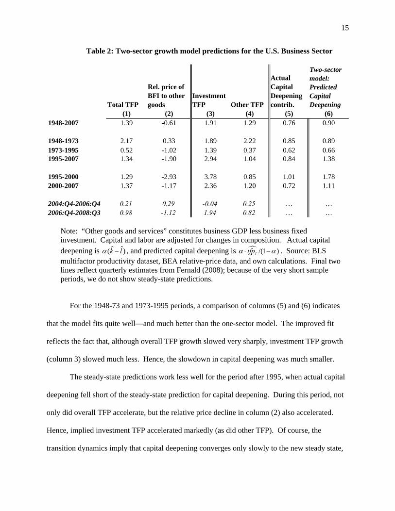
Table 2: Two-sector growth model predictions for the U.S. Business Sector

Total TFP

Rel. price of BFI to other goods

Investment TFP Other TFP

Actual Capital Deepening contrib.

Two-sector model: Predicted Capital Deepening

(1) (2) (3) (4) (5) (6)1948-2007 1.39 -0.61 1.91 1.29 0.76 0.90

1948-1973 2.17 0.33 1.89 2.22 0.85 0.891973-1995 0.52 -1.02 1.39 0.37 0.62 0.661995-2007 1.34 -1.90 2.94 1.04 0.84 1.38

1995-2000 1.29 -2.93 3.78 0.85 1.01 1.782000-2007 1.37 -1.17 2.36 1.20 0.72 1.11

2004:Q4-2006:Q4 0.21 0.29 -0.04 0.25 … …2006:Q4-2008:Q3 0.98 -1.12 1.94 0.82 … …

Note: “Other goods and services” constitutes business GDP less business fixed investment. Capital and labor are adjusted for changes in composition. Actual capital deepening is ˆ ˆ( )k lα − , and predicted capital deepening is /(1 )Itfpα α⋅ − . Source: BLS multifactor productivity dataset, BEA relative-price data, and own calculations. Final two lines reflect quarterly estimates from Fernald (2008); because of the very short sample periods, we do not show steady-state predictions.

For the 1948-73 and 1973-1995 periods, a comparison of columns (5) and (6) indicates

that the model fits quite well—and much better than the one-sector model. The improved fit

reflects the fact that, although overall TFP growth slowed very sharply, investment TFP growth

(column 3) slowed much less. Hence, the slowdown in capital deepening was much smaller.

The steady-state predictions work less well for the period after 1995, when actual capital

deepening fell short of the steady-state prediction for capital deepening. During this period, not

only did overall TFP accelerate, but the relative price decline in column (2) also accelerated.

Hence, implied investment TFP accelerated markedly (as did other TFP). Of course, the

transition dynamics imply that capital deepening converges only slowly to the new steady state,

16

and a decade is a relatively short period of time. (In addition, the pace of investment-sector TFP

was particularly rapid in the late 1990s, and has slowed somewhat in the 2000s.) So the more

important point is that qualitatively, the model works in the right direction even over this

relatively short period.

Despite these uncertainties, a bottom-line comparison of the one- and two-sector models

is of interest. Suppose that the 1995-2007 rates of TFP growth continue to hold, in both sectors

(a big “if” that we discuss in the next section). Suppose also that the two-sector model fits well

going forward, as it did in the 1948-95 period. Then we would project that in the future output

per hour (like output per quality-adjusted unit of labor, shown in Tables 1 and 2) will grow on

average about ¾ percentage point per year faster than the one-sector model would predict (1.38

versus 0.63), due to greater capital deepening. The difference is, clearly, substantial—e.g., it is a

significant fraction of the average 2.15 percent growth rate in output per unit of labor (and 2.5

percent growth rate of output per hour) over the 1948-2007 period.

II. Projecting the future

Forecasters, policymakers, and a number of academics regularly make “structured

guesses” about the likely path of future growth.13 Not surprisingly, the usual approach is to

assume that the future will look something like the past—but the challenge is to decide which

parts of the past to include, and which to downplay.

Viewed through the lens of the two-sector model, projections need to take a stand on TFP

growth in the investment sector, and TFP growth in the non-investment sector. We consider

three possibilities, labeled low, medium, and high, below.

13 Oliner and Sichel (2002) use the phrase “structured guesses.” In addition to Oliner and Sichel, recent

high-profile examples of projections have come from Jorgenson, Ho, and Stiroh (e.g., 2008) and Gordon (2006). The Congressional Budget Office and the Council of Economic Advisers regularly include longer-run projections of potential output.

17

Table 3 A range of estimates for steady-state labor productivity growth

Investment TFP Other TFP Overall TFP

Capital Deepening Contrib. Labor Prod.

Output per Hour worked

(1) (2) (3) (4) (5) (6)Low 1.00 0.70 0.7 0.5 1.2 1.5Med 2.00 0.85 1.0 0.9 2.0 2.3High 2.50 1.10 1.3 1.2 2.5 2.8

Notes: Calculations assume an investment share of output of 0.15 and a capital share in

production, α , of 0.32. Column (3) is an output-share-weighted average of columns (1) and (2). Column (4) is column (1) multiplied by (1 )α α− . Column (5) is output per unit of composition-adjusted labor input, and is the sum of columns (3) and (4). Column (6) adds an assumed growth rate of labor quality/composition of 0.3 percent per year, and therefore equals column (5) plus 0.3 percent.

Consider the medium scenario, which has output per hour growing at 2-1/4 percent

(column 6). Investment TFP is a bit slower than its average in the post-2000 period, reflecting

that investment TFP has been generally slowing since the burst of the late 1990s. Other TFP

slows to its rate in the second half of the 1990s, reflecting an assumption that the experience of

the early 2000s is unlikely to persist.

Productivity growth averaging 2-1/4 percent is comparable to estimates economists have

made recently. For example, in the first quarter of 2008, the median estimate in the Survey of

Professional Forecasters (SPF) was for 2 percent labor-productivity growth over the next 10

years (and 2-3/4 percent GDP growth).14 The Congressional Budget Office, in September, 2008,

estimated that labor productivity (in the non-farm business sector) would grow at an average rate

of about 2.2 percent between 2008 and 2018.15

14 http://www.philadelphiafed.org/research-and-data/real-time-center/survey-of-professional-

forecasters/2008/spfq108.pdf 15 Calculated from data in http://www.cbo.gov/ftpdocs/97xx/doc9706/Background_Table2-2.xls.

18

But as the table above makes clear, small and plausible changes in assumptions—well

within the range of recent experience—can make a large difference for steady-state growth

projections. As a result, there are a wide range of plausible outcomes. In the SPF, the standard

deviation across the 39 respondents for productivity growth over the next 10 years was about 0.4

percent—with a range of 0.9 to 3.0 percent. Indeed, the current median estimate of 2.0 percent is

down from an estimate of 2.5 percent in 2005; but remains much higher than the 1-year estimate

of only 1.3 percent in 1997.16

The two-sector model suggests several key questions in making long-run projections.

First, what will the pace of technical progress be in information technology (IT) and,

more broadly, in equipment? For example, for hardware, Moore’s Law and the semiconductor

replacement cycle (two versus three years) gives us plausible bounds. But for software, we

really have very little firm ground for speculation.

Second, how elastic is demand for IT? The discussion in Section I of the two-sector

model assumed that the share of investment was constant at 0.15. But an important part of the

price decline reflected the increasing share of IT, where prices have been falling rapidly, in total

BFI. At some point, a constant share is a reasonable assumption, and consistent with a balanced

growth path. But over the next few decades, one can imagine very different paths. Technology

optimists (such as DeLong, 2002) think that the elasticity of demand for IT exceeds unity, so that

demand will rise even faster than prices fall. They think that firms and individuals will find a

large number of new uses for computers, semiconductors, and, indeed, information, as these

commodities get cheaper and cheaper. By contrast, technology pessimists (such as Gordon,

2000) think that the greatest contribution of the IT revolution is in the past rather than the future.

16 The SPF has been asking about long-run projections in the first-quarter of each year since 1992. The

data are available http://www.philadelphiafed.org/research-and-data/real-time-center/survey-of-professional-forecasters/data-files/PROD10/ ..

19

For example, firms may decide they don’t need much more computing power in the future, so

that as prices continue to fall, the nominal share of expenditure on IT will also fall. For example,

for doing word processing, new and faster computers might offer few advantages relative to

existing computers, so the replacement cycle might become longer.

Third, what will happen to TFP in non-IT sectors? The range of uncertainty here is very

large—larger, arguably, than for the first two questions. The general-purpose-technology nature

of computing suggests that faster computers and better ability to manage and manipulate

information might well show up as TFP improvements in computer-using sectors.17 For

example, many important management innovations, such as the Walmart business model or the

widespread diffusion of warehouse automation, are made possible by cheap computing power.

Productivity in research and development may also rise more directly; auto parts manufacturers,

for example, can design new products on a computer rather than having to build physical models.

That is, computers may lower the cost and raise the returns to R&D.

Of course, one also needs to decide whether these sorts of TFP spillovers from IT to non-

IT sectors are best considered as growth effects or level effects. For example, the

‘Walmartization’ of retailing raises productivity levels (as more efficient producers expand and

less efficient producers contract) but does not necessarily boost long-run growth.

Fourth, the effects noted above might well depend on labor-market skills. Many

endogenous growth models incorporate a key role for human capital, which is surely a key input

into the innovation process—whether reflected in formal R&D or in management

17 See, for example, Basu, Fernald, Oulton, and Srinivasan (2003) for an interpretation of the broad-based

TFP acceleration in terms of intangible organizational capital associated with using computers. Of course, an intangible-capital story suggests that the measured share of capital is too low, and that measured capital is only a subset of all capital—so the model and calibration in the earlier section are incomplete.

20

reorganizations. Beaudry, Doms, and Lewis (2006) find evidence that the intensity of use of

personal computers across U.S. cities is closely related to skill levels

We hope that we have convinced the reader that it is important to take a two-sector

approach to estimating the time path of long-run output. But as this (non-exhaustive) discussion

demonstrates, knowing the correct framework for analysis is only one of many inputs to

projecting potential output correctly! There is much that we do not yet know about potential

output, even along a steady-state growth path. The biggest problem is our lack of knowledge

about the deep sources of TFP growth.

III. Short-run considerations

A. General issues in defining and estimating short-run potential output

Traditionally, macroeconomists have taken the view expressed in Solow (1997) that in

the long-run, a growth model such as the ones described in Section I describe the economy’s

long-run behavior. Factor supplies and technology determine output, with little role for

“demand” shocks. But things were viewed very different in the short run where, as Solow

(1997) put it, “…fluctuations are predominantly driven by aggregate demand impulses.”

Solow (1997) recognizes that real-business-cycle theories take a different view, providing

a more unified view of long-run growth and short-run fluctuations than traditional Keynesian

views did. Early RBC models, in particular, emphasized the role of high-frequency technology

shocks. These models are also capable of generating fluctuations in response to non-

technological “demand” shocks, such as government spending. Since early RBC models

typically do not incorporate distortions, they provide examples in which fluctuations driven by

government spending or other impulses could well be optimal (taking the shocks themselves as

given). Nevertheless, traditional Keynesian analyses often presumed that potential output was a

21

smooth trend, so that any fluctuations were necessarily suboptimal (regardless of whether policy

could do anything about them).

Fully specified New Keynesian models provide a way to think formally about the sources

of business-cycle fluctuations. These models are generally built on the foundation of an RBC

model, albeit one with real distortions, such as firms having monopoly power. But because of

sticky wages and/or prices, purely nominal shocks, such as monetary policy shocks, can affect

real outcomes. The nominal rigidities also affect how the economy responds to real shocks,

whether to technology, preferences, or to government spending. Short-run potential output is

naturally defined as the rate of output the economy would have if there were no nominal

rigidities, i.e., by the responses in the RBC model underlying the sticky-price model.18 This is

the approach we take to producing a time series of potential output fluctuations in the short run.

In New Keynesian models, where prices and/or wages might adjust slowly towards their

long-run equilibrium values, actual output might well deviate from this short-term measure of

potential output. In many of these models, the “output gap”—the difference between actual and

potential output—is the key variable in determining the evolution of inflation. Kuttner (1994)

and Laubach and Williams (2003) use this intuition to estimate the output gap as an unobserved

component in a Phillips Curve relationship. They find fairly substantial time variation in

potential output.

18 See Woodford (2003). There is a subtle issue in defining flexible-price potential output when the time

path of actual output may be influenced by nominal rigidities. In theory, the flexible-price output series should be a purely forward-looking construct which is generated by “turning off” all nominal rigidities in the model, but starting from current values of all state variables, including the capital stock. But the current value of the capital stock might be different from what it would have been in a flexible-price model with the same history of shocks, due to the fact that nominal rigidities operated in the past. Thus, in principle, the potential-output series should be generated by initializing a flexible-price model every period, rather than taking an alternate time-series history from the flexible-price model hit by the same sequence of real shocks. We do the latter rather than the former since we believe that nominal rigidities cause only small deviations in the capital stock, but it is possible that the resulting error in our potential-output series might actually be important.

22

In the context of New Keynesian DSGE models, is there any reason to think that potential

output is a smooth series? At a minimum, one needs a low variance of aggregate technology

shocks and inelastic labor supply. Rotemberg (2002), for example, suggests that because of slow

diffusion of technology across producers, stochastic technological improvements might drive

long-run growth without being an important factor at business cycle frequencies.19

Nevertheless, although a priori one might believe that technology changes only smoothly

over time, there is scant evidence supporting this position. Basu, Fernald and Kimball (BFK,

2006) control econometrically for non-technological factors affecting the Solow residual—non-

constant returns to scale, variations in labor effort and capital’s workweek, and various

reallocation effects—and still find a “purified technology” residual that is highly variable.

Alexopoulos (2006) uses publications of technical books as a proxy for unobserved technical

change, and finds that this series is not only highly volatile, but explains a substantial fraction of

GDP and TFP. Finally, variance decompositions often suggest that innovations to technology

explain a substantial share of the variance of output and inputs at business cycle frequencies; see

BFK (2006) as well as Fisher (2006).

When producing a time series of short-run potential output, it is necessary not only to

know “the” correct model of the economy, but also the series of historical shocks that have

affected the economy. One approach is to specify a model, which is often complex, and then use

Bayesian methods to estimate the model parameters on the data. As a byproduct, the model

estimates the time series of all the shocks that the model allows.20 Since DSGE models are

19 A recent paper by Justiniano and Primiceri (2008) estimates both simple and complex New Keynesian

models, and finds that most of the volatility in the flexible wage/price economy reflects extreme volatility in markup shocks. They still estimate that there is considerable quarter-to-quarter volatility in technology, so that even if the only shocks were technology shocks, their flexible-price measure of output would also have considerable volatility from one quarter to the next.

20 See Smets and Wouters (2007).

23

“structural” in the sense of Lucas’s (1976) critique, one can perform counterfactual

simulations—for example, by turning off nominal rigidities, and using the estimated model and

shocks to create a time series of flexible-price potential output.

We do not use this approach, because we are not sure that Bayesian estimation of DSGE

models always uses reliable schemes to identify the relevant shocks. The full-information

approach of these models is, of course, preferable in an efficiency sense—if one is sure that one

has specified the correct structural model of the economy with all its frictions. We prefer to use

limited-information methods to estimate the key shocks—technology shocks, in our case—and

then feed them into small, plausibly-calibrated models of fluctuations. At worst, our method

should provide a robust, albeit inefficient, method of assessing some of the key findings of

DSGE models estimated using Bayesian methods.

We believe that our method of estimating the key shocks is both more transparent in its

identification and robust in its method, since it does not rely on specifying correctly the full

model of the economy, but only small pieces of such a model. In the case of the BFK (2006)

procedure underlying our shock series, we specify only production functions, costs of varying

factor utilization, and assume that firms minimize costs—all standard elements of current

“medium-scale” DSGE models. Furthermore, we assume that true technology shocks are

orthogonal to other structural shocks, such as monetary policy shocks, which can therefore be

used as instruments for estimation. Finally, since we do not have the overhead of specifying and

estimating a complete structural GE model, we are able to model the production side of the

economy in greater detail. Rather than assuming that an aggregate production function exists,

we estimate industry-level production functions and aggregate technology shocks from these

24

more disaggregated estimates. Basu and Fernald (1997) argue that this approach is preferable in

principle, and solves a number of puzzles in recent production-function estimation in practice.

We use time series of “purified” technology shocks, similar to those presented in BFK

(2006) and BFFK (2008). However, these series are at an annual frequency. Fernald (2008)

applies the methods in these papers to quarterly data, and produces higher-frequency estimates of

technology shocks. Fernald estimates utilization-adjusted measures of TFP for the aggregate

economy as well as for the investment and consumption sector. In brief, aggregate TFP is

measured using data from the BLS quarterly labor productivity data, combined with capital-

service data estimated from detailed quarterly investment data. Labor quality and factor shares

are interpolated from the BLS multifactor-productivity dataset. The relative price of investment

goods is used to decompose aggregate TFP into investment and consumption components, using

the (often-used) assumption that relative prices reflect relative TFPs. The utilization adjustment

follows BFK (2006), who use hours per worker as a proxy for utilization change (with an

econometrically estimated coefficient) at an industry level. The input-output matrix was used to

aggregate industry utilization change into investment and consumption utilization change,

following BFFK (2008).21

In order to produce our estimated potential output series, we feed the technology shocks

estimated by Fernald (2008) into simple one- and two-sector models of fluctuations, described in

the Appendix.

Technology shocks shift the production function directly, even if they are not amplified

by changes in labor supply in response to variations in wages and interest rates. If labor supply

21 Because of a lack of data at a quarterly frequency, Fernald (2008) does not correct for deviations from

constant returns, or for heterogeneity across industries in returns to scale—issues that BFK argue are important.

25

is elastic, then a fortiori the changes in potential output will be more variable for any given series

of technology shocks.

Elastic labor supply also allows non-technology shocks to move short-run, flexible-price

output discontinously. Shocks to government spending, even if financed by lump-sum taxes,

cause changes in labor supply via a wealth effect. Shocks to distortionary tax rates on labor

income shift labor demand and generally cause labor input and hence output to change. And

shocks to the preference for consumption relative to leisure can also cause changes in output and

its components.

The importance of all of these shocks for movements in flexible-price potential output

depends crucially on the size of the Frisch (wealth-constant) elasticity of labor supply.

Unfortunately, this is one of the parameters in economics whose value is most controversial, at

least at an aggregate level. Most macroeconomists assume values between 1 and 4 for this

crucial parameter, but not for particularly strong reasons.22 On the other hand, Card (1991)

reviews both microeconomic and aggregative evidence, and concludes there is little evidence in

favor of a non-zero Frisch elasticity of labor supply. The canonical models of Hansen (1985)

and Rogerson (1988) attempt to bridge the macro-micro divide. However, Mulligan (2001)

argues that the strong implication of these models, an infinite aggregate labor supply elasticity,

depends crucially on the assumption that workers are homogenous, and can easily disappear

when one allows for heterogeneity in worker preferences.

We do not model real, non-technological shocks to the economy in creating our series on

potential output. Our decision is partly due to uncertainty over the correct value of the aggregate

22 In many cases, it is simply because macro models do not “work”—that is, display sufficient amplification

of shocks—for smaller values of the Frisch labor supply elasticity. In other cases, values like 4 are rationalized by assuming, without independent evidence, that the representative consumer’s utility from leisure takes the logarithmic form. However, this restriction is not imposed by the King-Plosser-Rebelo (1988) utility function, which guarantees balanced growth for any value of the Frisch elasticity.

26

Frisch labor supply elasticity, which as discussed above is crucial for calibrating the importance

of such shocks. We also take this decision because in our judgment there is even less consensus

in the literature over identifying true innovations to fiscal policy or to preferences than there is

on identifying technology shocks. But the decision to ignore non-technological real shocks

clearly has the potential to bias our series on potential output, and depending on the values of key

parameters, this bias could be significant.

B. One- versus two-sector models

In the canonical New Keynesian Phillips Curve, derived with Calvo price-setting and

flexible wages, inflation today depends on expected inflation tomorrow, as well as on the gap

between actual output and the level of output that would occur with flexible prices.

To assess how potential and actual output responds in the short run in a one- versus two-

sector model, we used a very simple two-sector New Keynesian model, described in the

Appendix. As in the long-run model, we assume that investment and consumption production

uses a Cobb-Douglas technology with the same factor shares, but with a (potentially) different

multiplicative technology parameter. To keep things simple, factors are completely mobile, so

that a one-sector model is the special case when the same technology shock hits both sectors.

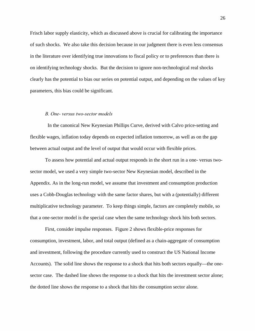
First, consider impulse responses. Figure 2 shows flexible-price responses for

consumption, investment, labor, and total output (defined as a chain-aggregate of consumption

and investment, following the procedure currently used to construct the US National Income

Accounts). The solid line shows the response to a shock that hits both sectors equally—the one-

sector case. The dashed line shows the response to a shock that hits the investment sector alone;

the dotted line shows the response to a shock that hits the consumption sector alone.

27

Note that the responses of output components to the two shocks are starkly different. The

investment-specific shock has most of the “standard” effects one expects in RBC models: output,

labor input and investment all rise. The only surprising result is that consumption falls, which is

due to the fact that our simple model has no adjustment costs of changing labor input, so in

response to an investment technology improvement the investment sector pulls labor out of the

consumption sector. On the other hand, consumption-specific shocks have basically no effect on

labor input and investment, and just raise consumption and output (and lower the relative price of

consumption goods, although this is not shown). In fact, BFFK (2008) show that if our model

had constant returns to scale in production and no distortions (e.g., from monopoly markups),

then consumption technology shocks would have precisely zero effect on labor and investment at

all horizons. BFFK emphasize that this “consumption technology neutrality” is an interesting

but little-known property of two-sector RBC models.

Figure 3 shows the corresponding impulse responses in the sticky-price model, where

monetary policy is assumed to follow a standard Taylor rule. We see that the two shocks have

effects on output and labor input that are qualitatively different: In the case of consumption

28

Figure 2: Flexible-price impulse responses

Notes: Units are percent deviations from steady-state. One-sector shock is an equal-sized change to both consumption and investment production technology.

technology shocks, output and labor input rise, by far more than in the flexible-price model, but

in the case of investment technology shocks, labor hours and output both fall. The differences

between the flexible- and sticky-price model are persistent—the output responses of the two do

29

not converge, even after 16+ quarters. Consumption-technology neutrality obviously no longer

holds, even as an approximation. The reason is that nominal price rigidity creates time-varying

Figure 3: Sticky-price impulse responses

Notes: Units are percent deviations from steady-state. One-sector shock is an equal-sized change to both consumption and investment production technology.

30

markups—which give rise to incentives to consume when goods are cheap and take leisure when

they are expensive that are missing in the flexible-price model, where markups are constant

over time. For similar reasons, investment-specific technology improvements lead to short-run

contractions in investment, output and labor input. Everyone knows that the prices of investment

goods will fall in the future, but they have not jumped down to their new flexible-price

equilibrium levels, since prices are a state variable. Since it is relatively easy to substitute

investment goods purchases intertemporally, the positive investment technology shock creates a

large short-run decline in investment demand, until prices have a chance to adjust.

These responses to the two types of technology shocks, while perhaps counter-intuitive,

match qualitatively the empirical estimates of BFFK (2008) on US data.

It is obvious from comparing Figures 2 and 3 that taking account of the two-sector nature

of production means that monetary policy has a much more complex job than in the one-sector

model, and the standard Taylor rule does not do a good job of stabilizing actual output relative to

potential. Ideally, monetary policy would work so that the impulse responses in Figure 3 are

identical to those in Figure 2. But for the monetary authority to take the appropriate action, it is

essential that policymakers know whether the shock is to consumption or investment technology.

With a consumption technology improvement, sticky-price output rises more than in the flexible-

price model; hence, monetary policy needs to be contractionary (relative to the prescriptions of

the standard Taylor rule). But when there is an investment-specific technology improvement,

monetary policy needs to be expansionary in order to avoid the slump that would otherwise

occur.

Second, we simulated the one- and two-sector models using the utilization-adjusted

technology shocks estimated in Fernald (2008). Table 4 shows standard deviations of selected

31

variables in flexible- and sticky-price versions of the one- and two-sector models, along with

actual data for the U.S. economy.

Table 4 Standard deviations, model simulations and data

Invest. Cons. Labor OutputOne-sector, flexible price 4.40 0.81 0.47 1.52Two-sector, flexible price 6.28 0.89 0.73 1.66One-sector, sticky price 4.82 0.84 0.64 1.60Two-sector, sticky price 5.52 0.87 0.85 1.68Data 4.54 1.12 1.14 1.95

Output gap (2-sector sticky less two-sector flex) 5.78 0.59 0.96 0.72"One-sector" estimated gap (2-sector sticky less 1-sect flex) 2.55 0.18 0.59 0.41

Notes: Model simulations use utilization-adjusted TFP shocks from Fernald (2008). Two-sector simulations use estimated quarterly consumption and investment technology; one-sector simulations use the same aggregate shock (a share-weighted average of the two sectoral shocks) in both sectors. All variables are filtered with the Christiano-Fitzgerald bandpass filter to extract variation between six and 32 quarters.

The model does a reasonable job of approximating the variation in actual data,

considering how simple it is and considering that we include just technology shocks. Investment

in the data is slightly less volatile than either sticky-price model or than either two-sector model.

That's not surprising, given that the model does not have any adjustment costs or other

mechanisms to smooth out investment. Consumption, labor and output in the data are more

volatile than in the models.23 Additional shocks (to government spending, monetary policy, or

preferences, say) would presumably add volatility to model simulations.

An important observation from Table 4 is that potential output—i.e., the flexible-price

simulations, in either the one- or two-sector variants—is highly variable, roughly as variable as

23 The relative volatility of consumption is not that surprising, actually, since the models do not have

consumer durables and we haven’t yet done the analysis for consumption of non-durables and services in the actual data.

32

sticky-price output. The short-run variability of potential output in New Keynesian models has

been emphasized by Nelson and Neiss (2005) and Edge, Kiley, and Laforte (2007).

In these models, with the shocks we’ve fed in, there’s a very high correlation of flexible-

and sticky-price output. In the two-sector case, the correlation is 0.91. Nevertheless, the implied

output gap (shown in the penultimate line of Table 4 as the difference between output in the

sticky- and flexible-price cases) is more volatile than would be implied if one estimated potential

output using the one-sector model (the final line).

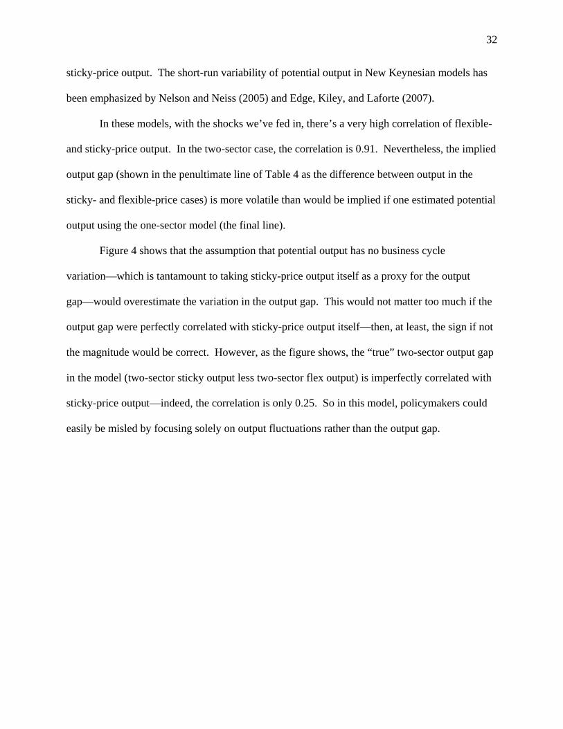
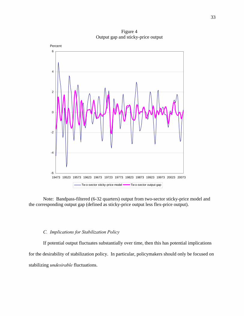
Figure 4 shows that the assumption that potential output has no business cycle

variation—which is tantamount to taking sticky-price output itself as a proxy for the output

gap—would overestimate the variation in the output gap. This would not matter too much if the

output gap were perfectly correlated with sticky-price output itself—then, at least, the sign if not

the magnitude would be correct. However, as the figure shows, the “true” two-sector output gap

in the model (two-sector sticky output less two-sector flex output) is imperfectly correlated with

sticky-price output—indeed, the correlation is only 0.25. So in this model, policymakers could

easily be misled by focusing solely on output fluctuations rather than the output gap.

33

Figure 4 Output gap and sticky-price output

Note: Bandpass-filtered (6-32 quarters) output from two-sector sticky-price model and the corresponding output gap (defined as sticky-price output less flex-price output).

C. Implications for Stabilization Policy

If potential output fluctuates substantially over time, then this has potential implications

for the desirability of stabilization policy. In particular, policymakers should only be focused on

stabilizing undesirable fluctuations.

-6

-4

-2

0

2

4

6

19473 19523 19573 19623 19673 19723 19773 19823 19873 19923 19973 20023 20073

Tw o-sector sticky-price model Tw o-sector output gap

Percent

34

Of course, the welfare benefits of such policies remain controversial. Lucas (1987, 2003)

famously argued that, given the fluctuations we observe, the welfare gains from additional

stabilization of the economy is likely to be small. In particular, given standard preferences and

the observed variance of consumption (around a linear trend), a representative consumer would

be willing to reduce his average consumption by only about ½ of 1/10th of one percent in

exchange for eliminate all remaining variability in consumption. Note that this calculation does

not necessarily imply that stabilization policy doesn’t matter, since the calculation takes as given

the stabilization policies that were implemented in the past. Stabilization policies might well

have been valuable—e.g., in eliminating recurrences of the Great Depression, or by minimizing

the frequency of severe recessions—but additional stabilization might not offer large benefits.

This calculation amounts to some $5 billion per year in the United States, or about $16

per person. Compared with the premiums we pay for very partial insurance (e.g., for collision

coverage on our cars), this is almost implausibly low. Any politician would surely vote to pay

$5 billion for a policy that would eliminate recessions.

Hence, a sizeable literature considers ways to obtain larger costs of business-cycle

fluctuations, with mixed results. Arguments in favor of stabilization include Galí, Gertler, and

López-Salido (2007), who argue that the welfare effects of booms and recessions may be

asymmetric. In particular, because of wage and price markups, steady-state employment and

output are inefficiently low in their model, so that the costs of fluctuations depend on how far the

economy is from full employment. Recessions are particularly costly—welfare falls by more

during a business-cycle downturn than it rises during a symmetric expansion. Barlevy (2004)

argues in an endogenous-growth framework that stabilization might increase the economy’s

35

long-run growth rate, allowing him to obtain very large welfare effects from business-cycle

volatility.

This discussion of welfare effects highlights that much work remains to be done to

understand the desirability of observed fluctuations; the ability of policy to smooth the

undesirable fluctuations in the output gap; and the welfare benefits of such policies.

IV. What is current potential output growth?

Consider the current situation, as of late 2008: Is potential output growth relatively high,

relatively low, or close to its steady-state value?24 The answer is important for policymakers,

where statements by the Federal Open Market Committee (FOMC) participants have emphasized

the importance of economic weakness in reducing inflationary pressures.25 Moreover, a

discussion of the issue highlights some of the issues of what we know, and do not know, about

potential output. Some of the considerations are closely linked to earlier points we have made;

but these considerations also allow a discussion of other issues that aren’t in the simple models

we’ve discussed.

Several arguments suggest that potential output growth might currently be running at a

relatively rapid pace. First, and perhaps most importantly, total factor productivity growth has

been relatively rapid from the end of 2006 through the third quarter of 2008 (see Table 2). This

has been a period when output growth itself was relatively weak, and hours per worker were

generally falling; hence, following the logic in BFK, factor utilization appears to have been

falling, as well. As a result, in both the consumption and the investment sectors, utilization-

24 We could, equivalently, discuss the magnitude or even sign of the output gap, which is naturally defined

in levels. The level is the integral of the growth rates, of course, and growth rates make it a little easier to focus, at least implicitly, on how the output gap is likely to change over time.

25 For example, in the minutes from the September 2008 FOMC meeting, participants forecast that over time, “…increased economic slack would tend to damp inflation.” /www.federalreserve.gov/monetarypolicy/fomcminutes20080916.htm.

36

adjusted TFP, from Fernald (2008), has grown at a more rapid pace than its post-1995 average.

This fast pace has occurred despite the reallocations of resources away from housing and finance

and the high level of financial stress.

Second, substantial declines in wealth are likely to increase desired labor supply. Most

obviously, housing wealth has fallen and stock-market values have plunged; but tax and

expenditure policies aimed at stabilizing the economy could also suggest a higher present value

of taxes. Declining wealth has a direct, positive effect on labor supply. In addition, as the logic

of Campbell and Hercowitz (2006) would imply, rising financial stress could lead to increases in

labor supply as workers need to acquire larger down-payments for purchases of consumer

durables. And if there is habit-persistence in consumption, workers might also temporarily

increase desired labor effort in order to smooth the effects of shocks to gasoline and food prices.

Nevertheless, there are also reasons to be concerned that potential output growth is

currently lower than its pace over the past decade or so. First, Phelps (2008) raises the

possibility that because of a sectoral shift away from housing-related activities and finance,

potential output growth is temporarily low and the natural rate of unemployment is temporarily

high. Although qualitatively suggestive, it is unclear that the sectoral shifts argument is

quantitatively important. For example, Valletta and Cleary (2008) look at the (weighted)

dispersion of employment growth across industries, a measure used by Lilien (1982). They find

that as of the third quarter of 2008, “the degree of sectoral reallocation…remains low relative to

past economic downturns.” Valletta and Cleary also look at job-vacancy data, which Abraham

and Katz (1986) suggest could help distinguish between sectoral shifts and pure cyclical

increases in unemployment and employment dispersion. The basic logic is that in a sectoral-

shifts story, expanding firms should have high vacancies that partially or completely offset the

37

low vacancies in contracting firms. Since late 2006, Valletta and Cleary find that the vacancy

rate has been steadily falling.26

Second, Bloom (2008) argues that uncertainty shocks are likely to lead to a sharp decline

in output. As he puts it, there has been “…a huge surge in uncertainty that is generating a rapid

slow-down in activity, a collapse of banking preventing many of the few remaining firms and

consumers that want to invest from doing so, and a shift in the political landscape locking in the

damage through protectionism and anti-competitive policies.” His argument is based on the

model simulations in Bloom (2007), in which an increase in macro uncertainty causes firms to

temporarily pause investment and hiring. In his model, productivity growth also falls temporarily

because of reduced reallocation from lower to higher productivity establishments.

Third, along the lines suggested by Bloom (2007) as well as by Eisfeldt and Rampini

(2006), the credit freeze could directly reduce productivity-improving reallocations. Eisfeldt and

Rampini argue that, empirically, capital reallocation is procyclical, whereas the benefits

(reflecting cross-sectional dispersion of marginal products) are countercyclical. These

observations suggest that the informational and contractual frictions, including financing

constraints, are higher in recessions. The situation as of late 2008 is one in which financing

constraints are particularly severe, which is likely to reduce efficient reallocations of both capital

and labor.

Fourth, there could be other effects from the seizing-up of financial markets in 2008.

Financial intermediation is an important intermediate input into production in all sectors. If it is

complementary with other inputs (as in Jones, 2008)—e.g., you need access to the commercial

26 Valletta and Cleary do find some evidence that the U.S. Beveridge curve might have shifted out in recent

quarters relative to its position from 2000 to 2006.

38

paper market in order to finance working capital needs—then it could lead to substantial

disruptions of real operations.

Finally, the substantial volatility in commodity prices, especially oil, in recent years

could affect potential output. That said, although oil is a crucial intermediate input into

production, changes in oil prices do not have a clear-cut effect on TFP, measured as domestic

value added relative to primary inputs of capital and labor. They might, nevertheless, affect

equilibrium output by affecting equilibrium labor supply. Blanchard and Gali (2007) and

Bodenstein, Erceg, and Guerrieri (2008), however, are two recent analyses in which, because of

(standard) separable preferences, there is no effect on flexible-price GDP or employment from

changes in oil prices. So there is no a priori reason to expect fluctuations in oil prices to have a

substantial effect on the level or growth rate of potential output.

A difficulty for all of these arguments that potential output growth might be temporarily

low is the observation already made, that productivity growth (especially after adjusting for

utilization) has, in fact, been relatively rapid over the past seven quarters.

It is possible the productivity data have been mismeasured in recent quarters.27 Basu,

Fernald, and Shapiro (2001) highlight variations in disruption costs associated with tangible

investment. Comparing 2004:Q4-2006:Q4 (when productivity growth was weak) to 2006:Q4-

2008:Q3 (when productivity was strong), growth in business fixed investment was very similar,

suggesting that time-varying disruption costs probably explains little of the recent variation in

productivity growth rates.

27 Note also that the data are all subject to revision. For example, the annual revision in 2009 will revise

data back to the beginning of 2006. In addition, labor-productivity data for the non-financial corporate sector, which is based on income-side rather than expenditure-side data, shows less of a slowdown in 2005 and 2006, and less of a pickup since then. That said, even the non-financial corporate productivity numbers have remained relatively strong in the past few years.

39

Basu, Fernald, Oulton, and Srinivasan (BFOS, 2003) and Oliner, Sichel, and Stiroh

(2007) discuss the role of mismeasurement associated with intangible investments, such as

organizational changes associated with information technology. With greater concerns about

credit and cash flow, firms might have deferred organizational investments and reallocations; in

the short run, such deferral would imply faster measured productivity growth, even if true

productivity growth (in terms of total output, the sum of measured output plus unobserved

intangible investment) were constant. BFOS argue for a link between observed investments in

computer equipment and unobserved intangible investments in organizational change. Growth in

computer and software investment does not show a notable difference between the 2004:Q4-

2006:Q4 period and the 2006:Q4-2008:Q2 period—and, if anything, the investment rate was

higher in the latter period—so that this proxy again does not imply mismeasurement.

Given wealth effects on labor supply, strong recent productivity performance—along

with the failure of typical proxies for mismeasurement to explain the productivity performance—

therer are reasons for optimism about the short-run pace of potential output growth.

Nevertheless, the major effects of the adverse shocks on potential output seem likely to be ahead

of us. For example, the widespread seizing-up of financial markets has been especially

pronounced only in the second half of 2008. We expect that as the effects of the collapse in

financial intermediation, the surge in uncertainty, and the resulting declines in factor reallocation

play out over the next several years, short-run potential output growth will be constrained

relative to where it otherwise would be.

V. Conclusions

This paper has highlighted a few things we think we know about potential output--

namely, the importance in both the short run and the long run of rapid technological change in

40

producing equipment investment goods; and the likely time-variation in the short-run growth rate

of potential. Our discussion of these points has, of course, pointed towards some of the many

things we don’t know.

Taking a step back, we have advocated thinking about policy in the context of explicit

models that suggest ways to think about the world, including potential output. But there is an

important interplay between theory and measurement, as the discussion suggests. Every day,

actual policymakers grapple with challenges that aren’t present in the standard models. Not only

do they not know the true model of the economy, but they don’t know the current state variables

or the shocks with any precision; and the environment is potentially nonstationary, with the

continuing question of whether structural change (e.g., parameter drift), has occurred. Theory

(and practical experience) tell us that our measurements are imperfect, particularly in real time.

Not surprisingly, central bankers look at a lot of real-time indicators, and filter them

analytically—relying on theory and experience. Estimating potential output growth is one

modest and relatively transparent example of this interplay between theory and measurement.

41

Appendix: A Simple Two Sector Sticky Price Model28

1 Households The economy is populated by a representative household which maximizes its lifetime

utility

0=0

( , )t tt

maxE u C L∞

∑

where tC is consumption of a CES basket of differentiated varieties

1 11

0= ( )tC C z dz

ξξ ξξ− −⎡ ⎤

⎢ ⎥⎢ ⎥⎣ ⎦∫ and tL is labor effort. u, the period felicity function, takes the following

form:

1

=1

tt t

Lu lnCη

η

+

−+

where η is the inverse of the Frisch elasticity of labor supply. The maximization problem

is subject to several constraints. The flow budget constraint, in nominal terms, is the following: 1 1 1= (1 )I C

t t t t t t t t t t tB P I P C W L R K i B− − −+ + + + + + Δ

where 1 11

0= ( )I I z dz

ξξ ξξ− −⎡ ⎤

⎢ ⎥⎢ ⎥⎣ ⎦∫ . The price indexes are defined as follows:

( )1

1 11

0= ( )C C

t tP P z dz ξξ −−∫

( )1

1 11

0= ( )I I

t tP P z dz ξξ −−∫

Moreover, we have 1= (1 )t t tK I Kδ −+ − (1) = C I

t t tL L L+ (2) 1 = C I

t t tK K K− + (3) Notice that total capital is predetermined, while sector-specific capital are free to move in

each period. In order to solve the problem, let's write the Lagrangian as: 28 Written primarily by Alessandro Barattieri.

42

( )1

1 1 1= ... (1 )1

I Ctt t t t t t t t t t t t t t

LL lnC B P I P C W L R K i Bη

η

+

− − −− + −Λ + + − − − + −Δ+

( )1 1 1 1 1 1 1 1 1 1(1 ) ...I Ct t t t t t t t t t t t t tE B P I P C W L R K i Bβ + + + + + + + + + +− Λ + + − − − + −Δ −

The f.o.c. of the maximization problem for consumption, nominal bond, labor and capital are as follows:

1 = Ct t

t

PC

Λ (4)

[ ]1= (1 )t t t tE iβ +Λ + Λ (5)

= t tL wη Λ (6)

( )1 1 1= (1 )I It t t t t tP E R Pβ δ+ + +

⎡ ⎤Λ Λ + −⎣ ⎦ (7)

2 Firms Both sectors are characterized by a unitary mass of atomistic monopolistically

competitive firms. Production functions are Cobb-Douglas (possibly with different factor intensities). Productivity in the two sectors is represented by two AR(1) processes. The cost minimization problems for the firms z operating in the consumption and investment sectors can be expressed, in nominal terms, as follows:

Min ( ) ( )C C

t t t tW L z R K z+ s.t. 1( ) = ( ( )) ( ( ))C CC C C C C

t t t tY z A K z L zα α− −Φ and analogously: Min ( ) ( )I I

t t t tW L z R K z+ s.t. 1= ( ( )) ( ( ))I II I I I

t t t tI A K z L zα α− −Φ calling iμ with = ,i C I the multiplier attached to the minimization problem, reflecting

nominal marginal cost, we can express the factor demand as follows, where we omit z assuming a symmetric equilibrium:

= (1 ) ( ) ( )C CC C Ct

t t tCt

W A K Lα ααμ

−−

1 1= ( ) ( )C CC C Ct

t t tCt

R A K Lα ααμ

− −

= (1 ) ( ) ( )I II I It

t t tIt

W A K Lα ααμ

−−

1 1= ( ) ( )I II I It

t t tIt

R A K Lα ααμ

− −

Taking the ratio for each sector, we get

43

=1

Ct tCt t

K WL R

αα−

(8)

=1

It tIt t

K WL R

αα−

(9)

Inflation rates are naturally defined as

1

=j

j tt j

t

PP−

Π (10)

Finally, given the Cobb-Douglas assumption, it is possible to express the nominal

marginal cost as follows:

11 1= ( )( )

j j jjMC R W Y

A fα α

α− +Φ (11)

with = ,j C I . We introduce nominal rigidities through standard Calvo (1983) pricing. Instead of

writing the rather complex equations for the price levels in the C and I sectors, we jump directly to the log-linearized Calvo equations for the evolution of inflation rates, equations (25) and (26) below.

3 Monetary Policy Monetary policy is conducted through a Taylor-type rule with a smoothing parameter and

reaction to inflation and marginal cost. Again, we write the Taylor rule directly in log-linearized form, as equation (32) below.

4 Equilibrium Beyond the factor market clearing conditions already expressed before, equilibrium

requires also a bond market clearing condition ( = 0B ), a consumption-goods market clearing condition ( =CY C ) and an aggregate adding up condition ( =C I Y+ ). (By Walras’s law, we drop the investment-market clearing condition.)

5 The Linearized model The equations of the model linearized around its non-stochastic steady state are

represented by eq 12-36, which are 25 equation in the 25 unknown endogenous variables , , , , , , ,I C C Ic l l l k k k , , , , , , , , ,C C I Cw w r i y I y p pλ , , , , , , ,C I I C C Ia aπ π π μ μ μ

1= (1 )t t tk I kδ δ −+ − (12)

44

=I C

I Ct t t

L Ll l lL L

+ (13)

1=I C

I Ct t t

K Kk k kK K −+ (14)

= Ct t tc pλ− + (15)

1=t t tiλ λ ++ (16) = t tl wη λ + (17) [ ]1 1 1= 1 (1 ) (1 )I I

t t t t tp r pλ λ β δ β δ+ + ++ + − − + − (18)

( )= (1 )C C C C C C Ct t t ty a k lα αΓ + + − (19)

( )= (1 )I I I I I It t t tI a k lα αΓ + + − (20)

=C Ct t t tk r w l+ + (21)

=I It t t tk r w l+ + (22)

= (1 )C Ct t t tr w aμ α α+ − − (23)

= (1 )I It t t tr w aμ α α+ − − (24)

1= ( )C C C Ct t t pπ βπ ζ μ+ + − (25)

1= ( )I I I It t t pπ βπ ζ μ+ + − (26)

1=C C Ct t tp pπ −− (27)

1=I C It t tp pπ −− (28)

= _ _C It t tC share INV shareμ μ μ+ (29)

= _ _C It t tC share INV shareπ π π+ (30)

=C Ct t tw w p− (31)

1= (1 )( )t i t i t t ti i π μρ ρ φ π φ μ ν− + − + + (32) = _ _t t ty C sharec INV shareI+ (33) =C

t ty c (34) 1=C C C

t C t ta aρ ε− + (35) 1=I I I

t I t ta aρ ε− + (36)

45

Table 1: Baseline Calibration Parameter Value

β 0.99 η 0.25

Cα 0.3

Iα 0.3 δ 0.025

CΓ 1.1 IΓ 1.1

Cθ 0.75

Iθ 0.75

Cζ (1 )(1 )C C

C

θ βθθ

− −

Iζ (1 )(1 )I I

I

θ βθθ

− −

_INV SHARE 0.2 _C SHARE 0.8

ILL

0.2

CLL

0.8

IKK

0.2

CKK

0.8

iρ 0.8

πφ 1.5

μφ 0.5

Cρ 0.99

Iρ 0.99

Ctε

σ 1

Itε

σ 1

tνσ 1

46

Bibliography

Congressional Budget Office (2001). “CBO’s Method for Estimating Potential Output: An Update. 2001. Technical report, Congressional Budget Office.

Congressional Budget Office (2004). A Summary of Alternative Methods for Estimating Potential GDP. 2004. Technical report, Congressional Budget Office.

Congressional Budget Office (The Budget and Economic Outlook: An Update. Technical report, 2008.

Survey of Professional Forecasters. Technical report, Federal Reserve Bank of Philadelphia, 2008.

Abraham, Katharine G. and Lawrence F. Katz. “Cyclical Unemployment: Sectoral Shifts or Aggregate Disturbances?” 1986. The Journal of Political Economy 94: 507–522.

Alexopoulos, Michelle. “Read all about it! ! What happens following a technology shock?” 2006.

Barlevy, Gadi. “On the Timing of Innovation in Stochastic Schumpeterian Growth Models.” 2004. National Bureau of Economic Research Working Paper Series: 10741+.

Basu, Susanto, John Fernald, and Miles Kimball. “Long-Run Labor Supply and the Elasticity of Intertemporal Substitution for Consumption.” 2002.

Basu, Susanto, John G. Fernald, Nicholas Oulton, and Sylaja Srinivasan. “The Case of the Missing Productivity Growth: Or, Does Information Technology Explain Why Productivity Accelerated in the United States but Not the United Kingdom?” 2003.

Basu, Susanto and John G. Fernald. “Returns to Scale in U.S. Production: Estimates and Implications.” 1997. The Journal of Political Economy 105: 249–283.

Basu, Susanto and John G. Fernald. “Aggregate productivity and aggregate technology.” 2002. European Economic Review 46: 963–991.

Basu, Susanto, John G. Fernald, and Miles S. Kimball. “Are Technology Improvements Contractionary?” 2006. The American Economic Review 96: 1418–1448.

Basu, Susanto, John G. Fernald, and Matthew D. Shapiro. “Productivity growth in the 1990s: technology, utilization, or adjustment?” 2001. Carnegie-Rochester Conference Series on Public Policy 55: 117–165.

Basu, Susanto, John Fernald, Jonas Fisher, and Miles Kimball. “Sector-Specific Technical Change.” Manuscript, 2008.

Blanchard, Olivier J. and Jordi Gali. “The Macroeconomic Effects of Oil Price Shocks: Why are the 2000s so Different from the 1970s?” 2007. MIT Department of Economics Working Paper 07.

Bloom, Nicholas. “The Impact of Uncertainty Shocks.” 2007. National Bureau of Economic Research Working Paper Series: 13385+.

Bloom, Nicholas. The Credit Crunch May Cause Another Great Depression. 2008. Bodenstein, Martin, Christopher J. Erceg, and Luca Guerrieri. “Optimal Monetary Policy

with Distinct Core and Headline Inflation Rates.” 2008. Social Science Research Network Working Paper Series.

47

Bureau of Labor Statistics (2008). Multifactor Productivity data. Downloaded from www.bls.gov.

Campbell, Jeffrey R. and Zvi Hercowitz. “The Role of Collateralized Household Debt in Macroeconomic Stabilization.” 2005. National Bureau of Economic Research Working Paper Series: 11330+.

Card, David. “Intertemporal Labor Supply: An Assessment.” 1991. National Bureau of Economic Research Working Paper Series: 3602+.

Christiano, Lawrence J. and Terry J. Fitzgerald. “The Band Pass Filter.” 1999. National Bureau of Economic Research Working Paper Series: 7257+.

Delong, Bradford J. Productivity Growth in the 2000s. March 2002. Edge, Rochelle M., Michael T. Kiley, and Jean-Philippe Laforte. “Natural Rate Measures in

an Estimated DSGE Model of the U.S. Economy.” 2007. FEDS Working Paper. Eisfeldt, Andrea and Adriano Rampini. “Capital reallocation and liquidity.” April 2006.

Journal of Monetary Economics 53: 369–399. Elsby, Michael and Matthew Shapiro. Stepping Off the Wage Escalator: A Theory of the

Equilibrium Employment Rate. 2008. Fernald, John G. “A Quarterly Utilization-Adjusted Measure of Total Factor Productivity.”

2008. Fisher, Jonas D. M. “The Dynamic Effects of Neutral and Investment-Specific Technology

Shocks.” 2006. The Journal of Political Economy 114: 413–451. Gali, Jordi, Mark Gertler, and David J. Lopez-Salido. “Markups, Gaps, and the Welfare

Costs of Business Fluctuations.” November 2007. The Review of Economics and Statistics 89: 44–59.

Gordon, Robert J. The Measurement of Durable Goods Prices (National Bureau of Economic Research Monograph). 1990. University Of Chicago Press.

Gordon, Robert J. “Does the "New Economy" Measure up to the Great Inventions of the Past? ” 2000. The Journal of Economic Perspectives 14: 49–74.

Gordon, Robert J. “Future U.S. Productivity Growth: Looking Ahead by Looking Back.” 2006.

Greenwood, Jeremy, Zvi Hercowitz, and Per Krusell. “Long-Run Implications of Investment-Specific Technological Change.” 1997. The American Economic Review 87: 342–362.

Hansen, Gary D. “Indivisible labor and the business cycle.” 1985. Journal of Monetary Economics 16: 309–327.

Jones, Charles I. “R & D-Based Models of Economic Growth.” 1995. The Journal of Political Economy 103: 759–784.

Jones, Charles I. “Sources of U.S. Economic Growth in a World of Ideas.” 2002. The American Economic Review 92: 220–239.

Jones, Charles I. “Intermediate Goods, Weak Links, and Superstars: A Theory of Economic Development.” March 2008. National Bureau of Economic Research Working Paper Series: 13834+.

Jorgenson, Dale Productivity and Economic Growth. 1992. University Of Chicago Press.

48

Jorgenson, Dale W. “Information Technology and the U.S. Economy.” 2001. The American Economic Review 91: 1–32.

Jorgenson, Dale W., Mun Ho, and Kevin J. Stiroh, 2008. "A Retrospective Look at the U.S. Productivity Growth Resurgence.” Journal of Economic Perspectives, 22:1 pp3-24.

Justiniano, Alejandro and Giorgio Primiceri. “Potential and Natural Output.” 2008. King, Robert G., Charles I. Plosser, and Sergio T. Rebelo. “Production, growth and business

cycles : I. The basic neoclassical model.” 1988. Journal of Monetary Economics 21: 195–232.

Kuttner, Kenneth N. “Estimating Potential Output as a Latent Variable.” 1994. Journal of Business and Economic Statistics 12: 361–368.

Kydland, Finn E. and Edward C. Prescott. “Rules Rather than Discretion: The Inconsistency of Optimal Plans.” 1977. The Journal of Political Economy 85. 473–492.

Laubach, Thomas and John C. Williams. “Measuring the Natural Rate of Interest.” 2003. The Review of Economics and Statistics 85: 1063–1070.

Lilien, David M. “Sectoral Shifts and Cyclical Unemployment.” 1982. The Journal of Political Economy 90: 777–793.

Lucas, Robert E. “Econometric policy evaluation: A critique.” 1976. Carnegie-Rochester Conference Series on Public Policy 1: 19–46.

Lucas, Robert E. Models of Business Cycles (Yrjo Jahnsson Lectures). 1991. Wiley-Blackwell.

Lucas, Robert E. “Macroeconomic Priorities.” 2003. The American Economic Review 93: 1–14.

Neiss, Katharine S. and Edward Nelson. “Inflation Dynamics, Marginal Cost, and the Output Gap: Evidence from Three Countries.” 2005. Journal of Money, Credit and Banking 37: 1019–1045.

Okun, Arthur M. The Political Economy of Prosperity. 1970. 1st edition. W. W. Norton & Company.

Oliner, Stephen D. and Daniel E. Sichel. “The Resurgence of Growth in the Late 1990s: Is Information Technology the Story?” 2000. The Journal of Economic Perspectives 14: 3–22.

Phelps, Edmund S. “U.S. Monetary Policy and the Prospective Structural Slump.” June 2008.

Ramsey, Frank P. “A Mathematical Theory of Saving.” 1928. The Economic Journal 38: 543–559.

Rogerson, Richard. “Indivisible labor, lotteries and equilibrium.” 1988. Journal of Monetary Economics 21: 3–16.

Rotemberg, Julio J. “Stochastic Technical Progress, Nearly Smooth Trends and Distinct Business Cycles.” 2002. National Bureau of Economic Research Working Paper Series: 8919+.

Sichel, Daniel E. and Stephen D. Oliner. “Information Technology and Productivity: Where are We Now and Where are We Going? .” 2002. Social Science Research Network Working Paper Series.

49

Smets, Frank and Rafael Wouters. “Shocks and Frictions in US Business Cycles: A Bayesian DSGE Approach.” (June 2007). American Economic Review 97: 586–606.

Solow, Robert M. “A Contribution to the Theory of Economic Growth.” The Quarterly Journal of Economics 70 (1956): 65–94.

Solow, Robert M. “Is There a Core of Usable Macroeconomics We Should All Believe In?” (1997). The American Economic Review 87: 230–232.

Tosetto, Elena. Revisions of Quarterly Output Gap Estimates for 15 OECD Member Countries. 2008. Technical report, OECD / Statistics Directorate.

Valletta, Rob and Aisling Cleary. “Sectoral Reallocation and Unemployment.” 2008. Economic Letter.

Violante, Giovanni L. and Jason G. Cummins. “Investment-Specific Technical Change in the United States (1947-2000): Measurement and Macroeconomic Consequences.” (April 2002). Review of Economic Dynamics 5 :243–284.

Whelan, Karl. “Real Wage Dynamics and the Phillips curve.” (2000). Finance and Economics Discussion Series 2000-02.

Whelan, Karl. “A Two-Sector Approach to Modeling U.S. NIPA Data.” 2003. Journal of Money, Credit and Banking 35: 627–656.