What Caused Chicago Bank Failures in the Great Depression ... · 1930 points to a powerful...

What Caused Chicago Bank Failures in the Great Depression? A

Look at the 1920s

Natacha Postel-Vinay∗

Department of Economic HistoryLondon School of Economics

London, WC2A [email protected]

June 2013

Abstract

This paper reassesses the causes of Chicago bank failures during the Great Depressionby tracking the evolution of their balance sheets in the 1920s. Looking at the long-termbehaviour of financial ratios from 1923 to 1933 provides new insights into the causes of bankfailures. Using multinomial logistic regression analysis by cohort, I find that banks whichfailed the earliest in the 1930s had invested more in non-liquid assets (in particular, mort-gages) in the 1920s. However, all Chicago banks suffered tremendous deposit withdrawalsduring 1930-1933 in what seems to have been an indiscriminate run. The main cause ofbank failure was therefore a combination of illiquid mortgages on the asset side and depositlosses on the liability side. Banks heavily engaged in mortgages did not have enough liquidassets to face the withdrawals and failed.

JEL- Classification: G11, G21 and N22Keywords: Great Depression, Commercial Banks, Portfolio Choice and Mortgage

∗I am very grateful to my advisors Olivier Accominotti and Albrecht Ritschl for their continuous supportand guidance. I would also like to thank Mark Billings, Mark Carlson, Barry Eichengreen, Alexander Field,John Gent, Steve Gjerstad, Frank Kennedy, Joe Mason, Kris Mitchener, Anne Murphy, Jonathan Rose, MarkTippett, Stephan Werner, Eugene White and seminar participants at the London School of Economics, QueensUniversity Belfast, the Canadian Network of Economic Historians Conference in Banff, the Economic HistorySociety Annual Conference in York, the Cliometrics Workshop in Strasbourg, and the Economic and BusinessHistory Society Conference in Baltimore. Funding from the Economic and Social Research Council is gratefullyacknowledged. All errors are mine.

1

1 Introduction

Recently, a number of researchers have linked bank failures in the U.S. Great Depression to

fundamental weaknesses already apparent just before the start of the depression, around June

1929 (Calomiris & Mason, 1997, 2003; Guglielmo, 1998; White, 1984). According to this view,

depositors ran on banks because they were insolvent, therefore causing them to fail. This view

apparently contrasts with the one pioneered by Friedman & Schwartz (1963) in which all banks

faced very large, non-discriminating withdrawals, which caused even healthy banks to fail. This

paper shows how these two interpretations may be reconciled. I find that banks that failed the

earliest in Chicago had invested more in non-liquid assets (in particular, mortgages) as early as

1923. However, all banks suffered tremendous withdrawals during the depression in what could

be described as a general, non-discriminating run. The run therefore revealed which banks

heavily engaged in mortgage investments during the 1920s by causing them to fail.

Chicago area banks suffered one of the highest failure rates in the US, especially in the first

halves of 1931 and 1932.1 Indeed, out of 193 state banks in June 1929, only 35 survived up to

June 1933. For this reason Chicago has often been the subject of banking studies (Calomiris &

Mason, 1997; Esbitt, 1986; Guglielmo, 1998; Thomas, 1935).

Yet my analysis departs from previous research along two dimensions. First, I introduce

a novel way of examining Chicago state bank failures by separating them into three cohorts:

June 1931 failures, June 1932 failures and June 1933 failures, each corresponding to six-month

failure windows containing both panic and non-panic failures. Key variables such as return on

equity, reserve-deposit ratios and real estate loan shares are compared between the four cohorts.

Second, rather than focusing on banks’ 1929 balance sheets, I look at the evolution of survivors

and failures during the full decade from 1923 all the way up to 1933.

The main finding of this paper is that the banks failing early in the depression were those

which had heavily invested in non-liquid assets – especially in mortgages – as early as 1923. In

particular, several banks had significantly invested in real estate loans not only throughout the

1920s, but especially from 1928 onwards – particularly the first two failure cohorts. The ratio of

mortgages to total assets is also the best predictor of time of failure. June 1933 failures behaved

in general more erratically throughout the decade. Many other bank characteristics explain

1Chicago had the highest failure rate of any urban area (Guglielmo, 1998).

2

failure as early as 1923 (such as retained earnings to net worth), although not as consistently

and not to the same degree as real estate loans.

I also look at deposit withdrawals to examine what kind of run (discriminating or not) each

cohort faced in their preceding non-panic window, and whether withdrawals were determined

by mortgage investments or not. Overall, I find that all banks faced tremendous withdrawals,

despite the significant differences between them in terms of mortgage investments. In the first

failure episode (1931), which saw the largest number of failures, depositors did not identify

these banks as particularly weak even in the preceding non-panic window, although out of all

banks these held the highest share of real estate loans. Indeed, in this first episode all banks lost

tremendous amounts of deposits, but the failing banks did not lose significantly more than the

others, and their deposit losses are not well explained by their share of mortgages. In the second

episode (1932) the picture changed somewhat: the banks that failed did lose more deposits than

survivors, and mortgages are the main predictor of withdrawals in the year preceding failure.

Nevertheless, survivors lost a tremendous amount of deposits as well (around 37 per cent), and

it is not clear whether the differential in deposit losses can be taken as an important cause of

failure. Thus, while underlining the significant role of the mortgage share of a bank’s assets

in its failure, this paper re-asserts the importance of non-discriminating withdrawals in the

preceding non-panic window. Banks heavily engaged in mortgages did not have enough liquid

assets to face the withdrawals and failed.

It is not the aim of this paper to determine the exact cause of these indiscriminate with-

drawals. There is a large literature on the causes of bank runs. Diamond & Dybvig (1983)

see them as undesirable equilibria in which borrowers observe a sunspot and withdraw their

deposits, thus causing even “healthy” banks to fail. On the other hand, Calomiris & Gorton

(1991) and Calomiris & Kahn (1991) see bank runs as a form of monitoring: unable to costlessly

value banks’ assets, borrowers observing a specific shock to those assets use runs to reveal the

weakest banks. This view is closer to the one developed in this paper, in that withdrawals

revealed which banks had the most illiquid assets. Yet whether depositors observed a specific

shock or not remains to be seen.

This paper emphasizes the importance of mortgages’ sheer lack of liquidity as a determinant

risk factor. A decline in home prices and mortgage losses may have mattered, but they are not

3

needed to drive the explanation given in this paper. The view that illiquid assets were the

cause of the crisis is supported by evidence that all banks engaged in fire sales. In this process,

mortgages could not be liquidated. Indeed, given the absence of a developed secondary market,

real estate loans increased as a share of total assets for all banks during the depression, at the

same time as assets as a whole were declining.2 Other types of loans, such as loans on collateral

security and “other loans,” were promptly liquidated.

Such results suggest a reassessment of the role of real estate in the Great Depression. Chicago

is well-known for its real estate boom in the 1920s, one that resembled both in character and

magnitude the suburban real estate booms of some of the major cities of the American East

North Central and Middle-Atlantic regions.3 Given that the former region had one of the

highest numbers of suspensions in the U.S., the close connection between bank failures and the

real estate booms seems worth investigating.4 The link between real estate and the depression

is probably not a direct one, in the sense that the direct contribution of real estate to the

decline in economic activity was small. A number of recent papers have demonstrated that, in

the aggregate, the role of real estate in the Great Depression was indeed minor.5 This paper

assesses the indirect, probably larger contribution that real estate made to the deepening of the

Great Depression via the banking channel. Analysis of the second largest city in the U.S. in

1930 points to a powerful relationship between real estate lending and commercial bank failures

in the Great Depression.6

Section two reviews the literature on banks fundamental troubles during the U.S. Great

Depression. Section three introduces the data and empirical approach adopted in this study.

Section four presents results for the 1920s, focusing on all available variables except deposit

losses, and provides a historical explanation for Chicago bank behaviour in the 1920s. Section

five analyses the impact of deposit losses at the time of failure. Section six concludes.

2Mortgage securitization by Chicago state banks was rudimentary at best and mostly limited regionally,preventing broader diversification of risk. See Goetzmann & Newman (2010) and Postel-Vinay (2013a).

3These were commonly used census regions. The Chicago boom can be compared in particular to those ofDetroit, Pittsburgh, Philadelphia (see Wicker, 1996, pp. 16,18), and Toledo (Messer-Kruse, 2004). See also Allen(1931).

4The East North Central region (which contains Chicago) had 2,770 suspensions in total between 1930 and1933 (the term suspension refers to temporary or permanent bank failure, as opposed to failure which refers onlyto the latter category). Only the agricultural states of the West North Central region surpass this number witha total of 3,023 suspensions (Board of Governors of the Federal Reserve System, 1937, p. 868). Note that thestate of Pennsylvania also had a particularly high failure rate (ibid.).

5See, in particular, White (2009), and Field (2013).6Chicago was home to 3,376,438 dwellers in 1930, as compared to New York Citys population of 6,930,446

(Carter et al., 2006, Series Aa1-5).

4

2 Literature Review

When economic historians first started to look more deeply into the causes of Great Depression

bank failures, and in particular at whether more “fundamental” causes existed than mass deposit

withdrawals (Friedman & Schwartz, 1963), they mainly focused on the condition of banks

right before the start of the depression, around June 1929. The idea was that if it could be

demonstrated that failures showed particular weaknesses before the start of the slump this

meant that their fundamentals were impaired, which explained their later failure. A number of

authors argue that these banks had been suffering from weak loans and investments before they

failed, and that there is little that the Federal Reserve could have done to alleviate the situation.

This strand of literature tends to position itself as challenging Friedman and Schwartz’s (1963)

own thesis, according to which all banks suffered large deposit withdrawals, which in creating

substantial liquidity pressures doomed to failure even some of the apparently stronger banks.

White (1984) compared the national banks that failed during the first banking crisis (November-

December 1930) with those that survived.7 He found that as far back as 1927 many financial

ratios determined banks’ survival. He concluded that the similarities between coefficients from

year to year meant that the causes of failure did not change significantly as banks entered the

depression. This study thus delivered crucial results as to the possibility of banks’ fundamental

troubles, and presented important information regarding the continuity of banks’ conditions

from the onset of the slump up to and including the first banking crisis.

White also drew attention to “swollen loan portfolios” and their link to agriculture. Although

he did this informally, he explained that the banks that failed in 1930 were in agricultural areas

which suffered from the post- World War I agricultural land boom and bust. This is certainly

true at least for November 1930 failures, which occurred mainly in agricultural areas.8

Calomiris & Mason (2003) analysed a panel of 8,707 member banks (out of 24,504 banks

in total) from 1929 to 1933, using data on individual banks at two points in time, namely

7National banks accounted for only 12.4 per cent of all suspensions, whereas state member and non-memberbanks made up 2.4 per cent and 85.2 per cent of all suspensions, respectively. Member banks are members ofthe Federal Reserve System, and a bank suspension occurs when a bank is temporarily or permanently closed, asopposed to a failure which occurs when a bank will permanently close and receivers take control of it to dissolveit. White excluded suspended banks that reopened as they represented only a small proportion (White, 1984).Note also that White affirms that the causes of failure of state and national banks were generally similar, as theycompeted strongly with one another in almost all parts of the country (ibid.).

8Mention needs to be made of the failure of the main investment bank in the South, Caldwell and Company,in November 1930. The links between the failure of this bank and the agricultural failures that followed stillneeds to be assessed. For more information on this bank see McFerrin (1939).

5

December 1929 and December 1931. They applied a survival duration model which allowed

various variables (including aggregate and regional economic indicators) to determine chances

and length of survival for each bank at various points in time. They concluded that the financial

ratios indeed determined the length of survival, at least for the first two Friedman-Schwartz

crises (late 1930 and March-August 1931). The only real exception was the fourth banking

crisis (early 1933) which “saw a large unexplained increase in bank failure risk” (ibid.)9

The majority of regional studies (four in total) have concentrated on Chicago due to the

outstanding magnitude of the Chicago failure rate. The two oldest studies used very similar

methods and obtained similar results. While Thomas (1935) compared the June 1929 balance

sheets of survivors with 1931 failures, Esbitt (1986) analysed the 1927, 1928 and 1929 portfolios

of 1930, 1931 and 1932 failures. Both found that, in general, failures had more loans on real

estate, had accumulated smaller surpluses, had fewer secondary reserves and had invested more

in bank building. Esbitt failed to comment on the comparison between 1927, 1928 and 1929

balance sheets. More recently, Calomiris & Mason (1997) found that banks failing during

the summer 1932 crisis had more in common with other banks failing during 1932 than with

survivors, thereby showing that widespread depositor fear was not the primary cause of failure.

These banks, in particular, had lower ratios of reserve to demand deposits, lower ratios of

retained earnings to net worth, and higher proportions of long-term debt in December 1931.

Finally, Guglielmo (1998) compared the June 1929 balance sheets of both Chicago and Illinois

survivors with all Depression failures, using similar methods as the others, and drew very similar

conclusions.10

These studies thus argue that banks failed not simply because of high liquidity pressures;

rather they failed because of the weakness of their pre-Depression portfolios. As this paper will

show, it is possible to reconcile these two interpretations, at least in the case of Chicago. This is

especially true when assets’ intrinsic liquidity, rather than their quality in terms of underlying

values (the former being mainly related to their marketability and maturity), is taken into

account in assessing what exactly constitutes a weak portfolio. Mortgages, as an unmarketable

type of asset, also had the longest maturity, and would have therefore been difficult to liquidate

9Richardson (2007) also analyses this question.10Guglielmo (1998) provides much more detail on the history of Chicago banking in the 1920s, for instance

describing at length the rise in mortgage lending, but he draws no explicit and quantitative conclusions aboutthe role of real estate in banks’ failure.

6

in times of crisis, regardless of their quality. In support of this argument, a long-term analysis

of Chicago banks’ portfolios by cohort follows.

3 Data and Empirical Approach

The analytical core of this research will consist in tracing the evolution of the 131 state bank

balance sheets (by cohort) from June 1923 to June 1933 of both Great Depression survivors

and failures.

3.1 Sources

There are two main sources of data that are detailed enough for this kind of study. The most

complete one is the semi-annual Statements of State Banks of Illinois. Published by the Illinois

Auditor of Public Accounts, they focus solely on state-chartered banks (both members and non-

members of the Federal Reserve System) . Banks generally reported in June and December of

each year, which allows me to look at balance sheets in all years from 1923 up 1933 for the first

time. There are five volumes missing for the 1920-23 period, and since they concern mainly the

1920-21 recession,11 it is not examined here. At any rate, many of the banks that went through

the Great Depression did not yet exist at that time, so the main analysis will focus on the 1923-

1933 period.12 The full dataset includes the following data points: December 1923, December

1924, June 1925, June 1926, June 1927, June and December 1928, June and December 1930,

June and December 1931, June and December 1932 and June 1933. All Statements give asset

book values.13

The second main source of data used for this study was the Rand McNally Bankers Direc-

tory. This is a recognised source for tracking down bank name changes and consolidations (see

Appendix A1 for more detail) .

11The NBER defines this recession as going from the spring of 1920 to the summer of 1921. However, James(1938, p. 939) and Hoyt (1933, p. 236) see the real recovery only start in early 1922.

12For example, of the 46 June 1931 failures only 18 existed in May 1920, whereas 28 of them already existedby December 1923.

13See Section 4.2 and Appendix A1 for information on national banks and reasons for their exclusion from thisstudy.

7

3.2 Cohorts

For the analysis of the Great Depression banks have been divided into four groups: survivors,

June 31 failures, June 32 failures, June 33 failures. The survivor category tracks down each

bank and makes sure to include only the banks present at every point in time from June 1929

to June 1933. This system allows me to keep the same sample size over the depression period

(more on sample sizes below).14

Table 1: Classification of Great Depression Cohorts

Bank existed? June1929

Dec1929

June1930

Dec1930

June1931

Dec1931

June1932

Dec1932

June1933

Survivors Yes Yes Yes Yes Yes Yes Yes Yes YesJune 1931 Failures Yes Yes Yes Yes No No No No NoJune 1932 Failures Yes Yes Yes Yes Yes Yes No No NoJune 1933 Failures Yes Yes Yes Yes Yes Yes Yes Yes No

The choice of the windows of failure was necessarily somewhat arbitrary but not entirely so.

Chicago suffered banking crises especially in the spring of 1931 and in the spring and early June

of 1932 (Wicker, 1996, pp. 68-9, 112). Thus selecting the banks that failed between January and

June 1931 and banks that failed between January and June 1932 allows me to include banks

that were especially affected by banking crises as well as non-panic failures, so as not to bias

the samples in a way that would include more of the latter.15

Table 1 shows the different cohorts and the corresponding reporting dates. It should be

noted that for each cohort (except for survivors) there is never a data point for the date by

which banks failed. This is logical: as the banks no longer exist there is no data for these banks.

Thus, for instance, the June 1931 failure curve will stop in December 1930, the June 1932 failure

curve stops in December 1931, and so on.

For the 1923-1928 analysis there is a data point for banks from a particular cohort which

existed then. Often some of the banks that were part of a cohort were not present in every year

14For the same reason it is reasonable to make each cohort “exclusive” in the sense that each cohort excludesthe banks that failed before the “window of failure” for the whole cohort. For example, the June 1931 exclusivecohort does not include banks that had failed by December 1930. It only includes banks that had survived untilDecember 1930 and failed between the start of 1931 and June of that year.

15No cohort was included for 1930 as the wave of bank failures following that of Caldwell and Company inNovember 1930 was confined to the Southern regions of Tennessee, Arkansas and Kentucky, while the failure ofBank of United States in December 1930 in New York did not lead to a panic at the time (Wicker, 1996, p. 58).On the other hand, the early 1933 crisis was nationwide, prompting me to analyze the few banks that failed inChicago at the time (Wicker, 1996, p. 108). In general, while some banks failed before - and between - thesecohorts, I selected the cohorts that seemed most important to explain Chicago bank failures.

8

Table 2: Survivors and failures

Number ofSurvivors

Number ofJune 1931Failures



Failure Rate(as % of the193 banksexisting inJune 1929)

CompoundFailure Rate

Dec 1923 28 28 27 7Dec 1924 30 37 31 8June 1925 31 38 30 8June 1926 32 39 34 9June 1927 31 40 34 9June 1928 33 44 36 11Dec 1928 31 41 35 12June 1929 35 46 36 14 0 0Dec 1929 35 46 36 14 7 7June 1930 35 46 36 14 6 12Dec 1930 35 46 36 14 7 19June 1931 35 46 36 14 24 43Dec 1931 35 46 36 14 10 53June 1932 35 46 36 14 18 72Dec 1932 35 46 36 14 3 74June 1933 35 46 36 14 9 83

Notes: The 193 banks in total for June 1929 mentioned in the sixth column and in the introduction includethose that are not part of any cohort, eg. those that failed between the chosen windows of failure. Theactual bank total for June 1929 as the sum of each cohort is 131. Source: Statements of State Banks ofIllinois.

from 1923 to 1928. For example, there were 46 June 1931 failures, but only 39 of them were

present in June 1926.16 The variation in sample sizes will not directly affect the econometric

analysis of the pre-1929 period as, on the one hand, multinomial logistic regression only uses

cross-sections in one particular year, and, on the other hand, survival analysis in principle allows

for banks to drop in and out of the sample over time. Table 2 shows the sample sizes for each

cohort at various points in time.17

3.3 Consolidations

Note first that some banks were closed at some point and then reopened. As Table 1 indicates,

such banks were excluded from the depression samples (there were very few of them) as was also

16This number may fluctuate between December 1923 and June December 1928 as, say, a fall from 40 to 39banks may occur twice if different banks have appeared and disappeared. (In some rare instances a bank couldtemporarily close and re-open; this happened for a few banks especially around June 1926.) I could have chosento reduce the whole cohort sample to 28 banks (since this is the lowest number of banks for this cohort in the1920s) but I give priority to full population study in the years of the depression itself. It is important to keepin mind, however, that this may cause the variation in results between years to increase, especially for the June1933 failures whose sample size is never over 12 banks in this period.

17Note that in the regression models below sample sizes may not exactly equal those shown here. The reasonis that some of these banks lacked data for some particular explanatory variables (including, for instance, suchcrucial variables as total deposits) and were thus automatically excluded by the statistical software.

9

done by White (1984). Including them in the analysis did not significantly change the results.

A consolidation was “the corporate union of two or more banks into one bank which contin-

ued operations as a single business entity and under a single charter” (Richardson, 2007). During

the depression, mergers were pointed out as “shotgun weddings,” as opposed to takeovers which

were part of the “purge and merge system” (James, 1938, p. 994). Both of these operations

(merger and takeover) are usually considered in the literature as a major sign of weakness. I

follow Calomiris & Mason (2003) in counting as failures banks that were taken over by other

banks. This occurred in 14 cases from June 1929, though the results are robust to a different

treatment.

The treatment of mergers that ended up failing can be trickier as it is not clear which of

the two parties in the merger was the weakest. A healthy bank may have merged with a less

healthy bank which may have dragged the former into bankruptcy. So instead of categorizing

such mergers as a failure of both banks at the time of merger, when possible both banks were

kept alive by splitting the mergers balance sheet in proportional parts until the merger failed.

Only one merger survived, the Central Republic Bank and Trust Co. For this bank the same

procedure was adopted except that the bank was kept alive until the end.18 Appendix A1

provides more detail on each merger, on the fate of Continental Illinois, and on name changes.

4 1920s Results: Analysis of Bank Assets

4.1 Graphical analysis and regression output

This section examines some of the most important ratios linked to the well-being of a bank.19

Section five will deal with deposit losses and their interacting effects with mortgages. Note that

geometric means are used throughout this section.20

18The results are robust either way. Calomiris & Mason (1997) emphasize that “Central Republic was asolvent bank saved from failure by the collective intervention of other Loop banks.” This can be considered ascontroversial however, as several sources point to political motives for its rescue (see in particular Vickers (2011)).

19When examining these graphs, it will often appear that a large gap between any cohort and survivors signifiesthat the variable is a good predictor of failure. A gap between failing cohorts themselves means that it is a goodpredictor of time of failure.

20Geometric means have been shown to be the most representative measure of financial ratios in the financialaccounting literature (see, in particular, Lev & Sunder (1979), Mcleay & Trigueiros (2002), and Tippett (1990)).This is because financial ratios often have a right skew, and are rarely normally distributed, which was indeedthe case with most of my financial ratios. For the same reason all regressions in the next sub-sections uselog transformations of the explanatory variables, which are also recommended in this literature. I thank MarkTippett for extensive statistical advice on the study of financial ratios.

10

.05

.1.1

5.2

.25

MO

RT

GA

GE

S_T

A

1922h1 1924h1 1926h1 1928h1 1930h1 1932h1 1934h1halfyearly

Survivors June 1931 FailuresJune 1932 Failures June 1933 Failuresstandard error

Figure 1: Real estate loans to total assets (all categories)

Source: Statements.

Figure 1 shows the share of real estate loans (both residential and commercial) to total

assets by cohort from 1923 onwards.21 The rise in the share of real estate loans after June 1929

is not surprising as most banks suffered a large fall in total assets (see Figure 14 in Appendix

B1). It will be seen later on that other kinds of assets however declined as a share of total

assets during the depression, indicating that real estate loans were more difficult to liquidate.

In the pre-depression era, survivors often had the lowest mortgage share during most of the

1920s, followed closely by June 1933 failures. June 1932 failures had a substantially higher

share, and the June 1931 failures share was even higher. Interestingly, some form of divergence

between June 1932 failures and survivors from around 1926 onwards is also noticeable, and this

difference becomes significantly larger starting in June 1928.

This is evidence that the banks which failed early were those that had invested in non-liquid

assets as early as 1923. In other words, the share of mortgages at least partly explains not only

the event of failure but also its timing.22 The question is of course to what extent this was the

case, and the econometric analysis provided below will seek to give an answer.

Regarding the size effect, it is interesting to note that four of the five largest state banks in

21There is no decomposition of real estate loans on the books of Chicago state banks.22See footnote above on interpreting this section’s graphs.

11

Chicago were survivors, and each of these four banks had a particularly low ratio of real estate

loans to total assets, even compared to the survivors average: in June 1929 Continental Illinois

had .7 per cent, Central Trust Company of Illinois around 2 per cent, Harris Trust and Savings

.05 per cent, and the Northern Trust Company .7 per cent.23 The fifth largest bank was part

of the latest failure cohort, and had a larger share invested in real estate (around 11 per cent),

which is representative of this cohort’s average at the time.24

However, it is possible that failure events were correlated with other bank characteristics;

I therefore ran a number of regressions to test this hypothesis. The econometric results for

the whole period show the importance of most financial ratios in explaining the timing and

frequency of failure, although they also demonstrate the particular significance of the mortgage

variable in this explanation.

In order to test the comparative importance of bank characteristics generally over time, I

first estimated a survival model for the 1923-33 period, followed by a separate model for the

1929-33 period.25 Both specifications include the following variables: capital to total assets;

reserves (cash, other cash resources, due from other banks) to total deposits; US government

bonds to total bonds and stocks; real estate loans (all categories) to total assets; banking house,

furniture and fixtures (bank expenses) to total assets; retained earnings to net worth (a common

measure of bank profitability);26 other real estate (an asset consisting of property repossessed

by the bank in the event of real estate foreclosures) to total assets; borrowed funds (bills payable

and rediscounts – a form of long-term, high interest debt, which banks are best likely to take

on when facing large deposit withdrawals – to total assets); loans on collateral security to total

assets (short-term loans backed by stock-market securities); and other loans to total assets.27

The results of the positive duration (Weibull) survival model applied to the whole period

23See also Appendix B1 on bank size.24One may also wonder how a non-increasing share of real estate to total assets may have substantially weakened

banks. Appendix B2 deals with mortgage growth rates.25The results are robust when controlling for size. In most cases the size variable (the log of total assets) was

insignificant, and when likelihood ratio tests were performed it turned out that the model without this controlhad a better fit.

26On 1929 financial statements retained earnings appear in the form of “undivided profits” or “the volume ofrecognized accumulated profits which have not yet been paid out in dividends.” See Rodkey (1944, p. 108) andVan Hoose (2010, p. 12).

27This is the only model in this paper which does not use log transformations of the explanatory variables (seefootnote above on geometric means and log transformations). This is because the inclusion of other real estateand borrowed funds in the model, for which many observations are zero, makes the use of log transformationsresult in a considerably smaller sample (the number of observations drops from 1508 to 139).

12

Table 3: Weibull estimation for positive duration dependence,1923-1933 and Cox proportional hazards estimation, 1929-33

Weibull(1), 1923-33 Cox(2), 1929-33

Capital 2.275 .182(2.18) (.21)

Reserve-deposit 1.303 1.634(.32) (.55)

Gvt bonds .077*** .109**(.07) (.11)

Mortgages 112.236*** 188.284***(143.98) (254.52)

Banking house 3.056 8.205(5.32) (16.92)

Retained earnings .006*** .001***(.01) (.00)

Other real estate 34.822 567545.1**(149.36) (3313668)

Borrowed funds .538 85.991**(.65) (150.01)

Security loans 1.046 .388(1.17) (.48)

Other loans 3.822 19.898**(5.61) (25.30)

n 1508 768Prob > chi2 .000 .000Likelihood -21.44 -154.24

Notes: * significant at α = 0.01, ** significant at α = 0.05, ***significant at α = 0.10. Standard errors in parentheses. Hazard ratiosbetween zero and one decrease the probability of failure; hazard ratiosabove one increase it. Source: Statements.

are presented in the first column of Table 3.28 Clearly, many ratios predict failure quite well for

this period. While capital to total assets seems unimportant, government bonds and retained

earnings to net worth significantly each reduce the likelihood of failure, and mortgages increase

it. In the 1929-33 period, the Cox proportional hazards model paints a slightly different pic-

ture.29 In the second column of Table 3 the outstanding predictors are, again, mortgages and

retained earnings to net worth. However this time other real estate and borrowed funds become

important.30

In order to specifically test the importance of pre-depression variables, I also estimated a

28The cumulative hazard ratio was increasing at an increasing rate throughout the 1920s, thus justifying theuse of a Weibull (parametric) model.

29The cumulative baseline hazard increases at a roughly constant rate during this shorter period. At the sametime, the assumption that the forces of change are exactly constant over time is not theoretically justified.Thisjustifies using a Cox proportional hazards (semi-parametric) model, in which the assumption of proportion hazardswas verified (Prob > chi2 = 0.860).

30This can be explained by the fact that both ratios increase dramatically from 1929 onwards due, in theformer case, to an increase in foreclosures, and, in the latter case, to liquidity pressures. The reserve-depositratio remains insignificant, perhaps because of its high correlation with borrowed funds.

13

multinomial logistic regression model, with balance sheet items measured every year from 1923

to 1929. The goal here was to check whether one could predict the failure of banks by looking

at their balance sheets at various points in the 1920s. Importantly, multinomial logit allows

for differentiation between cohorts. Moreover, it lends itself to concrete interpretation of the

regression coefficients, a crucial tool for assessing the relative explanatory power of different

variables.31

The results for two of the most important years – 1924 and 1928 – are shown in Tables 4

and 5, while the tables for the other years are available in Appendix A2.32 These years were

chosen as they were thought to best represent the evolution of variables throughout the 1920s.

The dependent variable in each table is a categorical one with four different outcomes: survivor

(chosen as the base category), failure in period one, failure in period two, and failure in period

three. On the left panel of each table the raw coefficients and standard errors are presented.

The right panel provides an interpretation of the coefficients in the form of predicted marginal

effects. These can be interpreted as the increase in percentage probability of falling into some

category of failure, given an increase in the mean variable by 10 per cent (averaging across all

levels of the other variables).33 It is important to note, however, that while the raw coefficients

on the left panel represent the probability for a bank to move from the base category (survivor)

to some failure category as the explanatory variable increases, the marginal effects on the right

panel show how, as this variable increases, the probability of a bank falling into the same failure

category from any other category increases. Consequently, the marginal effects on the right

panel mainly emphasise, given the significance of a particular variable, to which category most

banks should move given a 10 per cent increase in that variable, and by how much.

In every year shown here and in Appendix A2, the coefficients usually have the expected

signs at least for the first two failure cohorts. In terms of significance, retained earnings are

again often found to be relatively important before 1926 for the first two failure cohorts, and

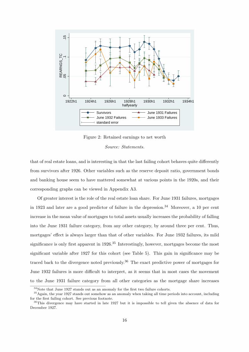
after 1926 for the third one. This is also illustrated in Figure 2, which is quite reminiscent of

31Interpretation of hazard ratios in the survival model is particularly tricky as most explanatory variables areratios, whose unit of analysis is unclear. As the following analysis will suggest, this obstacle can be overcome inmultinomial logistic modelling.

32As capital was seen to be either insignificant or to have inconsistent coefficients, it was dropped from theregression for increased degrees of freedom. This was also done for other real estate, borrowed funds and loanson collateral security, which are generally unimportant for the pre-depression period. Other controls seen to besometimes significant were kept in the regressions.

33Again, I make use of geometric means.

14

Table 4: Multinomial logistic model of bank failure: December 1924

Multinomial logit estimates Predicted marginal effectsJune 1931 June 1932 June 1933 June 1931 June 1932 June 1933

Reserve-deposit -3.517** -3.216** -2.982** -.001 -.019 -.007(1.38) (1.33) (1.25)

Gvt bonds -.067 -.156 -.071 .001 -.002 .000(.12) (.12) (.12)

Mortgages 1.958*** .436 -.166 .029 -.012 -.007(.64) (.40) (.47)

Other loans .708 .738 .082 .004 .006 -.003(.46) (.45) (.66)

Banking house .186 .091 .150 .002 -.001 .001(.08) (.06) (.09)

Retained earnings -1.329*** -.933 -.397 -.009 .003 .002(.39) (.37) (.47)

Const -3.220 -5.280 -6.608(3.05) (2.80) (4.00)

n = 95 Prob > chi2 = .012 Likelihood = -95.69

Notes: * significant at α = 0.01, ** significant at α = 0.05, *** significant at α = 0.10. The basecategory is Survivor. Standard errors in parentheses. Source: Statements.

Table 5: Multinomial logistic model of bank failure: June 1928


Reserve-deposit 1.258 -.043 -.883 .025 -.011 -.010(1.12) (1.04) (1.24)

Gvt bonds -.231 -.273 -.195 -.001 -.002 -.000(.21) (.21) (.22)

Mortgages 1.548*** .896** -.078 .020 .003 -.008(.48) (.40) (.35)

Other loans .886** .069 .295 .015 -.008 -.000(.34) (.21) (.44)

Banking house .229** .067 .067 .003 -.001 -.000(.35) (.36) (.37)

Retained earnings -.559 -.283 -.736* -.003 .003 -.005(.35) (.36) (.37)

Const 6.528 .572 -4.336(3.22) (2.97) (3.25)



15

0.0

5.1

.15

RE

AR

NG

S_T

C



Figure 2: Retained earnings to net worth

Source: Statements.

that of real estate loans, and is interesting in that the last failing cohort behaves quite differently

from survivors after 1926. Other variables such as the reserve deposit ratio, government bonds

and banking house seem to have mattered somewhat at various points in the 1920s, and their

corresponding graphs can be viewed in Appendix A3.

Of greater interest is the role of the real estate loan share. For June 1931 failures, mortgages

in 1923 and later are a good predictor of failure in the depression.34 Moreover, a 10 per cent

increase in the mean value of mortgages to total assets usually increases the probability of falling

into the June 1931 failure category, from any other category, by around three per cent. Thus,

mortgages’ effect is always larger than that of other variables. For June 1932 failures, its mild

significance is only first apparent in 1926.35 Interestingly, however, mortgages become the most

significant variable after 1927 for this cohort (see Table 5). This gain in significance may be

traced back to the divergence noted previously.36 The exact predictive power of mortgages for

June 1932 failures is more difficult to interpret, as it seems that in most cases the movement

to the June 1931 failure category from all other categories as the mortgage share increases

34Note that June 1927 stands out as an anomaly for the first two failure cohorts.35Again, the year 1927 stands out somehow as an anomaly when taking all time periods into account, including

for the first failing cohort. See previous footnote.36This divergence may have started in late 1927 but it is impossible to tell given the absence of data for

December 1927.

16

0.0

1.0

2.0

3.0

4O

TH

ER

_RE

_TA



Figure 3: Other real estate to total assets

Source: Statements.

dominates all other movements. Together these results are strong evidence that the amount of

mortgages held was a crucial factor in failure for two failure cohorts out of three.37

The variable “other real estate” from Table 3 deserves special attention. Other real estate is

an asset consisting of property repossessed by the bank in the face of real estate foreclosures. It

is usually recognized by bankers as an undesirable asset and held only to minimize loan losses.

This variable should then be one of those variables representing a backfire effect of real estate

investment in the 1920s if banks felt the need to foreclose. Figure 3 shows precisely this.38

4.2 Historical explanation

So how can mortgages have mattered this much in practice? An answer to this question can be

found in a number of contemporary sources focusing on the role played by commercial banks

37No clear conclusions can be drawn about the third cohort, except perhaps that retained earnings to net worthseems to be its most important predictor of failure.

38One might question the importance of this variable in explaining bank failures given the very low percentagesshown in Figure 3 which never go much beyond 3 per cent. However, banks may have failed because they faceddeposit losses while holding a high share of mortgages maturing at a considerably later date, without the qualityof these mortgages necessarily deteriorating (more on this below). More importantly, each cohort’s last datapoint represents its status at the last call before failure, and each call occurred only every six months. Thismeans that if many banks failed between April and June, which was the case for the first two failing cohorts, itis likely that much of their repossessed property would not have been recorded by December before this date.Foreclosure was a very lengthy process - it took 18 months on average in Illinois - , which increases the odds thatmany of the effects of foreclosure are not visible on this graph (Child, 1925; Hoppe, 1926; Johnson, 1923).

17

in the Chicago building boom. An article published in an August 1929 issue of the Chicago

Tribune entitled “Claim Illinois is Overloaded with Banks” worried that too many banks were

in operation for too small a number of people (Chicago Tribune, n.d.). According to James,

“[these banks’] soundness was intimately related to the building boom” (James, 1938, p. 953).

Indeed, while some early-founded banks took part in the mortgage lending surge, many of these

banks were established on the outlying regions of Chicago to respond to the expanding suburbs

of the time.

The boom itself was the result of circumstances created by World War I. On the one hand,

a near wartime embargo on building material and labour created a housing shortage which

realtors were all too eager to compensate for after the war (U.S. Congress, 1921). On the other

hand, the war led to a substantial boom in agricultural goods and land, which quickly gave way

to a deep recession in farming areas when the war came to an end. As a flourishing business

centre laying next to the vast but weakened agricultural lands of the Midwest, Chicago profited

from this situation perhaps more than any other city in the U.S.

The excitement that the progress in economic activity and the near-constant arrival of new

dwellers in search of higher wages brought to the city led to an extremely fast development

of credit, termed “financial elephantiasis” by James (ibid., p. 939). Eichengreen & Mitchener

(2003) stress the interaction between the structure of the financial sector and the business

boom. While the rapid growth of installment credit first started with nonbank institutions,39

very quickly many sorts of financial institutions ended up competing for consumers’ credit.

One of the consequences of this credit expansion in Chicago was a substantial building

boom, which may have been particularly strong in the Chicago area, although so far there has

been no major academic study on 1920s real estate activity at a disaggregated level for the

country as a whole.40 The Chicago real estate boom was excessive in the sense that it reflected

predictions of population increase that went far beyond the actual increase. Hoyt shows how

as Chicago’s population started growing at an unusually rapid rate investors imagined that a

“new era” was born and that Chicago would grow to 18 million by 1974 (Hoyt, 1933, p. 403).41

39For example, in 1919 General Motors established the General Motors Acceptance Corporation (GMAC) tofinance the development of its mass market in motor vehicles.

40White (2009) studies the question for the country as a whole but does not disaggregate into the variousregions and cities of the US. For journalistic accounts see Allen (1931) and Sakolski (1966).

41Hoyt humorously depicts “distinguished scholars”’ assessments of the situation, which were often quite sur-prising (Hoyt, 1933, p. 388).

18

-

2,000

4,000

6,000

8,000

10,000

12,000

14,000

16,000

18,000

20,000

19

15

19

16

19

17

19

18

19

19

19

20

19

21

19

22

19

23

19

24

19

25

19

26

19

27

19

28

19

29

19

30

19

31

19

32

19

33

Figure 4: Annual amount of new buildings in Chicago

Source: Hoyt (1933, p.475).

While from 1918 to 1926 the population of Chicago increased by 35 per cent the number of

lots subdivided in the Chicago Metropolitan Region increased by 3,000 per cent (ibid., p. 237).

In 1928, Ernest Fisher, associate professor of real estate at the University of Michigan, studied

real estate subdividing activity and found that “periods of intense subdividing activity almost

always force the ratio of lots to population considerably above the typical” (Fisher, 1928, p. 3).

His explanation was that “the only basis for decision is the position of the market at the time

the manufacturer [makes] his plans,” which leads to procyclicality. But a population slowdown

occurred in 1928, just before the start of the depression. Figure 4 shows that the Chicago

building boom reached a peak in 1925 and then receded abruptly.

The role that small state banks played in allowing this building boom to occur was a de-

terminant one. In December 1929, state banks made up 95.5 per cent of all banks in the city

(University of Illinois Bulletin, 1929). There were only 10 national banks; however these banks

were large. Indeed at the time they reported close to 40 per cent of the aggregate resources of

all banks (ibid.). The largest of these national banks, First National, rivaled in size the largest

bank in Chicago (Continental Illinois, which was state-chartered). As a contemporary made

clear, “by the summer of 1929, then, the Continental Illinois and the First National towered over

the Chicago money market like giants” (James, 1938, p. 952).42 Yet a huge number of small unit

banks swarmed around the city, most of them state-chartered. As James put it “around these

great banks of the Loop, there nestled, however, some 300 outlying commercial banks, each of

42Indeed, together they were responsible “for about half of the banking business transacted in the city” (ibid.).

19

which appeared microscopic with the Continental or the First although, in the aggregate, they

handled a considerable proportion of the city’s business.” Perhaps more importantly according

to James, “most were the outgrowths of the real estate boom” (ibid., p. 953). Indeed, Illinois

banking law facilitated the chartering of small unit banks to compete with national banks, and

thus contributed to the empowerment of relatively incompetent managerial staff whose interests

often coincided with those of property developers (see Appendix A4 for more detail).

4.3 Mortgage contracts

It has recently been suggested, not without reason, that the particular structure of commercial

bank mortgage lending characteristic of the 1920s (which changed radically in the 1930s) could

not have led to substantial trouble among mortgage borrowers and lenders. Specifically, three

of the major characteristics of these so-called “balloon” mortgages are often mentioned: the

short (on average of 3- to 5-year) maturity of these loans, a 50 per cent loan-to-value ratio, and

repayment of the principal at the end (Field, 2013; White, 2009).43 According to this view,

in the event of foreclosure even banks facing a catastrophic drop in house prices would have

quickly recovered the principal. Also implied in this account is the idea that if the peak in new

mortgage lending was reached around 1926, most of these loans would have been repaid by the

start of the depression. Figure 5 shows the increase in new mortgages in Cook county at the

time.

Yet an inquiry into the practice of mortgage refinancing suggests a different picture. In-

deed, precisely because these loans were relatively short-term (and perhaps for other reasons)

borrowers generally expected to be able to roll over these loans at maturity. As Saulnier made

clear in his 1956 study of 1920s mortgage lending in the US, “the much lauded feature of full

repayment by maturity has been won at the price of extended maturities” (see Morton (1956,

p. 8) and Chapman & Willis (1934, p. 602)). The precise average contract length for loans made

in 1926 was 3.6 years (for commercial banks), and 3.1, 2.5 and 3.2 years for loans made in 1925,

1927 and 1928 respectively (ibid., p. 174).44 For 1927 loans, maturity would be reached around

mid-1929, and for 1928 loans around mid-1931. In 1925 the amount of new mortgages in Cook

43Snowden (2010) also provides information on the structure of commercial bank mortgages in the 1920s.44Since these figures are based on National Bureau of Economic Research survey of urban mortgage lending,

their absolute precision may be taken with care. The survey was made in 1947 on a sample of 170 commercialbanks, “representing about one-third of the commercial banks total nonfarm mortgage portfolio as of mid-1945.”It included “commercial banks of all sizes” (ibid., p. 71).

20

0

500

1000

1500

2000

-

200,000,000

400,000,000

600,000,000

800,000,000

1,000,000,000

1,200,000,000

1920 1921 1922 1923 1924 1925 1926 1927 1928 1929 1930 1931

Figure 5: New mortgages and trust deeds, Cook County, Illinois ($)

Note: the source does not specify whether new mortgages include renewed mortgages. Source:Hoyt (1933, p.475).

County was slightly lower than in 1927, but taking this year into account would still mean that

a large portion of mortgages were expected to be refinanced in early 1929 (the average contract

length for 1925 loans was 3.1 years). Morton points out that even for mortgages made before

1924 inclusive (so likely unaffected by the depression), the realized maturity was in fact 7.5

years. For the 1925-29 period, the realised maturity was 8.8 years (ibid., p. 119). Evidence thus

shows that it is unlikely that most of these loans would have been repaid by 1929.

In this context it is interesting to quote from a document published by the Federal Home

Loan Banks in 1952 on the matter:

“Another thorn was the uncertainty and recurring crises in the credit arrange-ments inherent in the then prevalent practice of buying a home with a first mortgagewritten for one to five years, without any provision for paying back the principal ofthe loan during that time. This latter device was a fair weather system, and, as isthe case with most such systems, nobody suspected that there was anything wrongwith it until the weather changed.

What usually happened was that the average family went along, budgeting forthe interest payments on the mortgage, subconsciously regarding the mortgage itselfas written for an indefinite period, as if the lender were never going to want his moneyback This impression was strengthened by the fact that lenders most frequently didrenew the mortgage over and over again when money was plentiful” (Federal HomeLoan Bank Board, 1952, pp. 2-5).

As this excerpt shows, it is difficult to exclude the possibility that loans made in 1926-7

had at least some impact during the Great Depression. In particular, as banks faced large

21

withdrawals at the same time as many of these loans came to maturity (see next section), they

were more likely to refuse to renew them and demand repayment instead (Gries & Ford, 1932).

Should borrowers be unable to do so due to renewal expectations, banks would foreclose. In

this case they would theoretically be able to recover the principal on their first mortgage loans

whatever the fall in house prices, given the 50 per cent loan-to-value ratio. However, they in

fact had to wait for another 18 months on average before acquiring title to the property (Child,

1925; Hoppe, 1926; Johnson, 1923), which considerably increased the length of the liquidation

process, and thus made failure more likely (see also Federal Reserve Committee on Branch,

Group and Chain Banking (1939)).45

There are unfortunately no good statistics on the rate of foreclosure for commercial banks

in Chicago. Most of the numbers are provided by Hoyt (1933, p. 269-270), and they concern the

total amount of foreclosures: “Foreclosures were mounting rapidly, the number increasing from

5,818 in 1930 to 10,075 in 1931, [and] reached a new peak in 1932, rising to15,201.” While it is

thus not possible to describe banks’ precise losses in real estate, it is still worth investigating the

links between their mortgage shares and deposit losses as determinants of bank failure, which

is the topic of the next section.

5 The Liquidity Shock: Analysis of Bank Liabilities

This section examines the interactions between mortgages as a determinant of failure and the

liability side of the balance sheet (in particular, deposit losses). Key variables used in this

section are the cumulative rates of decline in deposits from June 1929 to December 1930 (just

before the first failure cohort drops out), from June 1929 to December 1931 (just before the

second failure cohort drops out), and from June 1929 to December 1932 (just before the third

one drops out). Note that the data on deposits come from the last call before failure, which for

some failures was almost six months before their failure date. As both 1931 and 1932 panics

occurred in April and/or June, this means that on average, for banks that failed during panics,

45Note that the question of alleged safety due to the 50 per cent down payment was not tackled here. Thisissue is in part the focus of another paper, in which I show that in a majority of cases commercial bank borrowerscould not in fact make such a high down payment, but only paid down 25 per cent, borrowing the rest in theform of a second, junior mortgage at an exorbitant interest rate (around 14 per cent). This also reduced thelikelihood of repayment of the first mortgage. Indeed, the second mortgage system was a major flaw of the 1920smortgage structure (see Postel-Vinay (2013b)).

22

−.8

−.6

−.4

−.2

0.2

DE

PC

GR

OW

TH

1924

h2

1925

h1

1925

h2

1926

h1

1926

h2

1927

h1

1927

h2

1928

h1

1928

h2

1929

h1

1929

h2

1930

h1

1930

h2

1931

h1

1931

h2

1932

h1

1932

h2

halfyearly


Figure 6: Mean cumulative growth rate of total deposits (base time: June 1929)

Source: Statements.

these variables do not reflect their losses at the last panic before failure.46

The first thing to note is that all banks lost tremendous amounts of deposits. In 1930 the

first failure cohort lost on average 22 per cent of deposits, and from 1930 to 1931 the second,

third and survivor cohorts lost respectively 59 per cent, 43 per cent and 37 per cent. Figure

6 shows the cumulative growth rate of total deposits, and Table 6 shows each cohort mean

as well as tests of differences between them. In such circumstances it would be expected that

banks with the highest amounts of illiquid assets (mortgages in most cases) would not be able

to liquidate their assets fast enough to cover the deposit losses and would thus fail.

To what extent was the shock to liabilities endogenous to the share of mortgages? While

this question is difficult to answer certain pieces of evidence can help to draw a few preliminary

conclusions. Table 7 provides results of an OLS model with deposit losses as the dependent

variable and the usual ex ante variables on the right-hand side. From this model it appears that

for June 1931 failures none of the fundamental variables explain their deposit losses between

June 1929 and December 1930, thus suggesting that withdrawals from these banks were on

average not information-based, despite an absence of significant panics in this period (Wicker,

46A survival model for the liability side is available in Appendix B3. It confirms the importance of depositlosses in predicting failure, while rejecting any significant role for capital.

23

Table 6: Tests of differences between mean deposit growth rates

Survivors June 1931 June 1932 June 1933(1) (2) (3) (1) (1) (2) (1) (2) (3)

Mean -.08 -.37 -.59 -.22 -.17 -.59 -.00 -.43 -.63(.07) (.06) (.08) (.04) (.03) (.03) (.13) (.10) (.09)

June 1931(t-stat)

1.806*

June 1932(t-stat)

1.298 3.380*** -.995

June 1933(t-stat)

-.527 .472 .366 -1.606 -1.288 -1.550

Observations 35 46 36 14

Notes: * significant at α = 0.01, ** significant at α = 0.05, *** significant at α = 0.10.(1) June 1929 - Dec 1930 cumulative deposit losses;(2) June 1929 - Dec 1931 cumulative deposit losses;(3) June 1929 - Dec 1932 cumulative deposit losses.First row gives the mean deposit growth rates (standard errors in parentheses). Next rows give t-statistics of differences between two means. Source: Statements.

Table 7: OLS Results (dependent variable: deposit losses)

June 1931 F.and Survivors

June 1932 Failuresand Survivors

June 1933 Failures and Survivors

Variable in June 1929 (1) (1) (2) (1) (2) (3)

Cash reserves to totalassets

-.032 .029 .096 .053 .308 .222(.14) (.19) (.24) (.27) (.25) (.40)

Gvt bonds .008 .002 .018 .009 .013 -.011(.01) (.01) (.01) (.02) (.02) (.02)

Mortgages -.074 -.074 -.151*** -.063 -.113* -.065(.05) (.05) (.05) (.06) (.07) (.05)

Other loans -.044 -.012 .011 -.057 -.005 -.096(.04) (.04) (.05) (.06) (.06) (.09)

Banking house .004 -.000 -.015* -.001 -.002* -.014(.01) (.01) (.01) (.01) (.01) (.02)

Retained earnings .081 .015 .089 .013 .070 .190*(.05) (.04) (.07) (.04) (.06) (.10)

Const -.190 -.167 -.514 -.173 -.043 -.588(.37) (.50) (.57) (.68) (.61) (.99)

n 75 66 66 45 45 45R2 .11 .09 .31 .08 .34 .17Prob > F .101 .111 .106 .416 .378 .091

Notes: * significant at α = 0.01, ** significant at α = 0.05, *** significant at α = 0.10. Standard errorsin parentheses. The explanatory variables are taken in June 1929. Source: Statements.(1) June 1929 - Dec 1930 cumulative deposit losses;(2) June 1929 - Dec 1931 cumulative deposit losses;(3) June 1929 - Dec 1932 cumulative deposit losses.

24

1996).47 This is confirmed by the figures on deposit losses provided above in Table 6 where it

appears that the difference in deposit losses between this first failure cohort and survivors is

only borderline significant, and is not significant when comparing to other failure cohorts. On

the other hand, for the second failure cohort, mortgages predict 1931 deposit losses well (though

the R-squared is relatively low), a result consistent with the fact that the magnitude of their

withdrawals significantly differed from survivors’.48 Yet even in this case deposit losses were

very large for survivors (around 37 per cent compared to 59 per cent for June 1932 failures).

Together these results suggest that while mortgages remain essential to explain Chicago bank

failures, the role of mass, non-discriminating deposit withdrawals cannot be disregarded.

Now the causes of these indiscriminate withdrawals in the preceding non-panic windows are

open to debate. Tentative answers may be found in the literature on bank runs. According

to Diamond & Dybvig (1983), bank runs are undesirable equilibria in which borrowers observe

random shocks (sunspots) and withdraw their deposits, thus causing even “healthy” banks to

fail. Others, such as Calomiris & Gorton (1991) and Calomiris & Kahn (1991), have stressed the

role of signal extraction in the context of asymmetric information between depositors and bank

managers. In this view, depositors observe a specific shock to banks’ assets, but do not know

which banks have been most hit. They therefore run on all banks, which causes only the weaker

banks to fail. Bank runs thus act as a form of monitoring: unable to costlessly value banks’

assets, borrowers use runs to reveal the unhealthy banks. This paper argues that indiscriminate

withdrawals revealed the banks with the most illiquid assets, which partly supports this view.

But whether depositors observed a particular shock or not remains to be determined.

So did banks fail in the first and second episodes simply because they had a particularly large

share of mortgages, or because of the particularly low quality (in terms of underlying values)

of these mortgages? Again, while quality may have mattered, mortgages’ sheer lack of liquidity

posed a tremendous challenge to banks. Figure 1 showed how real estate loans increased as a

share of total assets for all banks during the depression, at the same time as assets as a whole

were diminishing.49 Other types of loans, on the other hand, were promptly liquidated in this

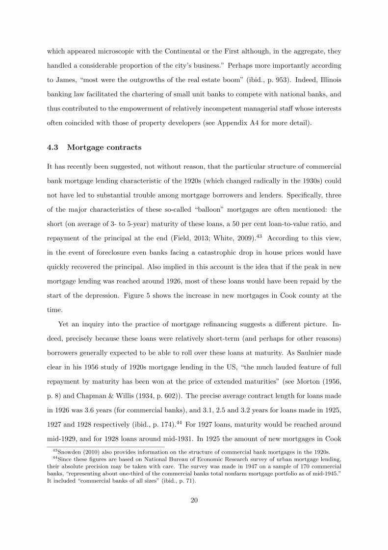
period. Figure 7 shows the falling share of loans on collateral security owned by banks, while

47Note that bank statements were released to the public every six months by the State Auditor.48Note that these figures differ slightly from Calomiris & Mason (1997)’s as their sample included national

banks as well. Their survivor category also includes my June 1933 Failures cohort.49For a graph of total assets see Figure 14 in Appendix B1.

25

.1.2

.3.4

SE

CLO

AN

S_T

A



Figure 7: Loans on collateral security to total assets

Source: Statements.

0.0

5.1

.15

.2.2

5O

TH

LOA

NS

_TA



Figure 8: Other loans to total assets

Source: Statements.

26

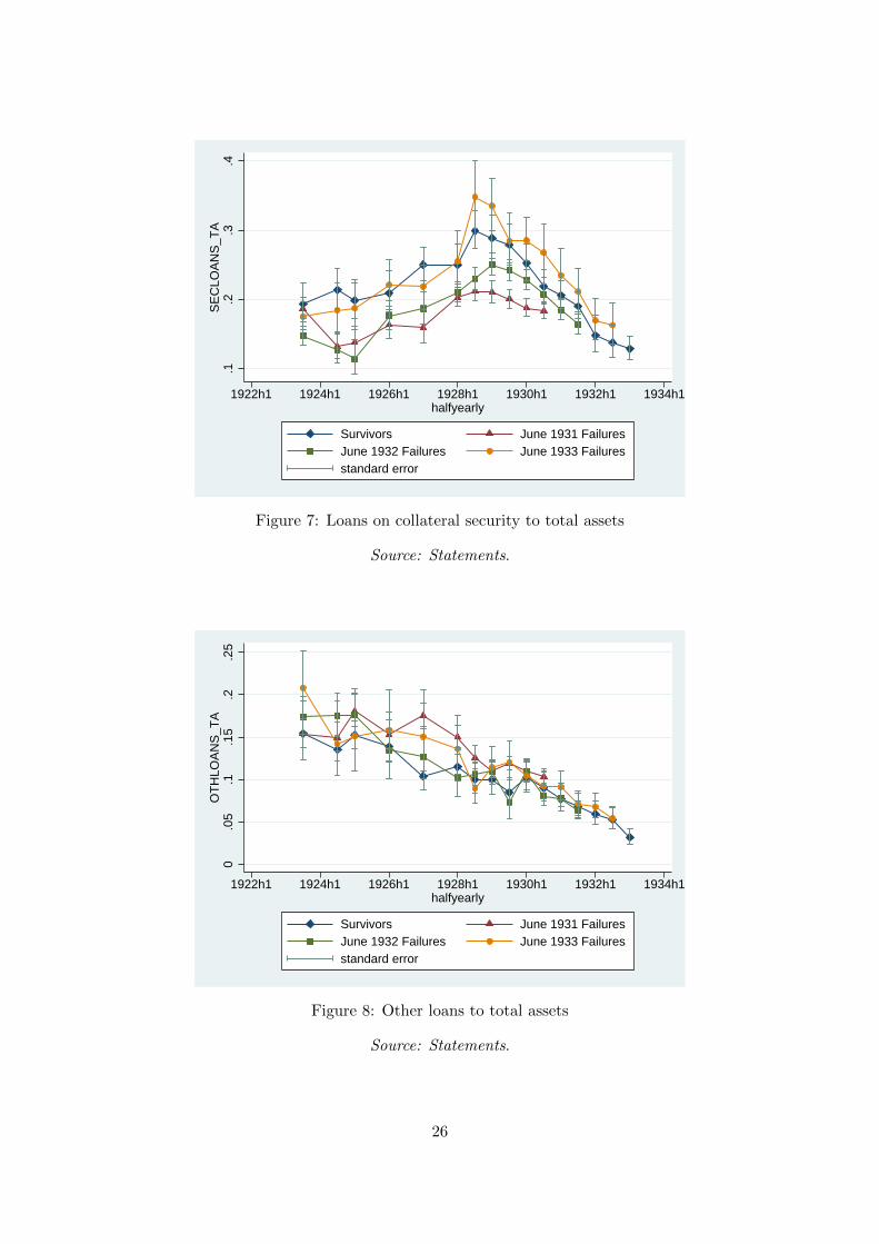
Figure 8 shows a similar decline in other loans as a share of total assets. Compared to other

assets, therefore, mortgages were notoriously difficult to liquidate. As all banks engaged in fire

sales they became the main constraint on their liquidation process.50

These results therefore shed new light on the current debate about the nature of the causes

of bank failures during the Great Depression. On the one hand, some have emphasised the

importance of massive and non-discriminatory bank runs which caused even solvent banks

to fail (Friedman & Schwartz, 1963). On the other hand, many have insisted that banks

suffered fundamental troubles beforehand, and that insolvent banks were the most likely to

fail even during asymmetric-information panics (Calomiris & Mason, 1997, 2003; White, 1984).

In particular, Calomiris & Mason (1997) have shown that Chicago banks failing during the

June 1932 panic had in fact lost a higher amount of deposits in 1931, thereby indicating that

depositors identified beforehand which banks were potentially insolvent, and that the differential

in cumulative deposit losses may have been important in explaining actual failure.

While confirming Calomiris and Mason’s (1997) findings regarding the importance of banks’

fundamentals prior to failure, and insisting on the importance of mortgages in particular, the

results on deposit losses for all three cohorts suggest a slightly different picture. Indeed, it

appears that the origin of Chicago banks failure can be found in a combination of impaired

fundamentals on the one hand, and a general run on deposits on the other.

6 Conclusion

Looking into the long-term behaviour of Chicago banks in the 1920s yielded new insights into the

causes of their failure. I showed that for two cohorts out of three, banks’ long-term investments

in illiquid assets (especially mortgages) severely weakened their position when they came to

face largely indiscriminate runs on their deposits. Though restricted to Chicago, these results

reassert the role that liquidity issues played in the Great Depression, both on the liability and

50Security loans were mainly call loans, that is, loans repayable at the option of the lender within twenty-four hours’ notice. Funds were lent in this way to individuals who used them to carry securities, for examplewhen dealing with them on margin. The securities themselves were used as collateral for these loans, with theunderstanding that they were likely to be withdrawn at any time. According to Bogen & Willis (1929, p. 245),“depositors can, and sometimes do, determine the calling of loans by the activity of their own demands.” Otherloans were short-term commercial loans, often sought by companies for the seasonal expansion of their inventories.In such cases “the customer of the commercial bank is expected to pay off or “clean up” his obligations to it atcertain intervals” (ibid., p. 11). Both types of loans were eligible for rediscount at the Federal Reserve Banks orcould be sold in the open market, while mortgages in general were not (Bogen & Willis, 1929; U.S. Congress,1927).

27

the asset sides of the balance sheet. An important task for future research will be to assign

specific responsibilities to the sheer size of long-term, non-marketable assets on the one hand,

and to their quality on the other. For this aim to be achieved, the search for more detailed

asset data needs to be continued.

This paper also reassessed the role that mortgage investments played in the Great Depression

via the banking channel. Parallels with the recession starting in 2007 may be tentatively drawn,

though differences in mortgage structure between now and then are noteworthy. In the 1920s,

mortgage securitization by Chicago commercial banks was limited, and certainly not nationwide

in scope.51 This created problems as real estate loans were not eligible for rediscount at the

Federal Reserve Banks. Banks investing in real estate were therefore particularly vulnerable

to liquidity shocks, and given the long-term liquidation process mortgages required, temporary

help from the Federal Reserve may not have been sufficient to alleviate the situation (thus

questioning Friedman & Schwartz (1963)’s policy recommendations).52

Yet there is an important similarity between the two crises. In both cases banks suffered

tremendous liquidity shocks on the liability side of their balance sheets, which, regardless of

their origin, highlighted the intrinsically illiquid character of mortgages in the presence of under-

developed or inefficient securitization. In the 1920s, banks suffered large deposit withdrawals,

and those who had heavily engaged in mortgage investments failed. In the late 2000s, the

uninsured repo market collapsed (Gorton & Metrick, 2012), and all buyers and sellers of real

estate securities became exposed to its fallout. This arguably contributed to the failure of large

banking institutions. Thus, while institutions were quite different now and then, the effects of

the liquidity shocks on bank failure via their mortgage portfolio were similar.

Finally, important differences in the geographical pattern of bank failures should be noted.

During the Great Depression, while a large number of banks failed in the northeastern cities

of the U.S., many of which presented similar characteristics to Chicago, just as many banks

failed in the vast agricultural areas of the Midwest and the South. We know that banks had

been failing in these areas for most of the 1920s due to the post-war farming crisis (which also

translated into a deep agricultural land crisis) but what we still do not know is how, starting

in 1930, the largest banking crisis in history came about, first in these agricultural lands, and

51see Postel-Vinay (2013a).52Another difference is that by the late 2000s the quality of mortgages was impaired, which in the 1920s case

remains to be proven.

28

then in the cities. The only common cause is World War I, but the timing of this peculiar kind

of twin crisis is poorly understood at present.

29

References

F. L. Allen (1931). Only Yesterday: An Informal History of the Nineteen-Twenties. Harperand Brothers, New York.

Board of Governors of the Federal Reserve System (1937). Federal Reserve Bulletin. FederalReserve System.

J. I. Bogen & H. P. Willis (1929). Investment Banking. Harper & Brothers, New York.

C. W. Calomiris & G. Gorton (1991). ‘The Origins of Banking Panics: Models, Facts, andBank Regulation’. In R. G. Hubbard (ed.), Financial Markets and Financial Crises. TheUniversity of Chicago Press.

C. W. Calomiris & C. M. Kahn (1991). ‘The Role of Demandable Debt in Structuring OptimalBanking Arrangements’. The American Economic Review 81(3).

C. W. Calomiris & J. R. Mason (1997). ‘Contagion and Bank Failures During the GreatDepression: the June 1932 Chicago Banking Panic’. American Economic Review 87(5).

C. W. Calomiris & J. R. Mason (2003). ‘Fundamentals, Panics, and Bank Distress During theDepression’. American Economic Review 87(5).

C. W. Calomiris & D. C. Wheelock (1995). ‘The Failures of Large Southern Banks During theGreat Depression’. Columbia University Working Paper .

M. Carlson (2001). ‘Are Branch Banks Better Survivors? Evidence from the Depression Era’.Federal Reserve Board Working Paper 2001(51).

S. B. Carter, et al. (2006). Historical Statistics of the United States. Cambridge UniversityPress, Cambridge.

J. M. Chapman & H. P. Willis (1934). The Banking Situation, American Post-War Problemsand Developments. Columbia University Press, New York.

Chicago Tribune (n.d.). Various issues. Chicago Tribune, Chicago, Ill.

S. R. Child (1925). ‘A Uniform Mortgage Law for All the States’. Real Estate Finance .

D. W. Diamond & P. H. Dybvig (1983). ‘Bank Runs, Deposit Insurance, and Liquidity’. Journalof Political Economy 91(3).

B. Eichengreen & K. Mitchener (2003). ‘The Great Depression as Credit Boom Gone Wrong’.BIS Working Paper 137.

M. Esbitt (1986). ‘Bank Portfolios and Bank Failures During the Great Depression: Chicago’.Journal of Economic History 46(2).

Federal Home Loan Bank Board (1952). The Federal Home Loan Bank System, 1932-195.Federal Home Loan Banks, Washington, D. C.

Federal Reserve Committee on Branch, Group and Chain Banking (1939). 225 Bank Suspen-sions, Case Histories From Examiners’ Reports. Federal Reserve System, Washington, D.C.

30

A. J. Field (2013). ‘The Interwar Housing Cycle in the Light of 2001-2011: A ComparativeHistorical Approach’. NBER Working Paper 18796.

E. M. Fisher (1928). ‘Real Estate Subdividing Activity and Population Growth in Nine UrbanAreas’. Michigan Business Studies 1(9).

M. Friedman & A. J. Schwartz (1963). A Monetary History of the United States, 1867-1960.Princeton University Press, Princeton.

C. M. Gambs (1977). ‘Bank Failures - An Historical Perspective’. Monthly Review FederalReserve Bank of Kansas City 62.

W. N. Goetzmann & F. Newman (2010). ‘Securitization in the 1920’s’. NBER Working Paper15650.

G. Gorton & A. Metrick (2012). ‘Securitized Banking and the Run on Repo’. Journal ofFinancial Economics 104:425.

J. M. Gries & J. Ford (1932). The Presidents Conference on Home Building and Home Own-ership, called by President Hoover, Home Finance and Taxation. National Capital Press,Washington, D. C.

M. Guglielmo (1998). Illinois State Bank Failures in the Great Depression. Ph.D. thesis,University of Chicago.

W. J. Hoppe (1926). ‘Assignment of Rents as Additional Security for Second Mortgages’. RealEstate Finance .

H. Hoyt (1933). One Hundred Years of Land Values in Chicago, The Relationship of theGrowth of Chicago to the Rise in its Land Values, 1830-1933. The University of ChicagoPress, Chicago.

Illinois Auditor of Public Accounts (n.d.). Statement Showing Total Resources and Liabilitiesof Illinois State Banks. Journal Printing Company, Springfield. Various years.

F. C. James (1938). The Growth of Chicago Banks. Harper and Brothers Publishers, New York.

F. L. Johnson (1923). ‘How Banks and Mortgage Companies Can Help the Realtor’. Real EstateFinance .

B. Lev & S. Sunder (1979). ‘Methodological Issues in the Use of Financial Ratios’. Journal ofAccounting and Economics 1:187.

J. R. Mason (1998). ‘American Banks During the Great Depression: A New Research Agenda’.Federal Reserve Bank of St Louis Review 80(3).

J. B. McFerrin (1939). Caldwell and Company: A Southern Financial Empire. Chapel Hill.

S. Mcleay & D. Trigueiros (2002). ‘Proportionate Growth and the Theoretical of FinancialRatios’. Abacus 38(3).

R. McNally (n.d.). Rand McNally Bankers Directory. Rand McNally and Co., New York.Various years.

T. Messer-Kruse (2004). Banksters, Bosses and Smart Money: A Social History of the ToledoBank Crash of 1931. Ohio State University Press, Columbus.

31

K. J. Mitchener (2005). ‘Bank Supervision, Regulation, and Instability during the Great De-pression’. Journal of Economic History 65(1).

J. E. Morton (1956). Urban Mortgage Lending: Comparative Markets and Experience. PrincetonUniversity Press, Princeton.

N. Postel-Vinay (2013a). ‘Chicago Banks’ Mortgage Securitization in the Great Depression’.Working paper.

N. Postel-Vinay (2013b). ‘The Evils of Ultraconservative Lending. U.S. Commercial BankMortgages from 1913 to the Great Depression’. Working paper.

G. Richardson (2007). ‘Categories and Causes of Bank Distress During the Great Depression,1929-1933: the Illiquidity versus Insolvency Debate Revisited’. Explorations in EconomicHistory 44:588.

R. G. Rodkey (1935). ‘State Bank Failures in Michigan’. Michigan Business Studies 7(2).

R. G. Rodkey (1944). Sound Policies for Bank Management, A Discussion for Bank Officersand Directors. The Ronald Press Company, New York.

A. M. Sakolski (1966). The Great American Land Bubble: The Amazing Story of Land-Grabbing,Speculations, and Booms from Colonial Days to the Present Time. Johnson Reprint Corp,New York.

K. Snowden (2010). ‘The Anatomy of a Residential Mortgage Crisis: A Look Back to the 1930s’.NBER Working Paper 16244.

R. Thomas (1935). ‘Bank Failures Causes and Remedies’. Journal of Business of the Universityof Chicago 8(3).

M. Tippett (1990). ‘An Induced Theory of Financial Ratios’. Accounting and Business Research21(81).

University of Illinois Bulletin (1929). ‘An Analysis of Earning Assets of Chicago Banks’.

U.S. Congress (1921). Hearings before the Select Committee on Reconstruction and Production,United States Senate, Sixty-Sixth Congress, Third Session, pursuant to S. Res. 350, Autho-rizing the Appointment of a Committee to Inquire into the General Building Situation and toReport to the Senate before December 1, 1920, such Measures as may be Deemed Necessaryto Stimulate and Foster the Development of Construction Work in all its forms. GovernmentPrinting Office.

U.S. Congress (1927). ‘Hearings before the Committee on Banking and Currency, House of Rep-resentatives, Sixty-Ninth Congress, First Session on H.R. 7895, A Bill to Amend Paragraph(d) of Section 14 of the Federal Reserve Act, as Amended, to Provide for the Stabilization ofthe Price Level for Commodities in General.’.

D. Van Hoose (2010). The Industrial Organization of Banking, Bank Behavior, Market Structureand Regulation. Springer, Berlin.

R. B. Vickers (2011). Panic in the Loop: Chicago’s Banking Crisis of 1932. Lexington Books,Plymouth.

32

E. N. White (1984). ‘A Reinterpretation of the Banking Crisis of 1930’. Journal of EconomicHistory 44(1).

E. N. White (2009). ‘Lessons from the Great American Real Estate Boom and Bust of the1920s’. NBER Working Paper 15573.

E. Wicker (1996). The Banking Panics of the Great Depression. Cambridge University Press,Cambridge.

33

A Reader Appendix

A.1 Sources, name changes and consolidations

This study uses the Statements of State Banks of Illinois. The Reports of Condition from the

Office of the Comptroller of Currency focus on all member banks (both state and national)

nationwide at disaggregated levels, and contain very detailed information on individual banks,

including qualitative information. For my study these reports would have proved insufficient:

the extant reports for state member banks are available for the same dates as the Statements

and are less complete since they include only state member banks, and for national member

banks the only available reports are for December 1929 and December 1931.53 There are no

reports for 1930, which is a crucial year for this research. Focusing on state banks should not be

a problem since as pointed out before, state banks accounted for 87.6 percent of all suspensions,

whereas national banks accounted for only 12.4 per cent of suspensions (White, 1984).

Creating cohorts is an essential way of keeping track of the same sample of banks, whether

failures or survivors (aside from its advantages for economic analysis). Another essential feature

of this aim is linked to name changes and consolidations. As previously mentioned, I had all the

data needed for this purpose. Name changes were corrected in 26 instances. However, I still had

to make decisions about whether to include a merger or acquisition in the failing or surviving

categories. Most authors include such consolidations as failures; that is, a bank that was taken

over is usually considered a failure, and so are both of the banks that merged, even when the

merger itself ended up surviving the depression. For instance, Calomiris & Mason (2003) specify

that their data “contain almost seventy different ways a bank can exit the dataset, ranging from

all imaginable types of mergers and acquisitions to relatively simple voluntary liquidations and

receiverships; [...] together, we term [them] failures.” The Reports of Condition they used were

more detailed in this respect, and I do not have data on all types of mergers and acquisitions.

Nevertheless, the Rand McNally directory gives sufficient detail at least on whether a merger

or a simple takeover occurred.

As in Calomiris & Mason (2003) I thought reasonable to count as failures banks that were

taken over by other banks. This occurred in 14 cases since June 1929. The banks that were

taken over before June 1929 are not taken into account in the sense that only the resulting

53Details of the available volumes are described in Mason (1998).

34

Table 8: State mergers between June 1929 and June 1933

Bank 1 Bank 2 New merger Firstreporting

date

Failing?

The ForemanTrust and

Savings Bank

State Bank Foreman-StateTrust and

Savings Bank

Dec 1929 Yes, June1931

Roosevelt StateBank

Bankers StateBank

Roosevelt-Bankers State

Bank

June 1930 Yes, Aug1930

Builders andMerchants State

Bank

Capital StateSavings Bank

Builders andMerchants Bank

and Trust Co

Nov 1930 Yes, April1931

Central Trust Coof Illinois

Chicago Trust Co Central RepublicBank and Trust

Co

July 1931 No

Sources: Statements, and Rand Mc Nally Bankers’ Directory.

consolidation should be part of a cohort. Exactly the same applies to pre-June 1929 mergers:

only the resulting merger can be part of a cohort and thus only this bank will be tracked down

as early as possible in the 1920s. Table 8 shows the state mergers that occurred since June 1929

and whether the merger ended up failing or not.

For the mergers that had failed by June 1933, there is no apparent dilemma regarding how

to classify the original consolidating banks. That is, when a merger ended up failing, the two

original banks’ data could be kept until they merge under a new name, at which point the

new merger’s data could be excluded from the dataset, making the two original banks failures

at the time of consolidation. Yet this decision sounds slightly arbitrary given the fact that a

healthy bank may have merged with a less healthy bank which may have dragged the former

into bankruptcy. In the first and third cases shown in Table 8, it was actually possible to divide

the merger’s balance sheet in two proportional parts and make the two original banks continue

until the time the merger itself fails. In the second case, the merger itself fails in August 1930

so could not be part of any cohort. Results are robust to different categorisations.

In the dataset only one state merger actually survived in Chicago: the Central Republic

Bank and Trust Co, a July 1931 consolidation of Central Trust Co of Illinois, Chicago Trust

Co and a national bank, the National Bank of the Republic. As in the previous cases, it was

decided that both state banks would be kept “alive” by taking the items on the balance sheet

of the new merger and splitting them into parts proportional to each original banks share of

35

the total.54

Finally, it seems necessary to specifically discuss the case of the Continental Illinois Bank

and Trust Company, which was the largest bank in Chicago in 1929, and which with the First

National Bank (as its name indicates, a national bank) “towered over the Chicago money market

like giants” (James, 1938, p. 952). Together they were responsible for about half of the business

transacted in the city (ibid.). Initially this bank was not included in the sample, for the simple

reason that it apparently failed in December 1932 and thus could not be part of a particular

cohort. However, it was soon discovered that the “failure” of the bank was in fact due to a rare

phenomenon at the time: the fact that it adopted a national charter. The Chicago Tribune

titled in October 1932 “CONTINENTAL GETS NATIONAL BANK CHARTER” which was

at the time seen as a strange kind of event (Chicago Tribune, 1932). One of the reasons this

happened, as the article explained, is that national banking laws were in the process of being

changed to allow branching everywhere, including in states that technically forbade it. As the

crisis made clear to some bank managers the potential benefits of branching, it is not surprising

that a strong bank like Continental Illinois sought after a national charter, and was granted

one.55 The bank was thus manually categorised as a survivor.

A.2 Additional multinomial logistic results

Tables 9, 10 , 11 , 12, 13, and 14 show multinomial logit results for December 1923, June 1925,

June 1926, June 1927, December 1928 and June 1929.

54But again the results are robust either way. See footnote above in section three on the controversial aspectof this rescue. I also thank Joseph Mason for kindly making national bank data available to me.

55The adjective “strong” here is based on the fact that Continental Illinois in June 1929 had healthier ratiosthan even the average of survivors. I do not know of any other state banks in Chicago which adopted a nationalcharter at that time.

36

Table 9: Multinomial logistic model of bank failure: December 1923


Reserve-deposit -2.037 -2.311 -2.411 -.007 -.019 -.001(1.89) (1.84) (1.94)

Gvt bonds -.135 -.236** -.130 .000 -.003 .000(.12) (.10) (.20)

Mortgages 1.983*** .560 .272 .028 -.008 -.005(.72) (.50) (.82)

Other loans -.034 .225 .640 -.004 .003 .004(.33) (.35) (.73)

Banking house .258* .163** .457 .002 -.000 .002(.15) (.07) (.30)

Retained earnings -.217 -.059 .067 -.003 .001 .001(.35) (.33) (.67)

Const .816 -2.229 -1.609(4.08) (4.13) (4.68)





Reserve-deposit -1.635* -1.408 -1.190 -.013 -.001 -.002(.93) (.86) (.89)

Gvt bonds -.010 -.166* -.085 .002 -.003 -.000(.10) (.09) (.11)

Mortgages 1.240** -.017 -.012 .022 -.011 -.003(.52) (.34) (.42)

Other loans .784* .353 -.077 .010 -.000 -.003(.47) (.43) (.76)

Banking house .141 .028 -.004 .002 -.001 -.000(.09) (.05) (.09)

Retained earnings -1.091*** -.888** -.202 -.006 .003 .002(.36) (.36) (.36)

Const -.882 -4.525 -4.330(2.45) (2.23) (3.41)



37



Reserve-deposit -1.851 -1.402 -1.242 -.015 -.008 -.002(1.00) (1.00) (1.01)

Gvt bonds -.163 -.201 .022 -.001 -.002 .001(.14) (.14) (.15)

Mortgages 2.171*** .682* -.156 .031 -.007 -.006(.37) (.37) (.31)

Other loans .394* .087 .312 .005 -.003 .001(.24) (.24) (.63)

Banking house .157 .023 .086 .002 -.001 .000(.06) (.06) (.12)

Retained earnings -1.084** -.518 -.201 -.011 .005 .001(.46) (.41) (.52)

Const -.764 -2.758 -3.308(2.77) (2.44) (3.38)





Reserve-deposit -.013 -.674 -.764 .011 -.010 -.004(1.65) (.50) (.68)

Gvt bonds -.169 -.216 -.175 -.000 -.002 -.000(.14) (.14) (.16)

Mortgages 1.131** .340 -.057 .017 -.003 -.005(.54) (.30) (.40)

Other loans 1.119*** .121 .421 .001 -.000 .000(.33) (.26) (.57)

Banking house .168** .069 .089 .002 -.005 .000(-.43) (.40) (.54)

Retained earnings -.926** -.283 -.676 -.010 .006 -.000(.43) (.40) (.54)

Const 2.736 -1.259 -3.444(3.94) (1.93) (2.70)



38

Table 13: Multinomial logistic model: December 1928


Reserve-deposit 1.171 -.531 -2.573 .031 -.015 -.018(1.60) (1.28) (1.72)

Gvt bonds -.164 -.179* -.183 -.000 -.001 -.001(.11) (.11) (.11)

Mortgages 1.823*** .880** .185 .022 .001 -.006(.61) (.40) (.38)

Other loans 1.239*** .262 -.092 .019 -.008 -.004(.43) (.37) (.47)

Banking house .193** .060 -.040 .003 -.001 -.001(.09) (.06) (.07)

Retained earnings -.537* -.500 -.862** -.003 -.001 -.001(.31) (.32) (.44)

Const 7.670 .103 -8.585(3.73) (2.90) (4.39)



Table 14: Multinomial logistic model: June 1929


Reserve-deposit -1.100 -1.483* -1.358 -.001 -.012 -.004(.91) (.79) (.85)

Gvt bonds -.144 -.167* -.120 -.001 -.001 -.000(.10) (.09) (.09)

Mortgages 1.689*** .776** .374 .023 -.003 -.004(.50) (.37) (.27)

Other loans .716* .341 .317 .008 -.002 -.000(.37) (.32) (.46)

Banking house .172* .054 -.062 .003 -.000 -.001(.09) (.34) (.40)

Retained earnings -.523 -.369 -.935** .000 .003 -.009(.34) (.34) (.40)

Const 2.044 -1.660 -5.157(2.65) (2.31) (2.97)



39

A.3 Additional financial ratios

Figures 9, 10, 11 , 12 and 13 show the reserve-deposit ratio, U.S. government bonds to total

bonds and stocks, banking house to total assets, borrowed funds to total assets and capital to

total assets. Note that bills payable and rediscounts are a form of long-term, high interest debt,

which is in fact a good indicator of bank trouble. This is due to the fact that when deposits

are withdrawn from risky banks, they are forced to rely on high-cost, borrowed debt (Calomiris

& Mason, 1997). Figure 12 thus shows banks’ race for liquidity as they started losing deposits,

and a similar ordering as before is noticeable. As a side note, the June 1932 spike for survivors

and late failures may be due to a Reconstruction Finance Corporation (RFC) plan to inject

liquidity in banks that it deemed sound during the June 1932 crisis (Calomiris & Mason, 1997).

.1.2

.3.4

.5R

D1



Figure 9: Cash reserves to total deposits (includes cash, other cash resources, due from otherbanks)

Source: Statements.

40

0.1

.2.3

.4pg

vtbd

s_tb

ds



Figure 10: U.S. government bonds to total bonds and stocks

Source: Statements.

0.0

2.0

4.0

6.0

8.1

BA

NK

HO

US

E_T

A



Figure 11: Banking house, furniture and fixtures to total assets

Source: Statements.

41

0.1

.2.3

EX

DE

BT

_TA



Figure 12: Bills payable and rediscounts to total assets

Source: Statements.

.1.2

.3.4

CA

P_T

A



Figure 13: Capital to total assets

Source: Statements.

42

A.4 Problems with unit banking

In the 1920s all Chicago state banks operated under the unit banking system; they were not

allowed to open branches as Illinois banking law forbade it. Problems linked to unit banking

were numerous. The main reason branch banking is usually thought of as an advantage is that it

increases portfolio diversification. Branch banking can be contrasted to group or chain-banking

as branches of the same bank can pool their assets and liabilities together. When there is a

liquidity shortage at one of the banks in a chain, other member banks cannot simply transfer

funds to that bank for help, a problem which does not even arise in the branch banking system.

This may partly explain the collapse of the Bain chain in June 1931 which triggered the banking

crisis at that time (James, 1938, p. 994).

Yet the lack of portfolio diversification was not necessarily directly due to the unit banking

system. Indeed, Rodkey points to the fact that many small bankers prior to the depression felt

a moral duty to “meet all demands for good local loans” (Rodkey, 1944, p. 4). It also seems

that the lack of portfolio diversification was not the only disadvantage of unit banking. Rodkey

blamed this system for fostering the incompetence of bank managers:

“This system leads naturally to a multiplicity of small banks under local control,owned locally, and operated usually by citizens of the home community who mayor may not have some knowledge of the fundamental principles of sound banking”(Rodkey, 1935, p. 147).

Thus, by triggering the establishment of many small banks, unit banking made it easier for

inexperienced bankers to become managers.56 Rodkey also pointed out that little attention was

given to the ability of the borrower to meet his interest payments (ibid., p. 122).

Financial regulation in the 1920s and at the time of the depression was lax, and Illinois was

one of the states with the most lax legislation (Guglielmo, 1998). Despite having set a capital

requirement of $25,000 (which was quite high compared to other states), nothing ensured that

banks followed this requirement in Illinois. And indeed, in June 1929 90 per cent of state banks

56Nevertheless, the debate on branch banking has not completely ended. So far, at least four studies haveshown that the branch banking system was detrimental to bank survival during the depression. While Calomiris& Wheelock (1995) concede that it has usually been a good thing in U.S. history, they find that such was not thecase in the Great Depression. Some of the largest branching networks collapsed in the 1930s, which may havebeen due to a form of moral hazard: branching banks thought they were better protected against local risk, andthus were less careful with their asset management (see also Carlson (2001)). Calomiris & Mason (2003) confirmthe negative effect of branch banking, and so does Carlson (2001). On the other hand, Mitchener (2005) finds apositive effect, while Gambs (1977) finds no effect at all.

43

did not (ibid.). Moreover, Rodkey deplored competition between state banking departments

and the federal Government for granting charters to promoters of new banks. This race to the

bottom resulted in “laxity in the granting of new charters” and a “difficulty of limiting such

charters to competent persons” (Rodkey, 1935, p. 147). Many states also “failed to recognize

how vitally important the functions of bank examiners really [were]:”

“The niggardly salaries paid to examiners lead to a large turnover in the exam-ining staff. Men leave the staff while still young and thus have no opportunity todevelop the essential qualities which have been described. As a matter of fact, it iscustomary to look upon a place on the examining staff of most states, not as a lifeposition, but merely as a stepping-stone to the vice-presidency of some particularbank” (ibid., p. 160).

The relative incompetence of examiners, the ease with which almost any kind of manager

could open a small community bank, and the resulting lack of experience of such unit bank

managers in Illinois stand out as particularly serious problems when the Chicago mortgage

boom is taken into account.

B Referee Appendix

B.1 Bank size

This appendix deals with the problem of bank size. First of all, it should be noted that bank size

is not necessarily a problem in the sense that it does not necessarily introduce bias in the results.

Most of the time it does not because authors make a point of studying mainly financial ratios.

When looking at the main indicators of bank size (total assets, total capital, and sometimes

total deposits), it appears that larger banks did tend to have a higher survivor rate. However,

one of the aims of this paper is precisely to show that this was certainly not the only reason

for their survival (of course, it may be that there is a correlation between larger bank size and

better management practice). Table 15 shows the failure rate per size group, using the whole

population of 193 banks (see notes below Table 2).

From this table it appears that there is indeed a relationship between size and failure,

although this relationship is not very strong. True, whether large or small, banks had a high

failure rate, always above 70 per cent. Nevertheless, it is still noticeable that banks with less

than $250,000 in capital had 89 per cent chances of failing, whereas banks whose capital went

44

Table 15: Relationship between bank size and failure rate, June1929 - June 1933

Total Capital Number of banks Number offailures

Failure rate(%)

Less than$250,000

87 77 89

$250,001 -$375,000

16 14 88

$375,001 -$800,000

45 36 80

More than$800,000

45 33 73

Notes: There are 193 banks in total in this table because they include thosethat are not part of any cohort, eg. those that failed between the chosenwindows of failure. The actual bank total for June 1929 as the sum of eachcohort is 131. Source: Statements.

2000

000

4000

000

6000

000

8000

000 1.

00e+

071.

20e+

07T

A



Figure 14: Total assets

Source: Statements.

45

beyond $800,000 “only” had a failure rate of 73 per cent. Looking at total assets for the whole

period, the differences are even more striking (see Figure 14).

B.2 Mortgage growth rates

One may wonder how a non-increasing share of real estate to total assets may have substantially

weakened banks. First note that the data only start in 1923, which as shown in section four

was already some way into the boom. The real estate boom may also be hidden by the fact

that banks grew significantly throughout the 1920s. This is shown in Figures 15 and 16. Figure

15 represents the median growth rate of mortgages as an absolute value, a useful (albeit highly

approximate) measure in the absence of data on new mortgages made by year. It shows sub-

stantial growth rates between 1923 and 1927 for all cohorts, as well as the fact that June 1931

failures always had a higher growth rate than June 1932 failures, which had a higher growth

rate than survivors (the June 1933 failures cohort, in light grey for better visibility, behaves

much more erratically, as is often the case).

The graph of the median growth rate of total assets looks similar (see Figure 16), although

most cohorts had a slightly higher mortgage than asset growth rate. It is interesting to see that

the June 1931 failure cohort grew particularly fast in the mid-1920s.

−.1

0.1

.2.3


Survivors June 1931 FailuresJune 1932 Failures June 1933 Failures

Figure 15: Median growth rate of mortgages (six months to six months)

Source: Statements.

46

−.2

−.1

0.1

.2


Survivors June 1931 FailuresJune 1932 Failures June 1933 Failures

Figure 16: Median growth rate of total assets (six months to six months)

Source: Statements.

B.3 Survival model for the liability side

Table 16 provides a Cox proportional hazards model for the liability side of bank balance sheets.

As borrowed funds and deposit losses are highly correlated, they were entered separately in the

regression. All items are ratios to total liabilities and equity except for retained earnings to net

worth.

47

Table 16: Cox proportional hazards estimation, 1929-33

(1) (2)

Capital 2.710 .055(2.05) (.09)

Retained earnings .001*** .002***(.00) (.00)

Borrowed funds 317.485***(396.07)

Total deposits .009***.012

n 768 768Prob > chi2 .000 .000Likelihood -173.76 -176.98

Notes: * significant at α = 0.01, ** significant at α = 0.05, ***significant at α = 0.10. Standard errors in parentheses. Hazard ratiosbetween zero and one decrease the probability of failure; hazard ratiosabove one increase it. Source: Statements.

48

What Caused Chicago Bank Failures in the Great Depression ... · 1930 points to a powerful...

Documents

Transcript of What Caused Chicago Bank Failures in the Great Depression ... · 1930 points to a powerful...