Dis cus si on Paper No. 06-062

What Attracts Human Capital?Understanding the Skill Composition ofInterregional Job Matches in Germany

Melanie Arntz

Dis cus si on Paper No. 06-062

What Attracts Human Capital?Understanding the Skill Composition ofInterregional Job Matches in Germany

Melanie Arntz

Die Dis cus si on Pape rs die nen einer mög lichst schnel len Ver brei tung von neue ren For schungs arbei ten des ZEW. Die Bei trä ge lie gen in allei ni ger Ver ant wor tung

der Auto ren und stel len nicht not wen di ger wei se die Mei nung des ZEW dar.

Dis cus si on Papers are inten ded to make results of ZEW research prompt ly avai la ble to other eco no mists in order to encou ra ge dis cus si on and sug gesti ons for revi si ons. The aut hors are sole ly

respon si ble for the con tents which do not neces sa ri ly repre sent the opi ni on of the ZEW.

Download this ZEW Discussion Paper from our ftp server:

ftp://ftp.zew.de/pub/zew-docs/dp/dp06062.pdf

Non–technical Summary

According to the New Theory of Economic Growth, a large pool of qualified workers facili-

tates innovative activities within a region and fosters its future economic growth. This means

that there may be gains from inward migration of skilled individuals which reinforce rather than

alleviate regional economic disparities. It is therefore important to develop a more profound

understanding of how the destination choices of different skill groups drive the skill composi-

tion of internal migration flows in order to explain regional disparities in income and economic

growth. Given the brain drain from eastern to western Germany, this question is particularly

relevant in the German context.

This paper examines the destination choice patterns of heterogenous job movers in order to

identify the determinants of the skill composition of internal job matching flows in Germany.

Recent European studies suggest that high-skilled individuals often relocate to high-density

urban regions. The studies, however, do not clarify whether this is due to a mixture of higher

urban wage premia, job opportunities or consumer amenities. This paper tries to fill this gap

by investigating to what extent pecuniary and non-pecuniary factors may explain migration

flows of heterogenous individuals in Germany.

The estimates suggest that spatial job matching patterns by high-skilled individuals are

mainly driven by interregional income differentials, while interregional job matches by less-

skilled individuals are much more affected by regional differentials in job opportunities. Re-

gional differentials in amenities (e.g. availability of public goods such as child care infras-

tructure) weakly contribute to spatial sorting processes in Germany due to higher amenity

valuations of job-to-job movers than job movers after unemployment. Thus, differences in des-

tination choices by skill level are partly driven by different spatial patterns of job-to-job matches

and job matches after unemployment.

The findings show that rising wage levels in eastern Germany during the 1990s have been

an effective means of preventing a stronger brain drain. However, the cost of rising wages has

been higher unemployment levels, the main effect of which has been to boost the east-west

migration of less-skilled individuals. A simulated economic convergence between eastern and

western Germany shows that higher wage levels are the most effective means of attracting

human capital to eastern Germany, but that the net loss of population can only be reversed by

a combination of higher wage levels and lower unemployment rates. If maintaining the future

viability of eastern Germany is a pronounced policy objective, the findings in this paper thus

advocate policies that foster wage convergence without further increasing eastern unemployment

levels.

What attracts human capital?

Understanding the skill composition of interregional job

matches in Germany

Melanie Arntz∗

Preliminary Version: September 2006

Abstract

By examining the destination choice patterns of heterogenous labor, this paper tries

to explain the skill composition of internal job matching flows in Germany. Estimates

from a nested logit model of destination choice suggest that spatial job matching patterns

by high-skilled individuals are mainly driven by interregional income differentials, while

interregional job matches by less-skilled individuals are much more affected by regional

differentials in job opportunities. Regional differentials in non-pecuniary assets slightly

contribute to spatial sorting processes in Germany. Such differences in destination choices

by skill level are partly modified by different spatial patterns of job-to-job matches and job

matches after unemployment. Simulating job matching patterns in a scenario of economic

convergence between eastern and western Germany demonstrates that wage convergence

is the most effective means of attracting human capital to eastern Germany.

Keywords: interregional job matches, destination choice, human capital

JEL classification: R23, J61, C35

∗ZEW Mannheim, Zentrum fur Europaische Wirtschaftsforschung (ZEW), P.O. Box 10 34 43, 68034

Mannheim, Germany. E–mail: arntz@zew.de. Melanie Arntz gratefully acknowledges financial support by

the German Research Foundation (DFG) through the research project “Potentials for more flexibility of re-

gional labor markets by means of interregional labor mobility”. I would like to thank Horst Entorf, Denis

Beninger and Ralf Wilke for helpful comments. All remaining errors are my sole responsibility.

1 Introduction

According to the New Theory of Economic Growth (Lucas, 1988; Romer, 1990; Krugman,

1991), a large pool of qualified workers within a region facilitates innovative activities and

fosters regional economic growth due to positive externalities such as efficient information flows

and networks that convey both formal and tacit knowledge (Camagni, 1995; Maillat, 1998).

Consistent with this idea, Rauch (1993) and Simon (1998) find evidence that regions with a high

human capital endowment experience faster economic growth. This means that there may be

gains from inward migration of skilled individuals which reinforce rather than alleviate regional

economic disparities (Nijkamp and Poot, 1997). An important first step in understanding

regional disparities is therefore to consider how the destination choices of different skill groups

drive the skill composition of internal migration flows. Given the concerns regarding a brain

drain from eastern to western Germany1 that may reinforce regional disparities2, this question

is particularly relevant in the German context. The aim of this paper is therefore to identify

major determinants of the skill composition of internal migration flows in Germany. More

specifically, this study considers migration within a job-changing context by analyzing the

destination choices of job movers3. Viewing migrants as one particular subset of job changers

is a natural starting point when examining labor migration. The drawback of extending the

analysis beyond labor migration to total migration is that this approach would conflate different

migration motives. Restricting the analysis to the destination choices of job changers thus

ensures a relatively homogeneous sample in terms of migration motives. Moreover, employment-

motivated migration should also be the driving force behind the (re-)allocation of human capital.

This study thus examines the factors that determine the spatial pattern of job matches of

different skill groups in Germany.

So far, there has been relatively little research on the role of education in destination choice.

One important exception is the strand of research that goes back to Borjas (1987) and Borjas

et al. (1992) who applied the Roy model (Roy, 1951) to the international and subsequently to

internal migration decisions in the US. According to this approach, migrants maximize their

income by choosing a destination region that provides the most favorable income distribution

for their skill level. It follows that high-skilled individuals have incentives to move to regions

that reward their human capital investments, whereas less skilled individuals tend to move to

1Most recent studies suggest that east-west migrants tend to be disproportionately high-skilled (Schwarze,

1996; Hunt, 2000; Burda and Hunt, 2001), while Burda (1993) cannot unambiguously confirm these findings.2According to Burda and Hunt (2001), the eastern wage level continues to be three-quarters of the western

level despite a remarkable wage convergence in the early 1990s. More importantly, the eastern unemployment

level is around twice the western.3As a consequence, the study only explains the probability of moving to region k conditional on changing

the job (see Bartel, 1979 for a discussion). Extending the analysis to endogenously model the probability of

changing jobs is not feasible with the data used and is thus left to future research.

2

regions with less income inequality in order to reduce the penalty attached to their lack of these

skills. Chiswick (2000) and Brucker and Trubswetter (2004) argue that these predictions may

be modified when introducing migration costs that are negatively related to the skill level. This

may be a reasonable assumption, if high-skilled individuals are more likely to be compensated

for their migration costs by their new employer. Migration costs may also be lower due to

geographically broader social networks that may reduce the information or psychological costs

associated with migration. As a consequence, the skill-level of internal migration flows might

increase with migration distance.

Hunt and Mueller (2004) have recently modelled the destination decision as a utility-

maximizing instead of an income-maximizing decision. This approach stresses the role of non-

pecuniary returns from moving to a particular region. Every location offers a set of natural

(e.g. climate), consumer (e.g. the variety of consumption goods and activities) and public

goods amenities (e.g. school quality, infrastructure), but also comes with disamenities (e.g.

pollution, crime rates). Shaw (1975) has also suggested that such non-pecuniary aspects may

become more important in the migration process with increasing wealth in a society. Similarly,

Bruckner et al. (1999) argue that the marginal valuation of amenities increases with income

level. To the extent that education raises earning capacities, this also suggests that the val-

uation of local amenities and the aversion to local disamenities may be positively related to

human capital. In this case, non-pecuniary factors may translate into utility differences across

skill groups and offer another explanation for the skill composition of internal migration flows.

In particular, recent research suggests that high-income or educated individuals tend to con-

sume a disproportionate share of consumer amenities (Brueckner et al., 1999; Glaeser et al.,

2001). Consistent with these notions, Hunt and Mueller (2004) find evidence in favor of higher

amenity valuations among high-skilled migrants in the US and Canada. Based on a nested logit

model of destination choice, their findings also confirm lower migration costs for high-skilled

migrants and the implications of the Roy model that high-skilled individuals tend to move to

regions with high skill premia. In the European context, Ritsila and Ovaskainen (2001) and

Ritsila and Haapanen (2003) address the question of the skill composition of internal migration

flows in Finland and find that high-skilled individuals tend to relocate to high-density urban

areas. Since this may be due to a mixture of higher urban wage premia, job opportunities

and consumer amenities, these studies do not help in disentangling the factors behind the skill

composition of migration flows in Europe.

This paper tries to fill this gap by looking at both pecuniary and non-pecuniary forces be-

hind the skill composition of internal job matching flows in Germany. If amenity valuations

differ by skill-level, including relevant non-pecuniary factors in a model of destination choice

is important in order to reduce potential biases of the impact of regional income differentials.

Preceding papers have tended to address this problem by including some amenity indicators

3

such as regional climate differentials (Hunt and Mueller, 2004) which should reduce but not

eliminate biases from omitting time-constant region-specific factors. Based on a sample of job

movements between 1995 and 2001 from the IAB employment subsample 1975-2001 (IAB-R01),

this paper thus also contributes to the literature by including destination and origin fixed ef-

fects. This should avoid biases arising from the omission of time-constant region-specific factors

(Train, 2002). Another contribution which this paper makes to the literature is that the job-

matching framework enables the spatial pattern of job-to-job matches to be compared with

job matches after unemployment. Spatial patterns of job-to-job matches and job matches after

unemployment may differ due to different motives for changing a job. Job-to job matches are

likely to be mainly voluntary and career-oriented and aim at better job matches. Destinations

with good income prospects and attractive amenities may be particularly popular among job-

to-job changers. By contrast, job matches after unemployment are more likely to be concerned

with job opportunities. To the extent that job-to-job matches and job matches after unem-

ployment are not equally distributed across skill groups, such differences may also affect the

skill composition of internal job matching flows. This study therefore extends previous studies

by examining differences in destination choices not only by skill level, but also by type of job

match.

For the econometric implementation, I use a partially degenerate two-level nested logit

model that distinguishes between a job change within the local area and an interregional job

change to one of the destination regions. Estimation results show some major differences in

the spatial pattern of job matches by skill level. Moreover, including destination fixed effects

turns out to significantly affect estimation results. In a model with destination fixed effects,

the spatial pattern of job matches by high-skilled individuals is mainly driven by interregional

income differentials, while job matches by less-skilled individuals are much more affected by

regional differentials in job opportunities. Interregional differences in wage dispersion as well

as amenity differentials slightly contribute to spatial sorting processes in Germany. Differences

in destination choices by skill level are, however, partly modified by different spatial patterns

of job-to-job matches and job matches after unemployment. Simulating the spatial pattern

of job matches in a scenario of economic convergence between eastern and western Germany

thus demonstrates that converging wage levels is the most effective means of attracting human

capital to eastern Germany.

The research outline of the paper is as follows. After a short theoretical discussion in section

2, section 3 and 4 introduce the data set and some descriptive evidence regarding the skill

composition of internal job matching flows in Germany. Section 5 introduces the econometric

specification. Section 6 discusses estimation and simulation results for an economic convergence

between western and eastern Germany. Section 7 concludes.

4

2 A theoretical underpinning of skill sorting across space

Consider a framework in which movements between K regions are based on utility maximiza-

tion. For simplicity, I assume that individual i expects to stay in the destination region for

the rest of his life at the time of decision making. More specifically, I assume that the net

present value of individual i ’s expected lifetime indirect utility of living and working in k can

be expressed as follows:

Vik =

∫ ∞

0

[αik

∫ wmax

0

w dFikw + (1− αik)bk + aik]e−rtdt− Ciok (1)

=1

r[αik

∫ wmax

0

w dFikw + (1− αik)bk + aik]− Ciok (2)

with r as the discount rate, and o denoting the origin region of individual i. αik summarizes

individual i ’s chances of finding and keeping a job in region k which may depend on individual

i ’s occupation and skill level and the demand for these characteristics in region k. 1−αik thus

denotes the probability of future periods without any wage income, but a real transfer income

bk instead that may differ across space due to regional cost-of-living differences. In case of

employment, the expected real wage for individual i is given by∫ wmax

0w dFikw which depends on

the moments of the wage distribution Fik in region k for individual i ’s characteristics. While

a variance-preserving increase in the mean wage level should attract individuals irrespective of

skill level, a change in the wage dispersion may induce skill sorting. According to the extended

Roy selection model developed by Borjas et al. (1992), individuals select themselves into labor

markets that offer a favorable wage distribution for their skill level. In particular, conditional

on the mean wage, a high-skilled individual who is likely to draw wage offers from the upper

quantiles of the wage distribution has a higher expected wage in regions where wage dispersion

is greater across skill groups4. Consequently, skilled individuals should prefer destinations with

a high wage inequality while low-skilled individuals with wages in the lower quantiles of the

wage distribution should favor regions with a compressed wage distribution.

In addition to these pecuniary factors that determine the expected utility of moving to k,

aik captures the value of all non-pecuniary benefits or costs that arise from living in region

k. These include natural and consumer amenities, available public goods but also disamenities

such as lack of housing space, pollution or crime rates. If amenity valuations rise with skill

level, as has been suggested by the literature cited in the introduction, amenity-rich regions

should be more frequent destinations for migrants with higher skill-levels. Finally, the cost of

moving from the origin region o to region k ciok (cioo = 0) can be written as a function of several

4This only holds if an individual ranks equally in the skill distribution across all regions. In the case of

Germany, this assumption may be problematic if formal skills that have been acquired in former East Germany

are less valued in western than in eastern Germany.

5

sub-components

ciok = C(mio, diok,mpiok). (3)

The fixed costs of leaving the origin region, mio, depend on a number of individual characteristics

such as age, marital status, home ownership and education. In fact, numerous studies have

shown that the propensity to be mobile increases with skill level (e.g. Molho, 1987). One

explanation may be geographically broader social networks among high-skilled individuals that

reduce both psychological and information costs of moving. Depending on the destination

region, there are additional variable costs diok and mpiok. The psychological costs of migration,

for example, should increase with distance (diok). Again, spatially broader social networks

among high-skilled individuals may reduce these costs. mpiok captures migration costs that

are associated with specific migration paths. Such costs may arise if individuals perceive an

additional proximity or distance between certain regions. Former West Germans, for example,

might be reluctant to move to eastern Germany due to perceived differences between both parts

of Germany.

One important insight of this framework is that the proportion of high-skilled individuals

moving to k may be affected by skill-specific employment opportunities in region k, the level of

amenities and the degree of wage inequality across skill-groups. In addition, the skill compo-

sition of migration flows may be modified by different destination choices of job-to-job movers

and job movers after unemployment since the proportion of job-to-job movers varies across skill

groups. For one thing job-to-job movers may be more likely to make use of career networks and

other professional contacts to find a new job. Job-to-job movers may consequently experience

favorable job finding conditions αik even under generally unfavorable job-finding conditions

as reflected, for example, in high unemployment rates. By contrast, such general job-finding

conditions may be more important for post-unemployment job movers who are less likely to

have access to career networks. Secondly, I hypothesize that the different destination choice

patterns of job-to-job movers and job movers after unemployment may also reflect different

job changing motives. In particular, job-to job matches are likely to be mainly voluntary and

career-oriented and aim at better job matches. Destinations with good income prospects and

attractive amenities thus may be particularly popular among job-to-job changers. By contrast,

the main migration motive for job movers after unemployment should be to re-enter the labor

market and regional amenity differentials should therefore only be of secondary importance.

To sum up, this framework predicts that destination choices differ by skill level and type

of job move. Thus, examining destination choices of heterogeneous individuals is the prerequi-

site for understanding what determines the skill composition of migration flows and thus the

allocation of human capital across space.

6

3 Data

The analysis is based on the IAB employment subsample 1975-2001 - regional file (IAB-R015).

This register data set contains spell information on a 2 % sample of the population working

in jobs that are subject to social insurance payments. As a consequence, the sample does

not represent self-employed individuals and tenured civil servants. The data contains spell

information on periods for which the individual received unemployment compensation from

the federal employment office (Bundesagentur fur Arbeit) such as unemployment benefits UB

(Arbeitslosengeld), unemployment assistance UA (Arbeitslosenhilfe) and maintenance payments

during further training MP (Unterhaltsgeld). Thus, employment histories including periods of

transfer receipt can be reconstructed on a daily basis.

For every spell of employment, the IAB-R01 includes the micro-census region of the work-

place. An intraregional job move thus occurs if the workplace location of the previous and the

current job is the same, while an interregional job move implies a change of workplace location

across a regional boundary. Since I only observe workplace locations, any choice of regional

boundaries entails a possible measurement error if individuals commute across these bound-

aries. In order to reduce these measurement errors, I define 27 aggregated planning districts

(Raumordnungsregionen). Planning districts in Germany are defined according to commuting

ranges and thus comprise labor market regions that are relatively self-contained. Since using

the 97 planning districts for the destination choice model is not feasible, I reduced the number

of alternative choices by aggregating planning districts according to an algorithm that reduces

the remaining external commuting linkages between these regional planning districts. For de-

tails on the procedure see Appendix A. Based on the resulting regional classification, I define

the origin and destination region of each job move. According to the definition used in the

analysis, a job move occurs if there has been a change in employer6 and the reason for ending

the previous spell of employment is denoted as ”end of employment”7. Moreover, no job move

is assumed if the next spell of employment indicates the same employer and this new period

of employment occurs within 90 days. This restriction ensures that recalls linked to seasonal

work are for the most part not counted as job moves.

Distinguishing between job-to-job moves and job moves after unemployment poses some

problems. This is because the IAB-R01 does not allow for identifying registered unemployment

5See Hamann et al. (2004) for a detailed description of the IAB-R01.6Hunt (2004) suggests that high-skilled individuals are quite likely to be interregionally mobile while staying

with the same employer. I deliberately exclude this type of migration because these movements are largely

determined by site locations of the employer and not by a decision-making process that considers all alternative

locations.7The data set includes an identifier for the employer which is not free of inconsistencies. Fortunately,

additional information on the reason for ending the employment spell can be used to identify real job moves.

7

but only contains information on the receipt of transfer payments. While all unemployed

individuals who have previously been employed for at least 12 months are entitled to receive

unemployment benefits for a restricted time period, subsequent time-unlimited entitlement to

unemployment assistance is means-tested and thus only applies to individuals who lack other

financial resources. This means that it is not possible to distinguish between those who have left

the labor force and those who are still unemployed but not receiving unemployment assistance.

I therefore distinguish between job-to-job moves and job moves after unemployment by using a

proxy for registered unemployment (Fitzenberger and Wilke, 2004; Lee and Wilke, 2005). The

resulting types of job moves are defined as follows:

1. Job-to-job change (JJC): The job move occurs within 90 days after the last job ended

and there has been no intermediate transfer receipt.

2. Job change after unemployment (UJC): A UJC occurs if there has been a preceding

transfer receipt that terminated less than 90 days before the start of employment. Gaps

between previous periods of transfer receipt are no longer than four weeks and transfer

receipt started within four weeks after the last spell of employment ended. Since a

voluntary job quit entails a suspension period in receipt of unemployment compensation

of at least 4 weeks, this last restriction ensures that UJC mostly excludes voluntary

unemployment.

3. Job change after all other states (REST): REST comprises two types of job moves:

(1) Job move without any intermediate transfer receipt but a gap of more than 90 days

between both spells of employment. (2) Job move with intermediate transfer receipts

that does not fulfill the UJC definition due to longer gaps before, during or after trans-

fer receipt. In both cases, long gaps in the employment history may be due to other

unobserved labor market states (e.g. self-employment, out-of labor force).

For the subsequent analysis, I use only JJC and UJC since the remaining job moves (REST)

are a very heterogenous and unclear sample. I restrict the sample to job moves occurring

between 1995 and 2001 since prior to 1995 there have been dramatic changes in the demarcation

of eastern regions that complicate any regional analysis. Furthermore, I restrict the sample to

prime-age males aged 25 to 45 years in full-time employment in order to receive a relatively

homogenous sample. Despite a growing literature regarding the substantial east-west migration

of women in Germany (Krohnert et al. 2006), I exclude women from the analysis due to data

restrictions. In particular, the IAB-R01 does not include information on marital status and

single and married women cannot therefore be separated. Since these two groups are likely to

behave quite differently, with married women often being tied movers, I decided to restrict the

analysis to male job movers.

8

For the analysis of destination choices by skill-level, I distinguish between high-skilled job

movers with a college or university degree and less-skilled individuals who are either unskilled

or have vocational training8. In Germany, unskilled individuals with only a high-school degree

comprise less than 10% of all individuals. Based on these definitions, I observe 116,978 JJC

and 85,066 UJC by 26,457 high-skilled and 175,587 less-skilled individuals in the period from

1995 to 2001. Moreover, 72% of all individuals experience more than one job move within the

seven year period.

4 Background and descriptive evidence

In order to give some descriptive evidence regarding differences in spatial job matching patterns

by skill level and type of job change, I consider job matching between four macro-regions (north,

mid, south, east) as shown in Fig. 1.

����� �

�

�

�

Figure 1: Four German Macro Regions

Table 1 shows average economic conditions in these regions between 1995 and 2001. There

are strong disparities among the three western regions (north, mid and south) with regard to

unemployment rates. While the south has unemployment rates which are much lower than

the national average, the north is struggling with much higher rates of unemployment. Unem-

ployment levels in the mid region lie somewhere between the rates in the other two regions.

Eastern Germany still lags behind economically with unemployment rates around twice the

average rate of the three western regions. Moreover, eastern wages continue to be one-quarter

below the western wage level despite remarkable wage convergence during the 1990s. The

observed downward trend in east-west migration from an initial peak in the early 1990s has

mainly been attributed to this wage convergence (Hunt, 2000; Burda and Hunt, 2001). Wage

8I address the problem of inconsistencies in the education variable in the IAB-R01 by using the IPI imputation

rule that has been proposed by Fitzenberger, Osikominu and Volter (2005). This imputation rule assumes that

educational degrees do not get lost and that missing values may be overwritten by previous information on the

education level if available.

9

dispersion continues to be less pronounced in the eastern than in the western regions despite

growing wage inequality in Eastern Germany since the 1990s. According to the Roy selection

model, this should contribute to a positive selection of east-west migrants.

Table 1: Average economic conditions in four German macro regions, 1995-2001

Indicator East North Mid South

Median daily wage in euros 60.2 81.4 83.0 83.7

Wage variance index 0.84 1.17 1.06 1.01

Unemployment rate 17.9 11.0 10.4 7.5

Employment growth in % -1.5 1.2 1.1 1.7For details on the data sources and exact definitions of indicators see Appendix B and C.

An index of < 1 indicates below average wage variance. See Appendix C for details.

Bearing these regional disparities in mind, Table 2 shows job matching patterns by origin and

skill level between these macro regions. Note that an interregional job move can occur within

the same macro-region since each of these regions consist of several sub-regions. Consistent

with the migration literature, high-skilled individuals are much more likely to experience an

interregional move than less-skilled individuals. More importantly, destination choice patterns

also differ by skill level. While high-skilled job changers are, for example, two to four times as

likely to move to the south than their less-skilled counterparts, the likelihood of moving to the

east is similar across both skill groups.

Table 2: Mobility Pattern by origin and skill level, IAB-R01 1995-2001

Destination (in %)

Origin Skill level Obs. Stay Home East North Mid South

East Less skilled 49,935 84.0 6.7 2.6 3.3 3.4

High-skilled 4,862 69.1 12.1 4.2 8.7 6.0

North Less skilled 28,009 82.1 3.5 6.9 5.9 1.7

High-skilled 3,913 58.2 5.2 13.2 16.0 7.4

Mid Less skilled 56,085 79.5 2.1 2.8 12.4 3.2

High-skilled 10,364 58.4 3.3 5.7 23.0 9.6

South Less skilled 41,558 83.3 2.5 1.0 3.8 9.4

High-skilled 7,318 62.1 2.6 3.3 12.4 19.6

According to the theoretical framework of the previous section, different destination choices

by skill level may partially reflect different spatial job matching patterns of job-to-job moves

and job moves after unemployment since skill groups are not evenly distributed across these

10

types of job mobility. Fig. 2 thus displays destination choice patterns of interregional job moves

not only by skill level but also by type of job move.0

.2.4

.60

.2.4

.6

LS HS LS HS

LS HS LS HS

east north

mid south

East NorthMid South

Source: Own calculations based on IAB−R01, 1995−2001

by origin and educational attainmentJob−to−job changers (JJC)

0.2

.4.6

0.2

.4.6

LS HS LS HS

LS HS LS HS

east north

mid south

East NorthMid South

Source: Own calculations based on IAB−R01, 1995−2001

by origin and educational attainmentJob changers after unemployment (UJC)

Figure 2: Destination Choice Pattern by skill level, origin and job status

According to Hotelling test statistics, differences across skill groups remain highly significant

after controlling for type of job mobility. Moreover, destination choice patterns also differ

significantly between JJC and UJC when controlling for skill level. This suggests that the skill

composition of job matching flows in Germany may also be affected by different job matching

patterns of job-to-job changers and job changers after unemployment.

Table 3: Share of high-skilled individuals among interregional job movers between

the four regions, IAB-R01 1995-2001

Destination

Origin East North West South All

East 13.6% 20.4% 14.7% 16.5%

North 17.2% 27.5% 37.8% 26.5%

West 22.5% 27.3% 35.7% 29.8%

South 15.5% 36.8% 26.5% 30.6%

All 18.7% 24.0% 28.6% 28.4% 24.5%

Table 3 looks at the resulting skill composition of job matching flows between the four

macro regions. In particular, it shows the share of high-skilled individuals among job movers

between the four regions. On average, 24.5% of all interregional job moves accrue to high-skilled

individuals, but there are large differences in the skill composition of particular migration paths.

The skill level of flows to the east and the north, for example, is lower than average, while the

skill level of flows to the south and the mid region is above the average. Interestingly, regions

11

with high-skilled inward migration also tend to have high-skilled outward migration and vice

versa.

The skill composition of inward and outward flows does not say much about the implied

net flow of less-skilled and high-skilled individuals. Table 4 therefore looks at net migration

flows and the induced net employment change by skill-level for the four macro regions. Table

4 suggests that both the east and the north experience net losses of human capital. In line

with Buchel et al. (2002), the descriptive evidence thus points towards a continued brain drain

from eastern to western Germany. However, the east not only loses high-skilled migrants to

the south and the mid, but experiences an even larger net loss of less skilled migrants. By

contrast, the mid and especially the south have positive net flows for both skill levels. For the

south, the employment change that is induced by these net flows is larger for high-skilled than

for less-skilled individuals.

Table 4: Net migration flows, induced net employment change by skill-level, IAB-

R01 1995-2001

Region Net migration Net emp. change

LS HS LS HS

East -1447 -183 -1.40% -1.17%

North 175 -83 0.24% -1.25%

Mid 337 29 0.20% 0.17%

South 935 237 0.67% 1.75%

Note: Employees by skill level are computed based on the IAB-R01

at the beginning of the observation period (01/01/1995).

There is therefore a re-allocation of population from the east to the west and a re-allocation

of human capital from the east and the north to the south mainly. The descriptive evidence

suggests that destination choice patterns differ by skill level and type of job move. The following

econometric analysis thus examines destination choice patterns of heterogeneous labor in order

to identify the factors that drive these observed sorting processes.

5 Econometric specification

Partially degenerate nested logit model Following the well-known random utility ap-

proach to discrete choice problems (McFadden, 1981), the probability that individual i with

origin o chooses destination d can be written as:

Piod = P [Viod + εiod > Viok + εiok] ∀ k 6= d (4)

12

with Vioj denoting the observed utility for individual i of moving to region j=d,k. εioj is the

unknown stochastic part. Assuming independent, identically extreme value distributed error

terms between all destination choices yields the logit specification which has been used by

a number of recent destination choice studies (Davies et al., 2001; Schundeln, 2002). Since

the simple logit representation is inappropriate if choices are related due to unobserved utility

components, I choose a nested logit specification that slightly relaxes the independence as-

sumption of the logit specification by allowing for some correlation among non-origin regions9.

More specifically, I use a partially degenerate nested logit model that distinguishes between

two upper-level branches: staying in the local area (s) and migrating (m). At the lower-level,

the branch m distinguishes between all destination regions while for the degenerate branch s,

the origin region is the only choice. This model thus allows for the case that all choices that

involve residential mobility are related due to some unobserved migration cost, but still assumes

independence between all non-origin regions in branch m conditional on all observed factors,

i.e. the the Independence of Irrelevant Alternatives (IIA) assumption has to hold with branch

m.

The nested logit model can be decomposed into the product of the marginal probability of

choosing branch m or s (Pil with l = m,s) and the conditional probability of choosing alternative

k conditional on choosing the branch (Pik|l). The conditional probability for the non-degenerate

branch m can be written as

Pik|m =exp(γ′zik)∑

k∈m exp(γ′zik)(5)

while Pio|s = 1 for the degenerate branch. γ denotes a parameter vector. zik are covariates

that vary across non-origin regions. The upper level marginal probability of migrating can be

written as follows:

Pim =exp(β′mwi + ζmivim)

1 + exp(β′mwi + ζmivim). (6)

with

ivim = ln[∑

k∈m

exp(γ′zik)]. (7)

βm is a parameter vector that measures the effect of each individual-level characteristic wi on the

probability of migration. ivim refers to the inclusive value which links the upper with the lower

model. In particular, ζmivim may be interpreted as the expected utility individual i derives

from choosing among all non-origin regions, i.e. from migrating. Moreover, the inclusive value

parameter ζm reflects the degree of independence among all non-origin regions . Since ζm = 1

9A less restrictive multinomial probit that allows for correlations between all alternative choices is infeasible

due to the computational burden that results from 27 alternative choices and the large sample size.

13

has been rejected for all estimations in the following section, the alternative choices cannot be

considered fully independent such that the nested logit model turns out to be an appropriate

specification. I estimate a non-normalized nested logit (NNNL) for which the utility of the lower

level model has not been rescaled by the inverse of the inclusive value parameter (Daly, 1987).

The normalized utility maximizing nested logit (McFadden, 1978) is typically preferred for its

consistency with utility maximization if 0 < ζm < 1. The NNNL specification is consistent

with utility maximizing behavior only if no coefficients are common across branches and ζm lies

inside the interval [0; 1] (Koppelman and Wen, 1998; Hensher and Greene, 2002; Heiss, 2002).

Since both conditions are fulfilled in the subsequent estimations, using the NNNL specification

is a feasible approach. I estimate the NNNL sequentially by estimating the lower level model

and the inclusive value before estimating the upper level model. This sequential estimation

is less efficient than simultaneous estimation by full information maximum likelihood (FIML).

Moreover, due to the inclusive value estimate, the standard errors of the upper level model

may be biased downward (Amemiya, 1978). Thus, FIML is clearly preferable but comes at

the cost of difficult numerical maximization since the log-likelihood function is not globally

concave. Moreover, FIML was computationally infeasible for the complete sample. Since

the main focus of the paper is on lower level estimates for which both point estimates and

standard errors are consistent, I therefore decided to use the sequential estimation method.

Both point estimates and standard errors for upper level covariates were quite similar when

comparing sequential estimates with FIML estimates for some sub-samples. This suggests that

the sequential estimation bias may be negligible. For all estimations, I further impose standard

errors that are robust to clustering at the regional level in order to avoid downward biased

standard errors (Moulton, 1990).

Upper level Covariates Upper level covariates wi consist of individual-level characteristics

that affect individual mobility decisions. In particular, these covariates encompass age, previous

job status, previous sector of activity, previous type of occupation and previous wage income.

Unfortunately, the IAB-R01 does not include important household characteristics such as home

ownership and marital status which repeatedly have been shown to affect the propensity to be

mobile. However, the data set allows for capturing the individual employment history (e.g.

duration of previous spells of unemployment, recall by previous employer, previous tenure,

previous duration of all non-employment periods) which should at least reduce some of the

unobserved heterogeneity among individuals. A long previous tenure, for example, should

reflect higher mobility cost due to an increasing attachment to the region. In addition, I

include origin fixed effects in order to capture differences in the propensity to be mobile across

origin regions as has been shown in table 2. Appendix E contains summary statistics for all

upper level covariates.

14

Lower level Covariates Lower level covariates zik vary across non-origin regions and are

intended to capture observed utility differences between alternative destinations as suggested

by the theoretical framework in section 2. As an indicator of regional job-finding conditions for

individual i, I use the regional unemployment rate10, regional employment growth in individual

i ’s skill group and the share of high-skilled employed in region k . While the unemployment rate

indicates general job-finding conditions, higher employment growth in individual i ’s skill group

indicates improving employment prospects. Moreover, a region with a high level of qualified

jobs as reflected by a high share of high-skilled employees should offer favorable job-finding

conditions for high-skilled job movers. zik also includes the median wage in individual i’s sector

of activity as an indicator of interregional differences in the wage level11. Moreover, I use

the ratio between the 80th and 20th wage quantile in region k as an indicator of the regional

wage dispersion across skill groups12. According to the theoretical framework, higher wage

levels should attract migrants irrespective of skill level while a higher degree of wage inequality

should attract mainly high-skilled individuals. In addition to income differentials and job-

finding conditions, I also try to capture a number of non-pecuniary regional differences. I

include regional child care facilities as an indicator of the availability of public goods. Hotel

capacities are supposed to capture the general attractiveness of the region. In addition, as

has been suggested by Herzog und Schlottmann (1993), I include population levels as a proxy

for urban-scale related consumer amenities. Moreover, I include the population density as a

measure of agglomeration effects as suggested by Ciccone and Hall (1996)13. While urban-

scale related amenities should be attractive for migrants, especially high-skilled ones, a denser

agglomeration for a given urban scale may also capture disamenities such as pollution or lack

of housing space14. In order to capture a specific source of disutility, I also include regional

crime rates. Regional land price differentials are used as a proxy for interregional cost of living

differentials. In addition, the model includes the distance between origin and destination region

as a measure of variable migration costs.

Except for the distance measure, all zik are defined as differences between the standardized

values for the destination and the origin region, i.e. zik = zik− zio. This reflects the notion that

destination choices are typically made by comparing potential destinations with the current

10Unfortunately, no regionally disaggregated unemployment rates by skill group are available.11When using the regional wage level across all sectors, estimates turned out to be weaker. Apparently,

interregional differences in the sector wage level appear to be more relevant for mobility decisions.12Both income indicators control for different regional compositions of the labor force such that differences

in these indicators reflect differences in labor prices only. Appendix C includes a short description of the

methodology which is based on Hunt and Mueller (2002).13In fact, Ciccone and Hall use employment density as a measure of agglomeration economies, but population

densities should also be an appropriate indicator.14Positive agglomeration effects such as higher productivity levels due to closer proximity of workers and

lower transportation cost, should mainly be captured by the regional wage distribution.

15

region of residence. As a drawback, however, this imposes the restriction that responses to

changes in the origin or the destination region are symmetric15. Appendix B and C lists the

exact definitions and data sources of all lower-level variables, while Appendix D gives the

corresponding summary statistics.

Estimation results based on this specification may be biased if covariates such as employment

growth and population size are endogenous due to a simultaneity issue. In order to mitigate this

problem, I use lagged values for all covariates zik for which such a simultaneity issue is likely to

arise (see Appendix B). Even lagged values, however, can be endogenous due to the persistence

of unobserved regional characteristics over time. For this reason, I include fixed effects for each

destination region at the lower level of the model in order to avoid biases from omitting relevant

destination-specific factors. Unobserved characteristics of a particular migration path such as

the cultural proximity between origin and destination region may, however, continue to bias

estimation results. Since it is not possible to include fixed effects for each origin-destination

pair, I only include fixed effects for movements across the former inter-German border and

for movements between northern and southern Germany. Including lagged covariates, regional

fixed effects for destination regions and fixed effects for some major migration path should

clearly reduce potential biases compared to earlier studies that do not consider any fixed effects

such as Hunt and Mueller (2004).

Marginal effects Due to defining lower level covariates as differences between standardized

values, marginal effects measure the effect of an increase in the difference between origin and

destination region by one standard deviation. Thus, marginal effects of a change in zik on the

conditional probability of moving to region k are comparable for these covariates and have been

computed as follows:

∂Pik|m∂zik

= γzPik|m(1− Pik|m) (8)

For dummy variables, marginal effects have been calculated instead as4Pik|m/4zik = Pik|m,zik=1−Pik|m,zik=0. For the upper level model, marginal effects of a change in wi on the marginal prob-

ability of moving to region d are given as

∂Pim

∂wi

= βwPim(1− Pim) (9)

for continuous covariates and as 4Pim/4wi = Pim|wi=1 − Pim|wi=0 for dummy variables. For

both lower and upper level marginal effects, the delta method has been applied to calculate

standard errors. Marginal effects and standard errors shown in the subsequent tables always

refer to the average effects in the sample population (Train, 2002).

15A less restrictive specification with origin-specific characteristics in the upper-level model proved quite

unstable such that I decided to stick to the more restrictive use of destination-origin differences.

16

6 Estimation Results

Following the sequential estimation procedure, this section discusses the lower level model of

destination choice of interregional job moves before briefly discussing the upper level estimates

for the decision as to whether to change a job intra- or interregionally. Based on these results,

I then examine the implied change in the mobility pattern of job moves in case of an economic

convergence between eastern and western Germany.

Lower level estimates Table 5 shows estimated marginal effects on the conditional proba-

bility of moving to destination k by skill level for the pooled sample of job-to-job moves and job

moves after unemployment. Specification A includes neither destination-specific fixed effects

nor dummy variables for specific migration paths while specification B includes these addi-

tional covariates. Comparing both specifications in Table 5 suggests that including a number

of regional amenity indicators in specification A does not suffice to prevent biases from unob-

served time-invariant interregional amenity variations. In particular, the effect of the wage level

seems to be downward biased while the impact of the unemployment rate is upward biased.

Estimates for the wage dispersion are upward biased for less skilled and downward biased for

high-skilled individuals. This latter finding is not surprising if model A does not fully account

for amenity variations and high-skilled individuals have higher amenity valuations than less

skilled individuals. In this case, the compensated wage differential that we observe is smaller

for high-skilled than for less-skilled individuals in amenity-rich regions such that parameter

estimates should be downward biased for high-skilled migrants. The findings thus indicate that

estimates without destination fixed effects may be seriously biased. Specification B also seems

to be more reliable than specification A when it comes to testing the independence of irrelevant

alternatives assumption by running both Hausman tests and Small-Hsiao tests (Small-Hsiao,

1985) for excluding each of the 27 regions, respectively. Table 5 shows how many of these 27

test statistics suggest that the independence assumption is incorrect. While the Hausman test

mostly suggests non-independent alternatives, the Small-Hsiao test confirms the iia assumption

at least for model B for almost all regions. These mixed test results suggest that estimates

should be seen as a starting point only and that they need to be compared with less restric-

tive specifications such as multinomial probit in future research. For the subsequent analysis,

unless stated otherwise, I restrict the discussion of covariate effects to the more reliable spec-

ification B. In order to examine whether the type of job move matters for the spatial pattern

of job matches, table 6 thus displays estimation results by skill level and type of job move for

specification B only16.

16Results for specification A are available from the author upon request.

17

Table 5: Lower level marginal effectsa ∂Pid|m∂zid

by skill level for a pooled sample of JJC

and UJC (in pp), IAB-R01 1995-2001

Model A Model B

Variable LS HSb LS HSb p-valuec

Median sector wage 0.057 1.364∗∗ 0.532∗∗ 2.061∗∗ 0.031

Wage variation -0.222∗ -0.029 -0.382† 0.029 0.239

Unemployment rate -0.453∗∗ -0.153 -1.265∗∗ -0.591 0.290

Employment growth 0.638∗∗ 0.179† 0.130 0.217† 0.572

Share of HS employment 0.703∗∗ 1.293∗∗ 0.634 -0.573 0.176

Log(Distance) -6.446∗∗ -4.664∗∗ -6.131∗∗ -4.317∗∗ 0.089

Population size 1.271∗∗ 1.365∗∗ 0.393∗ 0.483∗ 0.543

Population density -0.222∗∗ -0.314∗ -0.228∗ -0.183 0.589

Crime Rate 0.292∗∗ 0.384∗∗ -0.045 0.097 0.417

Hotel capacity 0.252∗∗ 0.206∗ -0.972∗ 0.533 0.144

Child care facilities -0.091 -0.088 0.054 0.570∗∗ 0.206

Land prices 0.121 0.175 -0.135 -0.266 0.571

East-West migration 5.048 -2.048 0.681

West-East migration -3.495∗∗ -2.708∗∗ 0.249

South-North migration 0.384 0.479 0.903

North-South migration -0.095 0.257 0.787

Destination dummiesd No No Yes Yes

LL (Lower level) -86646.9 -28762.9 -85348.5 -28369.7

# of regional moves 31,465 10,225 31,465 10,225

IIA failse(Hausman) 27/27 23/27 26/27 15/27

IIA failse(Small-Hsiao) 9/27 4/27 0/27 1/27

Significance levels : † : 10% ∗ : 5% ∗∗ : 1%a Marginal effects and standard errors have been calculated as sample averages.b LS: Less-skilled individuals with high-school degree or vocational training; HS: High-skilled indi-

viduals with tertiary education.c P-values refer to test of difference between marginal effects for high- and less-skilled.d Additional 27 destination dummies that are not shown, but available from the author upon request.e Number of regions (out of 27) for which IIA fails at a significance level of 5%.

Economic conditions As expected, interregional job changers tend to move to regions

with higher wage levels in their sector of activity. Interestingly though, the last column in table

5 suggests that this effect is significantly stronger at a 5% significance level for high-skilled

than for less-skilled interregional job movers. While for less-skilled individuals a one standard

18

deviation increase in the sector wage level in region k increases the probability of moving to k

by only 0.5pp, the corresponding effect for their high-skilled counterparts is four times as large.

Consistent with higher labor supply elasticities among high-skilled as compared to less-skilled

individuals17, high-skilled individuals thus have stronger preferences for high-wage regions.

Point estimates in Table 6 further suggest that the wage level is a more important determinant

of destination choice for job-to-job movers than for job movers after unemployment. Differences

between the two types of job movers are not significant though (p-value for high-skilled: 0.23).

The estimates are, however, consistent with the theoretical notion discussed in section 2 that

income prospects may be more important for career-oriented job-to-job moves than for job

moves after unemployment.

There is no significant evidence in Table 5 that high-skilled job movers prefer regions with

a high wage dispersion, while there is evidence that their less-skilled counterparts avoid such

regions. Controlling for the type of job move in Table 6 does not alter this result. Consistent

with the extended Roy model, this finding thus indicates some skill sorting based on interre-

gional differences in wage inequality. Compared to the U.S. study by Hunt and Mueller (2004),

the impact of wage inequality is relatively weak however18. This may be because interregional

differences in wage dispersion are much smaller in Germany than in the US with the exception

of east-west disparities. Such disparities, however, may be of minor importance compared to

the strong east-west differences in wage levels. In this case, a selection based on interregional

differences in wage dispersion may not be a major determinant of the skill composition of in-

terregional job moves in Germany. Instead, interregional wage level differences not only affect

the level of inter-state migration in Germany as suggested by Burda and Hunt (2001) but also

strongly affect the skill composition of these flows.

The skill composition of interregional job flows is also affected by interregional differences in

employment opportunities. More specifically, Table 6 shows that job-finding conditions differ

by both skill level and job status. Irrespective of the type of job move, less-skilled individuals

tend to move to regions with low unemployment rates. By contrast, significantly positive effects

of employment growth can be found for job-to-job movers only. Consistent with the hypotheses

in section 2, generally favorable job-finding conditions, as reflected by low unemployment levels,

seem more important for less-skilled job movers who are less likely to make use of interregional

career networks and thus experience strong job competition in regions with high levels of mainly

less-skilled unemployed19. By contrast, job-to-job changers are likely to make use of career

17Arntz et al. (2006) estimate labor supply elasticities by skill groups for Germany based on the ZEW

microsimulation model and find that labor supply elasticities for high-skilled individuals exceed labor supply

elasticities for less-skilled individuals.18The stronger U.S. findings may also reflect specification issues since Hunt and Mueller (2004) do not use

standard errors that are robust to clustering at the regional level.19Unfortunately, the unemployment rate by skill-group which would be more informative on this issue is not

19

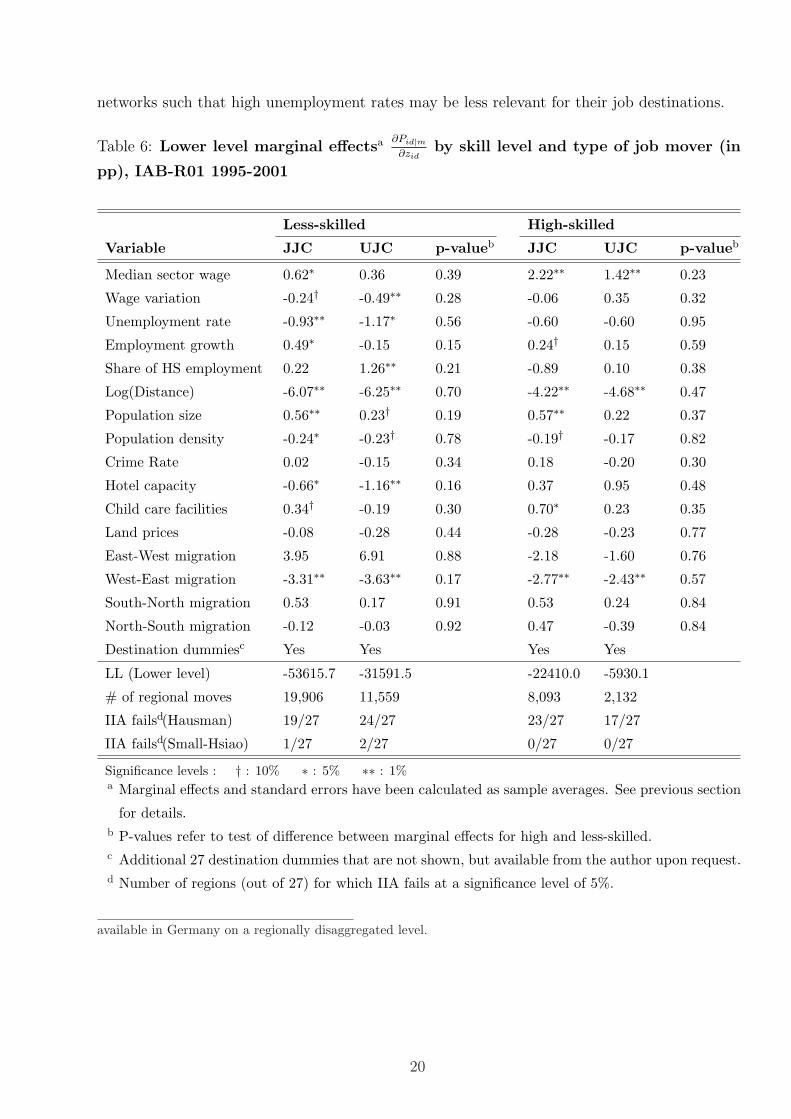
networks such that high unemployment rates may be less relevant for their job destinations.

Table 6: Lower level marginal effectsa ∂Pid|m∂zid

by skill level and type of job mover (in

pp), IAB-R01 1995-2001

Less-skilled High-skilled

Variable JJC UJC p-valueb JJC UJC p-valueb

Median sector wage 0.62∗ 0.36 0.39 2.22∗∗ 1.42∗∗ 0.23

Wage variation -0.24† -0.49∗∗ 0.28 -0.06 0.35 0.32

Unemployment rate -0.93∗∗ -1.17∗ 0.56 -0.60 -0.60 0.95

Employment growth 0.49∗ -0.15 0.15 0.24† 0.15 0.59

Share of HS employment 0.22 1.26∗∗ 0.21 -0.89 0.10 0.38

Log(Distance) -6.07∗∗ -6.25∗∗ 0.70 -4.22∗∗ -4.68∗∗ 0.47

Population size 0.56∗∗ 0.23† 0.19 0.57∗∗ 0.22 0.37

Population density -0.24∗ -0.23† 0.78 -0.19† -0.17 0.82

Crime Rate 0.02 -0.15 0.34 0.18 -0.20 0.30

Hotel capacity -0.66∗ -1.16∗∗ 0.16 0.37 0.95 0.48

Child care facilities 0.34† -0.19 0.30 0.70∗ 0.23 0.35

Land prices -0.08 -0.28 0.44 -0.28 -0.23 0.77

East-West migration 3.95 6.91 0.88 -2.18 -1.60 0.76

West-East migration -3.31∗∗ -3.63∗∗ 0.17 -2.77∗∗ -2.43∗∗ 0.57

South-North migration 0.53 0.17 0.91 0.53 0.24 0.84

North-South migration -0.12 -0.03 0.92 0.47 -0.39 0.84

Destination dummiesc Yes Yes Yes Yes

LL (Lower level) -53615.7 -31591.5 -22410.0 -5930.1

# of regional moves 19,906 11,559 8,093 2,132

IIA failsd(Hausman) 19/27 24/27 23/27 17/27

IIA failsd(Small-Hsiao) 1/27 2/27 0/27 0/27

Significance levels : † : 10% ∗ : 5% ∗∗ : 1%a Marginal effects and standard errors have been calculated as sample averages. See previous section

for details.b P-values refer to test of difference between marginal effects for high and less-skilled.c Additional 27 destination dummies that are not shown, but available from the author upon request.d Number of regions (out of 27) for which IIA fails at a significance level of 5%.

available in Germany on a regionally disaggregated level.

20

We can conclude that interregional economic differences affect the skill composition of inter-

regional job flows for two main reasons. Firstly, higher wage levels disproportionately attract

high-skilled migrants, especially high-skilled job-to-job changers. Secondly, lower unemploy-

ment rates mainly attract less-skilled job seekers. Interregional differences in wage dispersion

further contributes to skill sorting across space, but only plays a secondary role. Employment

growth attracts mainly job-to-job changers irrespective of skill-level, but weakly contributes to

skill-sorting due to a disproportionate share of high-skilled JJC.

Amenities and rents Table 5 contains some indication that high-skilled individuals have

higher amenity valuations than their less-skilled counterparts. In particular, public goods

such as the availability of child care facilities significantly attract only high-skilled job movers

(marginal effect of 0.6pp). Moreover, parameter estimates for the urban scale effect of higher

population levels are not contradictory to the notion that high-skilled individuals have higher

valuations of consumer amenities. Table 6 suggests, however, that evidence in favor of higher

amenity valuation among high-skilled movers almost vanishes when controlling for the type

of job move. Instead, both high-skilled and less-skilled job-to-job movers are significantly

attracted to regions with a favorable child care infrastructure. What is more, point estimates

for the urban scale effect of higher population levels are twice as large for JJC than for UJC

irrespective of skill-level. Although differences between JJC and UJC are not significant20, these

results weakly indicate that JJC may have higher amenity valuations than UJC. Since JJC are

relatively well-educated on average, these preferences also weakly affect the skill sorting across

space. Additional indicators such as regional crime rates or land prices do not significantly

affect skill composition of job flows. Similarly, a higher population density is a comparable

disamenity for all sub-groups and thus also leaves the skill composition mainly unaffected.

Variable migration cost As expected, the likelihood of moving to a region significantly

decreases with distance for all skill levels. Moreover, consistent with the theoretical framework,

migration costs associated with migration distance are higher for less-skilled than for high-

skilled job changers at a 10% significance level. In order to keep the probability of moving to

region k constant if migration distance marginally increases from 100 to 101 km, the hourly

wage level in k has to be 0.02 euros higher for high-skilled and 0.12 euros higher for less-skilled

individuals21. Thus, the proportion of high-skilled following a particular migration path clearly

increases with distance. According to Table 6, this finding is robust if the type of job move is

20In fact, for almost all parameters, establishing significant differences across skill groups turns out to be

difficult due to imprecise estimates for at least one group.21The change in wages that keeps the probability of moving to k constant if distance (km) increases is given

by: ∂wage∂km = ∂wage

∂log(km)∂log(km)

km . Coefficient estimates are not shown, but are available from the author upon

request.

21

controlled for.

For individuals born in West Germany, moving to the eastern part of the country is associ-

ated with a strong and significant disutility and thus additional migration costs. These costs

may partially reflect economic disparities between both parts of Germany that are not captured

by other covariates. Since no other migration paths yield any additional utility or disutility,

however, the other covariates already seem to capture major regional disparities. Therefore,

the disutility of moving to eastern Germany is likely to reflect some reluctance to cross the

former border that is not explicable by observed regional disparities. Such reluctance has also

been found by Buchel et al. (2001) in a study of migration intentions among West Germans.

Only one third of those who are willing to change residential location are also willing to move

to eastern Germany while more than 50% are willing to leave the country. Thus, at least for

individuals born in West Germany, the former border still seems to exist in their minds.

Upper level estimates Table 7 shows marginal effects on the marginal probability of leaving

the local region, i.e. to experience an interregional instead of an intraregional job move. The

estimates include the inclusive value estimate ivim from the lower level specification B. This

inclusive parameter reflects the expected utility that an individual derives from migration. The

corresponding parameter estimate ζ indicates whether pull factors are important in determining

mobility decisions. High-skilled job-to-job changers appear to be more responsive to pull factors

than other sub-groups. As a consequence, the share of interregional movers who are high-skilled

slightly increases if other labor markets gain in attractiveness. Apart from the inclusive value,

there are a number of additional upper level covariates that significantly affect the decision

to change a job interregionally. Across all sub-groups, younger, better skilled and previously

well-earning job changers are more likely to be interregionally mobile. The latter two findings

may both reflect higher migration propensities among individuals with higher skill levels since

the previous wage income is likely to capture some heterogeneity in skills that is unexplained by

formal education. Among the employment history indicators, having previously been recalled

dramatically reduces the likelihood of changing a job interregionally because these individuals

tend to be recalled locally again and may simply not be looking for jobs elsewhere. Longer

average tenure also reduces the probability of leaving the local region, probably due to the

regional attachment that comes with a long job tenure. Furthermore, migration levels increased

during the observation period from 1995 to 2001. This is in line with Heiland (2004) who finds

that increasing migration levels coincided with a period of stagnation in eastern Germany in

the mid to late 1990s. Finally, the estimates suggest a much higher probability of changing

a job interregionally for less-skilled East Germans as compared to West Germans. This may

reflect unfavorable employment conditions that force especially less-skilled individuals in eastern

Germany to look for jobs in alternative locations.

22

Table 7: Upper level marginal effectsa ∂Pim

∂wifor specification B by skill level and type

of job move (in pp), IAB-R01 1995-2001

JJC & UJC JJC UJC

Covariates LS HS LS HS LS HS

Age 25-30 0.86∗ 5.15∗∗ 1.23∗∗ 4.61∗∗ 0.27 5.19∗∗

Age 30-35 1.08∗∗ 4.15∗∗ 1.29∗∗ 3.37∗∗ 0.80∗ 6.81∗∗

Age 40-45 -0.07 -3.90∗∗ -0.11 -4.62∗∗ -0.07 -2.08

UJC -1.92∗∗ 4.66∗∗ n/a n/a n/a n/a

Unskilled -2.07∗∗ n/a -2.32∗∗ n/a -1.51∗ n/a

Born in East Germany 9.27∗ -3.26 9.08† -3.36 9.26∗ -2.60

2nd wage quintile 0.17 -6.27∗∗ 0.01 -7.44∗∗ 0.25 -2.48

3rd wage quintile 2.02∗∗ -2.02∗ 2.69∗∗ -3.31∗∗ 1.29 2.13

4th wage quintile 5.70∗∗ 3.87∗∗ 6.41∗∗ 2.70† 4.27∗∗ 7.54∗∗

5th wage quintile 12.9∗∗ 9.51∗∗ 13.66∗∗ 7.58∗∗ 14.6∗∗ 18.1∗∗

Average tenure -0.75∗∗ -0.87∗∗ -0.78∗∗ -1.05∗∗ -0.67∗∗ 0.22

Mth. non-employed -0.13 -0.50∗ -0.28∗∗ -0.37 -0.05 -0.70∗∗

Prev. recall -16.41∗∗ -20.70∗∗ -3.17∗∗ -6.66∗ -16.3∗∗ -35.5∗∗

1996 -1.00∗ -0.45 -0.44 1.09 -1.18∗ -5.30

1997 -0.43 1.88 -0.18 2.74∗ -0.16 -0.48

1998 0.55 2.38∗ 0.41 2.68∗∗ 1.19† 2.21

1999 0.44 2.69† 0.85 2.93 0.45 2.66

2000 2.06∗∗ 1.82 2.24∗ 1.52 2.49∗∗ 5.14∗

2001 1.86∗∗ 3.29∗ 2.35∗∗ 3.22† 1.93∗∗ 5.17†

Other covariatesb X X X X X X

ζmc 0.31∗∗ 0.47∗∗ 0.28∗∗ 0.46∗∗ 0.34∗∗ 0.29∗∗

LL (upper level) -77495.2 -16892.4 -47106.2 -13473.5 -29812.4 -3335.4

# of job moves 175,587 26,457 95,938 21,040 79,649 5,417

Significance levels : † : 10% ∗ : 5% ∗∗ : 1%

a Marginal effects and standard errors have been calculated as sample averages.

See previous section for details.b Includes 13 sector of activity dummies, 9 types of occupation dummies, 27 origin dummies.

Full estimation results are available from the author upon request.c Displays coefficient estimate instead of marginal effect.

Simulation Results Based on the preceding estimation results, this section simulates how

the level and skill composition of job matching flows changes in a scenario of economic con-

23

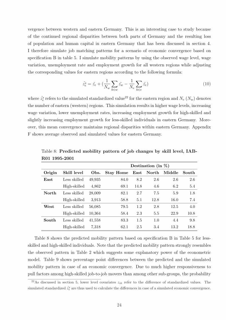
vergence between western and eastern Germany. This is an interesting case to study because

of the continued regional disparities between both parts of Germany and the resulting loss

of population and human capital in eastern Germany that has been discussed in section 4.

I therefore simulate job matching patterns for a scenario of economic convergence based on

specification B in table 5. I simulate mobility patterns by using the observed wage level, wage

variation, unemployment rate and employment growth for all western regions while adjusting

the corresponding values for eastern regions according to the following formula:

zse = ze + (

1

Nw

∑

k∈w

zw − 1

Ne

∑

k∈e

ze) (10)

where zse refers to the simulated standardized value22 for the eastern region and Ne (Nw) denotes

the number of eastern (western) regions. This simulation results in higher wage levels, increasing

wage variation, lower unemployment rates, increasing employment growth for high-skilled and

slightly increasing employment growth for less-skilled individuals in eastern Germany. More-

over, this mean convergence maintains regional disparities within eastern Germany. Appendix

F shows average observed and simulated values for eastern Germany.

Table 8: Predicted mobility pattern of job changes by skill level, IAB-

R01 1995-2001

Destination (in %)

Origin Skill level Obs. Stay Home East North Middle South

East Less skilled 49,935 84.0 8.2 2.6 2.6 2.6

High-skilled 4,862 69.1 14.8 4.6 6.2 5.4

North Less skilled 28,009 82.1 2.7 7.5 5.9 1.8

High-skilled 3,913 58.8 5.1 12.8 16.0 7.4

West Less skilled 56,085 79.5 1.2 2.8 12.5 4.0

High-skilled 10,364 58.4 2.3 5.5 22.9 10.8

South Less skilled 41,558 83.3 1.5 1.0 4.4 9.8

High-skilled 7,318 62.1 2.5 3.4 13.2 18.8

Table 8 shows the predicted mobility pattern based on specification B in Table 5 for less-

skilled and high-skilled individuals. Note that the predicted mobility pattern strongly resembles

the observed pattern in Table 2 which suggests some explanatory power of the econometric

model. Table 9 shows percentage point differences between the predicted and the simulated

mobility pattern in case of an economic convergence. Due to much higher responsiveness to

pull factors among high-skilled job-to-job movers than among other sub-groups, the probability

22As discussed in section 5, lower level covariates zik refer to the difference of standardized values. The

simulated standardized zse are thus used to calculate the differences in case of a simulated economic convergence.

24

of leaving the local region strongly increases for high-skilled individuals in western states and

strongly decreases in eastern states compared to much weaker reactions for their less-skilled

counterparts. More importantly, economic convergence attracts job movers of all skill levels

and from all regions to eastern Germany. Pull factors are again much stronger for high-skilled

than for less skilled individuals however. In fact, the probability of moving to the eastern states

more than triples for high-skilled individuals, but less than doubles for less-skilled individuals.

Table 9: Simulated change in the spatial pattern of job movements by

skill level in case of an economic convergence between western and

eastern Germany, IAB-R01 1995-2001

Destination (pp change)

Origin Skill level Obs. Stay Home East North Middle South

East Less skilled 49,935 1.38 2.15 -1.18 -1.18 -1.18

High-skilled 4,862 5.27 6.41 -3.31 -4.47 -3.91

North Less skilled 28,009 -0.85 2.58 -0.92 -0.61 -0.21

High-skilled 3,913 -4.97 14.92 -3.61 -4.23 -2.10

Mid Less skilled 56,085 -0.39 1.42 -0.17 -0.62 -0.24

High-skilled 10,364 -2.55 8.69 -0.90 -3.49 -1.75

South Less skilled 41,558 -0.47 1.58 -0.08 -0.31 -0.72

High-skilled 7,318 -2.86 9.03 -0.63 -2.27 -3.27

As a consequence, economic convergence affects net job flows between both parts of Germany

and changes the skill composition of west-east and east-west flows as can be seen in Table 10.

Besides looking at the effects of a full economic convergence as described above, Table 10

also identifies the main sources of the simulated change by looking at the effects in case of

an isolated convergence of wage levels, wage dispersion, unemployment rates and employment

growth, respectively. As suggested by the previous estimation results, the increasing skill-level

of west-east flows from 23.5% to 39.6% in case of a full economic convergence is mainly driven by

increasing wage levels in eastern states. Higher wage inequality in eastern regions also increases

the skill level of west-east flows. This is due, however, to an increasing net outflow of less-skilled

job movers. By contrast, converging wage levels not only strongly increase the share of high-

skilled west-east migrants, but also substantially raise net migration as has also been suggested

by Burda and Hunt (2001). In case of full convergence, it is mainly lower unemployment levels

that further raises the number of net migrants, mainly due to an increased net migration of

less-skilled job changers. Thus, while higher wage levels turn out to be an effective means of

attracting human capital to eastern Germany, the net outflow from eastern to western regions

can only be reversed by a combination of higher wage levels and lower unemployment rates.

25

Table 10: Net job flows, induced net employment change by skill level and

share of high-skilled migrants for various scenarios, IAB-R01 1995-2001

Net migration Net emp. change Share HS migrants

LS HS LS HS east-west west-east

Observed -1,447 -183 -1.4 % -1.2 % 16.5 % 18.7 %

Predicted -1,847 -154 -1.8 % -1.0 % 16.7 % 23.5 %

Isolated convergence of

Wage level -376 1,675 -0.4 % 10.7 % 8.9 % 41.9 %

Wage variance -2,812 -134 -2.7 % -0.9 % 14.7 % 27.8 %

Unemployment rate 1,505 247 1.5 % 1.6 % 21.1 % 18.5 %

Employment growth -1,803 -99 -1.7 % -0.6 % 16.4 % 24.2 %

Full convergence 2,096 2,559 2.0 % 16.4 % 9.2 % 39.6 %

Note: Employees by skill level are computed based on the IAB-R01 at the beginning

of the observation period (01/01/1995).

7 Conclusion

Regional economic prospects critically hinge on the skill composition of internal migration

flows. Given the brain drain from eastern to western Germany, understanding what drives the

skill composition of migration flows is of particular interest in the German context. By look-

ing at destination choice patterns of heterogenous job movers, this paper has identified major

determinants of the skill composition of internal job matching flows in Germany. As another

contribution, this study has also shown that this skill composition is partially driven by differ-

ent destination choice patterns of job-to-job changers and job changers after unemployment.

Moreover, including destination fixed effects in the destination choice analysis proved impor-

tant to avoid biases arising from the omission of unobserved regional characteristics. Using a

partially degenerate nested logit analysis, this paper comes to the following main conclusions:

• Interregional income differentials affect the skill composition of job matching flows mainly

because high-skilled job movers are much more responsive to interregional variation in

the wage level than their less-skilled counterparts. There is also evidence consistent with

the Roy model that less-skilled individuals avoid destinations with high wage inequality.

• Job-finding conditions affect the skill composition of migration flows because only less-

skilled individuals avoid destinations with high unemployment rates.

26

• Higher amenity valuations of job-to-job changers compared to job changers after unem-

ployment weakly contribute to skill sorting across space since a higher share of job-to-job-

movers is high-skilled. There is no evidence in favor of higher amenity valuations among

high-skilled job movers when controlling for the type of job move.

• High-skilled job movers face lower migration costs such that the proportion of high-skilled

migrants strongly increases with migration distance.

• High-skilled job-to-job movers are more responsive to pull factors than all other sub-

groups. Improving destination conditions thus disproportionately mobilize this group

which affects the skill composition of internal job matching flows.

These findings imply that rising wage levels in eastern Germany during the 1990s have

been an effective means of preventing a stronger brain drain. However, wages have risen at

the cost of higher unemployment levels which mainly boosted east-west migration of less-skilled

individuals. Simulated economic convergence between eastern and western Germany shows that

higher wage levels are the most effective means of attracting human capital to eastern Germany,

but that the net loss of population can only be reversed by a combination of higher wage levels

and lower unemployment rates. If maintaining the future viability of eastern Germany is a

pronounced policy objective, the findings in this paper thus advocate policies that foster wage

convergence without further increasing eastern unemployment levels. For this purpose, policy

measures such as continued infrastructure investments that help in closing the productivity gap

between eastern and western Germany may be a first choice.

Finally, the study points to a number of upcoming research tasks. First of all, using a

nested logit approach is restrictive due to its reliance on the IIA assumption. Since the evidence

regarding the appropriateness of this assumption is mixed, the findings should be compared to

less restrictive specifications such as a multinomial probit. Secondly, heterogeneous destination

choice patterns point to the need to extend the analysis to endogenously model the job mobility

decision since the composition of job movers may change with labor market conditions. If job-

to-job movers are more prevalent in boom periods, for example, job matching patterns and

thus also the interregional competition for jobs may differ across the business cycle. Finally,

due to data restrictions, the analysis leaves out highly mobile and important labor segments,

namely single females and university graduates. Future research should examine destination

choice patterns of these segments because they strongly affect the skill composition of internal

job matching flows.

27

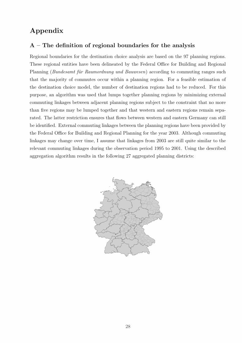
Appendix

A – The definition of regional boundaries for the analysis

Regional boundaries for the destination choice analysis are based on the 97 planning regions.

These regional entities have been delineated by the Federal Office for Building and Regional

Planning (Bundesamt fur Raumordnung und Bauwesen) according to commuting ranges such

that the majority of commutes occur within a planning region. For a feasible estimation of

the destination choice model, the number of destination regions had to be reduced. For this

purpose, an algorithm was used that lumps together planning regions by minimizing external

commuting linkages between adjacent planning regions subject to the constraint that no more

than five regions may be lumped together and that western and eastern regions remain sepa-

rated. The latter restriction ensures that flows between western and eastern Germany can still

be identified. External commuting linkages between the planning regions have been provided by

the Federal Office for Building and Regional Planning for the year 2003. Although commuting

linkages may change over time, I assume that linkages from 2003 are still quite similar to the

relevant commuting linkages during the observation period 1995 to 2001. Using the described

aggregation algorithm results in the following 27 aggregated planning districts:

28

B – Definition and data sources of lower-level covariates

Variable Definition 1 yr Lag Data Sourcea

Covariates with area and individual variation

Median sector wage Median wage in individual i’s sector of ac-

tivity l (l = 1..13)

No A

Sector employment

growthb

Biennial employment growth in individual

i’s skill group

Yes B

Covariates with area variation

Wage variance index Regional wage quantile ratio divided by

aggregate quantile ratio

No A

Unemployment rate Average yearly unemployment rate Yes C

Share HS employment Share of high-skilled employment Yes B

Log(Distance) Log of average distance between all county

capitals of any two regions

- D

Population size Number of residents in 100,000 Yes E

Population density Number of residents (in 100) per km2 Yes E

Crime Rate Total offenses per 100 residents No F

Hotel capacity Number of hotel beds per 1000 residents No E

Child care facilities Places in day care for children and youth

per 1,000 residents

No E

Land prices Land prices in 100 euros per m2 No Ea A - Own calculation based on IAB-R01 1995-2001. See Appendix C for details on the calculation.

B - Own calculation based on IAB-R01 1993-2001

C - Federal Employment Agency (Bundesagentur fur Arbeit)

D - Own calculations based on the grid position of county capitals

E - Federal Statistical Office (Statistisches Bundesamt)

F - European Regional Crime Database, Entorf und Spengler (2004)b I distinguish between employment growth for high-skilled and less-skilled individuals.

C – Estimating moments of the regional wage distribution

The observed regional wage distribution reflects interregional differences in both skill prices

and skill mix. For this reason, Hunt and Mueller (2002) control for interregional differences

in the skill mix by estimating key parameters of a standardized regional wage distribution

that is comparable across regions. Mainly following their methodology, I separately estimate

Mincerian-type wage equations for each region k based on the IAB-R01. Since wages in the

IAB-R01 are top-coded at the income level above which there is no obligation to be socially

insured, I estimate a tobit model. I restrict the estimation to prime age males who are full-time

employed on January 1st and include educational attainment, experience, occupation type and

29

sector of activity as covariates. I predict the standardized wage distribution for region k by

using the entire sample of prime age males and the coefficient estimates for region k. Since

the same sample is applied to each region, this procedure controls for interregional differences

in skills and experience levels and thus yields a standardized wage distribution. Due to the

censoring in the data, it is not possible to consistently estimate the moments of this standardized

distribution. For this reason, I use percentiles which are unaffected by the censoring of the data

to appropriately measure interregional wage differences. Therefore, I estimate the median wage

by sector of activity as an indicator of interregional differences in the sector-specific wage levels.

As an indicator of the wage variance in region k, I calculate the difference between the 80th

and 20th wage quantile based on the standardized wage distribution for region k and divide it

by the corresponding quantile ratio of the wage distribution when pooling all regions. If this

wage variance index is larger than 1, the wage inequality in region k exceeds the average wage

inequality.

D – Sample averages for lower level covariates by sub-sample

JJC UJC

Covariates LS HS LS HS

Median sector wage 0.104 0.055 0.139 0.110

Wage variance index 0.066 0.013 0.085 0.034

Unemployment rate -0.114 -0.057 -0.146 -0.137

Employment growth 0.026 0.028 0.038 0.043

Share of HS employment -0.009 0.028 -0.009 0.125

Log(Distance) 5.163 5.307 5.209 5.276

Population size 0.012 0.014 0.022 0.050

Population density 0.014 0.003 0.041 0.032

Crime Rate -0.051 -0.020 -0.066 -0.060

Hotel capacity 0.010 0.002 -0.019 0.012

Child care facilities -0.048 0.006 -0.062 -0.050

Land prices 0.094 0.071 0.122 0.205

# of interregional moves 19,906 8,093 11,559 2,132

∗ Except for log(distance), all covariates refer to the difference between the standardized

value for the destination (d) and the origin (o) region. Thus a value of 1 indicates a

difference of one standard deviation between d and o.∗∗ JJC - Job-to-job changer; UJC - Job changers after unemployment; LS - Less-skilled; HS

- High-skilled

30

E – Sample averages for upper level covariates by sub-sample

JJC UJC

Covariates LS HS LS HS

Migrant 0.21 0.38 0.15 0.39

Age (Reference: Age 30-35)

25-30 0.29 0.15 0.27 0.13

30-35 0.29 0.37 0.27 0.32

40-45 0.19 0.20 0.22 0.26

Wage quintile in previous joba(Reference: 1st wage quintile)

2nd 0.25 0.08 0.31 0.18

3rd 0.16 0.09 0.17 0.15

4th 0.10 0.19 0.07 0.17

5th 0.07 0.39 0.02 0.19

Employment history and other covariates

Born in East Germany 0.21 0.13 0.33 0.22

Multiple job changesb 0.73 0.71 0.85 0.73

Prev. average tenure (yrs.) 2.91 2.44 1.74 1.76

Months prev. non-employed 1.04 0.76 2.24 1.97

Prev. recall by employer 0.01 0.01 0.18 0.03

Previous sector of activity (Reference: Agriculture and Fishing)

Primary industry 0.06 0.05 0.06 0.04

Invest. goods/engineering 0.08 0.08 0.05 0.07

Invest. goods/vehicles 0.07 0.11 0.04 0.07

Cons. goods/ food process. 0.07 0.04 0.07 0.04

Construction 0.17 0.05 0.37 0.10

Wholesale trade 0.08 0.07 0.05 0.07

Retail 0.07 0.03 0.05 0.04

Transport/Communication 0.10 0.03 0.06 0.03

Financial services 0.17 0.32 0.09 0.22

Domestic services 0.05 0.02 0.04 0.03

Social services 0.04 0.15 0.05 0.22

Public authorities 0.01 0.02 0.02 0.04

Previous type of occupation (Reference: Agricultural work

Blue-collar work 0.51 0.05 0.66 0.12

Salesmen 0.07 0.06 0.04 0.06

Technical work 0.06 0.35 0.03 0.29

Clerical work 0.06 0.11 0.03 0.10

White-collar work 0.05 0.26 0.02 0.16

Health-related/Teaching/Consulting 0.02 0.12 0.01 0.18

Other service jobs 0.20 0.05 0.16 0.07

Year of job move (Reference: 1995)

1996 0.13 0.11 0.15 0.14

1997 0.13 0.12 0.17 0.15

1998 0.13 0.14 0.15 0.15

1999 0.15 0.17 0.15 0.15

2000 0.16 0.18 0.13 0.13

2001 0.15 0.18 0.13 0.13

# of job moves 95,935 21,040 79,649 5,417

a Wage quintiles of the wage distribution of all full time employees observed on January 1st of each year (Data: IAB-R01).c Indicator whether an individual contributes two or more observations (i.e. job changes) to the sample.d The duration of the previous spell refers to the previous job tenure for JJC and to the unemployment period for UJC.

31

F – Average observed and simulated unemployment rate, wage level,

wage dispersion and employment growth for eastern Germany

Indicator 1Ne

∑k∈e zs

e1

Ne

∑k∈e ze

Median wage in agriculture 0.50 -1.75

Median wage in primary ind. 0.49 -1.73

Median wage in inv. good/engineering 0.49 -1.70

Median wage in inv. goods ind./vehicles 0.48 -1.69

Median wage in cons. goods/food process. 0.50 -1.74

Median wage in construction 0.52 -1.80

Median wage in wholesale trade 0.48 -1.68

Median wage in retail 0.47 -1.70

Median wage in transport/communication 0.48 -1.69

Median wage in financial services 0.50 -1.76

Median wage in domestic services 0.42 -1.47

Median wage in social services 0.50 -1.76

Median wage in public authorities 0.47 -1.66

Wage variance 0.46 -1.62

Unemployment rate -0.46 1.60

Emp. growth for less-skilled jobs -0.39 -0.56

Emp. growth for high-skilled jobs 1.02 0.25

Note: Average simulated values for eastern regions correspond to the ob-

served average values for western regions, i.e. 1Ne

∑k∈e zs

e = 1Nw

∑k∈w zw.

32

References

[1] Amemiya, T. (1978). On two-step Estimation of Multivariate Logit-models. Journal of

Econometrics Vol. 8, 13-21.

[2] Arntz, M. (2005). The Geographical Mobility of Unemployed Workers. Evidence from West

Germany. ZEW Discussion Paper No.05-34.

[3] Arntz, M. Boeters, S. and N. Gurtzgen (forthcoming). Alternative Approaches to Discrete

Working Time Choice in an AGE Framework. Economic Modelling

[4] Bartel, A.P. (1979). The Migration Decision: What Role Does Job Mobility Play? The

American Economic Review Vol. 69, 775-786.

[5] Borjas, G.J. (1987). Self-Selection and the Earnings of Immigrants. American Economic

Review Vol. 77, 1667-1717.

[6] Borjas, G.J., Bronars, S.G. and S.J. Trejo (1992). Self-Selection and Internal Migration in

the United States. Journal of Urban Economics Vol. 32, 159-185.

[7] Brucker, H. and P. Trubswetter (2004). Do the Best Go West? An Analysis of the Self-

Selection of Employed East-West Migrants in Germany. IZA Discussion Paper No. 986 Bonn.

[8] Bruckner, J.K., Thisse, J.-F. and Y. Zenou (1999). Why is Central Paris Rich and Downtown

Detroit Poor? An Amenity-Based Theory. European Economic Review Vol. 43, 91-107.

[9] Buchel, F., Frick, J.R. and J.C. Witte (2002). Regionale und berufliche Mobilitat von

Hochqualifizierten - ein Vergleich Deutschland - USA. In: Bellmann, L.; Velling, J. (eds.).

Arbeitsmarkte fur Hochqualifizierte. Nurnberg: IAB, 207-243.

[10] Burda, M.C. (1993). The Determinants of East-West German Migration - Some First

Results. European Economic Review Vol. 37, 452-461.

[11] Burda, M.C. and J. Hunt (2001). From Reunification to Economic Integration: Produc-

tivity and the Labor Market in Eastern Germany. Brookings Papers on Economic Activity

Vol. 2001(2), 1-71.

[12] Camagni, R.P. (1995). The Concept of Innovative Milieu and Its Relevance for the Lagging

Regions in the 1990s. Papers in Regional Science Vol. 74, 317-340.

[13] Chiswick, B.R. (2000). Are Immigrants Favourably Self-Selected? An Economic Analysis.

IZA Discussion Paper No. 131. Bonn.

33

[14] Ciccone, A. and R.E. Hall (1996). Productivity and the Density of Economic Activity. The

American Economic Review. Vol. 86(1), 54-70.

[15] Daly, A. (1987). Estimating ”Tree” Logit Models. Transportation Research Part B Vol.

21, 251-267.

[16] Davies, P.S., Greenwood, M.J. and H. Li (2001). A Conditional Logit Approach to U.S.

State-to-State Migration. Journal of Regional Science Vol. 41(2), 337-360.

[17] Entorf, H. and H. Spengler (2004). European Regional Crime Database, Darmstadt Uni-

versity of Technology.

[18] Fitzenberger, B. and R.A. Wilke (2004). Unemployment Durations in West-Germany Be-

fore and After the Reform of the Unemployment Compensation System During the 1980s.

ZEW Discussion Paper No. 04-24.

[19] Fitzenberger, B., Osikominu, A. and R. Volter (2005). Imputation Rules to Improve the

Education Variable in the IAB Employment Subsample. ZEW Discussion Paper No. 05-10.

[20] Glaeser, E.L., Kolko, J. and A. Saiz (2001). Consumer City. Journal of Economic Geogra-

phy Vol. 1, 27-50.

[21] Hamann, S. et al. (2004). Die IAB-Regionalstichprobe 1975-2001: IABS-R01. ZA-

Information 55, Zentralarchiv fur Empirische Sozialforschung (Hrsg.), Universitat zu Koln,

S. 34-59.

[22] Heiland, F. (2004). Trends in East-West German Migration from 1989 to 2002. Demo-

graphic Research Vol. 11, Art. 7.

[23] Heiss, F. (2002). Stuctural Choice Analysis with Nested Logit Models. The Stata Journal

Vol. 2(3), 227-252.

[24] Hensher, D.A. and W.H. Greene (2002). Specification and Estimation of the Nested Logit

Model: Alternative Normalisations. Transportation Research Part B Vol. 36, 1-17.

[25] Herzog, H.W. and A.M. Schlottmann (1993). Valuing Amenities and Disamenities of Urban

Scale: Can Bigger Be Better? Journal of Regional Science 33, 145-165.

[26] Hunt, G.L. and R.E. Mueller (2002). A Methodology For Estimating Returns To Skills For

Canadian Provinces and US States. Journal of Regional Science Vol. 42(1), 127-143.

[27] Hunt, G.L. and R. E. Mueller (2004). North American Migration: Returns to Skill, Border

Effects, And Mobility Costs. The Review of Economics and Statistics Vol. 86(4), 988-1007.

34

[28] Hunt, J. (2000). Why do People Still Live in East Germany? DIW Discussion Paper

No.201.

[29] Hunt, J. (2004). Are Migrants More Skilled than Non-Migrants? Repeat, Return and

Same-Employer Migrants. DIW Discussion Paper No. 422.

[30] Koppelman, F.S. and C.-H. Wen (1998). Alternative Nested Logit Models: Stucture, Prop-

erties and Estimation. Transportation Research Part B Vol. 32(5), 289-298.

[31] Krohnert, S., Medicus, F. and R. Klingholz (2006). Die demografische Lage der Nation.

Wie zukunftsfahig sind Deutschlands Regionen? DTV, Berlin.

[32] Krugman, P. (1991). Increasing Returns and Economic Geography. Journal of Political

Economy Vol. 99(3), 483-499.

[33] Lee, S. and R.A. Wilke (2005). Reform of Unemployment Compensation in Germany: A

Nonparametric Bounds Analysis using Register Data. ZEW Discussion Paper No. 05-29.

[34] Lucas, R.E. (1988). On the Mechanics of Economic Development. Journal of Monetary

Economics Vol. 22, 3-42.

[35] Maillat, D. (1998). Innovative Milieux and New Generations of Regional Policies. En-

trepreneurship and Regional Development Vol. 1, 1-16.

[36] McFadden, D. (1978). Modelling the Choice of Residential Location. In: Karlqvist, A.,

Lundqvist, L., Snickars, F. and J.W. Weibull (Eds.) Spatial Interaction Theory and Planning

Models. Amsterdam.

[37] McFadden, D. (1981). Econometric Models of Probalbilistic Choice. In: Manski, C.F. and

D. McFadden (Eds.) Structural Analyses of Discrete Data with Econometric Applications.

Cambridge.

[38] Molho, I. (1987). The Migration Desision of Young Men in Great Britain. Applied Eco-

nomics Vol. 19, 221-243.

[39] Moulton, B.R. (1990). An Illusration of a Pitfall in Estimating the Effects of Aggregate

Variables on Micro Units. Review of Economics and Statistics Vol. 72(2), 334-338.

[40] Nijkamp, P. and J. Poot (1997). Endogenous Technological Change, Long Run Growth

and Spatial Interdependence: A Survey. In: Bertugilia, C., Lombardo, S. and P. Nijkamp

(Eds.) Innovative Behaviour in Space and Time. Springer-Verlag. Berlin.

[41] Rauch, J.E. (1993). Productivity Gains from Geographic Concentration of Human Capital:

Evidence from the Cities. Journal of Urban Economics Vol. 34, 380-400.

35

[42] Ritsila, J and M. Ovaskainen (2001). Migration and Regional Centralization of Human

Capital. Applied Economics Vol. 33, 317-325.

[43] Ritsila, J. and M. Haapanen (2003). Where Do the Highly Educated Migrate? Micro-Level

Evidence from Finland. International Review of Applied Economics Vol. 17(4), 437-448.

[44] Romer, P.M. (1990). Endogenous Technological Change Journal of Political Economy Vol.

98, 71-102.

[45] Roy, A.D. (1951). Some Thoughts on the Distribution of Earnings. Oxford Economic Papers

Vol. 3(2), 135-146.

[46] Schundeln, M. (2002). Migration of Natives and Foreigners Within Germany: Respon-

siveness to Labor Market Differentials and Cost of Migration. Conference Paper from the

UNU/WIDER Conference on Poverty, International Migration and Asylum in Helsinki.

[47] Schwarze, J. (1996). Beeinflusst das Lohngefalle zwischen Ost- und Westdeutschland das

Migrationsverhalten der Ostdeutschen? Eine mikrookonomische Untersuchung mit Daten des

Sozio-okonomischen Panels 1991 bis 1994. Allgemeines Statistisches Archiv Vol. 80, 50-68.

[48] Shaw, C. (1975). The Value of Time. Social and Economic Studies Vol. 42,556-563.

[49] Simon, C.J. (1998). Human Capital and Metropolitan Employment Growth. Journal of

Urban Economics Vol. 43, 223-243.

[50] Small, K.A. and C. Hsiao (1985). Multinomial Logit Specification Tests. International

Economic Review Vol. 26(3), 619-627.

[51] Train, K.E. (2002). Discrete Choice Methods with Simulation. Cambridge University Press,

Cambridge.

36