W E N -S ON C H IA N G S -H C H E N

W -C YA N G J -W L A I K - I L IN E -Y L IA N G

TA I WA N OC E A N RE S E A R C H IN S T I T U T E ,N ATION AL A PPLIED RE SE A RCH L AB ORATORIE S ,

TA IWA N

Preliminary progress of ocean surface current mapping system in

Taiwan

Outline

Initiation of HFR network projectSetup of HFR stationsInstrumentsHFR data analysisValidations of HFR dataApplications

Ocean surface current patternHindcast of drifter trajectories

Summary

Introduction

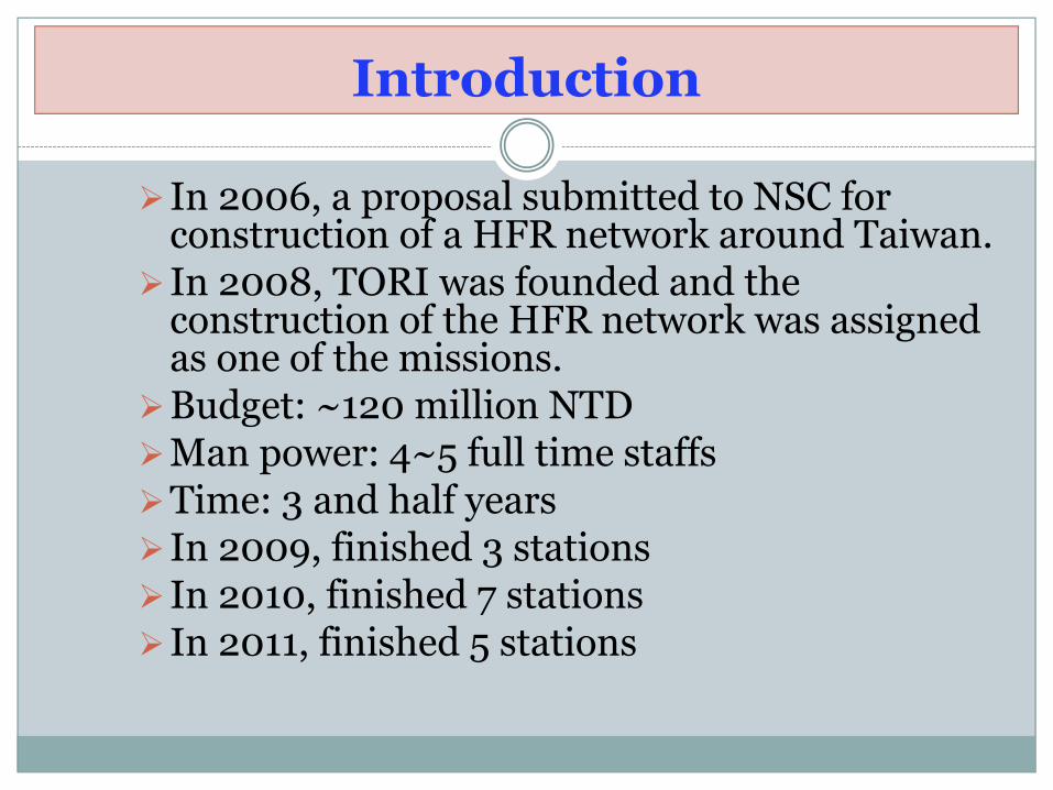
In 2006, a proposal submitted to NSC for construction of a HFR network around Taiwan.In 2008, TORI was founded and the construction of the HFR network was assigned as one of the missions. Budget: ~120 million NTDMan power: 4~5 full time staffsTime: 3 and half yearsIn 2009, finished 3 stationsIn 2010, finished 7 stationsIn 2011, finished 5 stations

Site selection

Guide lines of site selection:1. proximity to water2. the area around the receive antenna should be kept

clear3. enough distance between antennas.4. suitable distance between sites5. power supply6. internet service7. security

Setup of antennas

Once the potential sites had been selected. Before the construction, the most critical thing was to negotiate with owners of the land properties of radar sites:

Coast guardNavyNational companiesCentral and Local governments

List of instruments in each local center:

2 air conditions and auto switch system

a transmitter and a receiver

remote power control system

radar computer

disk array

video recorder

1.5 KVA power supply

local control center

Outdoor type rack with shielding light steel frame

Types of local control center

Container Bunker

Types of local control center

Data Transmission

Data: 75GB per dayOnly small part of that is transmitted through internet.

coverage of HFR ocean surface currents

coverage

red circles : long range sitesred squares : standard sitesshaded area :

120km for the long range radars40km for the standard type radars

Parameters of each radar system

Site Frequency(MHz)

Band Width(kHz)

Resolution(Km)

MeasureRange(km)

Bearing (azimuth)

LUYE 4.58 15 → 40 10 → 3.75 180 59-191SHIA 4.58 15 → 40 10 → 3.75 180 26-186HOPE 4.58 15 → 40 10 → 3.75 180 26-196LIUK 4.58 15 → 40 10 → 3.75 150 235-0DATN 4.58 15 → 40 10 → 3.75 150 57-195TUTL 4.58 15 → 40 10 → 3.75 160 252-2CIHO 4.58 15 → 40 10 → 3.75 170 151-331

HOWN 4.58 15 → 40 10 → 3.75 160 192-327PETI 4.58 15 → 40 10 → 3.75 150 221-332TWIN 4.58 15 → 40 10 → 3.75 180 224-349SUHI 4.58 15 → 40 10 → 3.75 180 178-48LILY 13.425 100 1.5 70 320-110CIAO 13.425 100 1.5 60 359-4MABT 24.3 100 1.5 40 112-256BABY 24.3 100 1.5 40 177-253

According to the hardware of the systems and the local environment, the following parameters were set for each radar site.

Theoretical background of HFR

Bragg scattering off the ocean surfaceDoppler EffectfD =2 V /V = c + ULinear wave :Velocity can be estimatedfrom frequency shift basedon the returned signalspectrum. According tolinear wave theory, thephase velocity wasseparated from oceancurrent

2gc

Radial sectors of each radar site

Concept of Velocity combination

radial

• Clean radial( > 260 cm/s depends on each site)• Radial grid(dR=10(2)km; dD=5deg)• Radial interpolation

total

• define total grid (0.1 degree)• exclude the total grids out of the bearing• search radial vector for each total grid (Dist < 15km)• at least 2 sites and 3 radial vectors for

combination of total velocity• GDOP >1.25 (30 < cross angle <150)• Least square method

smooth • Spatial interpolation• Temporal interpolation

Parameters of Data Analysis

Total velocity

Search range effect

Xradius=9km Xradius=20km

• GDOP: 1.25 (cross angle between 30~150 degree), leftGDOP: 1.00 (cross angle between 20~160 degree), right

Geometric dilution of position(GDOP ) effect

Comparison between ideal and measured pattern

ideal pattern measured pattern

Resolution(Km)

Radials around each grid point.

(km)

Maximuncurrentvelocity(cm/s)

GDOP( O )

ALML(Long Range)

10 20 200 30

SOUTH(Standard)

1.5 2 180 30

NORTH(Standard)

1.5 2 180 30

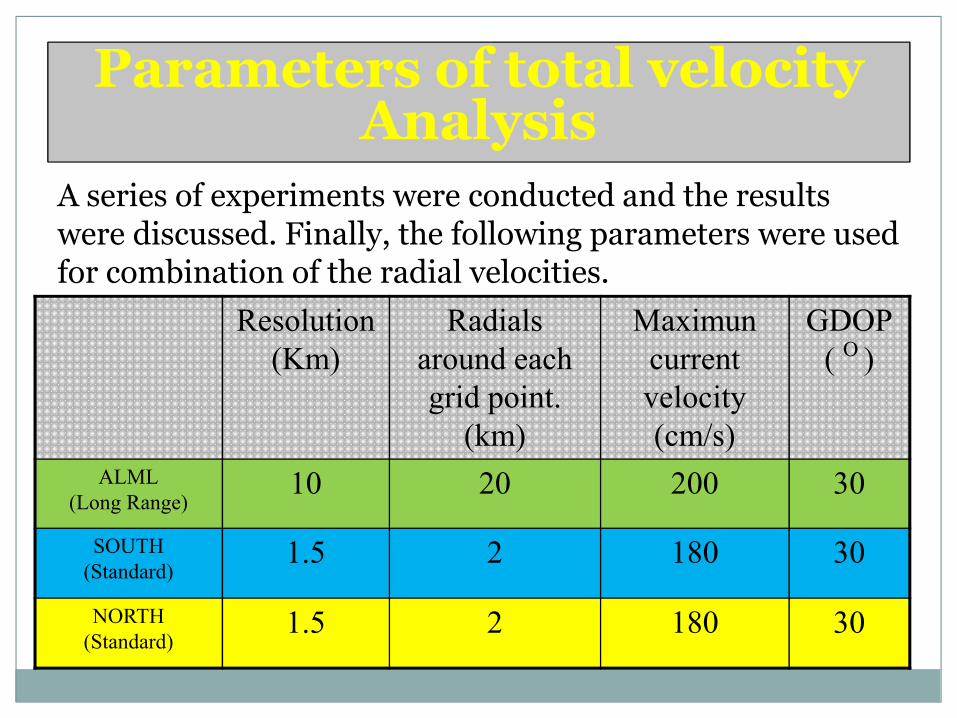
Parameters of total velocity Parameters of total velocity Analysis

A series of experiments were conducted and the results were discussed. Finally, the following parameters were used for combination of the radial velocities.

coverage of good data percentage

coverage of good data percentage based on data from the Jan. 1 and Nov. 30 in 2012

Validation of HFR surface currents

Totally, 8 drifters were deployed in 2012, which trajectories are shown on the right panel.

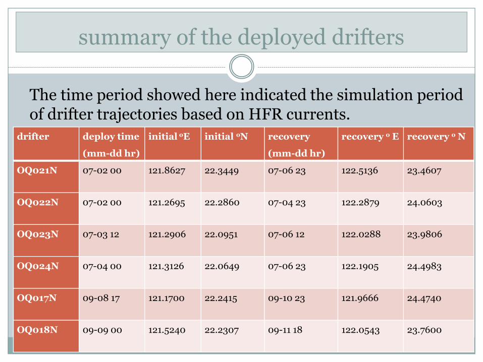
summary of the deployed drifters

drifter deploy time

(mm-dd hr)

initial oE initial oN recovery

(mm-dd hr)

recovery o E recovery o N

OQ021N 07-02 00 121.8627 22.3449 07-06 23 122.5136 23.4607

OQ022N 07-02 00 121.2695 22.2860 07-04 23 122.2879 24.0603

OQ023N 07-03 12 121.2906 22.0951 07-06 12 122.0288 23.9806

OQ024N 07-04 00 121.3126 22.0649 07-06 23 122.1905 24.4983

OQ017N 09-08 17 121.1700 22.2415 09-10 23 121.9666 24.4740

OQ018N 09-09 00 121.5240 22.2307 09-11 18 122.0543 23.7600

The time period showed here indicated the simulation period of drifter trajectories based on HFR currents.

Comparisons of measured and estimated velocitydrifter OQ021N

Drifted to northeastern direction driven by the KuroshioA periodic velocity oscillation due to wind forcingCurved trajectory affected by the eddy transportationexperienced a small scale

flow circulation

Wind speed

bathymetry

Comparisons of measured and estimated velocitydrifter OQ022N

07/02 07/03 07/04 07/050

5

10

month/day

win

d ve

loci

ty(m

/s)

Drifted to northeastern direction driven by the KuroshioLarge velocity difference was found due to decreasing water depth

topography change dramatically

Wind speed

bathymetry

Comparisons of measured and estimated velocitydrifter OQ023N

Drifted to northeastern direction driven by the KuroshioHigh frequency velocity oscillation was found near the trench. HFR can not reveal the high frequency speed variation in time.

near the Green Island

Wind speed

bathymetry

R= 0.7051 (Xr=9 km)generally fall along the line of unit slopesome uncertainties as represented by scattering of the data pointsHFR velocities were weaker

？ reasonsDifferent system Uncertaintyerror

Comparisons of velocities at drifter locations

Consider only the “measured” data

Experiences learned form these experiments

Limitation of the spatial resolution small scale eddy can not be resolved.High frequency oscillations of velocity due to the dramatic change of bathymetry was not found in HFR currents.Surface currents derived based on HFRs was generally weaker than that of drifters, especially at the region where the dramatic change of bathymetry was found.

Applicationocean surface current off eastern Taiwan

Codar results: Dec. 2011 ~ Jul. 2012 Hsin et al.(2008)

Seasonal Cycledata measured during 1991-2000

Liang et al., Deep Sea Research II, Vol. 50, 2003

Seasonal variation of ocean surface current off eastern Taiwan

Monthly mean current (a)Jan. (b)Mar. (c)May (d)July

month 2012-07

The Kuroshio flows along the east coast of Taiwan and splits into two branches.One branch flows northward follows the east coastline of Taiwan. The other goes northeastward through OGC into the basin of Pacific Ocean. Flow strength of the two branches varies in time.

Detide currents

The low frequency currents were derived by a low-pass filter (>33Hr).The variation of low frequency currents versus time was shown on the right figure.Demonstrated the wind driven current on the ocean surface.

Applicationocean surface currents induced by a typhoon event

Left column:hourly current velocity field Right column:weather radar images

The figures revealed the variations of ocean surface current pattern corresponded to the movement of the typhoon, which indicated the potential use of HFR currents to the study of air-sea interaction induced by typhoon events.

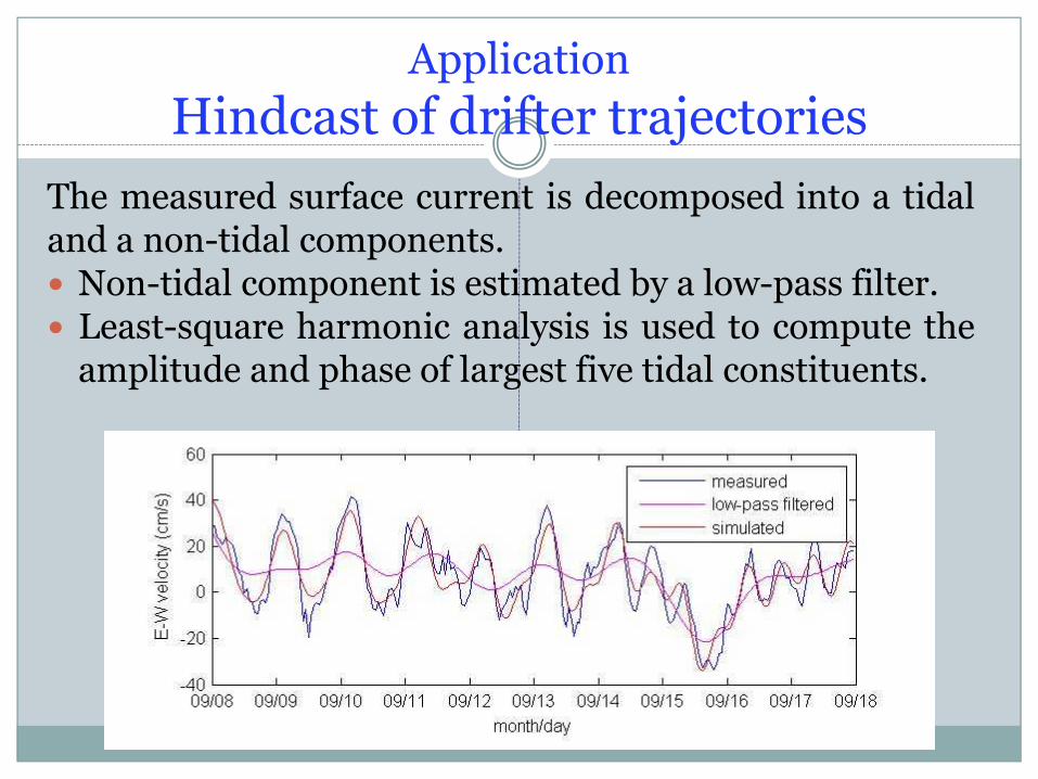
ApplicationHindcast of drifter trajectories

MethodThe drifter trajectories were divided into 24-hour segments overlapped by 12 hours, which resulted in a total 32 independent sample tracks within the study area.The measured surface current is decomposed into a tidal and a non-tidal components.Non-tidal component is estimated by a low-pass filter.Least-square harmonic analysis is used to compute theamplitude and phase of largest five tidal constituents.The composition of the low-pass filtered current and tidal current was used to make 24-hour trajectory hindcasting.

ApplicationHindcast of drifter trajectories

The measured surface current is decomposed into a tidaland a non-tidal components.

Non-tidal component is estimated by a low-pass filter.Least-square harmonic analysis is used to compute theamplitude and phase of largest five tidal constituents.

Comparisons of predicted and drifter trajectories

The drifter trajectory represented by the black line and the predicted is colored redThe surface velocity field at each time step is shown.

Separations between predicted and real locations

The mean separation increases with time elapsed until ~20km where it levels off.Separation fast increases at some specific locations.

Discussions on separationThe separation is highly dependent on environmental conditions.The separation is highly dependent on environmental conditions.In this study, the complicated flow structure was observed due tothe strong Kuroshio (~1m/s) interacted with the dramaticallychanged topography and the eddy transportation from Pacificocean.

After three and half years efforts, TORI had successfully installed 15 HFR systems around Taiwan. HFR mapped ocean surface currents provided the valuable information for the understanding of ocean environment, especially for the extreme conditions such as the strong NE monsoon period and typhoon events.

The ocean surface currents derived by HFR had been validated by the deployment of drifters and the results were comparable to those of previous studies, which confirmed the reliability of TORI’s HFR systems.

Some applications had been demonstrated, although detailed investigations need to be done before solid conclusions can be made.

Conclusions

Real time flow field shows onlinehttp://med.tori.org.tw/CODAR/

TORI welcome any kind of cooperation

Time-Series data

Range-Series

Cross Spectra File(CS)

Cross Spectra Short Time File(CSS)

Radial Vector file

Total file

FFT

FFT

Spectral to Radial

Flow diagram of data processingEcho Strength VS. Range

1024 sample @ 1Hz

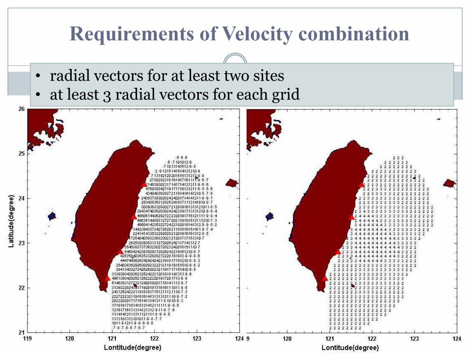
Requirements of Velocity combination

• radial vectors for at least two sites• at least 3 radial vectors for each grid

Coverage of radial velocity in time and space

Generally, valid sample decreases with increasing range, except a low value at ~100km (left figure).A periodic range fluctuation in time was found (bottom figure).

U & V OQ021N_A

The drifter experienced a small scale eddy at the afternoon of July 3, which flow field can not be reasonably resolved due to the limitation of spatial resolution of long range CODAR.

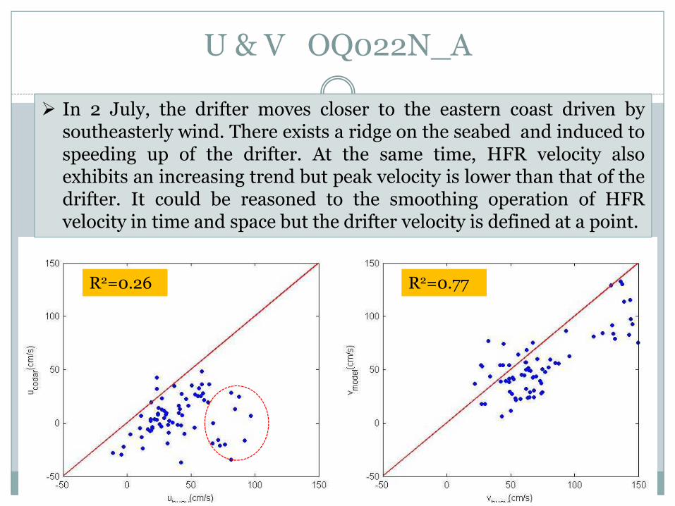
U & V OQ022N_A

R2=0.77R2=0.26

In 2 July, the drifter moves closer to the eastern coast driven bysoutheasterly wind. There exists a ridge on the seabed and induced tospeeding up of the drifter. At the same time, HFR velocity alsoexhibits an increasing trend but peak velocity is lower than that of thedrifter. It could be reasoned to the smoothing operation of HFRvelocity in time and space but the drifter velocity is defined at a point.