WEMo (Wave Exposure Model)

User Manual

Version 3.0 November 2006

WEMo

(Wave Exposure Model)

for use in Ecological Forecasting

Mark S. Fonseca and Amit Malhotra

Applied Ecology and Restoration Research Branch

NOAA, National Ocean Service Center for Coastal Fisheries and Habitat Research (CCFHR)

Beaufort, North Carolina, 28516

mark.fonseca@noaa.gov; amit.malhotra@noaa.gov

Version 3.0 / November 20th, 2006

2

TABLE OF CONTENTS

WEMo Overview ….….………………………………………………..……..……... 5

System Requirements …………………………………………………...……..…… 7

WEMo Installation ……………..………………………………………………..….. 7 Files Installed……………………………………………………………….……7

Project Composition …………………………………………………………….…...8

Getting Started Interface Description ……………………………………………..……....……..9 Toolbar Description……………………………………..……………….….. ….9 WEMo Mode………………………………………………………………….…10 Settings …………………..………………………………………….……….…. 11 Create a project file……………………………………………………………...16 Opening a project file ……………………………………………………….…..23 Adding Point Dataset …………………………………………………..……… 24 Running WEMo ……..……………………………………………………….….26 Output files (RWE)………………………………………………………………27 Additional Functionality

Projection properties ………………………………………… …………..……28 Removing project …………………………………………… …………………28 Deleting project ………………………………………………… ……………...28 Save project ………………………………………………… ………………….28 Change dataset ……………………………………………… …………………28 Remove dataset …………………………………………… ……………….......28 Identify………. ………………………………………….……………………....29 Help……………………………………………………….………………….…..29 REI Mode Utilities Analyze Wind Data…….………………………………………………………..29 Wind Data………………………………………………………………….…….31 Data Requirements ………………………………………………………….………31 Shoreline Dataset………………………………………….………………………...32 Bathymetry Dataset…………………………………….………………………….. 32 Wind Data (REI)………………………………………………………………….....33 Sample Dataset…………………………………………………….…………...........35

Finding & Building Data …………………………………………………………..35

Appendix A (REI Mode)………………………………………….…..………….....46

Appendix B………………………………………………………...……………….......52

3

Appendix C………………………………………………………...……………….....56

Contact Information………………………………………..….……………….......65

References…………………………………………………..…..………………..........66

4

WEMo 3.0 Overview The Wave Exposure Model 3.0 (WEMo 3.0) was designed to bridge the gap between ecologists and managers on one hand, and physical hydrologists on the other. Generally, the physical context is poorly represented in ecological field studies largely because there are few simple-to-use, inexpensive, parsimonious tools to provide objective information that do not require extensive advanced physical models. Wind waves, particularly those associated with storm events, are unpredictable and sometimes pose dangerous situations under which to collect empirical information, whereas in contrast tidal currents are more readily addressed because of their predictable and systematic nature. Therefore, we have attempted to create a process that allows the uninitiated ecologist, biologist, resource manager, etc., to add a tool to their analytical toolbox that accurately represents the effect of exposure to wind waves for their particular study situation. The most essential part of running WEMo is assembling the input data. Therefore, the user must make some judgments as to what kind of data are appropriate to use. Finer resolution datasets (spatially as well as temporally) potentially increase the precision of the output but also dramatically increase the processing time. WEMo was modified in this version (WEMo 3.0) to calculate wave height and derived wave energy called Representative Wave Energy (RWE) along with the relative index calculated in older WEMo versions (called Relative Exposure Index; REI). Selection of the mode depends on the project requirement, geographical area for the study and time scale used in the study. Each mode is discussed separately. RWE Mode Coastal managers are often required to estimate wave energy in coastal regions or in inland waters from local wind information. This entails the computation of wave propagation in coastal regions with shallow waters taking into account the effects of wind and local bathymetry. WEMo is modified to essentially carry out such computations as a numerical one-dimensional model. Representative wave energy (RWE) computed by WEMo is based on linear wave theory and ray tracing technique. It represents the total wave energy in one wavelength per unit wave crest width. RWE units are J/m or kg/m/s2. (USACOE, Shore Protection Manual, Vol. 1) WEMo computes the wave height for RWE in a monochromatic approach, i.e. along each ray generated by the winds in same direction. Waves generated are propagated along the fetch rays. Propagation of water waves over irregular bottom bathymetry involves processes like shoaling, refraction, diffraction and energy dissipation. In order to decrease complexity and computation time, refraction and diffraction of the waves are neglected and propagation is carried out by shoaling, wind generation and dissipation over downwind distance over water (fetch). The final output is the combined effect of wind generation, shoaling and dissipation due to wave breaking and a fetch-weighting process to account for shoreline irregularities. Fetch is defined as the distance from the site to land along a given compass heading. Fetch value can be adjusted in WEMo, 10km is the default value. Effective fetch was computed by measuring along a user-selected set of rays radiating out from either side of the ith compass heading at equal degree increments (total number of rays ranges between 16 and 56, depending on the judgment of the User in the need

5

to capture shoreline shape; uncomplicated, linear shorelines can probably be accurately assessed using the lowest number of rays while highly crenulated shorelines with complicated intervening bathymetry should use the maximum number of rays). Effective fetch is then calculated by summing the product of fetch x cosine of the angle of departure from the ith heading over each of n number of lines and dividing by the sum of the cosine of all angles. This weighting of multiple fetch measures for each ray heading helps account for irregularities in shoreline geometry that could misrepresent the potential of wind wave development from a given direction. REI Mode REI mode does not compute wave energy. In contrast, an internally consistent relative index value calculated for a site provides a context for evaluating how exposed a site is to wind-generated waves in comparison to any other site. The higher the REI value at a site implies higher wave energy will be experienced at that site, hence REI values are used for comparing among two sites under seemingly like conditions. For those working in fairly uncomplicated geomorphologic settings and needing only a quick approximation, REI mode will give values that behave quite similar to RWE, but at a fraction of the computational cost. To compute the REI using WEMo, each of the major eight compass headings, wind speed, frequency of wind from that direction and fetch are combined to produce a relative exposure index. Fetch is defined as the distance from the site to land along a given compass heading. Fetch longer than 10km were clipped at 10 km as this was considered to be a sufficient distance to generate a maximum wave height effect following empirical experimentation with the USACOE Automated Coastal Engineering System software (version 1.07). Although the fetch may be adjusted in WEMo, 10km is recommended. Effective fetch was computed by measuring along 4 lines radiating out from either side of the ith compass heading at increments of 11.25 degrees, including the ith heading. Effective fetch is then calculated by summing the product of fetch x cosine of the angle of departure from the ith heading over each of nine lines and dividing by the sum of the cosine of all angles. This weighting of multiple fetch measures for each compass heading helps account for irregularities in shoreline geometry that could misrepresent the potential of wind wave development from a given compass heading. A Note About Tides The reader will see that throughout the manual there are references to downloading bathymetry data from various sources. It is critical that the user understand the tidal reference of the data they are using; most of the sources we use in this program are set to Mean Lower Low Water (MLLW). Thus, if one wanted to assess exposure of a site to waves at high tide – especially when there is significant tidal amplitude, the user would have to manually adjust the entire bathymetry data set to account for their desired stage of the tide. As a result, the user may want to consider several runs of WEMo at different tide stages in order to account for the influence of shoals as they become submerged (and less effective at diminishing waves) with increased tide. Similar considerations should be taken for storm or El Nino effects where systematic changes in tidal elevation are anticipated.

6

System Requirements The following are the hardware requirements of WEMo 3:

• 400 MHz CPU (Recommend 1GHz or above) • 128 MB (Recommend 256 MB or above)

• 50 MB minimum free space of hard disk is need to install and run the program.

The following are the software requirements of WEMo 3: In order to install and use WEMo 3, you must have the following:

• Microsoft Windows 98/ME/XP/2000. It is recommended that you have latest service pack for each operating system

• ArcGIS 9.1 or higher version from ESRI

Note: ArcInfo or ArcEditor license is required for some steps described in creating shoreline input dataset (pg. 42).

WEMo Installation WEMo should install easily. Make sure ArcGIS 9.1 or higher version is installed on the PC where you are installing WEMo. If you have an ArcView network installation, then you’ll need to install the WEMo on the ArcView network server. Confirm that you have administrative privileges. If you do not you will have to contact your system administrator to install WEMo. Insert the WEMo installation CD into the drive and double CLICK on file WEMo.msi. Follow the instructions provided by the setup program to install the WEMo. WEMo will be installed in a directory, which you have selected and that will become the application path. Files Installed Following important files are installed by WEMo installation in program folder. WEMo.exe C:\Program Files\WEMo3.0 WEMo_V3.pdf C:\Program Files\WEMo3.0\Help WEMo 3_install.doc C:\Program Files\WEMo3.0\Help

7

Project Composition WEMo organizes data into projects. Project files contain the bathymetry grid, shoreline coverage, processed wind data file and zero or more point datasets. Project file structure is defined in the diagram below.

Project Structure

Project

Bathymetry Shoreline Wind data Input Input Input Input/create

1..111

Density Plot TableOutput 1..Output 1.. 1..

Point shapefileOutput

Point grid

WEMo 3 projects have a unique extension of *.wpro_RWE or *.wpro_REI based on the running mode of WEMo. It is an ASCII format file storing the information about various datasets. Project files may have one and only one shoreline coverage, bathymetry grid and processed wind data file but any number of point datasets associated with them. These are the four required datasets needed for running the model. Project files may be stored anywhere and can have any name recognized by Microsoft Windows. They can also be created and deleted using WEMo 3.

8

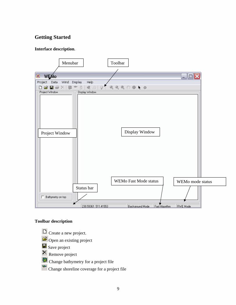
Getting Started Interface description.

Menubar Toolbar

Display Window Project Window

Toolbar description

Create a new project.

Open an existing project Save project Remove project

Change bathymetry for a project file

Change shoreline coverage for a project file

Status bar WEMo Fast Mode status WEMo mode status

9

Change wind data for a project file

Create point dataset. Add external point dataset

Run Zoom in Zoom out Zoom select Pan

Full extent Identify

WEMo Mode As mentioned previously, WEMo 3 can run in two modes, Representative Wave Energy (RWE) mode and Relative Exposure Index (REI) mode. RWE mode is a physical model mode where WEMo calculates the average wave energy flux per unit wave crest width. According to U.S. Army Corps of Engineer’s Shore Protection Manual 1977, wave energy flux is the rate at which energy is transmitted in the direction of wave propagation across a vertical plane perpendicular to the direction of wave advance and extending down the entire depth (unit W/m or kg-m /s3). REI mode is a non-physical relative mode to assess the amount of energy reaching a location. REI values are compared spatially or temporally to provide a context for evaluating how exposed a site is to wind-generated waves in comparison to any other site. REI approaches a unit-less dimensionless quantity in flat, non-varying landscapes; as such we do not ascribe any units to WEMo. The higher the REI value at a site implies higher wave energy will be experienced at that site. REI is a very parsimonious factor in simple landscapes and has the benefit of faster calculation. WEMo mode can be selected based on the project requirement and data analysis method chosen. WEMo mode can be accessed from menu bar Data WEMo Mode. WEMo always starts in RWE mode and should be changed every time application is started to access REI mode.

10

Settings Settings for WEMo can be accessed from menu bar Data Change Settings. Settings should be checked after installation of WEMo and before running each session. Settings options are different depending on the WEMo mode. RWE Mode The window’s first tab ‘General’:

1. Select the path for storing WEMo project; default path is the application path. 2. Type the name of WEMo project file, default is “WEMo_Proj”. 3. Choose the number of rays created for each site. 4. Check to use faster clipping algorithm. Checking this option means that the

bathymetry grid used for processing should reach zero water depth as near to the shoreline as possible or the bathymetry grid should be clipped with accurate shoreline vectors to set the location of the shoreline in the bathymetry grid itself (also, see “A Note About Tides” section, above). Creating the Clipped grid requires ESRI ArcMap and Spatial Analyst extension. Unchecking this option makes WEMo 3 run slower and can only process 500 points or less at a time. Points can be divided into smaller group and processed separately.

5. Check box ‘Remove refresh capability and run WEMo in background’ to allow WEMo running in the background without the graphic display and interference. This option makes WEMo run faster.

11

Setting window’s second tab “Parameters” set physical constants to run the model.

1. Select the maximum fetch limit in meters. Fetch is defined as the distance from the site to the first encountered land along a given compass heading. The default fetch set in WEMo is 10,000 m, a value based on an empirical assessment of the distance to fully develop a wave using linear wave theory (Automated Coastal Engineering System, US Army Corps of Engineers v1.07).

2. The Fetch Length Segment selection defines how far out from the point of interest that WEMo uses the maximum resolution of the bathymetry grid to conduct interrogations of the effect of water depth (i.e., if your bathymetry data set had 6 m resolution between depth measurements, WEMo would assess the effect of bathymetry every 6 m). The default value is set at 1000 m. Make sure this value is smaller than maximum fetch selected.

3. Beyond the distance selected in (2), WEMo will use the value set in the Bathymetry Interrogation Distance Box for the spacing interval at which bathymetry is interrogated; the default spacing is 100 m. We give the option of making the spacing coarser beyond the Fetch Length Segment to save on computing resources as the influence in bathymetric changes at these distances from the point of interest have comparatively little effect on the overall

12

computations of exposure. We do not recommend ever attempting to use a resolution (spacing) finer than that of the bathymetry grid itself.

4. The next three parameters are set for determining wave breaking constants and should only be changed after careful analysis.

Alpha in Goda’s formula is a constant set at 0.17 default value. Sensitivity eps is used to get estimation accuracy in calculating model values. Default value is set at 1 in 1000. Beach slope is set at 1.909 degrees equivalent to 1/30; this is a very shallow

slope; note that the angle of repose of most sand is closer to 1/3 which would be more appropriate for channel margins.

To set the default values check ‘Set default settings’ and all values returned to the default.

13

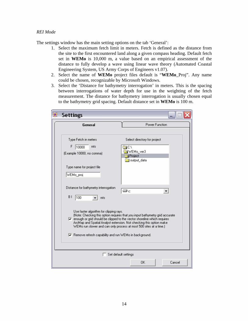
REI Mode The settings window has the main setting options on the tab ‘General’:

1. Select the maximum fetch limit in meters. Fetch is defined as the distance from the site to the first encountered land along a given compass heading. Default fetch set in WEMo is 10,000 m, a value based on an empirical assessment of the distance to fully develop a wave using linear wave theory (Automated Coastal Engineering System, US Army Corps of Engineers v1.07).

2. Select the name of WEMo project files default is “WEMo_Proj”. Any name could be chosen, recognizable by Microsoft Windows.

3. Select the ‘Distance for bathymetry interrogation’ in meters. This is the spacing between interrogations of water depth for use in the weighting of the fetch measurement. The distance for bathymetry interrogation is usually chosen equal to the bathymetry grid spacing. Default distance set in WEMo is 100 m.

14

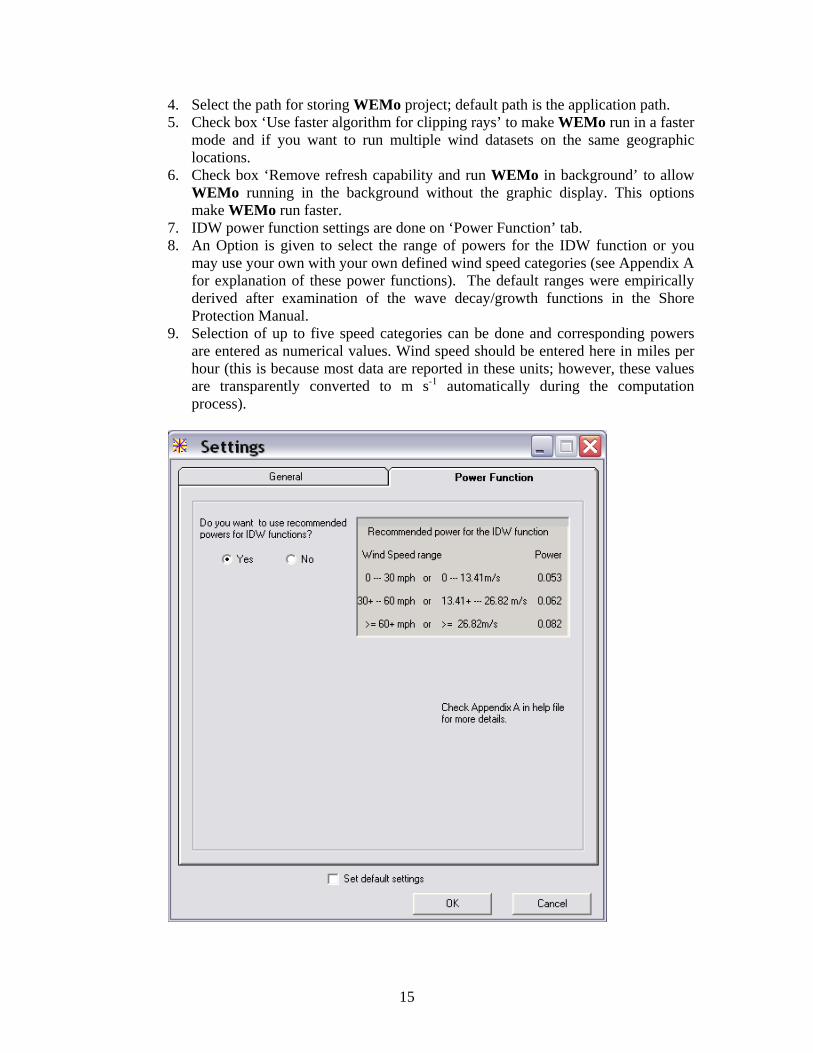
4. Select the path for storing WEMo project; default path is the application path. 5. Check box ‘Use faster algorithm for clipping rays’ to make WEMo run in a faster

mode and if you want to run multiple wind datasets on the same geographic locations.

6. Check box ‘Remove refresh capability and run WEMo in background’ to allow WEMo running in the background without the graphic display. This options make WEMo run faster.

7. IDW power function settings are done on ‘Power Function’ tab. 8. An Option is given to select the range of powers for the IDW function or you

may use your own with your own defined wind speed categories (see Appendix A for explanation of these power functions). The default ranges were empirically derived after examination of the wave decay/growth functions in the Shore Protection Manual.

9. Selection of up to five speed categories can be done and corresponding powers are entered as numerical values. Wind speed should be entered here in miles per hour (this is because most data are reported in these units; however, these values are transparently converted to m s-1 automatically during the computation process).

15

Power for IDW function represents the effect of fetch on the site. The higher the power value, the lower the effect of fetch on the REI values. Lower power represents more of an effect of distance. For more details check Appendix A. CLICKing OK will change the settings and they will remain same even after you close the application, so you don’t have to change them every time. Checking the ‘Default’ button changes the current settings to default. Note – Settings should always be checked after loading or creating a Project to ensure that

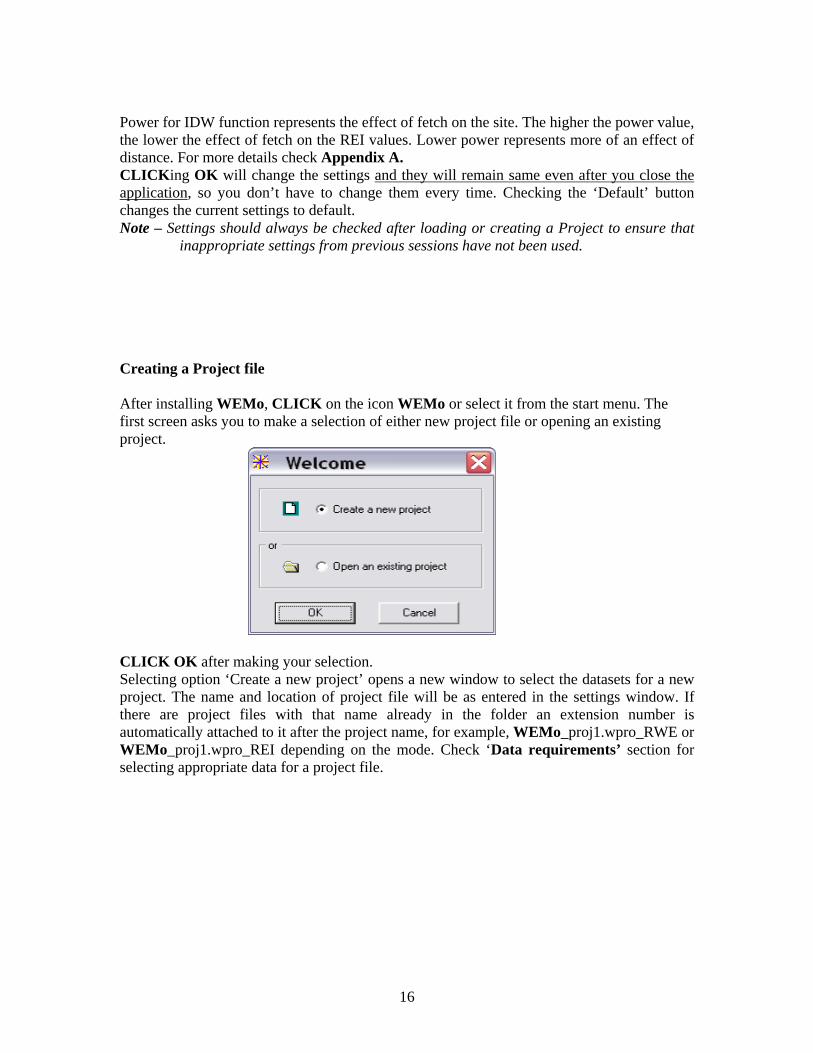
inappropriate settings from previous sessions have not been used. Creating a Project file After installing WEMo, CLICK on the icon WEMo or select it from the start menu. The first screen asks you to make a selection of either new project file or opening an existing project.

CLICK OK after making your selection. Selecting option ‘Create a new project’ opens a new window to select the datasets for a new project. The name and location of project file will be as entered in the settings window. If there are project files with that name already in the folder an extension number is automatically attached to it after the project name, for example, WEMo_proj1.wpro_RWE or WEMo_proj1.wpro_REI depending on the mode. Check ‘Data requirements’ section for selecting appropriate data for a project file.

16

Bathymetry grid - CLICK on the Browse button in ‘Add bathymetry grid’ section to select a bathymetry data layer. The appropriate grid is selected from the file browser. If you can’t see your folder or directory, you have to add it using the Connection button. To see the appropriate format of a grid accepted by WEMo check ‘Data requirement section’. After selecting bathymetry please select the appropriate units that were used in this data for the depth (m, ft or cm). Check the box ‘Bathymetry Positive’ if depth in the grid is represented by positive numbers instead of negative (i.e., if the depth is measured from the seafloor as opposed to from the water surface). When the faster algorithm option is checked in the settings windows the bathymetry grid should reach zero water depth as near to the shoreline as possible or the bathymetry grid should be clipped with accurate shoreline vectors to set the location of the shoreline in the bathymetry grid itself (also, see “A Note About Tides” section, above).

17

Connection button

Shoreline coverage - CLICK on ‘Browse’ button in ‘Add shoreline coverage’ section in ‘New project’ window to select a shoreline. The appropriate grids are selected from the file browser. If you can’t see your folder or directory, you have to add it using the ‘Connection’ button. Either shapefile or Arc coverage formats are allowed. Both shoreline coverage and bathymetry grid must be projected in same projected coordinate system like UTM or state planes and not in Geographic coordinate system. Wind data – For REI mode there are two options for selecting wind data for a project, either you can create a new wind data file or you can attach a previously created wind data file by CLICKing the appropriate option button. If you CLICK the ‘Text file’ option, you have to select an already created Wind data using the ‘Browse’ button in ‘Wind data’ section. Once selected the REI wind file will have extension *.Wind_REI. This file is a product of the ‘Analyze Wind Data’ option in the Wind menu. The default folder is the application path. If your selection is ‘manual’ a new form opens where you can enter the wind data; i.e. wind speed and wind frequency for eight compass heading directions, station name from where data was collected and start and end time for the data analyzed. After entering the data you could save the wind data file for future purposes. If data are not saved in a text file, ‘memory’ will be written in front of the wind data in the Project window and the data will NOT be saved when the session ends.

18

For RWE mode all data are created using ‘Analyze Wind Data…’ command accessed from Wind menu. Wind files are directly downloaded from National Data Buoy Center (NDBC) website for select stations from the list. Select the start year, month, day, and hour to choose the starting time for analyzing wind data. You have the option of selecting time to the nearest hour as temporal resolution. Similarly, select the ending year, month, day and

19

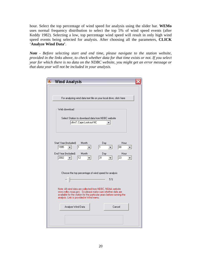
hour. Select the top percentage of wind speed for analysis using the slider bar. WEMo uses normal frequency distribution to select the top 5% of wind speed events (after Keddy 1982). Selecting a low, top percentage wind speed will result in only high wind speed events being selected for analysis. After choosing all the parameters, CLICK ‘Analyze Wind Data’. Note - Before selecting start and end time, please navigate to the station website, provided in the links above, to check whether data for that time exists or not. If you select year for which there is no data on the NDBC website, you might get an error message or that data year will not be included in your analysis.

20

In case no station is found in the downloadable NDBC list for your area, WEMo can process text files containing wind data in certain format. Text file could be space, tab or Comma delimited and should be in NDBC wind data file format. NDBC file format is described below:

• All fields are divided into individual columns separated by delimiters. • Wind speed is in meter per second. • Wind direction is the direction the wind is coming from in degrees in clockwise from

true north. • Data should be at least every hour and can be up to 1minute temporal resolution.

Example of NDBC format: YY MM DD hh WD WSPD GST 95 01 01 00 154 9.2 10.1 Other formats of wind text files should be manipulated in MS Excel or other software to match NDBC format before processing. Import of the wind data from the text file should always start importing from the row where headers are located. Unwanted data entries should be clipped before importing either by selective highlighting or simple trimming and saving before importing.

21

After selecting all the parameters CLICK OK and WEMo will ask you to type in the station name for metadata purposes along with start and end dates and top percentage of wind speed, similar to REI mode.

Note - Use only numeric values otherwise an error message will be generated. Note - Always save wind data associated with a current project otherwise the wrong wind

data may be used for processing (i.e. data from a previous session). Whenever you see a temporary file with project wind data in the project window, create a different project or add a new wind data file.

Note – When manually entering wind speed, you may select different units; the program checks your selection and transparently converts it to m s-1.

22

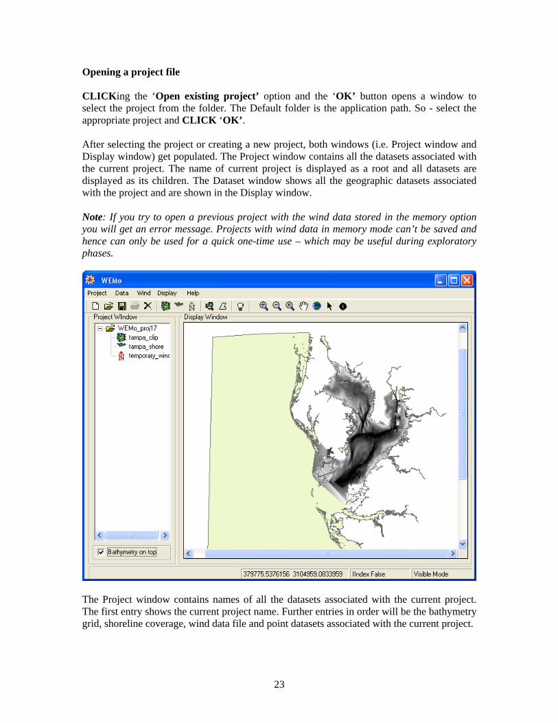
Opening a project file CLICKing the ‘Open existing project’ option and the ‘OK’ button opens a window to select the project from the folder. The Default folder is the application path. So - select the appropriate project and CLICK ‘OK’. After selecting the project or creating a new project, both windows (i.e. Project window and Display window) get populated. The Project window contains all the datasets associated with the current project. The name of current project is displayed as a root and all datasets are displayed as its children. The Dataset window shows all the geographic datasets associated with the project and are shown in the Display window. Note: If you try to open a previous project with the wind data stored in the memory option you will get an error message. Projects with wind data in memory mode can’t be saved and hence can only be used for a quick one-time use – which may be useful during exploratory phases.

The Project window contains names of all the datasets associated with the current project. The first entry shows the current project name. Further entries in order will be the bathymetry grid, shoreline coverage, wind data file and point datasets associated with the current project.

23

Adding point datasets Point datasets may be added in three ways for a current project. Note: Point datasets may only be added after you have a current project. Note: All points selected for sites MUST lie OVER the shoreline and bathymetry datasets,

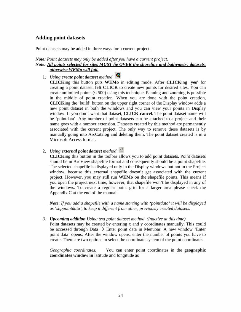
otherwise WEMo will fail. 1. Using create point dataset method.

CLICKing this button puts WEMo in editing mode. After CLICKing ‘yes’ for creating a point dataset, left CLICK to create new points for desired sites. You can create unlimited points (< 500) using this technique. Panning and zooming is possible in the middle of point creation. When you are done with the point creation, CLICKing the ’build’ button on the upper right corner of the Display window adds a new point dataset in both the windows and you can view your points in Display window. If you don’t want that dataset, CLICK cancel. The point dataset name will be ‘pointdata’. Any number of point datasets can be attached to a project and their name goes with a number extension. Datasets created by this method are permanently associated with the current project. The only way to remove these datasets is by manually going into ArcCatalog and deleting them. The point dataset created is in a Microsoft Access format.

2. Using external point dataset method. CLICKing this button in the toolbar allows you to add point datasets. Point datasets should be in ArcView shapefile format and consequently should be a point shapefile. The selected shapefile is displayed only in the Display windows but not in the Project window, because this external shapefile doesn’t get associated with the current project. However, you may still run WEMo on the shapefile points. This means if you open the project next time, however, that shapefile won’t be displayed in any of the windows. To create a regular point grid for a larger area please check the Appendix C at the end of the manual. Note: If you add a shapefile with a name starting with ‘pointdata’ it will be displayed as ‘shppointdata’, to keep it different from other, previously created datasets.

3. Upcoming addition Using text point dataset method. (Inactive at this time) Point datasets may be created by entering x and y coordinates manually. This could be accessed through Data Enter point data in Menubar. A new window ‘Enter point data’ opens. After the window opens, enter the number of points you have to create. There are two options to select the coordinate system of the point coordinates. Geographic coordinates: You can enter point coordinates in the geographic coordinates window in latitude and longitude as

24

decimal degrees. You can also select the datum for your point coordinates from three choices of NAD1983, NAD 1927 and WGS 1984. The points are then converted into the current project datasets coordinate system, which could be either a geographic or a projected coordinate system. The point could also be entered by CLICKing the ‘next’ button. You could go back to previous points and make changes by CLICKing the ‘previous’ button. CLICKing on the ‘final’ button (‘next’ changes to ‘final’ after entry of the last of the points) creates the new dataset or you could CLICK ‘cancel’ to end without creating points. The point dataset created is in a Microsoft Access format.

UTM coordinates: However, you may also enter point coordinates in the UTM coordinate system. Select the zone of UTM for your point coordinates (if you need reference for selecting UTM please check the website referred in the ‘Finding data’ section). You also have to select the datum for the UTM coordinates.

25

The newly created point dataset is added to all three of the WEMo windows unlike the externally added dataset. The default name assigned to the dataset would be ‘pointdata_ext’. If there is already a point dataset with this name an extension is added at the end of dataset name e.g. ‘pointdata_ext1’. The point dataset created is in a Microsoft Access format. Note: This functionality is not fully functional yet.

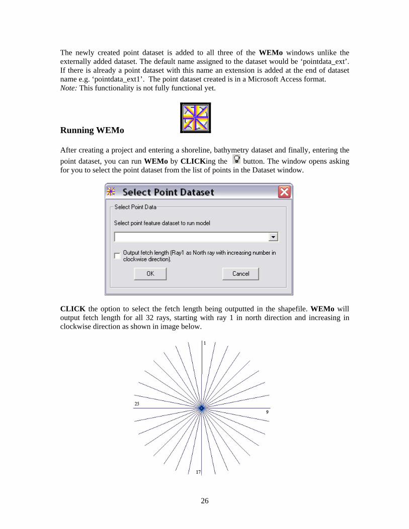
Running WEMo After creating a project and entering a shoreline, bathymetry dataset and finally, entering the point dataset, you can run WEMo by CLICKing the button. The window opens asking for you to select the point dataset from the list of points in the Dataset window.

CLICK the option to select the fetch length being outputted in the shapefile. WEMo will output fetch length for all 32 rays, starting with ray 1 in north direction and increasing in clockwise direction as shown in image below.

26

After selecting a point dataset and CLICKing the OK button, WEMo runs for each point in the selected dataset successively. In the point dataset, a new field is created named ‘RWE’ or ‘REI’ depending on the WEMo mode. Index values could be viewed using the Identify tool in the toolbar for each point, or opening the dataset attribute table in either ArcMap or ArcCatalog. Attribute tables could be exported to MS Excel file or dbase or could be exported as a shapefile from the geodatabase. If an external shapefile is selected for running WEMo, a new field is created in that shapefile with calculated REI values. Note: Running WEMo is a CPU intensive task, it consumes CPU time. Also once you CLICK the ‘run’ button to start processing; you can’t stop processing unless you use Windows Task Manager to shut it down. So carefully select all the parameters before running WEMo. Output files (RWE) Many other additional files are created by WEMo in RWE mode, mostly used for debugging or later use on detailed analysis. Output files have data only for individual points and are rewritten every time a point is processed; hence it only contains data for last point processed. All these files are saved in the application folder under Project\output_data. A list of these files is mentioned below. Windarray.txt = Wind speed and frequency for individual rays. Fetcharray.txt = Fetch distance (meters) for each ray. Wave_HT_first\waveHt_first i.txt = wave height observed for the first fetch segment for the ith ray at the site. Wave heights recorded at every few meters specified in WEMo settings. Wave_depth_first\depth_first i .txt = average depth observed under the first fetch segment for the ith ray at the site. Depth recorded at every few meters specified in WEMo settings. Wave_HT_second\waveHt_second i.txt = wave height observed for the rest of fetch segment for the ith ray at the site. Wave heights recorded at every few meters equal to the resolution of bathymetry grid. Wave_depth_first\depth_second i .txt = average depth observed under rest of the fetch segment for the ith ray at the site. Depth recorded at every few meters equal to the resolution of bathymetry grid. WaveHt.txt = Final wave height in meters for individual rays for the last point processed. RWE.txt = Final RWE values for each of the rays for the last point processed.

27

Additional Functionality Projection properties The current project projection properties can be checked using this utility. This utility may be accessed through Data Projection Properties or by right CLICKing either bathymetry dataset or shoreline dataset in the Project Window.

Removing projects Projects currently loaded may be removed using the tool or using menu Project Remove project. This could also be accessed using the right CLICK on ‘Project name’ in the Project window. Deleting projects Projects may be permanently deleted using the Project Delete project. CLICKing this menu button shows the file selection window. After selecting the project, CLICK OK, as this deletes the selected project and all attached internal files (not datasets). Save projects Current projects may be saved by CLICKing Project Save project. To change the project name use ‘Save Project As’ button. New projects may be saved with different names by using ‘Save project As’ button. Change datasets Current project datasets could be changed using menu buttons or toolbar tools.

To change shoreline data use Data Change shoreline coverage or toolbar button

To change bathymetry data use Data Change bathymetry coverage or toolbar button To change wind data use Data Change wind data or toolbar button Removing datasets Datasets may be removed from the Display window and Data window by double CLICKing in the Data window.

28

Identify Spatial features may be identified using the tool. A window opens showing the attributes of the feature. The dataset may be selected for the desired feature using the drop down menu. The location of the feature is displayed in the right window.

Help Help may be accessed using Help contents. Help file is in adobe acrobat file format. REI Mode Utilities Analyze Wind Data Wind data can be analyzed directly in WEMo. Wind data are downloaded directly from National Data Buoy Center, NOAA website. National Data Buoy Center (NDBC), a part of the National Weather Service (NWS) that develops, operates, and maintains a network of buoy and C-MAN stations. NDBC provides hourly observations from a network of about 70 buoys and 60 C-MAN stations all over the US coast. All stations measure wind speed, direction, and gusts. You may analyze wind data using WEMo by CLICKing menu ‘Wind’ ‘Analyze wind data…’ to open the window as shown below.

29

Select the station closest to your site from the ‘Select Station’ option. Various stations listed in the drop box are shown below. Note - If you can’t find any station close to your site, please check NDBC website, if you find any station close to you on the website, please send us a request to add that station at the email address listed in contact information (amit.malhotra@noaa.gov). 1. clkn7, Cape Lookout, NC 2. tplm2, Thomas Point, MD 3. chlv2, Chesapeake Light, VA 4. ducn7, Duck Pier, NC 5. dsln7, Diamond Shoal, NC 6. venf1, Venice, FL

30

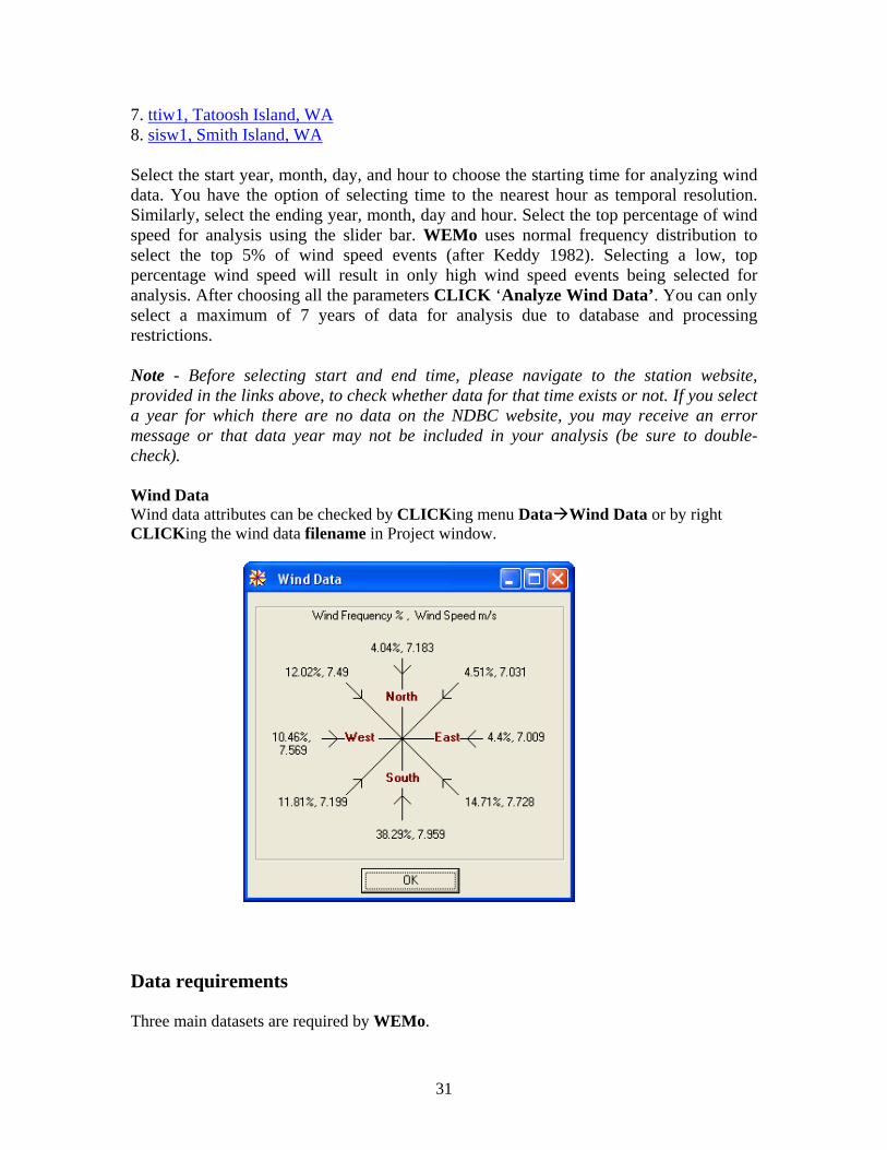
7. ttiw1, Tatoosh Island, WA 8. sisw1, Smith Island, WA Select the start year, month, day, and hour to choose the starting time for analyzing wind data. You have the option of selecting time to the nearest hour as temporal resolution. Similarly, select the ending year, month, day and hour. Select the top percentage of wind speed for analysis using the slider bar. WEMo uses normal frequency distribution to select the top 5% of wind speed events (after Keddy 1982). Selecting a low, top percentage wind speed will result in only high wind speed events being selected for analysis. After choosing all the parameters CLICK ‘Analyze Wind Data’. You can only select a maximum of 7 years of data for analysis due to database and processing restrictions. Note - Before selecting start and end time, please navigate to the station website, provided in the links above, to check whether data for that time exists or not. If you select a year for which there are no data on the NDBC website, you may receive an error message or that data year may not be included in your analysis (be sure to double-check). Wind Data Wind data attributes can be checked by CLICKing menu Data Wind Data or by right CLICKing the wind data filename in Project window.

Data requirements Three main datasets are required by WEMo.

31

Shoreline dataset The shoreline dataset is required to clip the fetch rays with the land if ‘Faster Algorithm’ is not checked. Shoreline datasets should be as detailed as possible depicting islands and proper shorelines. Requirements:

• Datasets should be either an ESRI shapefile or ArcInfo coverage format topologically clean

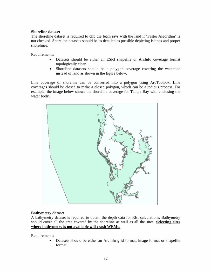
• Shoreline datasets should be a polygon coverage covering the waterside instead of land as shown in the figure below.

Line coverage of shoreline can be converted into a polygon using ArcToolbox. Line coverages should be closed to make a closed polygon, which can be a tedious process. For example, the image below shows the shoreline coverage for Tampa Bay with enclosing the water body.

Bathymetry dataset A bathymetry dataset is required to obtain the depth data for REI calculations. Bathymetry should cover all the area covered by the shoreline as well as all the sites. Selecting sites where bathymetry is not available will crash WEMo. Requirements:

• Datasets should be either an ArcInfo grid format, image format or shapefile format.

32

• Bathymetry should contain depth information in meters (negative or positive). Bathymetry in units other than meters will make it difficult to compare with other WEMo results from other users.

• Bathymetry grid spacing should be at least 100m if using a 1 ha grid size. Mismatched grid spacing creates scale mismatches with unknown consequences.

Wind data (REI mode) Wind data are required to calculate the REI values for a point. Two wind data parameters are required to run WEMo:

1. A specified percent of top hourly wind speed observation (m s-1 or mph) over the preceding years at the site from eight compass headings (default 5%),

2. The top wind (exceedance) occurrence frequency from the eight compass headings (default 5%).

Wind data may be analyzed using the WEMo analysis tool or from outside using other software. The example below shows two charts for frequency of exceedence wind and exceedance wind speed (here, top 5% of wind events by wind speed) by direction on a star chart. These

33

charts were generated using SAS.

Above: example of frequency of exceedence wind (top 5%) by direction.

Above: Example of exceedence wind speed (top 5%) by direction in m s-1.

34

Sample Dataset Sample datasets are including in the WEMo installation CD and installed along with WEMo software. These data sets have been cleaned and meet all of our previously described accuracy requirements; they may be a useful training tool as the results will not be compromised by data issues, thus allowing the user to separate training with the software from database issues. Datasets can be found in the ‘sample dataset’ folder in WEMo installation folder. Shoreline: Datasets include shoreline shapefile ‘NC_shoreline_UTM.shp’ for coastal NC area for Core and Bogue banks with UTM zone 18 NAD83 coordinate system. Bathymetry: A bathymetry grid included is for the same area with 86 m spatial resolution and UTM zone 18 NAD83 coordinate system. Wind: Also included are the processed wind data files; one each for RWE and REI mode ‘wind_nc.Wind_RWE’ and ‘wind_nc.Wind_REI’. Wind data are from the NDBC station CLKN7 at Cape Lookout, NC processed for year including 2001 to 2004 using the exceedance (top 5%) wind speeds. Finding & Building data Shoreline datasets may be found at NOAA website or USGS websites. These sites have a large collection of shoreline datasets for estuaries and bays. Bathymetry may be created using NOAA NGDS bathymetry sounding available at following website: http://www.ngdc.noaa.gov/ Website for UTM zones: http://www.dmap.co.uk/utmworld.htm Wind data may be obtained from NOAA National data buoy center website: http://www.ndbc.noaa.gov/ Another wind data website from NOAA is: http://co-ops.nos.noaa.gov/co-ops.html If wind data are not available for your particular site, data from other, nearby sites could be used for analysis if you are satisfied with its veracity. Bathymetry A bathymetry dataset is required to get the depth data for REI calculations. Bathymetry should cover all the area covered by shoreline as well as all the sites. Selecting sites where bathymetry is not available will crash WEMo or not return an REI value.

35

Bathymetry may be created using NOAA NGDC bathymetry sounding CDs available from NGDC website for a nominal charge. The website for obtaining the CDs is: http://www.ngdc.noaa.gov/mgg/fliers/01mgg05.html The CD contains Coastal Relief Models, which are topographic-bathymetric relief models that integrate land and seafloor elevations by assembling a gridded database that merges the US Geological Survey 3-arc-second DEMs with a vast compilation of hydrographic soundings collected by the National Ocean Service and various academic institutions. Eight CD-ROMs are currently available covering the US East, Gulf, and West Coasts. Steps for creating bathymetry from the Coastal Relief Model CDs

1. Install the CD obtained from NGDC by navigating to setup/Windows folder and CLICKing setup.exe. Follow on-screen instructions to install.

2. To extract a bathymetry data, you have to install the CD volume separately.

3. From the start menu navigate to Programs-> GEODAS-> Coastal Relief Model. This

will launch your browser.

4. CLICK on Design-a-Grid button in the webpage and save the grid by assigning

some appropriate name in a designated folder. 5. After saving the grid, download complete windows appear. CLICK on the ‘open

button’ to start Design-a-Grid.

36

6. When using Design-a-Grid, you must choose the database(s) you wish to use in creating your grid. The Grid Database Dialog (below) allows you to choose from among all installed GEODAS Grid Databases. CLICK OK after selecting the grid database.

7. Design-a-Grid in Grid Translator will present a grid parameters dialog. This will give you the opportunity to enter your own grid limits. Other grid parameters can be entered or changed for your output grid.

37

8. Choose the file options for your output grid. Use the Grid Options Dialog to determine format, byte swapping, header, delimiter, etc. Choose the ASCII Raster Format in Output Grid Format option and ArcInfo/ArcView Header.

38

9. CLICK OK and use this to name your output file and determine the directory you wish to save it in. The file will be saved with an .asc extension.

10. Next, open an ArcInfo workstation to generate the grid from the text file you saved.

11. To generate grid use Asciigrid ArcInfo Command.

ASCIIGRID <in_ascii_file> <out_grid> {INT | FLOAT}

Arguments

<in_ascii_file> - the ASCII file to be converted full with path. <out_grid> - the name of the grid to be created. {INT | FLOAT} - the data type of the output grid. INT - an integer grid will be created. FLOAT - a floating-point grid will be created (use floating point)

12. An Asciigrid command will generate an ArcInfo grid with projection in geographic

coordinates. You need to convert the grid projection to one you are using, for running WEMo. ArcGIS ArcInfo or ArcInfo workstation is required to project the grid to required projection.

Shoreline A shoreline dataset is required to clip the fetch with the land. Shoreline datasets should be as detailed as possible depicting islands and the actual shoreline. Line coverages of the shoreline can be converted into a polygon using the ArcToolbox. Line coverage should be closed to make a closed polygon. For e.g. the image below shows the shoreline coverage for Tampa Bay with enclosing the waterside. Shoreline Data Mining & Preparation Shoreline datasets could be found at NOAA website or USGS websites. These sites have large collection of shoreline datasets for estuaries and bays. The website to extract shoreline data from http://www.ngdc.noaa.gov/mgg/shorelines/shorelines.html

39

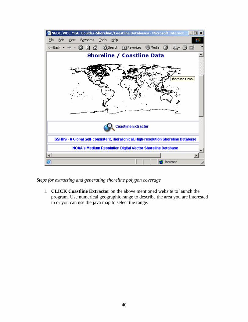
Steps for extracting and generating shoreline polygon coverage

1. CLICK Coastline Extractor on the above mentioned website to launch the program. Use numerical geographic range to describe the area you are interested in or you can use the java map to select the range.

40

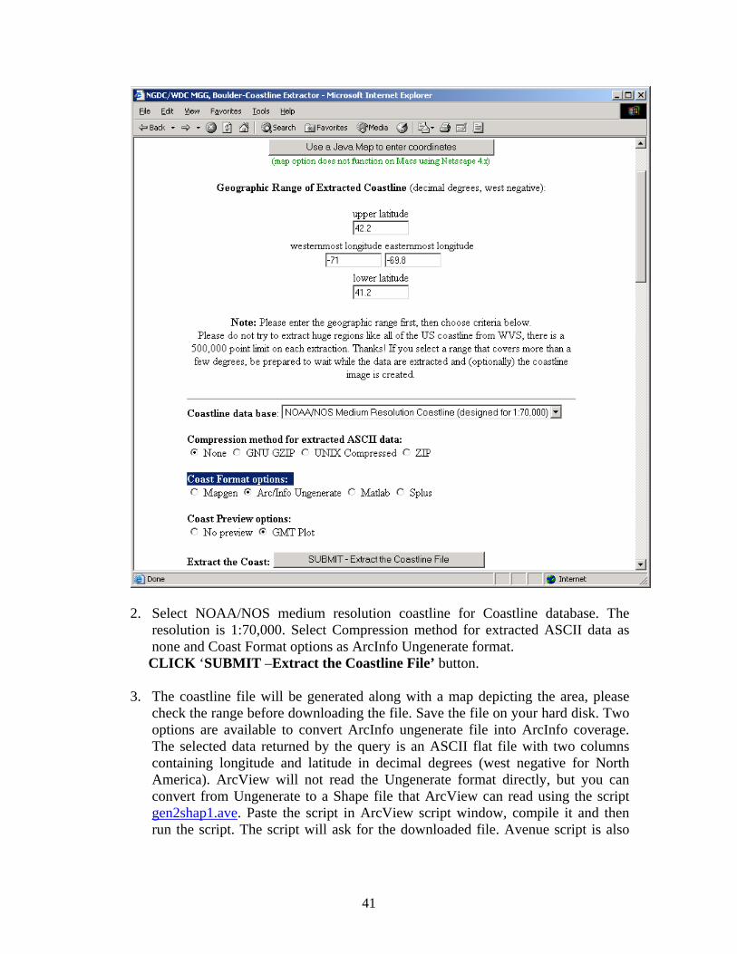
2. Select NOAA/NOS medium resolution coastline for Coastline database. The resolution is 1:70,000. Select Compression method for extracted ASCII data as none and Coast Format options as ArcInfo Ungenerate format.

CLICK ‘SUBMIT –Extract the Coastline File’ button.

3. The coastline file will be generated along with a map depicting the area, please check the range before downloading the file. Save the file on your hard disk. Two options are available to convert ArcInfo ungenerate file into ArcInfo coverage. The selected data returned by the query is an ASCII flat file with two columns containing longitude and latitude in decimal degrees (west negative for North America). ArcView will not read the Ungenerate format directly, but you can convert from Ungenerate to a Shape file that ArcView can read using the script gen2shap1.ave. Paste the script in ArcView script window, compile it and then run the script. The script will ask for the downloaded file. Avenue script is also

41

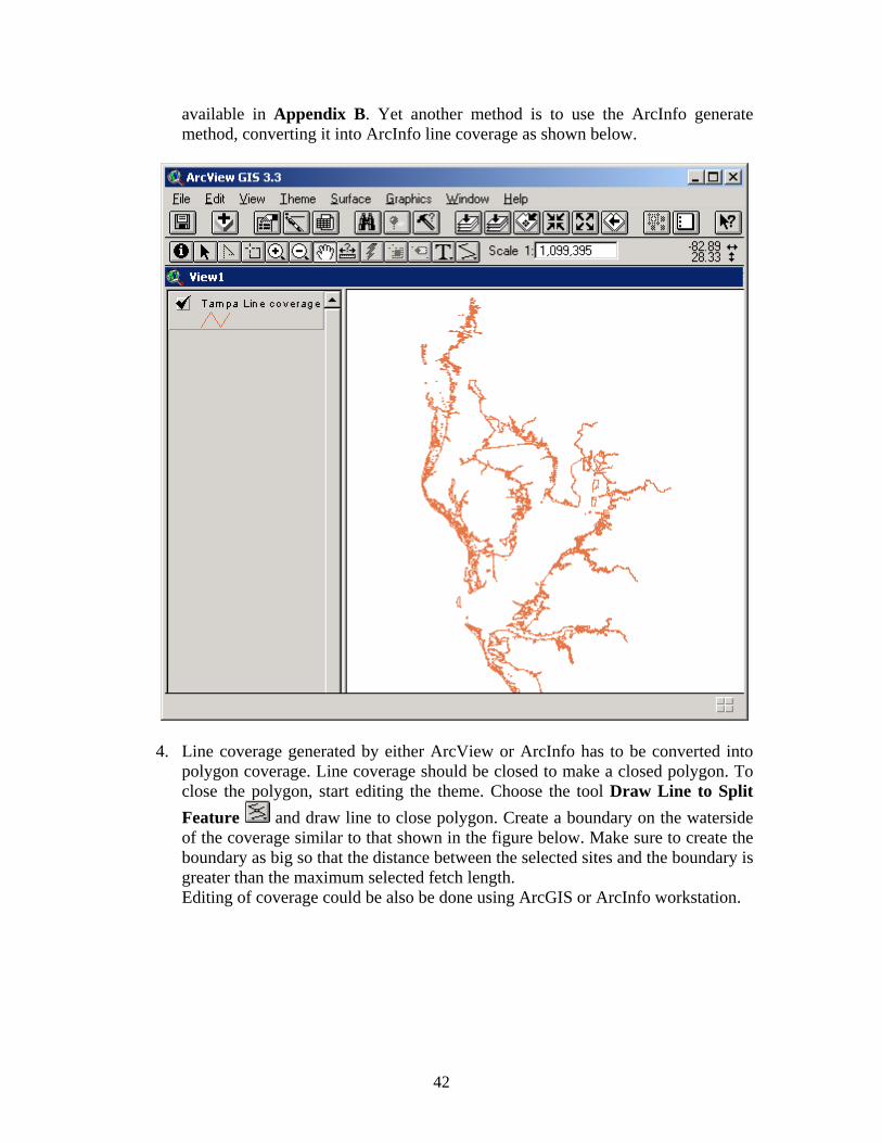
available in Appendix B. Yet another method is to use the ArcInfo generate method, converting it into ArcInfo line coverage as shown below.

4. Line coverage generated by either ArcView or ArcInfo has to be converted into polygon coverage. Line coverage should be closed to make a closed polygon. To close the polygon, start editing the theme. Choose the tool Draw Line to Split Feature and draw line to close polygon. Create a boundary on the waterside of the coverage similar to that shown in the figure below. Make sure to create the boundary as big so that the distance between the selected sites and the boundary is greater than the maximum selected fetch length. Editing of coverage could be also be done using ArcGIS or ArcInfo workstation.

42

5. After closing the line coverage it can be easily converted to polygon coverage using

ArcGIS ArcCatalog. (Note: This step requires either ArcInfo or ArcEditor license for ArcGIS) Navigate to the shapefile in ArcCatalog and right CLICK on the shapefile. From the menu select export -> shapefile to coverage. Save the ArcInfo coverage to your hard disk.

6. Right CLICK on the coverage saved above and CLICK properties. A window will

pop up as shown below. CLICK on the clean button to create the topology for the polygon coverage. The clean window will pop up. Use the default settings and CLICK OK. CLICKing Ok will generate polygon coverage with the desired topology. Note: If you don’t see proper polygon coverage, you might have gaps in your closed polygon. Try using a higher number in the ‘Clean’ window for fuzzy tolerance. If it still doesn’t generate polygon coverage closely check your polygon in line coverage for gaps.

43

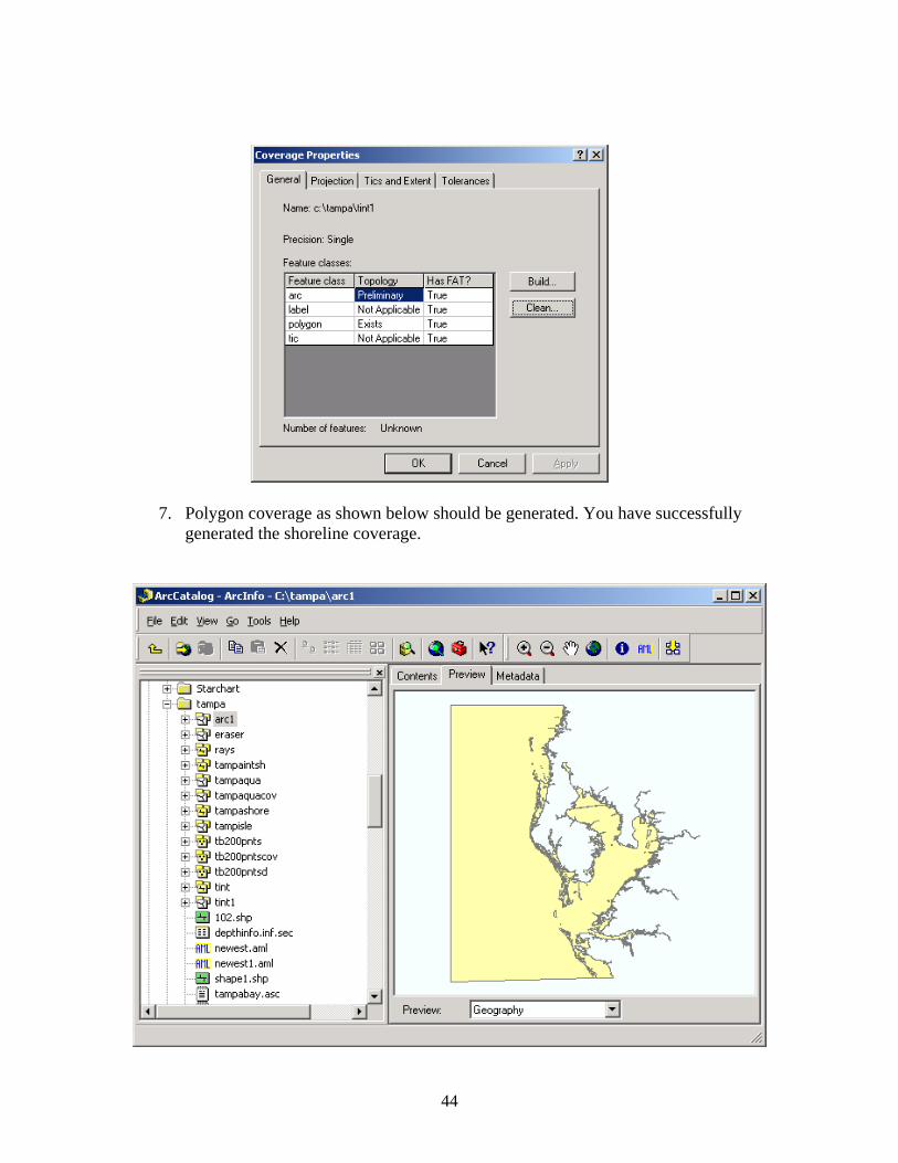
7. Polygon coverage as shown below should be generated. You have successfully generated the shoreline coverage.

44

Note: Export format files are converted to ArcInfo format using ArcInfo workstation or

ArcView 9.1 toolbox ‘Import to coverage’ option.

45

Appendix A (REI Mode)

This section provides explanation regarding the powers assigned to the Inverse Distance Weighting (IDW) function in greater detail and will focus on the numerical and other technical features. WEMo assumes wave energy generated at a site depends on the fetch, water depth and the wind speed. The IDW function calculates the mitigating effect of fetch and depth on the REI as the fetch increases and depth changes in proximity to the calculated point. The rate at which REI changes depends on the power of the IDW function.

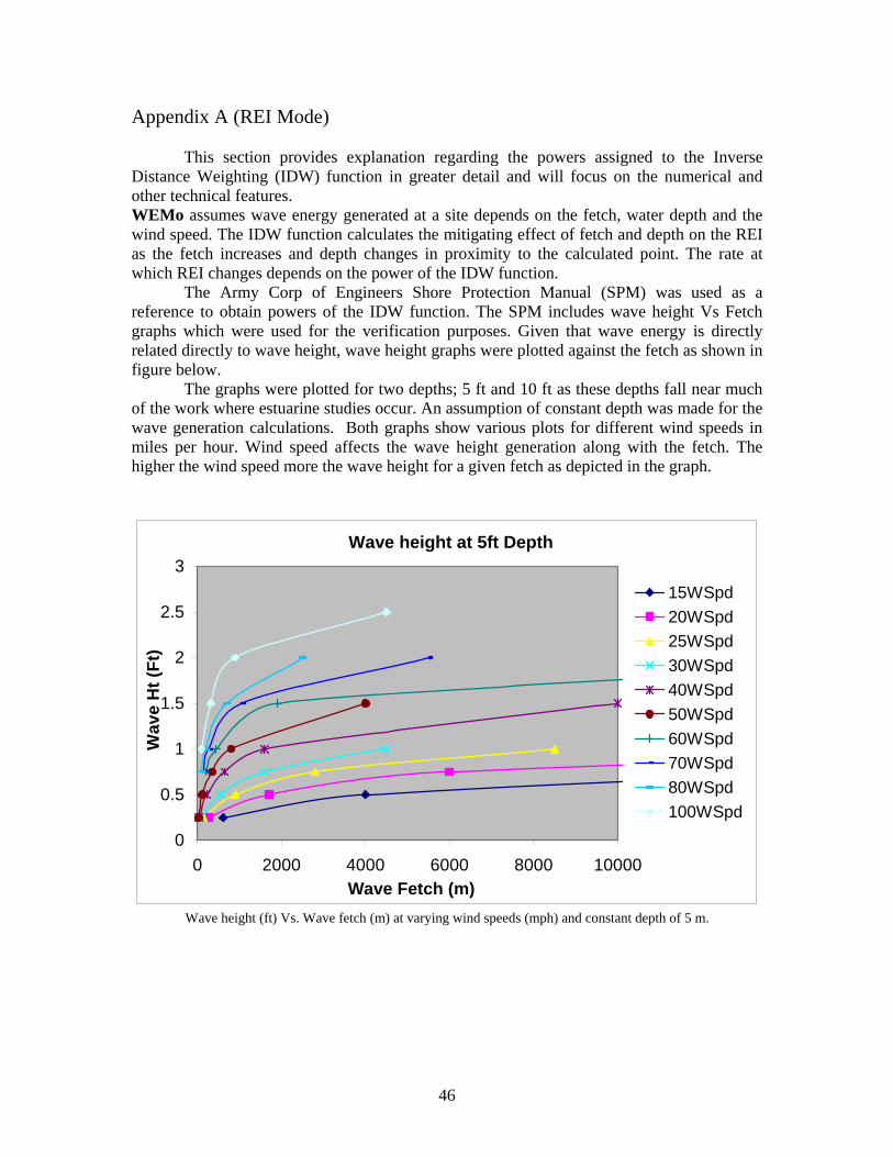
The Army Corp of Engineers Shore Protection Manual (SPM) was used as a reference to obtain powers of the IDW function. The SPM includes wave height Vs Fetch graphs which were used for the verification purposes. Given that wave energy is directly related directly to wave height, wave height graphs were plotted against the fetch as shown in figure below.

The graphs were plotted for two depths; 5 ft and 10 ft as these depths fall near much of the work where estuarine studies occur. An assumption of constant depth was made for the wave generation calculations. Both graphs show various plots for different wind speeds in miles per hour. Wind speed affects the wave height generation along with the fetch. The higher the wind speed more the wave height for a given fetch as depicted in the graph.

Wave height at 5ft Depth

0

0.5

1

1.5

2

2.5

3

0 2000 4000 6000 8000 10000Wave Fetch (m)

Wav

e H

t (Ft

)

15WSpd20WSpd25WSpd30WSpd40WSpd50WSpd60WSpd70WSpd80WSpd100WSpd

Wave height (ft) Vs. Wave fetch (m) at varying wind speeds (mph) and constant depth of 5 m.

46

Wave Height at 10ft Depth

0

0.5

1

1.5

2

2.5

3

3.5

4

4.5

0 2000 4000 6000 8000 10000Wave Fetch(m)

Wav

e H

t (Ft

)15WSpd20WSpd25Wspd30WSpd40WSpd50WSpd60WSpd70WSpd80WSpd100WSpd

Wave height (ft) Vs. Wave fetch (m) at varying wind speeds (mph) and constant depth of 10 m.

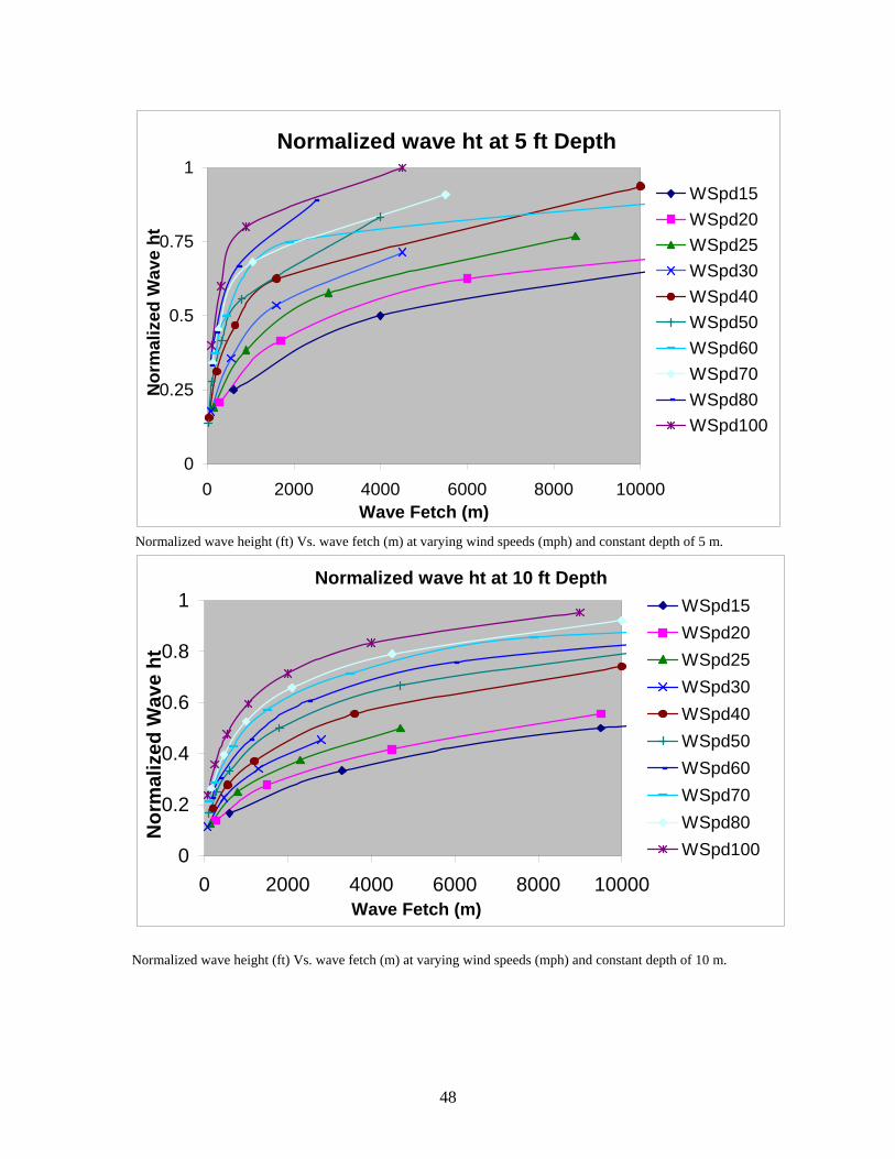
Graphs were normalized for wave height to project it on the same scale as the IDW power function graphs. The normalization is done using the maximum wave height attained by a wave for a particular wind speed and depth. For example, maximum height attained by a wave at 60 mph and a water depth of 5 ft is 2 ft, so all wave heights were normalized by 2 ft. The next two graphs show normalized wave height graphs for 5 ft and 10 ft water depths.

47

Normalized wave ht at 5 ft Depth

0

0.25

0.5

0.75

1

0 2000 4000 6000 8000 10000Wave Fetch (m)

Nor

mal

ized

Wav

e ht

WSpd15WSpd20WSpd25WSpd30WSpd40WSpd50WSpd60WSpd70WSpd80WSpd100

Normalized wave height (ft) Vs. wave fetch (m) at varying wind speeds (mph) and constant depth of 5 m.

Normalized wave ht at 10 ft Depth

0

0.2

0.4

0.6

0.8

1

0 2000 4000 6000 8000 10000Wave Fetch (m)

Nor

mal

ized

Wav

e ht

WSpd15WSpd20WSpd25WSpd30WSpd40WSpd50WSpd60WSpd70WSpd80WSpd100

Normalized wave height (ft) Vs. wave fetch (m) at varying wind speeds (mph) and constant depth of 10 m.

48

After normalization of the curves, a power function was assigned to each curve for each depth. The power functions for all the wind speeds are shown in the table below for each of the depths.

mph 10ft 5ft

15 y = 0.0154x0.3757 y = 0.0277x0.3448

20 y = 0.0156x0.3906 y = 0.036x0.3209

25 y = 0.0168x0.4016 y = 0.0348x0.3477

30 y = 0.0205x0.391 y = 0.0393x0.3488

40 y = 0.0283x0.359 y = 0.0516x0.327

50 y = 0.0347x0.3466 y = 0.0673x0.304

60 y = 0.0478x0.314 y = 0.1361x0.2084

70 y = 0.0643x0.2809 y = 0.1036x0.2586

80 y = 0.0597x0.3055 y = 0.0978x0.2865

100 y = 0.0689x0.2996 y = 0.1434x0.2391

Power function for wind speeds at 5 m and 10 m depths. To make the final wave generation function, wind speed was divided into 3 categories and each category was assigned a power function derived by averaging the powers from that category from the above table. Three categories are for 5 ft depth 0 – 30 mph 0.33 30+ – 60 mph 0.30 > 60+ mph 0.25 Three categories are for 10 ft depth 0 – 30 mph 0.39 30+ – 60 mph 0.35 > 60+ mph 0.29 To implement these results in the IDW function, a decay curve for the IDW function was plotted from the equation:

IDW = 1/(distance + 1) z (1 – distance / fetch)

49

Where distance is the cumulative distance from the site, fetch is the maximum wave fetch selected in WEMo options and z is the power to be derived. The decay curve was converted into a cumulative curve to emulate the SPM curves derived above. The power z was then derived for each of the wind category 0 – 30 mph 0.053 30+ – 60 mph 0.062 > 60+ mph 0.082 These are the recommended power functions for three assigned categories, used to calculate REI in WEMo. The graph below shows the cumulative IDW function for three categories. The next graph shows the IDW function for three wind speed categories.

Cumulative inverse distance weighting for three wind speed categories

0

0.2

0.4

0.6

0.8

1

0 2000 4000 6000 8000 10000Wave Fetch (mt)

IDW 0 - 30mph

31 - 60mph

> 60mph

Cumulative IDW function for three wind speed categories

50

Inverse distance weighting for three wind speed categories

0

0.2

0.4

0.6

0.8

1

0 2000 4000 6000 8000 10000Wave Fetch (mt)

IDW

IDW 0 - 30mph

IDW 31 - 60mph

IDW >60mph

IDW function for three wind speed categories

After assigning a power function for each wind category, each ray generated from the site in the 8 compass heading directions will have a power for use in the IDW function. However, the 4 rays radiating out from either side of the ith compass heading at increments of 11.25 degrees, will not have any associated wind speed, hence they do not have a power value to utilize in the IDW function. To assign a power for intermediate rays, a linearized average function was used between adjacent ith compass headings to calculate intermediate powers. For example, if easting has power of 0.082 and northing has power of 0.062 then, 1st intermediate rays power –> 0.082 + (0.062 – 0.082)/4 = 0.077 2nd intermediate rays power –> 0.082 + 2*(0.062 – 0.082)/4 = 0.072 3rd intermediate rays power –> 0.082 + 3*(0.062 – 0.082)/4 = 0.067 There is an option to change these power functions as well as wind categories in WEMo as explained elsewhere in the manual. However, increasing the number of categories increases the processing time while significantly decreasing a function causes coarse results. It is recommended that without specific cause for selecting other options that the user adopts the default values described above.

51

Appendix B This ArcView 3.2 avenue scripts convert an ungenerate format vector file downloaded from NGDC website into ArcView shapefile format. Please copy and paste it in the ArcView script window and compile it before running. Script obtained from NGDC website. Script Starts ' Generate2Shape ' Originally based on GPS2Shape by GAT, GEODATA AS ' Converts a file with ARC/INFO Generate format to a AV2 Shape file ' ' Ver. 1 by GAT, GEODATA AS Dec, 28 1994 ' ARC/INFO Generate format for lines implemented ' Format: ' ID ' x,y ' . ' . ' x,y ' END ' ID ' x,y ' . ' . ' x,y ' END ' END ' Choose the Generate file to convert to shapefile... genName = FileDialog.Show("*.*","Generate File","Select Generate File to Convert") if (genName = nil) then exit end genFile = LineFile.Make(genName, #FILE_PERM_READ) totalRecs = genFile.GetSize ' Specify the output shapefile... ' defaultName = FN.Make("$HOME").MakeTmp("shape","shp") shpName = FileDialog.Put( defaultName,"*.shp","Output Shape File" ) if (shpName = nil) then exit end

52

shpName.SetExtension("shp") ' Specify which kind of shapefile to create and make the new FTab... ' In current version (1.0) only line ' type = MsgBox.ChoiceAsString({"Line"}, "Convert coordinates to:", "Generate Convert" ) if (type = Nil) then exit end if (type = "Point") then shpFTab = Ftab.MakeNew(shpName,Point) elseif (type = "Line") then shpFTab = FTab.MakeNew(shpName, Polyline) elseif (type = "Polygon") then shpFTab = FTab.MakeNew(shpName, Polygon) end fields = List.Make fields.Add(Field.Make("ID", #FIELD_LONG, 4, 0)) shpFTab.AddFields(fields) shpField = shpFTab.FindField("Shape") idField = shpFTab.FindField("ID") genRec = 0 av.ShowStopButton av.ShowMsg("Converting"++genName.GetBaseName+"...") ' If the user has chosen 'Point' then the FTab is written here in the ' while loop. Otherwise if 'Line' or 'Polygon' has been chosen we ' collect coordinates in the loop for writing to the FTab later... while (true) buf = genFile.ReadElt if (buf = Nil) then break end if (buf = "END") then break end

53

if ((type = "Line") or (type = "Polygon")) then pointList = List.Make theID = buf buf = genFile.ReadElt end while (true) genTokens = buf.AsTokens(",") if (type = "Point") then ' write points to FTab... theID = genTokens.Get(0) thePoint = genTokens.Get(1).AsNumber@genTokens.Get(2).AsNumber rec = shpFTab.AddRecord shpFTab.SetValueNumber( idField, rec, theID.AsNumber ) shpFTab.SetValue( shpField, rec, thePoint ) elseif (type = "Line") then ' collect points defining line... thePoint = genTokens.Get(0).AsNumber@genTokens.Get(1).AsNumber pointList.Add( thePoint ) elseif (type = "Polygon") then ' collect points defining polygon... thePoint = genTokens.Get(1).AsNumber@genTokens.Get(2).AsNumber pointList.Add( thePoint ) end genRec = genRec + 1 progress = (genRec / totalRecs) * 100 proceed = av.SetStatus( progress ) if (proceed.Not) then av.ClearStatus av.ShowMsg( "Stopped" ) exit end buf = genFile.ReadElt if (buf = Nil) then break end if (buf = "END") then break end end ' If Line or Polygon we still need to create FTab...

54

' if (type = "Line") then rec = shpFTab.AddRecord shpFTab.SetValueNumber( idField, rec, theID.AsNumber) pl = Polyline.Make( {pointList} ) shpFTab.SetValue( shpField, rec, pl ) elseif (type = "Polygon") then rec = shpFTab.AddRecord shpFTab.SetValueNumber( idField, rec, 1 ) ' Add first point to end of list to close the polygon... startPoint = pointList.Get(0) pointList.Add( startPoint ) pl = Polygon.Make( {pointList} ) shpFTab.SetValue( shpField, rec, pl ) end end av.ClearStatus av.ClearMsg shpFTab.Flush MsgBox.Info( genRec.AsString++"records converted." ,"Conversion Completed" ) Scripts End

55

Appendix C Step-by-step guide on creating a point-grid of values using ArcGIS Sometimes exposure values are desired for a larger whole area of interest in a grid format as opposed to few selected sites. Output from such a process provides the data needed to generate a surface response (e.g., krigged) for a pleasing graphic (this is beyond the scope of this help document). Creation of a grid dataset can be accomplished by creating a point grid using ArcGIS tools. This appendix explains in a step-by-step fashion how to create the regular grid with desired resolution. ArcGIS model To simplify the steps in creating a grid, we created an ArcGIS model that can be loaded in the toolbox to automate all the steps except creating the polygon shapefile (see below). A more detailed description of the process is given after this section. This model is provided in the WEMo installation and should be available in folder ‘Help’ under WEMo installation folder. A schematic of the model is shown below:

To load the model in ArcGIS, right click inside the open area in ArcToolbox window and select ‘Add Toolbox’ navigate to the Help folder where ‘Point Grid.tbx’ toolbox is saved. This will add the Point Grid toolbox in the list of toolboxes in ArcToolbox window. Double click the ‘Point grid tool’ tool and this will open up the parameter window shown below.

56

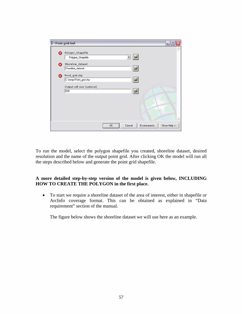
To run the model, select the polygon shapefile you created, shoreline dataset, desired resolution and the name of the output point grid. After clicking OK the model will run all the steps described below and generate the point grid shapefile. A more detailed step-by-step version of the model is given below, INCLUDING HOW TO CREATE THE POLYGON in the first place.

• To start we require a shoreline dataset of the area of interest, either in shapefile or ArcInfo coverage format. This can be obtained as explained in “Data requirement” section of the manual.

The figure below shows the shoreline dataset we will use here as an example.

57

CREATION OF THE EMPTY POLYGON SHAPEFILE NEEDED TO RUN THE MODEL, ABOVE

• After loading the shoreline file in ArcGIS create an empty polygon shapefile using ArcCatalog. Open ArcCatalog either from ArcMap window or from the Start ArcGIS ArcCatalog.

• In ArcCatalog window navigate to the desired folder and right click to select New Shapefile.

• In the Create New Shapefile window make sure to select ‘Feature Type’ as ‘Polygon’ and select the name of the shapefile shown in figure below.

58

59

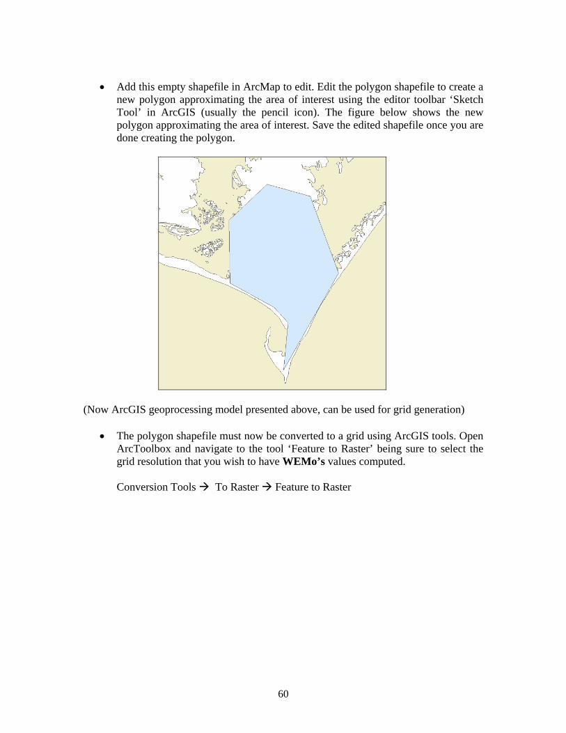
• Add this empty shapefile in ArcMap to edit. Edit the polygon shapefile to create a

new polygon approximating the area of interest using the editor toolbar ‘Sketch Tool’ in ArcGIS (usually the pencil icon). The figure below shows the new polygon approximating the area of interest. Save the edited shapefile once you are done creating the polygon.

(Now ArcGIS geoprocessing model presented above, can be used for grid generation)

• The polygon shapefile must now be converted to a grid using ArcGIS tools. Open ArcToolbox and navigate to the tool ‘Feature to Raster’ being sure to select the grid resolution that you wish to have WEMo’s values computed.

Conversion Tools To Raster Feature to Raster

60

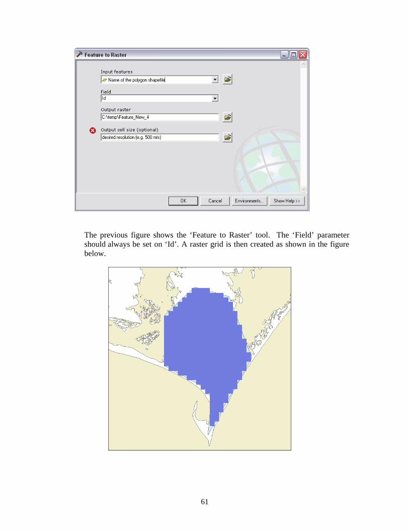
The previous figure shows the ‘Feature to Raster’ tool. The ‘Field’ parameter should always be set on ‘Id’. A raster grid is then created as shown in the figure below.

61

• In the next step this grid is converted into a point shapefile, where each point is created at the center of the grid cell. To create the point shapefile use the tool ‘Raster to Point’

Conversion Tools From Raster Raster to Point

• This tool creates the point dataset covering the area of polygon shapefile with the desired resolution. The example below shows the point grid at 500 meter resolution (as selected previously).

Note: Remember that every doubling of the resolution of the point grid increases the computational time four-fold. In most of the cases 500 meters is a desired resolution. Where bathymetry is uneven and shoreline is complex, higher resolution grids should be used though only for small areas.

62

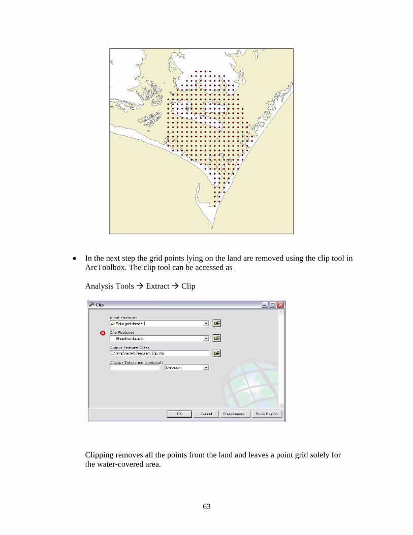
• In the next step the grid points lying on the land are removed using the clip tool in ArcToolbox. The clip tool can be accessed as

Analysis Tools Extract Clip

Clipping removes all the points from the land and leaves a point grid solely for the water-covered area.

63

The created point grid is an ArcGIS shapefile and is ready to be processed in WEMo successively. (Refer to ‘Adding point datasets’ section ‘Using external point dataset method’).

64

Contact Information Model Designed by: Mark S. Fonseca Ph.D. Leader, Applied Ecology and Restoration Research Branch NOAA, National Ocean Service National Centers for Coastal Ocean Science Center for Coastal Fisheries and Habitat Research 101 Pivers Island Rd Beaufort, NC 28516-9722 (252) 728 8729 office (252) 723 7102 cell (252) 728 8784 fax mark.fonseca@noaa.gov WEMo Software Designed by: Amit Malhotra GIS Analyst NOAA/NOS Beaufort Lab Beaufort, North Carolina 28516 (252) 728 8720 amit.Malhotra@noaa.gov

65

References consulted and suggested reading: Fonseca, M.S., B. D. Robbins, P.E. Whitfield, L. Wood and P. Clinton. 2002. Evaluating the effect of offshore sandbars on seagrass recovery and restoration in Tampa Bay through ecological forecasting and hindcasting of exposure to waves. Tampa Bay Estuary Program, St. Petersburg, Florida. Fonseca, M. S., J. C. Zieman, G.W. Thayer, and J. S. Fisher. 1983. The role of current velocity in structuring eelgrass (Zostera marina L.) meadows. Est. Coast. Shelf. Sci. 17:367-380. Fonseca, M.S. W.J. Kenworthy, F.X. Courtney, and M.O. Hall. 1994. Seagrass planting in the southeastern United States: methods for accelerating habitat development. Rest. Ecol. 2:198-212. Fonseca, M.S., S.S. Bell. 1998. Influence of physical setting on seagrass landscapes near Beaufort, North Carolina, USA. Mar. Ecol. Prog. Ser. 171:109-121. Fonseca M.S., W.J. Kenworthy and E. Paling 1998a. Restoring seagrass ecosystems in high disturbance environments. In Ocean Community Conference, Nov 16-19, 1998, Baltimore, MD. 6 p Fonseca, M.S., W.J. Kenworthy, G.W. Thayer. 1998b. Guidelines for the conservation and restoration of seagrass in the United States and adjacent waters. NOAA COP/Decision Analysis Series. #12, 222p Fonseca, M.S., W.J. Kenworthy, and P.E. Whitfield. 2000. Temporal dynamics of seagrass landscapes: a preliminary comparison of chronic and extreme disturbance events. p. 373-376. In Pergent, G., Pergent-Martini, C., Buia, M.C., and Gambi, M.C., (eds.), Proceedings 4th International Seagrass Biology Workshop, Sept. 25-Oct. 2, 2000, Corsica, France Fonseca, M.S., P.E. Whitfield, N.M. Kelly, S.S. Bell 2002. Modeling seagrass landscape pattern and associated ecological attributes. Ecol. Appl. 12:218-237 Johansson, J. 0. R, and R. R. Lewis. 1992. Recent improvements of water quality and biological indicators in Hillsborough Bay, a highly impacted subdivision of Tampa Bay, Florida, USA International Conference on Marine Coastal Eutrophication, Bologna, Italy, March 1990. Pp. 1199-1215 in Science of the Total Environment, Supplement 1992. Elsevier Publishers, Amsterdam. 1310 pp. Keddy, P.A. 1982. Quantifying within-lake gradients of wave energy: interrelationships of wave energy, substrate particle size and shoreline plants in Axe Lake, Ontario Aquatic Botany 14: 41-58.

66

Kelly, N.M., M. Fonseca, P. Whitfield. 2001. Predictive mapping for management and conservation of seagrass beds in North Carolina. Aq. Cons. Mar. and Freshwater Ecosys. 11:437-451. Lewis, R.R. 2002. The potential importance of the longshore bar system to the persistence and restoration of Tampa Bay seagrass meadows. Proceedings of the conference on “Seagrass Management: It’s Not Just Nutrients. August 22-24, 2000. St. Petersburg, Florida. Lewis, R. R., M. J. Durako, M.D. Moffler and R. C. Phillips. 1985. Seagrass meadows of Tampa Bay. Pp.210-246 in S. F. Treat, J. L. Simon, R. R. Lewis III and R. L Whitman, Jr. (eds.), Proceedings, Tampa Bay Area Scientific Information Symposium [May 1982]. Burgess Publishing Co., Minneapolis. 663 pp. Lewis, R. R., C. Kruer, S. Treat and S. Morris. 1994. Wetland Mitigation Evaluation Report, Florida Keys Bridge Replacement. Florida Dept. of Transportation WPI No.6116901, SP No. 90000-1560. 88 pp. + appends. Lewis, R. R., P. Clark, W. K. Fehring, H.S. Greening, R. Johansson and R. T. Paul. 1998. The rehabilitation of the Tampa Bay estuary, Florida, USA, an example of successful integrated coastal management. Marine Pollution Bulletin 37 (8-12): 468-473. Narumalani, S., J.R. Jensen, J.D. Althausen, J.D. Burkhalter, and S. Mackey. 1997. Aquatic macrophyte modeling using GIS and logistic multiple regression. Photogrammetric Engineering and Remote Sensing 63:41-49. Robbins, B.D. and S.S. Bell. 1994. Seagrass landscapes: a terrestrial approach to the marine subtidal environment. Trends in Ecology and Evolution. 9:301-304. Robbins, B.D. and S.S. Bell. 2000. Dynamics of a subtidal seagrass landscape: seasonal and annual change in relation to water depth. Ecol. 81:1193-1205. Robbins, B.D., M.S. Fonseca, P.W. Whitfield and P. Clinton. 2002. Use of a wave exposure technique for predicting distribution and ecological characteristics of seagrass ecosystems. P171-176 in Greening, H.S., editor. 2002. Seagrass Management: It’s Not Just Nutrients! 2000 Aug 22–24; St. Petersburg, FL. Tampa Bay Estuary Program. 246 p. Exploring ArcObjectsTM Vol 1 – Applications and Cartography. ESRI publications, Redlands, CA Exploring ArcObjectsTM Vol 1I – Geographic Data Management. ESRI publications, Redlands, CA Shore Protection Manual. 1977. US Army Coastal Engineering Research Center Ft Belvoir, VA.

67

68

Suchanek, T. H. 1983. Control of seagrass communities and sediment distribution by Callianassa (Crustacea; Thalassinidea) bioturbation. J. Mar. Res. 41:281-298.