Wellbore Strengthening by Means of Nanoparticle-Based ...

University of Calgary

PRISM: University of Calgary's Digital Repository

Graduate Studies The Vault: Electronic Theses and Dissertations

2014-04-02

Wellbore Strengthening by Means of

Nanoparticle-Based Drilling Fluids

Contreras Puerto, Oscar

Contreras Puerto, O. (2014). Wellbore Strengthening by Means of Nanoparticle-Based Drilling

Fluids (Unpublished doctoral thesis). University of Calgary, Calgary, AB.

doi:10.11575/PRISM/28684

http://hdl.handle.net/11023/1398

doctoral thesis

University of Calgary graduate students retain copyright ownership and moral rights for their

thesis. You may use this material in any way that is permitted by the Copyright Act or through

licensing that has been assigned to the document. For uses that are not allowable under

copyright legislation or licensing, you are required to seek permission.

Downloaded from PRISM: https://prism.ucalgary.ca

UNIVERSITY OF CALGARY

Wellbore Strengthening by Means of Nanoparticle-Based Drilling Fluids

by

Oscar Michel Contreras Puerto

A THESIS

SUBMITTED TO THE FACULTY OF GRADUATE STUDIES

IN PARTIAL FULFILMENT OF THE REQUIREMENTS FOR THE

DEGREE OF DOCTOR OF PHILOSOPHY

DEPARTMENT OF CHEMICAL AND PETROLEUM ENGINEERING

CALGARY, ALBERTA

April, 2014

© Oscar Michel Contreras Puerto 2014

ii

Abstract

Wellbore strengthening is the mechanism of increasing the fracture pressure of the rock at depth.

Application of wellbore strengthening in the drilling industry enable safe drilling by preventing

mud losses, drilling in narrow mud windows, accessing reserves in depleted reservoirs, and also

has the potential to reduce the number of casing runs. Until now, the predominant wellbore

strengthening mechanism and its occurrence in ultra-low permeability media such as shales is a

subject of discussion. This dissertation presents original research that concludes that fracture tip

resistance by the development of an immobile mass is the predominant wellbore strengthening

mechanism for sandstone and shale formations. Wellbore strengthening in sandstones and shales

was achieved with a fracture breakdown pressure increase of 65% and 30%, respectively. Oil

based mud (OBM) containing in-house prepared nanoparticles (NPs) was used for hydraulic

fracturing experiments performed in an experimental set-up that scaled a drilled, cased and

cemented wellbore in a core. Optical microscopy, scanning electron microscope (SEM), and

energy-dispersive X-ray spectroscopy (EDX) analysis were performed on the cores post-testing

and the fracture seal was characterized. This research demonstrated the successful application of

nanoparticle-based drilling fluids in the presence of graphite in reducing mud filtration at high-

pressure high-temperature (HPHT) in porous media and low-pressure low-temperature (LPLT) in

filter paper. Mud filtration reductions of 76% and 100% were achieved respectively. A strong

match between wellbore strengthening and mud filtration was discovered for iron-based (NP1)

and calcium-based (NP2) NPs. NPs performance in virgin vs. recycled mud was quantified and

the effect of NPs preparation procedure on blends performance was addressed. These results are

anticipated to have a significant impact in drilling and completions operations. This dissertation

iii

was conducted by the author in a cooperative agreement between the University of Calgary and

the Missouri University of Science and Technology.

iv

Acknowledgements

I would like to express my feelings of gratitude to my advisors Dr. Geir Hareland and Dr. Maen

Husein for their teaching, guidance and encouragement during my doctoral studies at the

University of Calgary. I acknowledge NSERC, Talisman Energy and Pason Systems for

providing the funding to this research work.

I wish to thank Dr. Runar Nygaard, my advisor at the Missouri University of Science and

Technology. His valuable technical support and words of motivation played a crucial role in the

development of this work. I would like to thank Dr. Azra Tutuncu from Colorado School of

Mines for her technical advices and useful comments that helped in the experimental stage.

Special thanks to Mr. Mortadha Alsaba and Mr. Michael Bassett from the Missouri University of

Science and Technology for their strong support in the conduction of the experiments and advice

in the development of the samples preparation protocols. I want to extend my feelings of

gratitude to my friends Carlos Castano, Carlos Sanchez, and Angelica Alvarez for their support

in my stay in Rolla, Missouri.

Finally I would like to acknowledge Mr. Nisael Solano and Mr. Chris DeBuhr from the

Geoscience Department at the University of Calgary for their technical assistance on the samples

post-testing analysis.

v

Dedication

To my parents Oscar Alberto y Carmen Elisa

To by brother Satchel Fabricio

To my grandmother Ubaldina

To my girlfriend Enna Rocio

vi

Table of Contents

Abstract ............................................................................................................................... ii Acknowledgements ............................................................................................................ iv

Dedication ............................................................................................................................v Table of Contents ............................................................................................................... vi List of Tables ..................................................................................................................... ix List of Figures and Illustrations ...........................................................................................x List of Symbols, Abbreviations and Nomenclature ......................................................... xix

INTRODUCTION ..................................................................................1 CHAPTER ONE:

1.1 Justification ................................................................................................................1 1.2 Research Objectives ...................................................................................................2

1.3 Oil Based Mud Applications ......................................................................................3 1.4 Common Drilling Challenges ....................................................................................6

1.4.1 Lost circulation ..................................................................................................6

1.4.2 Stuck pipe ..........................................................................................................9 1.4.3 Wellbore instability .........................................................................................11

1.5 Nanoparticles Applications in Drilling Industry ......................................................14 1.6 Dissertation Chapters Description ...........................................................................18 1.7 Technical Publications .............................................................................................20

WELLBORE STRENGTHENING .....................................................22 CHAPTER TWO:

2.1 Introduction to Wellbore Strengthening ..................................................................22

2.2 Motivation: Potential Impact of Wellbore Strengthening in Western Canada ........25

2.2.1 Technical analysis ...........................................................................................26

2.2.2 Economic impact .............................................................................................29 2.3 Literature Review on Wellbore Strengthening Methods .........................................32

2.3.1 DEA-13 project ...............................................................................................32 2.3.2 GPRI Joint Industry Project (JIP) ....................................................................34 2.3.3 Stress caging theory .........................................................................................34

2.3.4 Tip Resistance by development of an immobile mass ....................................37 2.3.5 Sealing of wellbore by filter cake ....................................................................38

2.3.6 Fracture propagation resistance (FPR) ............................................................39 2.3.7 Numerical simulation of fracture propagation and sealing .............................41

2.3.8 Experimental analysis and mechanistic modeling of wellbore strengthening .42 2.3.9 Wellbore strengthening-nano-particle drilling fluid experimental design using a

hydraulic fracture apparatus .............................................................................43 2.3.10 Other wellbore strengthening mechanisms ...................................................45 2.3.11 Discussion of wellbore strengthening mechanisms .......................................46

NANOPARTICLES APPLICATION FOR MUD FILTRATION CHAPTER THREE:

CONTROL ................................................................................................................48

3.1 Introduction to NPs Application for Mud Filtration Control ...................................48 3.2 Experimental Methods .............................................................................................49

3.2.1 Drilling fluid characterization .........................................................................49

3.2.2 NPs characterization ........................................................................................50

vii

3.2.3 LCM Characterization .....................................................................................50

3.3 Establishment of Concentration Limits ...................................................................52 3.4 Introduction to the Experimental Analyses .............................................................53 3.5 Filtration Devices .....................................................................................................54

3.6 Drilling Fluid Mixing ...............................................................................................55 3.7 Nanoparticle Preparation Procedure ........................................................................55

3.7.1 NP1 mixing procedure .....................................................................................56 3.7.2 NP2 mixing procedure .....................................................................................57 3.7.3 Rheology analysis ............................................................................................58

3.8 LPLT Filtration Analysis .........................................................................................60 3.9 HPHT Filtration Analysis ........................................................................................65 3.10 Summary ................................................................................................................73

NANOPARTICLES APPLICATION FOR WELLBORE CHAPTER FOUR:

STRENGTHENING IN SANDSTONE CORES .....................................................75 4.1 Introduction to the Experimental Analysis ..............................................................75

4.2 Experimental Facilities and Apparatus ....................................................................76 4.3 Sandstone Cores Characterization ...........................................................................84

4.3.1 Composition ....................................................................................................84 4.3.2 Porosity and permeability ................................................................................84 4.3.3 Tensile strength ...............................................................................................85

4.4 Sandstone Cores Preparation ...................................................................................86 4.4.1 Drilling of 5

3/4” cores from slabs .....................................................................87

4.4.2 Drilling of 9/16” wellbore in the center of the cores .......................................88 4.4.3 Casing assembly on steel caps and caps cementing on cores ..........................89

4.4.4 Cement dry out ................................................................................................91 4.4.5 Core surface grinder ........................................................................................91

4.4.6 Core vacuuming and saturation .......................................................................92 4.4.7 Post-testing caps cleaning ................................................................................93

4.5 Challenges Faced and Solutions in Sandstone Cores Preparation ...........................93

4.5.1 Drilling a straight wellbore in the center of the cores .....................................94 4.5.2 Removal of a natural fracture from cores ........................................................95

4.6 Wellbore Strengthening Tests using a Hydraulic Fracturing Apparatus .................96 4.6.1 Experimental procedure for testing of sandstone cores ...................................96

4.6.2 Wellbore strengthening results ........................................................................97 4.6.3 Challenges encountered during wellbore strengthening tests .......................114

4.7 Sandstone Cores Post-testing Analysis ..................................................................115

4.8 Results Analysis and Identification of Predominant Wellbore Strengthening

Mechanism ...........................................................................................................118 4.8.1 Results analysis of wellbore strengthening in sandstone cores .....................118 4.8.2 Identification of predominant wellbore strengthening mechanism ...............121

4.9 Summary ................................................................................................................128

NANOPARTICLES APPLICATION FOR WELLBORE CHAPTER FIVE:

STRENGTHENING IN SHALE CORES ..............................................................131 5.1 Introduction to the Experimental Analysis ............................................................131 5.2 Experimental Facilities and Apparatus ..................................................................132

viii

5.3 Shale Cores Characterization .................................................................................133

5.3.1 Composition ..................................................................................................133 5.3.2 Porosity and permeability ..............................................................................133 5.3.3 Tensile strength .............................................................................................135

5.4 Shale Cores Preparation .........................................................................................137 5.4.1 Drilling of 9/16” wellbore in the center of the cores .....................................138 5.4.2 Casing assembly on steel caps and cementing of caps in cores ....................139 5.4.3 Cement dry out ..............................................................................................140

5.5 Challenges Faced and Solutions in Shale Cores Preparation ................................141

5.5.1 Drilling of wellbore in the center ..................................................................142 5.5.2 Steel caps cementing .....................................................................................143

5.6 Wellbore Strengthening Tests using a Hydraulic Fracturing Apparatus ...............143 5.6.1 Experimental procedure for testing of shale cores ........................................143

5.6.2 Wellbore strengthening results ......................................................................144 5.6.3 Challenges faced in wellbore strengthening tests ..........................................157

5.7 Shale Cores Post-testing Analysis .........................................................................165 5.8 Results Analysis and Proposed Mechanism for Wellbore Strengthening in Shale Cores

..............................................................................................................................168 5.8.1 Results analysis of wellbore strengthening in shale cores .............................168 5.8.2 Proposed mechanism for wellbore strengthening in shale cores ...................171

5.9 Summary ................................................................................................................178

CONCLUSIONS, ORIGINAL CONTRIBUTIONS TO KNOWLEDGE CHAPTER SIX:

AND RECOMMENDATIONS ..............................................................................181 6.1 General Remarks ....................................................................................................181

6.2 Conclusions ............................................................................................................181 6.3 Original Contributions to Knowledge ....................................................................183

6.4 Recommendations ..................................................................................................184

REFERENCES ................................................................................................................186

ix

List of Tables

Table 1-1: Advantages and disadvantages of OBM (Bourgoyne et al., 1986). .............................. 5

Table 2-1: Drilling costs for well A from AFE. ............................................................................ 30

Table 2-2: Drilling costs for well B from AFE. ............................................................................ 31

Table 2-3: Differences on techniques for wellbore strengthening. ............................................... 39

Table 3-1: OBM composition and rheology. ................................................................................ 49

Table 3-2: Graphite chemical properties (courtesy of Bri-Chem). ............................................... 51

Table 3-3: Graphite particle size distribution (courtesy of Bri-Chem). ........................................ 51

Table 3-4: Tests matrices for rheology testing of NP1 and NP2. ................................................. 58

Table 3-5: Rheology results for all blends (DF stands for iron-based blends and DC1 stands

for calcium-based blends). .................................................................................................... 59

Table 4-1: Sandstone porosity results. .......................................................................................... 85

Table 4-2: Sandstone permeability results. ................................................................................... 85

Table 4-3: Tensile strength for the three sandstone slabs. ............................................................ 86

Table 4-4: Hydraulic fracturing experiment checklist. ................................................................. 98

Table 4-5: Hydraulic fracturing experiment check list – Post testing. ......................................... 99

Table 4-6: Steps for refilling while running a test and pumping after refilling. ........................... 99

Table 4-7: Tests matrices for wellbore strengthening in sandstone cores. ................................. 100

Table 5-1: Catoosa shale composition (Andersen and Azar, 1993). ........................................... 133

x

List of Figures and Illustrations

Figure 1.1: Most common drilling problems. ................................................................................. 1

Figure 1.2: Schematic of a stable emulsion (M-I Swaco drilling fluid manual)............................. 4

Figure 1.3: Sensitive formations for mud losses (Alsaba et al., 2014). .......................................... 7

Figure 1.4: Mechanical stuck pipe (modified from M-I Swaco drilling fluid manual). ............... 10

Figure 1.5: Cuttings settlement and stuck pipe (M-I Swaco drilling fluid manual). .................... 10

Figure 1.6: Mechanics of differential sticking (M-I Swaco drilling fluid manual). ..................... 11

Figure 1.7: Results of wellbore instabilities (M-I Swaco drilling fluid manual). ......................... 13

Figure 1.8: Wellbore breakout (modified from Zoback, 2007). ................................................... 13

Figure 1.9: Schematic of a XLOT (Tutuncu, 2010)...................................................................... 15

Figure 1.10: Effect of NPs in reducing mud filtration towards the formation. ............................. 16

Figure 1.11: Area to volume ratio of three different sizes of particles (Amanullah and Al-

Tahini, 2009). ........................................................................................................................ 17

Figure 1.12: Arrangement of nanosilica particles of 20 nm mean diameter viewed under the

TEM (Riley et al., 2012). ...................................................................................................... 17

Figure 2.1: Mud window narrowing by different conditions (Alsaba et al., 2013). ..................... 23

Figure 2.2: In-situ stresses acting in a determined volume of earth crust (Tutuncu, 2010).......... 23

Figure 2.3: Deep Basin of the WCSB (modified from Masters, 1984). ....................................... 26

Figure 2.4: (a) Mud window for well A and definition of casing setting depths. Red profiles

correspond to average values of pore pressure gradient and fracture gradient. (b) Mud

window for well A and definition of casing setting depths after wellbore strengthening.

Red profiles correspond to average values of pore pressure gradient and fracture

gradient. ................................................................................................................................ 28

Figure 2.5: (a) Mud window for well B and definition of casing setting depths. Red profiles


window for well B and definition of casing setting depths after wellbore strengthening.

Red profiles correspond to average values of pore pressure gradient and fracture

gradient. ................................................................................................................................ 28

Figure 2.6: Similar initial fracture breakdown pressure using water and oil-based muds

(Morita et al., 1996). ............................................................................................................. 33

xi

Figure 2.7: Core after hydraulic fracturing experiment (Wang, 2007). ........................................ 34

Figure 2.8: Stress caging theory. ................................................................................................... 35

Figure 2.9: Tip resistance by the development of an immobile mass. .......................................... 37

Figure 2.10: Test apparatus for WSMs screening and selection (Van oort et al., 2011). ............. 40

Figure 2.11: Hoop stress at wellbore after fracture sealing (black line), fracture propagation

(redline), fracture initiation (green line) and for intact wellbore (blue line) from Salehi

(2011). ................................................................................................................................... 41

Figure 2.12: Wellbore condition in LOT interpretation (Salehi, 2011). ....................................... 42

Figure 2.13: Core fracturing system set-up (Mostafavi, 2011). .................................................... 43

Figure 2.14: P vs. t plot for OBM containing NPs tested on sandstone core (Nwaoji, 2012). ..... 44

Figure 2.15: Elastic-plastic borehole fracture model (Aadnoy and Belayneh, 2004). .................. 45

Figure 2.16: Contrast between tip resistance by the development of an immobile mass and

stress caging mechanisms. .................................................................................................... 47

Figure 3.1: Glide graphite. ............................................................................................................ 51

Figure 3.2: Graphite precipitation after mixing. ........................................................................... 52

Figure 3.3: NP2 precursors precipitation after mixing. ................................................................ 53

Figure 3.4: 170-00-7 Ofite HPHT filter press. .............................................................................. 54

Figure 3.5: Paint mixer used to mix OBM. ................................................................................... 55

Figure 3.6: OBM mixing with hand drill. ..................................................................................... 55

Figure 3.7: Hamilton Beach 10-speed blender containing drilling fluid. ..................................... 56

Figure 3.8: (a) Percentage of reduction in mud filtration at 30 min under LPLT for NP1. (b)

Percentage of reduction in mud filtration at 30 min under LPLT for NP2. .......................... 61

Figure 3.9: Filter cake characterization for control sample and blends containing graphite at

low and high concentrations at LPLT. .................................................................................. 62

Figure 3.10: (a) Filter cake characterization for control blends containing NP1 at LPLT. (b)

Filter cake characterization for control blends containing NP2 at LPLT. ............................ 63

Figure 3.11: % filtrate reduction (left axis) compared to % filter cake thickness increase

(right axis) for (a) NP1 and (b) NP2. .................................................................................... 64

xii

Figure 3.12: (a) Percentage of reduction in mud filtration at 30 min under HPHT for NP1. (b)

Percentage of reduction in mud filtration at 30 min under HPHT for NP2. 775 md

ceramic discs were used in the filtration experiments. ......................................................... 66

Figure 3.13: Filter cake characterization for CS and blends containing graphite at low and

high concentrations and blends containing just NP1 and NP2 respectively at HPHT. ......... 66

Figure 3.14: (a) Filter cake characterization for control blends containing NP1 at HPHT. (b)

Filter cake characterization for control blends containing NP2 at HPHT. ........................... 67

Figure 3.15: % HPHT filtrate reduction (left axis) compared to % filter cake thickness

increase (right axis) for (a) NP1 and (b) NP2. ...................................................................... 68

Figure 3.16: Percentage of reduction in mud filtration at 30min under HPHT for NP1. The

green dot represents the blend only containing NP1 at 0.5 wt%. ......................................... 70

Figure 3.17: Percentage of reduction in mud filtration at 30 min under HPHT for NP2. The

green dot represents the blend only containing NP2 at 2.5 wt%. ......................................... 71

Figure 3.18: Cross-section of ceramic disc after DF3 blend testing at HPHT. ............................ 71

Figure 3.19: SEM image of filter cake for blend (a) without NP1 and (b) with NP1 (Zakaria,

2013). .................................................................................................................................... 72

Figure 3.20: SEM image of filter cake for blend (a) without NP2 and (b) with NP2 (modified

from Zakaria, 2013). ............................................................................................................. 73

Figure 4.1: Rock drill. ................................................................................................................... 77

Figure 4.2: (a) Rock Saw. (b) Small samples saw. ....................................................................... 77

Figure 4.3: Grinder........................................................................................................................ 78

Figure 4.4: (a) D28710 14” chop saw. (b) Small angle grinders. ................................................. 78

Figure 4.5: Brazilian test apparatus. ............................................................................................. 79

Figure 4.6: Hydrualic fracturing apparatus. .................................................................................. 80

Figure 4.7: Schematic of hydraulic fracturing apparatus (Liberman, 2012)................................. 81

Figure 4.8: Isco DX100 syringe type pumps (Liberman, 2012). .................................................. 82

Figure 4.9: Mud accumulator system (Liberman, 2012). ............................................................. 82

Figure 4.10: Overburden piston (Liberman, 2012). ...................................................................... 83

Figure 4.11: Rubber sleeve top view. ........................................................................................... 83

xiii

Figure 4.12: Roubidoux sandstone slabs. ..................................................................................... 84

Figure 4.13: 2”x 1” Sandstone cores for porosity and permeability measurements. .................... 84

Figure 4.14: Sandstone cores after Brazilian test for (a) Slab 1, (b) Slab 2, and (c) Slab 3. ........ 86

Figure 4.15: (a) Sandstone core drilling arrangement. (b) Sandstone core drilling while

pumping water. ..................................................................................................................... 87

Figure 4.16: (a) Rock slab after drilling the first core. (b) Sandstone cores. ................................ 88

Figure 4.17: Wellbore drilling on sandstone core. ........................................................................ 88

Figure 4.18: (a) Wellbore drilling on sandstone core using a PVC guide. (b) Sandstone core

after wellbore drilling. .......................................................................................................... 89

Figure 4.19: Steel caps for top and bottom ends of cores. ............................................................ 90

Figure 4.20: (a) Epoxy. (b) Epoxy after mixing. .......................................................................... 90

Figure 4.21: Sandstone cores and steel caps cementing dry out using clamps. ............................ 91

Figure 4.22: Hand grinder for core surface. .................................................................................. 92

Figure 4.23: Sandstone core vacuuming arrangement. ................................................................. 92

Figure 4.24: Steel caps removing.................................................................................................. 93

Figure 4.25: Steel caps cleaning. .................................................................................................. 94

Figure 4.26: Wellbore cemented. .................................................................................................. 94

Figure 4.27: Natural fractures on sandstone rock slabs. ............................................................... 95

Figure 4.28: (a) Welding of steel support for core sliding. (b) Sandstone core on

steel support. ......................................................................................................................... 96

Figure 4.29: P vs. t plot for control sample................................................................................. 101

Figure 4.30: Core after control sample testing............................................................................ 101

Figure 4.31: P vs. t plot for DC1 indicating the pressure increase. ............................................ 102

Figure 4.32: Core after DC1 testing. ........................................................................................... 103



xiv



Figure 4.37: P vs. t plot for DC6 indicating the significant pressure increase. .......................... 106

Figure 4.38: Core after DC6 testing. Note that vertical fractures are not visualized. ................. 107

Figure 4.39: Broken O-ring......................................................................................................... 107



Figure 4.42: P vs. t plot for DF1 indicating the pressure increase. ............................................. 109

Figure 4.43: Core after DF1 testing. ........................................................................................... 110







Figure 4.50: P vs. t plot for blend containing 0.5 wt% and 2.0 wt% of graphite........................ 113

Figure 4.51: Core after (a) 0.5 wt% and (b) 2.0 wt% of graphite blend testing. ........................ 114

Figure 4.52: Hydraulic jack working on pressure cell. ............................................................... 115

Figure 4.53: (a) Sandstone core after caps removing. (b) Top view of a sandstone core. Note

mud filtrate along hydraulic fracture plane. ........................................................................ 116

Figure 4.54: (a) Sandstone core used to obtain a disc for microscope analysis. (b) Microscope

analysis on sandstone core disc. .......................................................................................... 116

Figure 4.55: (a) Fracture at wellbore. (b) 3D representation of wellbore and vertical fracture. . 117

Figure 4.56: (a) Fracture at core end. (b) 3D representation of fracture at the core end. ........... 117

Figure 4.57: % Pfb increase vs. NP2 concentration in sandstone cores. ..................................... 118

Figure 4.58: % Pfb increase vs. NP1 concentration in sandstone cores. ..................................... 119

xv

Figure 4.59: % Pfb increase (left axis) compared to % HPHT filtrate reduction (right axis) for

NP2 blends at two graphite levels (a) 0.5 wt% (b) 2.0 wt%. .............................................. 120

Figure 4.60: % Pfb increase (left axis) compared to % HPHT filtrate reduction (right axis) for

NP1 blends at two graphite levels (a) 0.5 wt% (b) 2.0 wt%. .............................................. 121

Figure 4.61: Top view of a sandstone core disc.......................................................................... 122

Figure 4.62: Cross-section of sandstone disc along fracture plane. Note the presence of

graphite along the fracture plane. ........................................................................................ 123

Figure 4.63: (a) Top view of a sandstone core indicating the vertical fractures. (b) Top view

showing the same fracture with along the fracture. ............................................................ 123

Figure 4.64: Location and nomenclature of sandstone samples analyzed. ................................. 124

Figure 4.65: (a) Sandstone samples for SEM and EDX analysis. (b) Scanning electron

microscope. ......................................................................................................................... 124

Figure 4.66: SEM and EDX of fracture seal along a fracture plane cross-section indicating

the presence of calcium particles. ....................................................................................... 125

Figure 4.67: (a) NP2 at seal cross-section. (b) NP2 at fracture plane. Particles highlighted

with red arrows have size ≤150nm. .................................................................................... 126

Figure 4.68: EDX of Ca, Na, and Cl. Light blue color represents NaCl as a result of green

(Na) and blue (Cl) colors mixing. ....................................................................................... 127

Figure 4.69: Wellbore filter cake cross-section (left) and front view (right). ............................. 128

Figure 5.1: Drill press at RMERC. ............................................................................................. 132

Figure 5.2: Porosity vs. effective stress for Catoosa shale (Reyes and Osisanya, 2000)............ 134

Figure 5.3: Permeability vs. effective stress for Catoosa shale (Reyes and Osisanya, 2000). ... 134

Figure 5.4: (a) Core bit, drill press and shale core. (b) Set-up during drilling of 2”x1” cores.

(c) 2”x1” shale core............................................................................................................. 135

Figure 5.5: 2”x1” shale cores into mineral oil. On top: cores drilled parallel to wellbore. On

bottom: cores drilled perpendicular to wellbore containing black lines done with a

marker. ................................................................................................................................ 136

Figure 5.6: Shale samples drilled parallel to wellbore after Brazilian test (a) Replicate 1. (b)

Replicate 2. ......................................................................................................................... 136

Figure 5.7: Shale samples drilled perpendicular to wellbore after Brazilian test (a) Replicate

1. (b) Replicate 2. ................................................................................................................ 137

xvi

Figure 5.8: Compressive strength of Catoosa shale at various confining pressures (Andersen

and Azar, 1993). .................................................................................................................. 137

Figure 5.9: (a) Wrapped shale core. (b) Shale cores into mineral oil. (c) Shale core with a

mineral oil film exposed to air. ........................................................................................... 138

Figure 5.10: Shale core on drill press table for wellbore drilling. A 9/16” steel twist drill bit

was used for drilling. ........................................................................................................... 139

Figure 5.11: (a) Set-up for wellbore drilling. (b) Wellbore drilling. Note the drill cuttings

from drilling on the wood guide. ........................................................................................ 140

Figure 5.12: Cementing of shale cores. Note that the core is wrapped to avoid contact with

air. A contrast with a sandstone core cementing is illustrated. ........................................... 140

Figure 5.13: Shale core wrapped after cementing and prior to hydraulic fracturing test. .......... 141

Figure 5.14: Wood bit broken in two pieces. .............................................................................. 143

Figure 5.15: P vs. t plot for control sample in shale. .................................................................. 145

Figure 5.16: Core after control sample in shale testing. ............................................................. 145

Figure 5.17: P vs. t plot for DC4 Shale indicating the pressure increase. .................................. 146

Figure 5.18: Core after DC4 Shale testing. ................................................................................. 147

Figure 5.19: P vs. t plot for DC6 Shale indicating the pressure increase. .................................. 147

Figure 5.20: Core after DC6 Shale testing. ................................................................................. 148

Figure 5.21: P vs. t plot for DF1 Shale indicating the pressure increase. ................................... 148

Figure 5.22: Core after DF1 Shale testing. ................................................................................. 149

Figure 5.23: P vs. t plot for DF3 Shale indicating the pressure increase. ................................... 150

Figure 5.24: Core after DF3 Shale testing. ................................................................................. 150

Figure 5.25: Mixing of recycled mud for testing. ....................................................................... 151

Figure 5.26: P vs. t plot for Blackstone control sample in shale. ............................................... 151

Figure 5.27: Core after Blackstone control sample testing. ........................................................ 152

Figure 5.28: P vs. t plot for BDF-B3-I-05A indicating the pressure increase. ........................... 152

Figure 5.29: Core after BDF-B3-I-05A testing........................................................................... 153

xvii

Figure 5.30: P vs. t plot for BDF-B3-I-05C indicating the pressure increase. ........................... 154

Figure 5.31: Core after BDF-B3-I-05C testing. .......................................................................... 154

Figure 5.32: P vs. t plot for BDF-B3-C-3S indicating the pressure increase.............................. 155

Figure 5.33: Core after BDF-B3-C-3S testing. ........................................................................... 155

Figure 5.34: P vs. t plot for Blackstone blend containing 0.5 wt% of graphite. ......................... 156

Figure 5.35: Core after 0.5 wt% of graphite testing. .................................................................. 156

Figure 5.36: (a) Shale core from top cap after failure. (b) Shale core from top and bottom cap

after failure. (c) Shale segments inside pressure cell. ......................................................... 158

Figure 5.37: Rubber sleeve after shale core segments extraction. Red arrow indicates the

leakage area. ........................................................................................................................ 158

Figure 5.38: (a) Rubber sleeve. (b) Steel cylinder removal from bottom flange. (c) Placement

of a new rubber sleeve and silicon. ..................................................................................... 160

Figure 5.39: (a) Tape support for bottom cap. (b) Top view of pressure cell after core failure.

(c) Shale core after failure. .................................................................................................. 161

Figure 5.40: (a) Top view of pressure cell after core failure. (b) Shale core after failure. ......... 162

Figure 5.41: (a) Top view of pressure cell before testing. (b) Water leakage from rubber

sleeve on top pressure cell. ................................................................................................. 163

Figure 5.42: (a) Top and bottom gaskets. (b) SBR rubber strip for gasket manufacturing. ....... 164

Figure 5.43: New gasket on bottom flange. ................................................................................ 164

Figure 5.44: Shale core after testing. A vertical fracture can be observed. ................................ 165

Figure 5.45: (a) Core showing two vertical fractures. (b) Hirox Optical Digital microscope on

shale sample. ....................................................................................................................... 166

Figure 5.46: Top view of shale sample analyzed in Optical microscope. .................................. 166

Figure 5.47: (a) Shale core wellbore indicating two vertical fractures. (b) 3D illustration of

shale core wellbore.............................................................................................................. 167

Figure 5.48: (a) Shale core end indicating two vertical fractures. (b) 3D illustration of shale

core end. .............................................................................................................................. 167

Figure 5.49: % Pfb vs. NP2 concentration in shale cores. ........................................................... 168

Figure 5.50: %Pfb increase vs. NP1 concentration in shale cores. .............................................. 169

xviii

Figure 5.51: %Pfb increase compared to % HPHT filtrate reduction for NP2. ........................... 170

Figure 5.52: % Pfb increase vs. % HPHT filtrate reduction for NP2. Arrow indicates the

direction of NP1 concentration increase. ............................................................................ 171

Figure 5.53: Permeability vs. Porosity cross-plot including shale formations from Canada and

United States. Nikanassin tight gas formation data is also included and represented on

the top of the plot (Aguilera, 2013). The Blue square stands for the Catoosa shale at

testing conditions. ............................................................................................................... 173

Figure 5.54: Shale core cross-section along the fracture plane. ................................................. 173

Figure 5.55: Location and nomenclature of shale samples analyzed.......................................... 174

Figure 5.56: Shale samples for SEM and EDX analysis. ........................................................... 175

Figure 5.57: (a) Cross-section of fracture plane (2000x mag) close to wellbore. (b) Zoom in

seal (5000x mag) at fracture mouth. ................................................................................... 175

Figure 5.58: Zoom in seal at nano-scale (120000x mag). ........................................................... 176

Figure 5.59: (a) Cross-section of fracture plane (150x mag) far from wellbore. (b) Zoom in

seal (10000x mag) at fracture end. ...................................................................................... 177

Figure 5.60: Bulk of shale (2500x mag) only showing some pyrite agglomerations. ................ 177

Figure 5.61: Fracture plane image far from wellbore at (a) 600x mag and (b) 2400x mag.

Note graphite presence far from wellbore........................................................................... 178

Figure 5.62: (a) Seal cross-section (500x mag). (b) EDX of seal cross-section (500x mag).

Green color indicate iron particles distribution on seal. ..................................................... 178

xix

List of Symbols, Abbreviations and Nomenclature

Symbol Definition

b Eaton’s exponent, dimensionless

g Gravity, m/s2

K Permeability, md

Kb Kelly bushing elevation, m

P Pressure, psi

Pfi Pressure of the fluid into the fracture at time i, kPa

Pfb

Fracture breakdown pressure, psi

Pfb-deviated

Fracture breakdown pressure-deviated wells, psi

Pn* Modified water normal pressure, kPa

Pp Pore pressure, kPa

P*w Collapse pressure, kPa

Pwi Pressure in the wellbore at time i, kPa

rp35 Pore throat aperture, microns

R2 Coefficient of determination, dimensionless

t Time, s or min (as indicated)

T Temperature, °C or °F (as indicated)

To

Tensile strength, MPa or psi (as indicated)

z Depth, m

Greek Symbol Definition

Biot’s constant, dimensionless

Wellbore inclination, degrees

Half of the Mohr’s failure angle

t

Observed sonic transit time, s/m

tn

Normalized sonic transit time, s/m

Porosity, dimensionless

Poro-elastic parameter, dimensionless

v Poisson’s ratio, dimensionless

Formation density, kg/m3

Water Normal Formation water normal gradient, kPa/m

h

Minimum horizontal stress, kPa

h’ Effective horizontal stress

H

Maximum horizontal stress, kPa

Tangential (hoop) stress, kPa

v

Overburden stress, kPa

Abbreviations Definition

AADE American Association of Drilling Engineers

AFE Authorization for expenditures

ASTM American Society for Testing and Materials

ATCE SPE Annual Technical Conference and Exhibition

xx

BHA Bottom-hole assembly

DC Blends containing calcium-based nanoparticles

DF Blends containing iron-based nanoparticles

DVC Deformable, viscous, and cohesive plugs

EDX Energy-Dispersive X-ray spectroscopy

FBP Formation breakdown pressure

FPP Fracture propagation pressure

FPR Fracture propagation resistance

GoM Gulf of Mexico

HPHT High pressure-high temperature

ISIP Instantaneous shut-in pressure

LCM Lost circulation materials

LOP Leak-off point

LOT Leak-off test

LP Limited pressure

LPLT Low pressure-low temperature

NPs Nanoparticles

NP1 Iron-based nanoparticles

NP2 Calcium-based nanoparticles

OBM Oil based mud

PV Plastic viscosity

PVC Polyvinyl chloride

RMERC Rock Mechanics and Explosive Research Center

SBR Styrene-butadiene rubber

SEM Scanning electron microscope

SMT Shale membrane tester

TEM Transmission electron microscope

TVD True vertical depth

UCS Unconfined compressive strength

WBM Water based mud

WCSB Western Canada Sedimentary Basin

WSMs Wellbore-strengthening materials

XLOT Extended leak-off test

YP Yield point

1

Introduction Chapter One:

1.1 Justification

Drilling a well confirms the presence of hydrocarbons in a reservoir and allows the first

production forecast. This practice accounts for high expenditures in the complete exploration and

production portfolio, as it is a determining factor in exploitation projects. Drilling operations are

currently facing new challenges when exploring unconventional and conventional oil and gas

accumulations onshore and offshore. Execution of these operations at the lowest cost while

meeting environmental standards is a requirement, which instigates the development of new

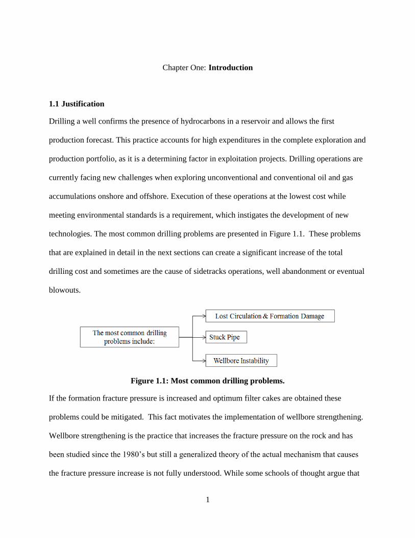
technologies. The most common drilling problems are presented in Figure 1.1. These problems

that are explained in detail in the next sections can create a significant increase of the total

drilling cost and sometimes are the cause of sidetracks operations, well abandonment or eventual

blowouts.

Figure 1.1: Most common drilling problems.

If the formation fracture pressure is increased and optimum filter cakes are obtained these

problems could be mitigated. This fact motivates the implementation of wellbore strengthening.

Wellbore strengthening is the practice that increases the fracture pressure on the rock and has

been studied since the 1980’s but still a generalized theory of the actual mechanism that causes

the fracture pressure increase is not fully understood. While some schools of thought argue that

2

this phenomenon is only possible in permeable formations, others believe that this can even take

place in impermeable formations. At this instance some questions arise related to wellbore

strengthening: what is the predominant mechanism? Can wellbore strengthening take place in

shale cores? Can NPs serve as a wellbore strengthening agent? If so, what would be the wellbore

strengthening mechanism in presence of NPs? What type of NPs are the best? Is there any

optimum concentration of NPs for this purpose? Is there a relationship between wellbore

strengthening and mud filtration? Can NPs also work in recycled mud samples that contain

higher water content and drill cuttings? Can NPs addition result in thinner filter cakes? All these

questions justified the conduction of this research.

1.2 Research Objectives

This dissertation proposes an original research work focused in the application of in-house

prepared NPs for wellbore strengthening and mud filtration reduction. Graphite was added to the

blends as a conventional lost circulation material (LCM). The main objectives of this work are:

Investigate the use of iron-based (NP1) and calcium-based (NP2) as a fluid control

additive at HPHT and LPLT:

- Develop an effective in-situ NPs preparation protocol

- Quantify the mud filtration reduction from NP1 and NP2 at HPHT and LPLT

- Establish the maximum NPs concentration limits in blends

- Determine the filtration reduction trends as a function of NPs and graphite

concentration at HPHT and LPLT

- Establish the optimum concentration of NPs for filtration reduction at HPHT and

LPLT

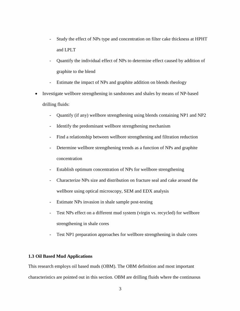
3

- Study the effect of NPs type and concentration on filter cake thickness at HPHT

and LPLT

- Quantify the individual effect of NPs to determine effect caused by addition of

graphite to the blend

- Estimate the impact of NPs and graphite addition on blends rheology

Investigate wellbore strengthening in sandstones and shales by means of NP-based

drilling fluids:

- Quantify (if any) wellbore strengthening using blends containing NP1 and NP2

- Identify the predominant wellbore strengthening mechanism

- Find a relationship between wellbore strengthening and filtration reduction

- Determine wellbore strengthening trends as a function of NPs and graphite

concentration

- Establish optimum concentration of NPs for wellbore strengthening

- Characterize NPs size and distribution on fracture seal and cake around the

wellbore using optical microscopy, SEM and EDX analysis

- Estimate NPs invasion in shale sample post-testing

- Test NPs effect on a different mud system (virgin vs. recycled) for wellbore

strengthening in shale cores

- Test NP1 preparation approaches for wellbore strengthening in shale cores

1.3 Oil Based Mud Applications

This research employs oil based muds (OBM). The OBM definition and most important

characteristics are pointed out in this section. OBM are drilling fluids where the continuous

4

phase is composed of liquid hydrocarbon (Aston, et al. 2002; Bourgoyne et al., 1986). Diesel is

typically used as the constitutive phase because of its viscosity characteristics, low flammability

and low solvency for rubber. The water present in OBM is forming emulsions and for such

phenomenon to take place, a chemical emulsifier must be added to prevent coalescing and

separation of the aqueous phase. Moreover, emulsifiers in the mud also help emulsifying connate

water originally existing in the formation and attached to the drill cuttings. A chemical

wettability agent is also added to make the solids in the mud preferentially oil wet. A schematic

of a stable emulsion is presented in Figure 1.2. The advantages and disadvantages of the OBM

(or diesel based muds) are presented in Table 1-1.

Figure 1.2: Schematic of a stable emulsion (M-I Swaco drilling fluid manual).

The main applications of OBM include (Potma and Drinkwater, 1990; Bourgoyne et al., 1986):

Drilling deep hot formations (T>148°C)

Drilling salt, anhydrite, carnallite, potash or active shale formations

Drilling formations containing H2S or CO2

Drilling of directional or slim holes

Drilling abnormal sub-pressured formations

Drilling while maintaining good corrosion control

5

Table 1-1: Advantages and disadvantages of OBM (Bourgoyne et al., 1986).

Mineral based muds are sometimes applied to mitigate the environmental footprint created by

OBM. This type of mud is an invert emulsion with a continuous specially refined paraffinic-

based oil phase, emulsifiers, dispersants, organophilic clays, calcium oxide or hydroxide, high-

temperature stabilizer and water (Bennett, 1984). Mineral based muds have the same

characteristics of diesel base oils but strong advantages in terms of toxicity (Hinds et al., 1983;

Hinds et al., 1986), and less oil retention have been reported (Bennett, 1984). Another advantage

corresponds to low aromatic exposure to workers and environment (Jacques et al., 1992).

Government Agencies in both the U.S. and U.K. have agreed on the use of mineral base muds in

offshore wells without a cuttings washer as long as a water spray and flume- type oil recovery

facility are used according to the U.S. Mineral Management Services (MMS) (Bennett, 1984).

Mineral base oils are considered low-viscosity/low-colloid oil base fluids where in high

temperature and pressure fluid loss characteristics can be controlled to offer high filtrate (20-40

ml) or a very low filtrate (2-15 ml) (Bennett, 1984).

6

1.4 Common Drilling Challenges

As indicated earlier, common drilling challenges include lost circulation, stuck pipe and wellbore

instability. A description of the most important aspects for each of these challenges is presented

as follows.

1.4.1 Lost circulation

Lost circulation is defined as losses of whole mud to subsurface formations. This can also be

called lost returns. Lost circulation has been one of the main causes for increased drilling costs.

Some drilling problems that are triggered by lost circulation include wellbore instability, stuck

pipe, and eventual blowouts. Lost circulation can occur as (M-I Swaco drilling fluid manual):

Invasion: (or mud loss) to formations that are cavernous, fractured, vugular, or

unconsolidated

Fracturing: mud loss due to presence of fractures created when the wellbore pressure

exceeds the fracture pressure of the rock

Figure 1.3 presents the conditions in which mud losses occur. Lost circulation treatments can be

divided as corrective and preventive. Corrective methods are applied after the occurrence of the

losses (Arunesh et al., 2011). In this condition, lost circulation treatments are either added

continuously to the drilling fluid or spotted as a concentrated pill to mitigate the losses.

The treatment type depends on the degree of losses experienced. For example, settable pills are

used for severe losses. These pills act as cement plugs, gunk, deformable or soft plugs.

Deformable, viscous, and cohesive plugs (DVC) are effective due to their cohesion is able to

create an impermeable seal. For high permeability formation, high fluid-loss high solid-content

squeeze pills are used to mitigate the losses (Wang et al., 2008).

7

Figure 1.3: Sensitive formations for mud losses (Alsaba et al., 2014).

Preventive methods are defined as treatments applied prior to entering lost circulation zones. The

basic principle of these methods is to strengthen the formation (Witfill, 2008). The industry

focuses on different approaches to strengthen the formation. The most accepted approach

consists of propping and sealing the fractures using lost circulation materials (LCMs) (Dupriest,

2005). Propping of the fracture mouth (Alberty and Mclean, 2004), sealing of wellbore by filter

cake (Detournay, 1986; Haimison, 1968) and other methods that also include thermal effects are

believed to serve as a preventive method for lost circulation. However, these have not proven to

be successful in field applications. A detailed explanation of each of these approaches is

presented in the next chapter that is focused on wellbore strengthening.

LCMs are used to stop or mitigate the lost circulation. A current classification of the LCMs was

carried out by Alsaba et al. (2014). Physical and chemical properties are the basis of the next

classification:

8

Granular: are capable of forming seal at the formation face or within the fracture

(Howard et al., 1951; Nayberg et al., 1986). Granular materials include graphite, calcium

carbonate, perlite, asphalt, and nut shell

Fibrous: long, slender, and flexible materials. They may have a little degree of stiffness

and form a mat-like bridge when used in fractured and vugular formations (Howard et al.,

1951). Fibrous materials include cellulose fibers, bagasse, nylon fibers, and mineral

fibers

Flaky: (or lamellated) are thin and flat materials with a large surface area. This material is

able to form a mat over permeable formations. Flaky materials include cellophane, mica,

cottonseed hulls, vermiculite, and flaked calcium carbonate

Mixture of LCMs: mixing of two or more types of the previous mentioned LCM types

showed a better performance due to different particle sizes (Nayberg et al., 1986). The

particle size distribution should be designed carefully. Improper particle size distribution

could result in a poor performance (Alsaba et al., 2014)

Reservoir friendly (acid soluble/water soluble): in comparison to conventional LCMs,

which can cause some formation damage, reservoir friendly LCMs are non-damaging

additives to the reservoir. Acid soluble materials include calcium carbonate and mineral

fibers. Water soluble LCMs include sized salts

Formation damage results from fluid invasion and is an aspect considered during drilling to

ensure an effective well completion (Ghalambor and Economides, 2002). It impacts on well

productivity and injectivity (Bryne and Rojas, 2013) and needs to be mitigated for the

conduction of a successful exploitation project.

9

This phenomenon can occur due to either particle invasion, fines migration to the porous media,

chemical precipitation, organic deposition, or pore collapse (Liu and Civan, 1994). Classic

laboratory studies on formation damage (Mungan, 1965; Gray and Rex, 1966; Muecke, 1979)

concluded that particle transport, formation fines relocation and inorganic and organic

precipitation are the most influential aspects in permeability reduction in consolidated

formations. A later study (Liu and Civan, 1994) proposed a computer tool to study the process of

formation damage focusing on macroscopic and network models. However, this work assumes

an idealized wellbore, linear filtration and analysis of formation damage in laboratory which was

difficult and led to limitations in the results analysis. Presently, industry is focused on new

technologies for formation damage mitigation by preventing fluid invasion towards the porous

media. For example, NPs have been recently used for such purpose (Cai et al., 2012; Zakaria et

al., 2012; Srivatsa et al., 2011; Javeri et al., 2011; Sensoy et al., 2009).

1.4.2 Stuck pipe

Stuck pipe is commonly experienced and can cause serious drilling problems (Muqeem et al.,

2012; Segura, 2011; Yarim, et al., 2007). It can range from a minor to severe stuck. Severe stuck

can eventually result in a sidetrack operation. The drill string gets stuck either by mechanical or

differential effects (M-I Swaco drilling fluid manual).

Mechanical sticking is due to physical obstruction or restriction. Differential sticking is caused

by differential pressures from overbalanced mud columns acting on the drill string against the

filter cake in the wellbore.

Mechanical stuck pipe is divided into two major categories as shown in Figure 1.4:

10

Figure 1.4: Mechanical stuck pipe (modified from M-I Swaco drilling fluid manual).

If drilling is conducted with inefficient well cleaning cuttings are not properly removed from the

bottom of the well causing ‘packoff’ as illustrated in Figure 1.5. In this case the packoff occurred

around the bottom-hole assembly (BHA).

Figure 1.5: Cuttings settlement and stuck pipe (M-I Swaco drilling fluid manual).

Differential stuck pipe occurs due to the following causes:

High overbalance pressures

Thick filter cakes

High-solids muds

11

High-density muds

Figure 1.6 describes the differential sticking. On the left picture the drill collars are centered in

the hole with a mud overbalance. In here the hydrostatic pressure acts equally in all directions.

On the right picture, the collars are in contact with the filter cake. The hydrostatic pressure now

pushes the collars against the wellbore.

Figure 1.6: Mechanics of differential sticking (M-I Swaco drilling fluid manual).

Stuck pipe is solved by jarring down with drill string jars while applying torque. Spotting fluids

can also be used by displacing the annular from the bit to the free point. To prevent stuck pipe

one of the main studies should be focused on obtaining thinner mud cake. New technologies are

currently focused on designing special mud additives to create this effect.

1.4.3 Wellbore instability

Unscheduled events due to wellbore instability accounts for more than 10% of the total drilling

costs which means over $1 billion as a global annual cost. Well instability is caused by (M-I

Swaco drilling fluid manual):

12

Mechanical stress:

o Tension failure – fracturing and lost circulation

o Compression failure spalling and collapse or plastic flow

o Abrasion impact

Chemical interactions with the drilling fluid:

o Shale hydration, swelling and dispersion

o Dissolution of soluble formations

Physical interactions with the drilling fluid:

o Erosion

o Wetting along pre-existing fractures (brittle shale)

o Fluid invasion – pressure transmission

In terms of mechanical stress failure, drilling a stable well requires following an optimum mud

program. An optimum mud program is the one that keeps a mud weight value higher than the

formation pore pressure (to avoid gas kicks or compressive failure) and at the same time less

than the formation fracture pressure (to avoid tensile failure). In conservative models, the

minimum horizontal stress is typically considered as the maximum pressure bound. Figure 1.7

illustrates the consequences of tensile and compressive failure in a well. Compression failure

involves the formation of breakouts on the wellbore in the minimum horizontal stress direction

as shown in Figure 1.8. The breakout angle should be <60° to keep a stable well (Zoback, 2007).

The compressive failure can be modelled using the classic Mohr-Coulomb criterion. Other rock

strength criteria include Hoek and Brown (1980), Modified Wiebols and Cook (1968), Modified

Lade (1977), and Drucker-Prager (1952).

13

Figure 1.7: Results of wellbore instabilities (M-I Swaco drilling fluid manual).

The magnitude of the minimum horizontal stress can be determined based on the extended leak-

off tests (XLOT). This test is typically run in the 10-20 ft interval after the casing is run and

cemented.

Figure 1.8: Wellbore breakout (modified from Zoback, 2007).

14

Figure 1.9 shows a XLOT plot. The most important points of the curve are described on the right

hand side part of the plot. The point at which the curve deviates from its linear behavior is called

the leak-off point (LOP). At this point a hydraulic fracture must be formed. If the LOP is not

reached, a limited test or limited pressure (LP) test is said to be conducted. The formation

breakdown pressure (FBP) indicates unstable fracture propagation. If the pumps continue

operating at a constant rate, a fracture propagation pressure (FPP) is achieved. This is the

pressure that the fracture requires to propagate away from wellbore. If the flow rate and fluid

viscosity are low, FPP could serve as an indicator of the minimum horizontal stress (Zoback,

2007). However, a better estimate of the minimum horizontal stress is carried out by estimation

of the instantaneous shut-in pressure (ISIP). This pressure is measured after an abrupt flow rate

stop and viscous forces becomes negligible. When significant viscous fluids are used or proppant

is involved in the injection, FPP will reach high values due to friction losses. In this case, the

best estimation of the minimum horizontal stress is conducted by measuring the fracture closure

pressure (FCP) (Zoback, 2007). FCP can be calculated by plotting pressure vs. square root of

time and detecting the deviation from the linear performance (Nolte and Economides, 1989).

1.5 Nanoparticles Applications in Drilling Industry

Particles used in drilling fluids with a size between 1-100 nm are called nanoparticles (NPs)

(Amanullah and Al-Tahini, 2009; Zakaria et al., 2012; Hoelscher et al., 2012). The application of

this type of particles in the petroleum industry has become significantly popular in different

disciplines and is capturing the attention of operator companies.

15

Figure 1.9: Schematic of a XLOT (Tutuncu, 2010).

Applications in wellbore strengthening, mud filtrate control as it was previously mentioned (Cai

et al., 2012; Zakaria et al., 2012; Srivatsa et al., 2011; Javeri et al., 2011; Sensoy et al., 2009),

wellbore stability (Riley et al., 2012; Li et al., 2012; Hoelscher et al., 2012), torque and drag

(Hareland et al., 2012), mitigation of pipe sticking (Javeri et al., 2011), and drilling and

production into HPHT conditions (Singh and Ahmed, 2010; Nguyen et al., 2012) are some of the

situations where NPs play a crucial role. These very small particles can have access to the

smallest pores and pore throats acting as a sealing agent in all lithology types including

unconsolidated formations. Due to its ability to form thin, non-erodible and impermeable filter

cake, NPs have demonstrated to be a powerful tool in reducing mud filtrate.

Figure 1.10 shows the NPs effect on mud filtration reduction. These small particles fill the gaps

between the bigger particles creating an effective seal that prevent the mud filtration and

therefore formation damage is mitigated. Note in the picture on the right there is considerably

16

less invasion of particles into the porous media due to the NPs presence forming a seal in the

mud cake, compared to the picture on the left.

Figure 1.10: Effect of NPs in reducing mud filtration towards the formation.

The area to volume ratio is believed to be another reason for the effectiveness of these particles

as it may provide better fluid properties at low concentrations of additives (Amanullah and Al-

Abdullatif, 2010), and the rise of sponge-like clustering behavior which finds applications in

completion fluids (Amanullah and Al-Tahini, 2009). Figure 1.11 shows a plot of surface area to

volume ratio for three different sizes of particles (Amanullah and Al-Tahini, 2009). Other virtues

of NPs correspond to hydrodynamic properties, interaction potential with the formation (Abdo

and Haneef, 2010; Amanullah et al., 2011; Srivatsa, 2010), and improved thermal conductivity

generating low environmental impact as typically the amounts implemented are lower than the

commonly applied mud additives.

17

Figure 1.11: Area to volume ratio of three different sizes of particles (Amanullah and Al-

Tahini, 2009).

In terms of mud filtration reduction, nanoparticles can reach more than 70% of filtrate reduction

in comparison to 9% obtained by common LCM (Zakaria et al., 2012).

Silica nanoparticles are implemented for reducing shale permeability and therefore ensuring the

well stability through these formations by avoiding the use of water based muds (WBM). Figure

1.12 presents a cryo Transmission Electron Microscope (TEM) of two different nanosilica

particles with the same particle size but different stabilization/suspension packages; one having a

more resilient aspect that can be useful when contacting the pore space (Riley et al., 2012).

Figure 1.12: Arrangement of nanosilica particles of 20 nm mean diameter viewed under the

TEM (Riley et al., 2012).

18

Current advances in nanoparticles technology have allowed improvement in wellbore stability

while drilling by shale stabilization by plugging its nanometer-sized pores (Hoelscher et al.,

2012; Friedheim et al., 2012) using the Shale Membrane Tester (SMT) operated by the

University of Texas at Austin and M-I Swaco on Marcellous and Mancos shales in the presence

of WBM. The experimental set-up includes placing a shale core (well-preserved) into a cell

under differential pressure applied on both sides of the sample. The operating principle consists

of calculating the speed at which the top and bottom pressures become the same by fluid flowing

through the shale from the top to obtain permeability. From this experiment it was found initially

that silica NPs of 10 wt% were needed to significantly reduce the shale permeability. Since it

was a considerably high concentration that would involve high operational costs, screening tests

were performed to reduce this concentration up to 3 wt% obtaining a permeability reduction

around 98%.

1.6 Dissertation Chapters Description

This Dissertation is divided into six chapters that cover the analysis of wellbore strengthening

and mud filtration control by means of in-house prepared NP-based drilling fluids for sandstone

and shale formations.

Chapter 1 (this chapter) is an introduction to the work that justifies the research performed, states

the research objectives, describes applications of OBM, and explains common drilling challenges

sensitive to improvement from this research results. NPs applications in drilling industry were

discussed, and virtues of the NPs were highlighted.

Chapter 2 focuses on wellbore strengthening. As a motivation, the wellbore strengthening impact

in Western Canada was quantified from a technical and economical point of view with a case

19

study that involved drilling and completion data from two wells. A literature review on wellbore

strengthening was conducted including the most influential theories that explain the mechanism.

Understanding the implications of each mechanism played a crucial role in the development of

this research.

Chapter 3 presents an original NPs application for mud filtration control at HPHT and LPLT.

Successful application of in-house prepared NPs to reduce mud filtration was experimentally

quantified at different temperature and pressure conditions. Ceramic discs of low permeability

were used to simulate a porous media. NPs were prepared within OBM with presence of

graphite. Filtration reductions up to 76% were achieved at HPHT and reductions up to 100%

were achieved at LPLT.

Chapter 4 describes an original research for wellbore strengthening in sandstone cores. OBM

with presence of NPs and graphite achieved up to 65% of fracture pressure increase. Strong

match between wellbore strengthening and filtration at HPHT was discovered. Wellbore

strengthening trends as a function of NPs concentrations were established and optimum NPs

concentration identified. The wellbore strengthening mechanism was investigated and described.

Optical microscopy, SEM, and EDX analysis were conducted on cores post-testing to infer about

the predominant wellbore strengthening mechanism. NPs presence on the seal developed along

the fracture and filter cake around the wellbore was characterized.

Chapter 5 presents original research for wellbore strengthening in shale cores. Contrary to the

common belief in industry that wellbore strengthening cannot be achieved in shale formations,

this chapter demonstrates that wellbore strengthening can be achieved in shale cores based on

experimental evidence using nanoparticle-based drilling fluids. Fracture pressure increase up to

30% was achieved. Wellbore strengthening trends as a function of NPs concentration were found

20

and optimum concentrations determined. Shale pore throat modeling, Optical microscope, SEM,

and EDX analysis were carried out in shale samples post-testing and concluded that tip resistance

by a seal formed along the fracture was the wellbore strengthening mechanism. NPs presence in

the seal along the fracture was characterized.

1.7 Technical Publications

The technical papers that resulted from this research and have already been accepted for

presentation are listed below:

Contreras, O., Hareland, G., Husein, M., Nygaard, R., and Alsaba, M. 2014. Application

of In-House Prepared Nanoparticles as a Filtration Control Additive to Reduce Formation

Damage. SPE paper 168116 prepared for presentation at the SPE International

Symposium and Exhibition on Formation Damage Control held in Lafayette, LA, USA,

26-28 Feb (Currently under peer-review at the JCPT)

Contreras, O., Hareland, G., Husein, M., Nygaard, R., and Alsaba, M. 2014. Wellbore

Strengthening in Sandstones by Means of Nanoparticle-Based Drilling Fluids. SPE paper

170263 prepared for presentation at the SPE 2014 Deepwater Drilling and Completions

Conference held in Galveston, TX, USA, 10-11 September

Contreras, O., Hareland, G., Husein, M., Nygaard, R., and Alsaba, M. 2014.

Experimental Investigation on Wellbore Strengthening In Shales By Means of

Nanoparticle-Based Drilling Fluids. SPE paper 170589 prepared for presentation at the

2014 SPE Annual Technical Conference and Exhibition held in Amsterdam, The

Netherlands, 27-29 October

21

Contreras, O., Alsaba, M., Nygaard, R., and Hareland, G. 2014. Review of Lost

Circulation Materials and Treatments with an Updated Classification. AADE-14-FTCE-

25 paper prepared for presentation at the American Association of Drilling Engineers

(AADE) 2014 National Technical Conference and Exhibition held in Houston, TX, USA,

15-16 April

22

Wellbore Strengthening Chapter Two:

2.1 Introduction to Wellbore Strengthening

Wellbore strengthening is defined as the practice of increasing the fracture gradient in a

determined well section. As mentioned earlier, this practice can have multiple applications in oil

and gas exploitation projects. From a practical perspective, wellbore strengthening can widen the

mud operational window. The mud operational window defines the minimum and maximum

mud weight bounds during drilling operations. As mentioned in the previous chapter, for a stable

drilling operation, the mud weight should not be lower than the pore pressure and/or collapse

pressure. Also, mud weight cannot exceed the fracture gradient since a tensile fracture will be

created and mud losses will occur. Figure 2.1 shows a schematic of an original mud window that

got narrowed due to two different operational conditions. If an offshore well experiences an

increase of the water depth, a reduction in fracture gradient will occur due to a less compaction

of the sediments. Also, the lower limit might be increased due to an increase in collapse pressure

of weaker formations. Another scenario involving narrowing of the mud window occurs in

deviated or horizontal wellbores as illustrated in the right hand plot. If a horizontal well is drilled

in an isotropic stress conditions the fracture gradient of the deviated section is lower than the

fracture gradient for the vertical section (Salehi, 2011).

Considering that the in-situ stresses act in a determined volume of earth crust as illustrated in

Figure 2.2, the overburden stress can be defined as Eq. 2.1 where g is gravity, is formation

density and z is depth (Salehi, 2011):

z

v dzg0

Eq. 2.1

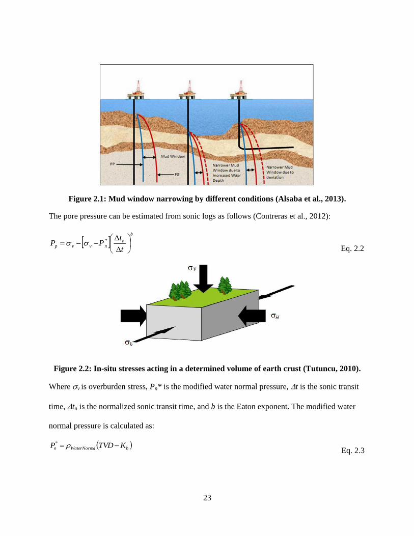
23

Figure 2.1: Mud window narrowing by different conditions (Alsaba et al., 2013).

The pore pressure can be estimated from sonic logs as follows (Contreras et al., 2012):

b

nnvvp

t

tPP

*

Eq. 2.2

Figure 2.2: In-situ stresses acting in a determined volume of earth crust (Tutuncu, 2010).

Where v is overburden stress, Pn* is the modified water normal pressure, t is the sonic transit

time, tn is the normalized sonic transit time, and b is the Eaton exponent. The modified water

normal pressure is calculated as:

blWaterNorman KTVDP *

Eq. 2.3

24

The tensile failure criterion states that a fracture will initiate when (Fjaer, 2008):

oT Eq. 2.4

Where is the tangential (hoop) stress around the wellbore and To is the tensile strength of the

formation. For vertical and circular wellbore, without presence of natural fractures and fluid

invasion, the fracture breakdown pressure (Pfb) is defined as:

poHhfb PTP 3 Eq. 2.5

Fracture gradient is estimated by dividing Pfb by an specific depth. The fracture breakdown

pressure for deviated wellbores can be calculated in function of the Pfb for vertical wellbores as

(Aadnoy and Chenevert, 1987):

sin163

1 pfbdeviatedfb PPP

Eq. 2.6

Where is the wellbore inclination. The collapse pressure can be estimated as (Fjaer et al., 1992):

1*tan

22

*

UCSP h

w Eq. 2.7

Where UCS stands for the unconfined compressive strength and half of the Mohr failure

angle. If wellbore strengthening is achieved, a safer drilling operation could be conducted since

the mud program will allow a broader range of values. The way in which wellbore strengthening

can be achieved is still a subject of discussion. Types of formation in which wellbore

strengthening can happen is still not established and the optimum type of particles or mud

additives has not been addressed explicitly on a uniform theory. Motivation on the

implementation of wellbore strengthening in Western Canada is presented next. Then, a literature

review on the wellbore strengthening mechanisms is conducted.

25

2.2 Motivation: Potential Impact of Wellbore Strengthening in Western Canada

Drilling operations in the prolific Western Canada Sedimentary Basin (WCSB) is a routine

practice that typically consists of empirical practices. This basin contains giant tight sands and

shale gas reservoirs that are currently exploited by a variety of operators. The aim is to drill and

complete the wells in less time while maintaining environmental regulations. However, drilling

optimization is not typically conducted and this impedes an efficient drilling and completions

operations. Reduction in numbers of casings runs into a well would significantly affect the

completions plan and therefore the total expenditures.

A quantitative analysis of wellbore strengthening in reducing the number of casing strings is not

widely reported in the literature. This motivated the endeavor of developing a quantitative

analysis of this fact. By quantifying the effect of wellbore strengthening on reducing the number

of casing strings in two vertical wells A and B, the technical and the economic advantage can be

identified and quantified. The two wells analyzed in this study were drilled in the Deep Basin of

the WCSB to contact a gas reservoir into a prolific continuous gas accumulation. A map that

highlights the study area is presented in Figure 2.3. Both wells were drilled in 2007 and the

authorizations for expenditures (AFE) were available (Contreras, 2011). The drilling and

completion costs may be currently different for wells drilled in this area; however, the analysis

was based on percentage of cost reductions that allows a fair study and discussion.

One of the main challenges of this study relates to the very limited wellbore strengthening data

collected for the different formations in order to be able to address the application in a complete

well section.

26

Figure 2.3: Deep Basin of the WCSB (modified from Masters, 1984).

Obtaining this data through tests involving the hydraulic fracturing apparatus takes a

considerable amount of time and carries significant expenditures. Because of this limitation, it

would be considered in this analysis that all the sandstone formations along the two wells can be

strengthened up to 42.8% in the presence of the blend containing NPs and glide graphite. The

strengthening of the shale formations will be considered of 18.6%. These average values

correspond to the final results obtained from this research which will be discussed in Chapters 4

and 5. Discretization between sandstones and shaly formations was performed using a V-shale

cut-off of 0.6 as suggested by Contreras (2011) in this area. An analysis on the complete well

sections and quantification of the number of casing runs that could be reduced using an

optimized blend in presence of NPs and LCM will be studied from a technical and economic

perspective.

2.2.1 Technical analysis

Application in well A

Well A is a vertical well with total depth of 3252 m. A surface casing was set at 606.93 m by the

operator. Until this depth the well was drilled using WBM. From this depth on, three casing

27

strings are needed to ensure wellbore stability considering the mud window between the pore

pressure gradient and fracture gradient according to the Bourgoyne et al. (1986) analysis as

presented in Figure 2.4a. The mud window was developed based on the mathematical models

presented in the previous section. The design principle is not to go below the pore pressure

gradient since a gas influx can be experienced and at the same time stay below the fracture

gradient in order to avoid formation fracturing and, consequently, mud losses. In this figure, the

pore pressure gradient is presented as a blue profile and the fracture gradient as a green profile.

The two red lines account for an average value of pore pressure gradient and fracture gradient.

The number of casings needed is represented by the yellow vertical lines. Note that only values

are plotted from 586 m on, as this is the starting depth of availability of well logs used in the

study. If wellbore strengthening is achieved in the percentages previously mentioned, the fracture

gradient is increased and therefore the green profile will move to the right as presented in Figure

2.4b. Under this scenario, just two casing runs are needed from surface casing to final depth

avoiding the casing run from 2500 m to 3000 m.

Application in well B

Well B is a vertical well of total depth of 3212 m and where the surface casing was set at 610 m.

from this depth, two casing strings are needed to ensure well stability through an analysis similar

to that performed in well A. The number of casing strings required is presented in Figure 2.5a.

If wellbore strengthening is achieved as in well A, just one casing string is needed from surface

casing to the final depth as presented in Figure 2.5b. This is a quite remarkable result that

indicates that in the study area mono-bore wells could be drilled which in turn will significantly

reduce the completion expenditures.

28

(a) (b)

Figure 2.4: (a) Mud window for well A and definition of casing setting depths. Red profiles


window for well A and definition of casing setting depths after wellbore strengthening. Red

profiles correspond to average values of pore pressure gradient and fracture gradient.

(a) (b)

Figure 2.5: (a) Mud window for well B and definition of casing setting depths. Red profiles


window for well B and definition of casing setting depths after wellbore strengthening. Red

profiles correspond to average values of pore pressure gradient and fracture gradient.

29

2.2.2 Economic impact

The economic impact of the technical analysis is considered based on the AFE of wells A and B.

These wells were drilled in the same drilling campaign and the costs of casing strings, casing

attachments and cementing is essentially the same. According to the AFE, the total cost for a

surface casing and attachments is $63,250. The cementing of the surface casing is $18,360. The

cost for each intermediate casing and attachments is $70,530 and the cementing cost for the

intermediate casing is $24,280. In terms of casing strings and completion, the well A will require

for its conventional completion a total number of four casings (including casing attachments and

cement) for a total amount of $366,040.

If wellbore strengthening is achieved by using and NPs and LCM blend as presented in previous

analysis so that one casing run can be avoided, the total cost will decrease to $271,230. This

means a cost reduction of 25.9% for casing runs (including attachments) and cementing. In

addition, there are large savings in costs related to drilling and tripping time by eliminating one

casing string as well as less bits needed and better ROP optimization resulting in lower overall

$/m. Table 2-1 shows the costs associated to the time spent on casing running. Summation of all

the parameters gives a spread rate of 1,457.29 $/hour. The casing running and cementing

operations in this wells takes a total of 24 hours according to the daily drilling reports. This

means an additional cost saving of $34,968.

30

Table 2-1: Drilling costs for well A from AFE.

Well B requires for its conventional completion three casing strings (including casing

attachments and cement) for a cost of $271,230. If wellbore strengthening can reduce one casing

string as analyzed previously, the cost will decrease to $176,420 implying a cost reduction of

34.9%. On the other hand, if well B is decided to be run as a mono-bore, the cost will be

significantly reduced as only one casing string will be required. Table 2-2 shows the costs for

well B. Summation of all the parameters gives a spread rate of 1,659.37$/hour. The casing

running and cementing of this well takes a total of 24 hours giving this an additional saving of

$39,824.

31

The average value of drilling and abandonment of each well lays on $2,300,000 based on the

AFEs. If wellbore strengthening is achieved in both wells, a cost reduction based on the total

drilling and abandonment cost of 5.64% and 5.85% can be obtained in wells A and B

respectively. If we consider that a drilling campaign in western Canada involves drilling of 45-80

wells/year, these costs savings become much more significant.

Table 2-2: Drilling costs for well B from AFE.

32

2.3 Literature Review on Wellbore Strengthening Methods

Wellbore strengthening was studied experimentally in the 1980s by the DEA-13 project (Morita

et al., 1990; Fuh et al., 1992). Later, the GPRI joint industry project (Van Oort and Friedheim,

2011; Dudley et al., 2001) was accomplished trying to replicate the DEA-13 experimental work

in a smaller scale. From these studies the first insights for the wellbore strengthening mechanism

were pointed out and served as the basis of the current school of thought that tries to explain the

mechanism. Currently, the drilling industry is focused mainly on two mechanisms: tip resistance

by the development of an immobile mass (Dupriest, 2005) and stress caging theory (Alberty and

Mclean, 2004). Another approach called “fracture propagation resistance” was presented by

(Van Oort and Friedheim, 2011) which is built in basic principles of the DEA-13 and GPRI

projects. A recent study (Salehi, 2011) performed a numerical simulation of fracture propagation

and sealing on the wellbore and their implications in wellbore strengthening. Mostafavi (2011)

developed an experimental analysis and mechanistic modeling of wellbore strengthening. Later,

Nwaoji (2012) performed experimental research on wellbore strengthening involving ex-situ

prepared nanoparticles mainly in WBM systems. Additional analysis that involved elastic-plastic

fracture models, boundary elements, filter-cake bridging and thermal effects haven also been

presented. The key points in each of these studies will be presented as follow.

2.3.1 DEA-13 project

One of the first published works for understanding the wellbore strengthening mechanism

corresponded to the DEA-13 project (Morita et al., 1990; Fuh et al., 1992). Different fluids and

concentrations were tested for fracturing tests and fluid loss measurements. Reopening pressure

was observed to be higher in the presence of WBM as compared to OBM despite experiencing a

similar fracture breakdown pressure as illustrated in Figure 2.6. This phenomenon was explained

33

by the effect of the filter cake and amount of filtrate into the formation. In addition, they

mentioned the feasibility of the tip screen out as the governing mechanism of the wellbore

strengthening, in which particles form a filter cake inside the fracture and the wellbore pressure

is no longer transmitted to the fracture tip as it is screened out. This indicates that fracture sealing

by development of an immobile mass was the governing mechanism. Figure 2.7 shows a rock

sample post-testing along the fracture plane. A non-invaded, mud dehydrated zone and fractured

zone were three distinctive zones observed.

Figure 2.6: Similar initial fracture breakdown pressure using water and oil-based muds

(Morita et al., 1996).

DEA-13 also mentioned the occurrence of peak shapes in the pressure behavior versus time

when utilizing WBM. They believed that the screen out generated a complete fracture sealing

requiring a higher pressure level to go through to the current fracture tip. It was also stated that

more unstable fracture propagation took place on low permeability formations due to weak filter

cakes created.

34

Figure 2.7: Core after hydraulic fracturing experiment (Wang, 2007).

2.3.2 GPRI Joint Industry Project (JIP)

GPRI project was conducted in late 1990s to replicate and corroborate results from DEA-13

project in a less-cost smaller scale (Van Oort and Friedheim, 2011; Dudley et al., 2001). LCM’s

effect on fracture pressure was studied. From the study, synthetic graphite of specific types and

sizes was able to significantly enhance the fracture pressure. This material was able to enter and

seal the fracture. WBM were found to provide superior performance in comparison to synthetic-

based muds (SBM). A screening on different wellbore strengthening materials was conducted on

SBM and some of them were able to raise the fracture propagation pressure. Re-opening pressure

as a function of hydraulically conductive fractures was also quantified in these experiments. The

ideal fracture re-opening pressure can be lowered by hydraulic conductive fractures close to the

confining pressure or minimum horizontal stress.

2.3.3 Stress caging theory

The stress caging theory has been studied by different researchers (Wang et al., 2009; Wang et

al., 2008; Soroush and Sampaio, 2006; Song and Rojas, 2006; Aston et al., 2004; Alberty and

McLean, 2004). The fundamental principle of the stress caging corresponds to the deposit of

solids at or close to the fracture mouth to act as both proppant and seal isolating the fluid

pressure. Considering a sufficient permeable formation, the filtrate beyond the blockage will

35

dissipate and pressure in the isolated part of the fracture will eventually reach the same value of

the formation pressure (pore pressure) and subsequently the fracture will start to close. An

increase in hoop stress is generated by the fracture that intends to close compressing the

blockage. Figure 2.8 shows a schematic of the stress caging as a wellbore strengthening

mechanism.

Figure 2.8: Stress caging theory.

Stress caging has also been reported to be the mechanism for wellbore strenghtening in shale

formations (Aston, et al., 2007). This approach is based on the transportation of bridging

particulate media that could act as “cement” into the fracture. The solidification will avoid

seapage and flow back towards the wellbore.

From all the stress caging theory models previously mentioned, a mathematical summary is

developed by the autor in order to capture the physical phenomenon. Assuming that at t=0 the

36

fracture was created, then at t=t1: time at which the fracture is propagating in the far field stress

region (i.e., region with no effect of hoop stress) we have:

Pf1=Pw1, and, P f1>h’+P1 Eq. 2.8

where Pf1 is the pressure of the fluid into the fracture at t=t1, Pw1 is the pressure in the wellbore at

t=t1, h’ is the effective in-situ horizontal stress and P1 is the pore pressure at t=t1. At t=t2: time

at which the fracture stops growing we have:

Pf2<Pw2, and, Pf2=h’+P2 ; (this implies Pf2>P2) Eq. 2.9

where Pf2 is the pressure of the fluid into the fracture at t=t2, Pw2 is the pressure in the wellbore at t=t2,

and P2 is the pore pressure at t=t2. At t=t3: time at which the fracture starts closing we have:

Pf3<<Pw3, and, Pf3<h’+P3; (this implies Pf3=P3) Eq. 2.10

where Pf3 is the pressure of the fluid into the fracture at t=t3, Pw3 is the pressure in the wellbore at

t=t3, and P3 is the pore pressure at t=t3.

Numerical studies (Salehi and Nygaard, 2012; Salehi, 2011) on the stress caging mechanism

showed that wellbore hoop stress after wellbore strengthening did not exceed ideal hoop stress

for the intact wellbore arguing just a fracture gradient restoration. This means that the stress

caging is described as an ideal mechanism that will not take place in real field conditions. Also,

explicit and comprehensive experimental evidence that confirms the occurrence of the stress

caging has not been published up to now (Van oort et al., 2011).

37

2.3.4 Tip Resistance by development of an immobile mass

Dupriest (1995) presented fracture closure stress practices where the fracture was blocked by

particles so that the pressure was not transmitted to the tip. In this instance, the fracture width

plays a crucial role as it might be widen when additional pressure is applied in the wellbore and

the blocking material is bypassed. When the LCM is driven into the fracture, it is believed that

an immobile mass can isolate the fracture tip due to the loss (mud filtrate) of its carrier fluid to

the formation. Initially there is low resistance to flow into the fracture, however if resistance

occurs the back pressure widens the fracture. This elastic growth of fracture width regulates the

build-up pressure. This phenomenon is represented graphically in Figure 2.9. As the fracture is

packed back to the wellbore, higher wellbore pressure values are required to continue the

fracture extension causing wellbore strengthening. Some difficulties in the creation of the

immobile mass by LCM arise when the formation has a too low permeability as the mechanism

requires some leak-off. However, some material can invade induced and widened fractures in

impermeable media.

Figure 2.9: Tip resistance by the development of an immobile mass.

38

This wellbore strengthening mechanism does not require modeling of the LCM strength and

type. This was found as a non-important parameter for the tip isolation.

2.3.5 Sealing of wellbore by filter cake

Sealing the wellbore by creation of an effective filter cake strengthens the wellbore. This

phenomenon is based on the definition of fracture breakdown pressure. The fracture breakdown

pressure (Pfb) for a vertical wellbore was defined in Eq. 2.5 in porous rocks where a filter cake is

present isolating the pressure in the wellbore with the pore pressure (i.e., preventing mud

filtrate). However, when there is no filter cake and mud filtration takes place, the expression

becomes (Detournay, et al., 1986 and Haimison, 1968):

2

23 poHh

fb

PTP Eq. 2.11

where,

)1(2

21

v

v

Eq. 2.12

is the Biot's constant, v is the Poisson’s ratio, and the poro-elastic parameter is always less

than 1.0, which implies a reduction of the fracture breakdown pressure when mud filtration

occurs. Assuming an isotropic stress condition in the horizontal direction, and a negligible

then the expression becomes:

pphfb PPP 12 Eq. 2.13

Rearranging, the next expression is obtained:

'21 hhfb vP Eq. 2.14

According to Wang et al. (2007), if (1-2v)>0 for a sedimentary rock, then Pfb>h. with v=0.25,

39

2

'

hhfbP

Eq. 2.15

When Pp tends to zero, h tends to h’. Therefore Pfb can be much more higher than h. A main

conclusion from this analysis is that Pfb can be reduced due to fluid invasion but at the same time

be higher than h.

2.3.6 Fracture propagation resistance (FPR)

The fracture propagation resistance approach (Van Oort and Friedheim, 2011) is based on the

conceptual basis from DEA-13 and GPRI project. With the implementation of this approach,

mud losses have been reduced in more than 80% in the Gulf of Mexico (GoM) by preventing the

occurrence of induced fractures. In contrast to these analyses, the FPR involves the use of

different types and concentrations of wellbore-strengthening materials (WSMs). The most

important differences between the FPR and the stress caging and fracture tip isolation

mechanism are presented in Table 2-3.

Table 2-3: Differences on techniques for wellbore strengthening.

FPR aims for an increase in fracture propagation pressure. It is based on fracture tip isolation

where WSMs of specific type and size are important. The size of these particles is also

dependent on the mechanical properties of the rock. This approach can be conducted on OBM or

synthetic-based mud while not requiring squeeze operations. The WSMs are always present in

40

the mud, i.e., a pill is not required. FPR is an effective approach to avoid natural or induced

fractures in shale/sands interfaces. The laboratory evaluation of the WSMs was carried out using

a testing device shown in Figure 2.10 that recreates fractures of different width in impermeable

rock. The objective is to test fracture sealing as a function of mud additives.

Figure 2.10: Test apparatus for WSMs screening and selection (Van oort et al., 2011).

Fracture apertures between 300 and 1000 microns were simulated. The most important

characteristic of the WSMs for an effective fracture sealing were the particle size, particle-size

distribution, concentration, shape, surface texture, compressive strength, bulk density and

resiliency. Synthetic graphite, ground nut hulls, and proprietary oil-wet cellulose particles were

encountered as the best performing material from the screening. It is stated in this study that

further work is required to clearly demonstrate increase in fracture initiation and/or reopening

pressures using leak-off tests (LOT).

41

2.3.7 Numerical simulation of fracture propagation and sealing

Salehi (2011) studied the hoop stress effect of wellbore strengthening. Three-dimensional poro-

elastic finite element simulations were conducted to simulate fracture initiation, propagation and

sealing. A methodology for fracture initialization based on non-linear behavior was conducted

using cohesive modeling. This author argues that wellbore strengthening is only able to cause

hoop stress restoration, but it is not able to increase the hoop stress over its ideal or original

maximum value defined by the Kirsch (1898) analytical solution. Figure 2.11 models the shift

from tensile to compressive mode of the hoop stress. However, the hoop stress is not able to

exceed its original value.

Figure 2.11: Hoop stress at wellbore after fracture sealing (black line), fracture

propagation (redline), fracture initiation (green line) and for intact wellbore (blue line)

from Salehi (2011).

Salehi suggested that the LOT interpretations needs to be conducted carefully. Well conditions

for interpretation of LOT in a well are summarized in Figure 2.12. For an intact borehole, the

pressure has to exceed the effective hoop stress and tensile strength. If a small fracture is present,

the tensile strength does not need to be overcome and the fracture will initiate just by reaching

the effective hoop stress. If a large fracture is along the wellbore, the pressure will reach just the

42

minimum horizontal stress value to propagate the fracture. If a long fracture along the wellbore is

intersecting vugs or natural fractures, then maximum pressure reading will be the pore pressure.

Figure 2.12: Wellbore condition in LOT interpretation (Salehi, 2011).

2.3.8 Experimental analysis and mechanistic modeling of wellbore strengthening

A wellbore strengthening mechanism and parameters involved on wellbore strengthening were

analyzed by Mostafavi (2011). Resilient graphite was identified as the material that provides the

best performance for wellbore strengthening from core fracturing and core reopening

experiments. Core fracturing tests were carried out in the experimental facility illustrated in

Figure 2.13 located at the University of Stavanger in Norway. Concrete samples were used in

the experimental testing. The calcium carbonate in fiber and granular forms was found

ineffective in the core fracturing tests.

43

Figure 2.13: Core fracturing system set-up (Mostafavi, 2011).

Analysis of friction coefficient of the fracture plane concluded that the strengthening process is

improved by higher friction coefficients. An analytical model for tensile fractures was developed

in this work. An increase of the initial breakdown pressure can be obtained. The model includes

fracture size distribution, concentration of particles in the drilling fluid, fracture geometry,

mechanical properties of the particles and friction coefficient of the fracture planes. A critical

particles concentration into the drilling fluid was established. Beyond this concentration the

strengthening process is not improved. This work only considered conventional LCM. Also, the

tests were not conducted in real rock samples. This limits the extrapolation from this idealistic

model to real field operations.

2.3.9 Wellbore strengthening-nano-particle drilling fluid experimental design using a

hydraulic fracture apparatus

Nwaoji (2012) did a first attempt for wellbore strengthening using fluids containing NPs and

LCM. Calcium-based and iron-based NPs were prepared ex-situ and tested in water based mud

and oil based mud. Ex-situ NPs preparation stands for the preparation of NPs in an aqueous

media and then mixing with the mud. For practical purposes, this is not an advisable way for NPs

preparation since it will involve an increase of the water content in the mud. A maximum

44

breakdown pressure increase of 70.31% was obtained using WBM in a permeable media. The

WBM tested was not commercial; it was just composed of water and bentonite. OBM was also

involved in the testing and a maximum breakdown pressure increase of 36.39% was achieved.

The wellbore strengthening mechanism was not addressed. Figure 2.14 shows a pressure vs.

time plot for an OBM blend tested in a sandstone core. Blend 8 stands for a blend containing

NP2 and graphite. Blend 3 contains NP1 and graphite. The control sample is just OBM free of

NPs and LCM. The breakdown pressure increase can be observed from the curves with higher

pressure values than the control sample.

Figure 2.14: P vs. t plot for OBM containing NPs tested on sandstone core (Nwaoji, 2012).

Overall, the WBM performed better than the OBM. This is believed to be due to thicker filter

cake formed with WBM that could help for the fracture sealing. Filtration tests in these blends

were not conducted and this was a limitation of this work. Graphite exhibited superior

strengthening characteristics in comparison to the calcium carbonate as the LCM used. However,

blends containing just graphite (with no NPs) were not analyzed to quantify the effect that NPs

have over the LCM. This means that the positive effect (if any) of NPs on wellbore strengthening

was not quantified. Few tests were run in concrete cores simulating an impermeable media and

45

some degree of strengthening was achieved. In this case the blends containing iron NPs

performed better than the calcium NPs. While a concrete core can simulate an impermeable

media, it cannot be compared with a shale formation. Shale formations have much more different

mechanical properties than concrete. Also, shale formations are sensitive to contact with air and

water while the concrete samples are not. Despite the multiple limitations of this work, results

that might be of interest for field applications were pointed out.

2.3.10 Other wellbore strengthening mechanisms

Other wellbore strengthening mechanisms include the elastic-plastic fracture model proposed by

Aadnoy and Belayneh (2004). They experimentally proved that the fracture resistance is

sensitive to mud composition. They explained the pressure increase considering that cake does

not get broken when the fracture is opened, indeed, it deforms plastically by maintaining a

barrier as illustrated in Figure 2.15. This mud cake deformation cannot take place in low-

permeability formations and this was the reason why they did not find a match between the

analytical and laboratory experiments. They recommended the use of materials of high

mechanical strength instead of polymer-based materials. The fracture breakdown pressure

showed to be very sensitive to the particles content as bridging materials.

Figure 2.15: Elastic-plastic borehole fracture model (Aadnoy and Belayneh, 2004).

Additional works on wellbore strengthening are reported in literature with either limited

experimental or field application evidence. These are listed as:

46

Internal filter-cake bridging and time-dependant wellbore strengthening

(Abousoleiman et al., 2007; Reid and Santos, 2006; Santos et al., 2006):

development of an impermeable filter cake formed inside the fracture increases

fracture resistance

Wettability change of filter cake (Brege et al., 2010): changing filter cake

wettability in presence of non-aqueous fluid from oil-wet to water-wet can increase

the fracture healing of the mud

Thermal effects (Gil et al., 2006; Gonzalez et al., 2004): The near wellbore fracture

pressure can be increased by thermal treatments. By increasing mud and wellbore

temperature the effective fracture pressure can be increased and mud losses can be

prevented. Coupling the thermal effects with the stress caging theory has also been

reported. Initially the wellbore is cooled down to reduce the hoop stress. Then the

stress caging procedure is conducted. Once the fracture reached the end of the

“cold” region the fracture is believed to seal. The whole system will be under

compression when it reaches the original wellbore temperature. This is just an ideal

model carried out using finite element models.

2.3.11 Discussion of wellbore strengthening mechanisms

From all the previous wellbore strengthening mechanism discussed, the tip resistance by the

development of an immobile mass and the stress caging theory are the only ones that are

believed to have impact on field operations. These two mechanisms have been proposed based

on utilization of conventional LCM and granular mud additives.

47

Figure 2.16: Contrast between tip resistance by the development of an immobile mass and

stress caging mechanisms.

Figure 2.16 presents a comparison of the pressure behavior from wellbore to the fracture tip

between the tip resistance by the development of an immobile mass and the stress caging

mechanisms. A situation in which no wellbore strengthening effect is reached is also described

as constant pressure behavior. Note that in the fracture tip isolation there is a sudden decrease in

pressure before the fracture tip. This requires a higher pressure applied to widen the fracture and

overcome the seal. For stress caging, there is a pressure reduction just ahead of the fracture

mouth. This pressure occurs due to the isolation of the body of the fracture with the wellbore.

This will eventually cause the fracture closing due to pressure dissipation in the fracture body.

The next chapters will focus on the identification and investigation of the predominant wellbore

strengthening mechanism by using OBM samples containing in-situ prepared NPs.

48

Nanoparticles Application for Mud Filtration Control Chapter Three:

3.1 Introduction to NPs Application for Mud Filtration Control

NPs as a filtration reduction agent is becoming a more popular practice as documented in

Chapter 1. In this research, NPs application for filtration control in OBM was studied for two

different conditions: HPHT and LPLT. Both set of tests followed the API standard procedure and

were conducted at the Drilling Fluids Laboratory of the Missouri University of Science and

Technology. The hypothesis behind this research step is to relate filtration with wellbore

strengthening. While several authors (Song and Rojas, 2006; Dupriest, 2005, Aston et al., 2004;

Alberty and McLean, 2004) argue that some filtration is required for wellbore strengthening to

take place, it is also important to identify the filtration limit that will impair strengthening

performance. High filtration is associated with weak filter cakes that eventually will not

positively impact the strengthening mechanism. NP1 and NP2 were prepared in-situ from

commercial precursors in OBM to simulate a field practice. The OBM used is a commercial fluid

used in western Canada drilling operations and was provided in 4-gallon containers. Mixing of

the OBM itself was required before the NPs preparation, due to sedimentation that occurs if

mixing is not performed. Graphite was used as a conventional LCM at two different

concentrations to help the filtration process. Graphite is also a required additive for wellbore

strengthening, and modeling of the graphite performance in filtration will allow the

establishment of a match between filtration and strengthening as will be addressed in the

upcoming chapter. Since early 90’s, the graphite has been identified as a powerful wellbore

strengthening agent (Morita et al., 1990; Fuh et al., 1992). Current research (Nwaoji, 2012)

49

concluded the superior performance of graphite compared to calcium carbonate in wellbore

strengthening tests using OBM.

From this study filtration performance of NPs was investigated as a function of pressure,

temperature and concentration of additives. Impact in resulting blends-rheology was analyzed as

a consideration for application in field operations. Optimum NPs and graphite concentrations

were identified and the individual effect of NPs and graphite was quantified at such

concentrations. Results indicate that blends containing NPs and LCM behave differently at

different pressure and temperature conditions, always with NP1 giving a superior effect on

filtration reduction.

3.2 Experimental Methods

3.2.1 Drilling fluid characterization

OBM was selected as the drilling fluid in this work. This type of mud is used broadly due to its

inhibitive characteristics while drilling shale formations, low density values for applications in

sub-pressured basins, good rheological properties at high temperatures and superior lubrication

characteristics in comparison with WBM. The composition and rheology of the OBM used in

this study is presented in Table 3-1.

Table 3-1: OBM composition and rheology.

Oil/Water Ratio 90/10

CaCl2 brine (30 wt% solution) 10%

Emulsifier (tall oil fatty acid) 8.0L/m3

Hydrated lime 15-20 kg/m3

Gilsonite 5.0 kg/m3

Organophilic clay 5 kg/m3

Mud rheology

PV=15 cP, YP=4 lb/100ft2, Gel 10s=1.8 lb/100ft2, Gel10min=2 lb/100ft2

50

3.2.2 NPs characterization

Two different types of in-house prepared nanoparticles were investigated in this work for

reduction of mud filtration. Iron hydroxide (NP1) and calcium carbonate (NP2) nanoparticles

were prepared in-situ (i.e., inside the drilling mud) at different concentrations. In-situ preparation

was conducted since it yields a superior filtration loss reduction in contrast to ex-situ preparation

(Zakaria, 2013). Formation of NP1 follows the chemical reaction:

)()(3)()(3 33 aqsss NaClOHFeNaOHFeCl Eq. 3.1

According to SEM imaging on filter cakes after filtration experiments NP1 have an average size

of 30 nm (Zakaria, 2013). NP2 are obtained from the next chemical reaction:

)()(3)(2)(32 2 aqsss NaClCaCOCaClCONa Eq. 3.2

NP2 have in general a bigger size than NP1. It has a mean particle size of 60 nm (Zakaria, 2013).

Commercial grade precursors are used for the formation of the NPs. Laboratory grade precursors

were also used to perform some tests during an early experimental stage and the results obtained

were practically similar to those by using commercial grade precursors. As this work is intended

to be applicable in industry operations, commercial grade precursors were selected to perform

the experiments due to its much lower cost.

3.2.3 LCM Characterization

Blends containing NPs were then mixed with glide graphite at two different concentrations.

Graphite concentrations of 0.5 wt% and 2.0 wt% were selected as basis concentrations from

exhaustive screening tests that concluded that graphite concentrations >2.0 wt% will yield to

significant precipitation while mixing. Figure 3.1 shows the graphite used.

51

Figure 3.1: Glide graphite.

Table 3-2 presents the graphite chemical composition. Some ash and moisture are present in the

sample used.

Table 3-2: Graphite chemical properties (courtesy of Bri-Chem).

Carbon (LOI) 99%

Ash 1.0% max

Moisture 0.5% max

Table 3-3 focuses on the graphite particle size distribution. Most of the particles range between

75 and 212 microns.

Table 3-3: Graphite particle size distribution (courtesy of Bri-Chem).

Particle Distribution (Ro-Tap screen analysis)

International ISO 565 (tbl 2): 1983

Nominal Opening mm/Microns

American ASTME (11-87) Alt. US

Standard Inch/Sieve

Batch Typical % Retained on

850 micron 20 0.1

425 40 4.3

212 70 33.62

150 100 34.35

75 200 27.37

0 Pan 0.24

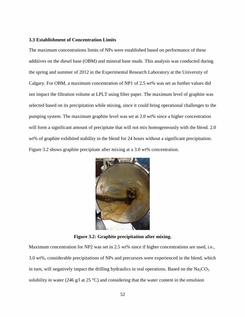
52

3.3 Establishment of Concentration Limits

The maximum concentrations limits of NPs were established based on performance of these

additives on the diesel base (OBM) and mineral base muds. This analysis was conducted during

the spring and summer of 2012 in the Experimental Research Laboratory at the University of

Calgary. For OBM, a maximum concentration of NP1 of 2.5 wt% was set as further values did

not impact the filtration volume at LPLT using filter paper. The maximum level of graphite was

selected based on its precipitation while mixing, since it could bring operational challenges to the

pumping system. The maximum graphite level was set at 2.0 wt% since a higher concentration

will form a significant amount of precipitate that will not mix homogeneously with the blend. 2.0

wt% of graphite exhibited stability in the blend for 24 hours without a significant precipitation.

Figure 3.2 shows graphite precipitate after mixing at a 3.0 wt% concentration.

Figure 3.2: Graphite precipitation after mixing.

Maximum concentration for NP2 was set in 2.5 wt% since if higher concentrations are used, i.e.,

3.0 wt%, considerable precipitations of NPs and precursors were experienced in the blend, which

in turn, will negatively impact the drilling hydraulics in real operations. Based on the Na2CO3

solubility in water (246 g/l at 25 °C) and considering that the water content in the emulsion

53

corresponds to 10%, this concentration limit was selected. Figure 3.3 shows the precipitation of

the solid precursors after mixing while preparing NP2. In addition to precursor’s precipitation,

NP2 concentrations higher than 2.5 wt% did not considerably help in filtration reduction and will

on the other hand; require higher costs and additional operational requirements. Good stability

was observed from the maximum concentration of NPs in the blends. After 4 weeks, no NPs

precipitation was observed. The same stability was reported by Zakaria (2013). The minimum

concentration of 0.5 wt% was selected based on previous research results that involved 0.2 wt%

as the minimum concentration (Nwaoji, 2012). It was concluded that concentrations >0.2 wt%

would be more representative.

Figure 3.3: NP2 precursors precipitation after mixing.

3.4 Introduction to the Experimental Analyses

LPLT and HPHT filtration tests were conducted on blends containing NP1 and NP2 using filter

papers and ceramic discs. Results were compared to the OBM control sample filtrate. The

control sample did not contain NPs and graphite. Percentage of filtration reduction was

calculated and analyzed vs. the NPs concentration. Three replicates were conducted per test.

Good repeatability was obtained. Filtration devices, details on mud mixing, and the NPs

54

preparation procedure are discussed as follow. Details on the experimental arrangements are also

addressed.

3.5 Filtration Devices

For LPLT filtration experiments, a Fann multiple unit filter press was used following the

specifications stated on the Fann LPLT Filter Press Instruction Manual 207128. Filtration

process was conducted at constant pressure of 100 psi. Filter papers with diameter of 3.5 in and

particle size retention of 2-5 microns were used in the arrangement.

HPHT testing was carried out using a 170-00-7 Ofite HPHT filter press presented in Figure 3.4.

CO2 cartridges for pressurization were used. A total differential pressure of 500 psi was applied

to the drilling fluid in the pressure cell. A pressure of 600 psi was applied from the top and a

back pressure of 100 psi was kept in the bottom. The filtration process took place at 250 °F

according to the Fann HPHT Filter Press Instruction Manual 209486. Graduated cylinders of 25

ml were used to collect the filtrate after 30 min.

Figure 3.4: 170-00-7 Ofite HPHT filter press.

55

3.6 Drilling Fluid Mixing

OBM was provided in 4-gallon containers. For NPs preparation purposes, the fluid was divided

into 1-liter vessels. A paint mixer shown in Figure 3.5 was used with a hand drill.

Figure 3.5: Paint mixer used to mix OBM.

Figure 3.6 presents the arrangement for the OBM mixing. A hole was opened on the container lid

to mix it and avoid fluid leakage. The mixing was carried out during 10 min to create a

homogeneous blend. Then, the fluid was placed in 1-liter vessels that facilitated the NPs

preparation since the NPs-containing blends were based on a 500 ml of OBM.

Figure 3.6: OBM mixing with hand drill.

3.7 Nanoparticle Preparation Procedure

A stepwise addition of solid precursors was conducted directly on the drilling fluid for in-situ

preparation of NPs. Zakaria (2013) found that that in-situ prepared NPs exhibit a higher

performance on filtration reduction in contrast to ex-situ prepared NPs. It is believed that the

56

higher water level content from ex-situ prepared NPs impairs on the NPs dispersion and

interaction with organophilic clays in the mud. The mixing procedure was carried out at high

shear rate using a Hamilton Beach 10-speed blender as shown in Figure 3.7 at 2500 rpm. 500 ml

of OBM was used as a base volume. The graphite was added following a similar method after the

NPs are formed. The maximum NPs concentration limits were selected based on an exhaustive

experimental testing that considered rheology, filter cake thickness, and precipitation while

mixing. After investigating the effect of mixing in NPs performance using different approaches,

a mixing procedure for NP1 and NP2 preparation is proposed in this work and is presented as

follows.

Figure 3.7: Hamilton Beach 10-speed blender containing drilling fluid.

3.7.1 NP1 mixing procedure

A powdered precursor called Pearl Jam (Chemfax) leads to the formation of NP1. This precursor

results from the mixing of iron hydroxide (III) and caustic soda at 90% of purity. This precursor

is sensitive to air as it quickly oxidizes. After testing different ways for the precursors addition

based on LPLT tests, the best results were obtained when NP1 at 0.5 wt% (low) were prepared

by an average addition of 2.3 g followed by 1 min of mixing at high shear rate. Concentration of

1.0 wt% (medium) is carried out by an addition of 3.5 g followed by 1 min of mixing at high

57

shear rate. Likewise, NP1 at 2.5 wt% (high) are prepared by additions of 7 g of precursors

followed by 1 min of mixing. Addition of the same amount of precursor for all the

concentrations proved to be not effective, as a significant amount of foam was obtained. This

foam is a key parameter that affects the filtration at both conditions of HPHT and LPLT.

The graphite addition was conducted similarly to the addition of the NP1 precursor. Graphite at

low concentration (0.5 wt%) was prepared by addition of 0.8 g amounts followed by 1 min of

mixing. The high graphite concentration (2.5 wt%) involved the addition of amounts of 2.35 g

followed by 1 min of mixing. An average temperature of 139°F was recorded immediately after

the blends preparation in presence of graphite. This temperature increase resulted from the

mixing at high rpm. It was observed that the longer mixing resulted in higher blend temperature.

3.7.2 NP2 mixing procedure

Soda ash (solid Na2CO3 commercial grade supplied by Canamara) and calcium chloride (solid

CaCl2 commercial grade supplied by Canamara) at 90% of purity are the basic precursors for the

preparation of the NP2. Soda ash is first added to the fluid using a stepwise addition similar to

that described for NP1. Then, the calcium chloride is added similarly. The optimum procedure

for addition of precursors was determined through testing under LPLT while controlling the

amount of foam formed. Low concentration of NP2 requires the addition of 0.93 g for each

precursor followed by 1 min of mixing. Medium concentration of NP2 is prepared following the

same procedure for the preparation at low concentration. The high concentration follows

additions of 1.8 g of precursors followed by 45 s of mixing. Low and high addition of graphite is

conducted similarly to the procedure used for NP1. An average temperature of the blend of

131°F was recorded after the NP2 preparation in presence of graphite. A similar value was

reported for NP1 and this gives an idea of the temperature range at which the NPs are stable.

58

3.7.3 Rheology analysis

The rheological properties of the blends were measured at a standard test temperature of 120°F

(API Recommended Practice 13D). These included plastic viscosity (PV), yield point (YP), gel

strength at 10 sec (10 s GS) and 10 min (10 min GS). Measurements were performed at two

graphite levels: low and high. Most of these parameters fell within acceptable ranges, whereas

the yield point deviated a little at some combination of concentrations. Table 3-4 presents the

test matrices, which illustrates the nomenclature used to report the rheology results.

Concentrations are expressed in wt %. Rheology results are presented in Table 3-5.

Table 3-4: Tests matrices for rheology testing of NP1 and NP2.

NP1

0.5% 1.0% 2.5%

Graphite

0.5% DF1 DF2 DF3

2.0% DF4 DF5 DF6

NP2

0.5% 1.0% 2.5%

Graphite

0.5% DC1 DC2 DC3

2.0% DC4 DC5 DC6

The nomenclature “DF” is used to indicate that the blend is composed of OBM with presence of

iron-based NPs (NP1). The expression “DC” stands for a blend composed of OBM and calcium-

based NPs (NP2). The numbering is performed to differentiate between different concentrations;

including that of graphite. NP2 blends give an average increase in gel strength of around two

units in comparison to the control sample at 10 s and 10 min. Increase of about 2 units in average

on the value of plastic viscosity was experienced by NP2 blends. NP1 causes reduction in the

yield point of the blends especially at high graphite concentration. The addition of graphite did

not significantly impact the plastic viscosity and gel strength of the blends containing NP1.

59

However, this is not the case for blends containing NP2, where the addition of graphite led to an

increase of PV on around 4 units in comparison to the blends with low graphite content. High

level of graphite was also observed to have an effect on gel strength in NP2 blends.

Table 3-5: Rheology results for all blends (DF stands for iron-based blends and DC1 stands

for calcium-based blends).

Composition

Rheology @ 120°F

PV

(cP)

YP

(lb/ft2)

Gel 10 s

(lb/100ft2)

Gel 10 min

(lb/100ft2)

DF1 13 3.0 2.0 2.3

DF2 13 0.0 2.0 2.2

DF3 13 1.0 2.0 2.3

DF4 12 0.0 1.8 2.4

DF5 13 0.0 2.0 2.2

DF6 13 0.0 1.8 2.2

DC1 15 3.0 3.5 4.0

DC2 14 5.0 3.0 3.5

DC3 14.5 2.0 3.8 4.0

DC4 18 5.0 4.2 4.6

DC5 19 6.0 4.5 5.2

DC6 21 5.0 4.8 5.9

In general the rheology was not significantly affected by the addition of NPs due to the small

concentrations. Zakaria (2013) also reported a slight change in rheology parameters due to NPs

addition on OBM. Slight reduction on PV by addition of NP1 are due to the presence of the

hydroxyl group (OH-) on the NPs surface that creates agglomeration and a higher mass of

selective physisorption of organic clay suspension on the NPs free surface (Srivasta, 2010).

Reduction of blends rheology by addition of NP1 was also a finding in Zakaria (2013) research

work. The reduction on the yield point by addition of NP1 is believed to occur due to the anionic

60

nature of hydroxyl group and their interaction (acting as a thinner) with the charged edges of the

suspended clays on the mud. This effect can be seen as an analogy of the work performed by

deflocculants (commonly anionic polymers) that neutralize positive charges on clay surfaces and

prevent flocculation (SLB Oil Field Glossary). A polymeric fatty acid having concentrations of

0.5-3.0 lb/bbl (1.4-9.0 kg/m3) or organophilic clay at concentrations of 1-6 lb/bbl (3-17 kg/m

3)

can be used in NP1 to improve the rheological and suspension properties (Baroid Drilling Fluid

Manual, 1997). Note that the organophilic clay requires a polar additive such as water to develop

a higher yield point which may impact the NPs performance.

Addition of NP2 increased the plastic viscosity of the blends. The viscosity increase by addition

of calcium-based NPs has also been reported by Zakaria (2013). Manea et al. (2012) reported

increase in viscosity of the blends by addition of calcium carbonate microparticles. The NP2

bridging capability on invert emulsions is believed to be the reason for the plastic viscosity

increase and rheological stability Zakaria (2013).

3.8 LPLT Filtration Analysis

Percentage of filtrate reduction under LPLT after 30 min for different NPs concentrations and

graphite as LCM are presented in Figure 3.8. The percentages were calculated based on a

filtration of 7.0 ml at 30 min for the control sample. Three replicates were conducted per

experiment and the standard deviation is shown in the figure for each point. Also, the effect of

the NPs on the filtration was quantified by testing blends only containing graphite, i.e., 0 wt% of

NPs. At higher concentrations of NP1, a higher filtrate reduction is obtained for the two levels of

graphite. At 0 wt% NP1, the graphite level gave a filtrate reduction difference >10%. However,

61

at concentrations larger than 1 wt% of NP1 the graphite level did not play a crucial role in the

filtration reduction trends.

(a) (b)

Figure 3.8: (a) Percentage of reduction in mud filtration at 30 min under LPLT for NP1.

(b) Percentage of reduction in mud filtration at 30 min under LPLT for NP2.

After the filtration experiments, the filter cake thickness was characterized to allow a

comprehensive results analysis. Figure 3.9 presents photographs of filter cakes collected

following LPLT measurements. Cake thickness is quoted as one important characteristic of the

filter cakes. Just a slight increase in thickness was experienced by the addition of the graphite.

Figure 3.10 presents photos of filter cakes collected following LPLT tests in the presence and

absence of NP1 and NP2. For NP1, note that in comparison to the control sample (sample with

no NPs and graphite), blends containing low graphite level (DF1, DF2, and DF3) just give an

average 25.3% of thickness increase. Blends containing high graphite concentration (DF4, DF5,

and DF6) yield 4.7% of thickness increase in comparison to the blends containing low graphite

and 31.3% with respect to the control sample.

62

Figure 3.9: Filter cake characterization for control sample and blends containing graphite

at low and high concentrations at LPLT.

NP2 blends containing low graphite level yield a 33% thickness increase in comparison to the

control sample. Likewise, blends containing high graphite concentration gave a 35% thickness

increase. Just a 1.5% thickness increase was the result of going from low to high graphite

concentration. Filter cake characterization concluded that both types of NPs are effective

additives for filtration reduction in OBM, only creating a slight increase in filter cake thickness

which will prevent the occurrence of stuck pipe.

Figure 3.11 shows a plot that simultaneously shows % of filter cake thickness increase (right

vertical axis) and % filtrate reduction (left vertical axis). These parameters are plotted vs. NPs

concentration. The points are based on average filtration reductions and filter cake thicknesses.

High NPs concentration and high level of graphite (red line) yields thicker cakes, however, the

level of graphite is barely affecting the filtration trends.

Sample Description and Thickness Filter Cake after 30min

0.6±0.2mm

0.5±0.1mm

0.65±0.2mm

Control Sample (CS)

Graphite 0.5wt%

Graphite 2.0wt%

63

(a) (b)

Figure 3.10: (a) Filter cake characterization for control blends containing NP1 at LPLT.

(b) Filter cake characterization for control blends containing NP2 at LPLT.

It can be inferred that NP1 concentration of 1 wt% is the best performing since further addition

of NPs will not have a strong impact on the performance. At LPLT, addition of NP1 up to 2.5

wt% helps in forming an effective seal until reaching 100% of filtration reduction. This may be

due to the good interaction between NP1 nanoparticles and the organophilic clays contained in

the mud. NP1 are believed to have a good interaction with the negative edges of the clays

(Zakaria, 2013). It was observed that at higher concentration of NP2, a slightly less reduction in

the filtrate is obtained. Nonetheless, the positive effect of the NPs is evident when comparing the


0.63±0.2mm

0.65±0.1mm

0.66±0.1mm

0.66±0.2mm

0.62±0.3mm

DF4

DF5

DF6

DF2

DF1

DF3

0.63±0.1mm

0.68±0.2mm


0.66±0.1mm

0.67±0.1mm

DC2

DC3

DC4

DC5

DC6

0.67±0.1mm

0.67±0.2mm

0.68±0.2mm

DC1

64

results to the case at 0 wt% NPs. From the previous figure it can be concluded that as NPs

concentration increases, the effect of graphite level becomes less important particularly for NP1.

(a) (b)

Figure 3.11: % filtrate reduction (left axis) compared to % filter cake thickness increase

(right axis) for (a) NP1 and (b) NP2.

NP2 performance as a filtration reduction agent indicates that a concentrations >0.5 wt%, further

improvement in filtrate reduction is not obtained. This may happen due to an increase in NPs

aggregation and this fact can be supported by analyzing the filter cake thickness increase

obtained. In general it was observed that NP1 is superior in performance in comparison with

NP2. NP2 concentration of 0.5 wt% is the best performing since further addition of NPs did not

impact the filtration reduction significantly, and in turn, will carry additional operational issues

(eventual precipitation) and higher expenses. Overall, the performance of NP1 blends is better

compared to NP2 blends at LPLT.

The individual effect of graphite addition to the blends was evaluated at the optimum

concentrations (1.0 wt% for NP1 and 0.5 wt% for NP2) in an earlier research stage. Only NP1 at

1.0 wt% gives 90% filtration reduction. NP2 at 0.5 wt% gives 31.3% of filtrate reduction. By

65

looking at Figure 3.11 at these mentioned concentrations, it is concluded that graphite addition

yields a slight improvement in filtration reduction at LPLT in combination with NPs. This could

be explained by considering that the graphite will help in the creation of a more effective seal

due to its wider range of particle sizes.

3.9 HPHT Filtration Analysis

2.5” x 0.25” ceramic discs that simulate a porous media of 775 md (mean pore throat of 10

microns) were utilized under HPHT conditions to evaluate the effect of NPs in the reduction mud

filtrate. These ceramic discs are the ones with the lowest commercially available permeability.

The lowest permeability was selected to resemble the permeability of sandstone samples in later

wellbore strengthening tests. The pressurization was conducted using CO2 cartridges. A back

pressure of 100 psi was used. Figure 3.12 summarizes the percentage of filtrate reduction when

NPs were used relative to 6.0 ml at 30 min obtained for the control sample. Three replicates were

conducted per experiment and the standard deviation is shown. Filtration reduction trends can be

visualized. NP1 concentration of 0.5 wt% and NP2 concentration of 2.5 wt% gave the best

performance. In order to conduct an insightful interpretation of the results, the filter cake

thickness after 30 min for each experiment was characterized. Figure 3.13 presents the filter cake

characterization for the control sample (sample without presence of NPs and graphite), blends

containing only graphite at low and high concentrations and blends containing only NPs at the

best performing concentrations mentioned previously. Just a slight increase in thickness was

observed by the addition of only graphite and NPs to the blend.

66

(a) (b)

Figure 3.12: (a) Percentage of reduction in mud filtration at 30 min under HPHT for NP1.

(b) Percentage of reduction in mud filtration at 30 min under HPHT for NP2. 775 md

ceramic discs were used in the filtration experiments.

Figure 3.13: Filter cake characterization for CS and blends containing graphite at low and

high concentrations and blends containing just NP1 and NP2 respectively at HPHT.


1.5±0.1mm

1.6±0.1mm

1.71±0.3mm

Graphite 0.5wt%

Graphite 2.0wt%

Control Sample (CS)

Only 0.5 wt% NP1

Only 2.5 wt% NP2

1.6±0.5mm

1.5±0.3mm

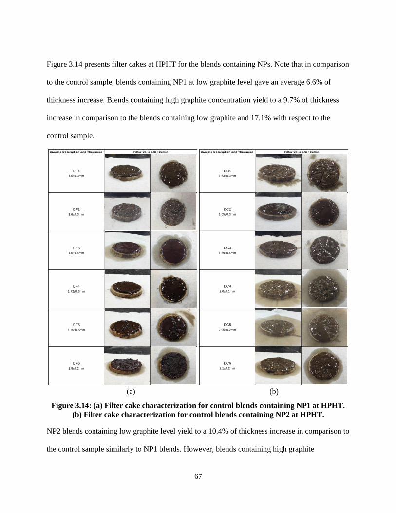
67

Figure 3.14 presents filter cakes at HPHT for the blends containing NPs. Note that in comparison

to the control sample, blends containing NP1 at low graphite level gave an average 6.6% of

thickness increase. Blends containing high graphite concentration yield to a 9.7% of thickness

increase in comparison to the blends containing low graphite and 17.1% with respect to the

control sample.

(a) (b)

Figure 3.14: (a) Filter cake characterization for control blends containing NP1 at HPHT.

(b) Filter cake characterization for control blends containing NP2 at HPHT.

NP2 blends containing low graphite level yield to a 10.4% of thickness increase in comparison to

the control sample similarly to NP1 blends. However, blends containing high graphite


1.6±0.3mm

1.6±0.3mm

1.6±0.4mm

1.72±0.3mm

1.75±0.5mm

1.8±0.2mm

DF3

DF4

DF5

DF6

DF2

DF1

2.1±0.2mm


1.63±0.3mm

1.65±0.3mm

1.69±0.4mm

2.0±0.1mm

2.05±0.2mm

DC5

DC6

DC2

DC3

DC4

DC1

68

concentration gave a 36.6% of thickness increase. 23.7% of thickness increase is obtained by

increasing graphite concentration from low to high. Compared to what happened in NP1 blends

at high graphite concentration, NP2 blends at high graphite concentration give a significantly

thick filter cake. Figure 3.15 compares in the same plot filtration reduction and filter cake

thickness for each NP type to facilitate the results interpretation. Filter cake thickness increase is

referred to the right vertical axis and % HPHT filtrate reduction is referred to the left vertical

axis. These parameters are plotted vs. NPs concentration. Curves were constructed based on

average filtration reductions and filter cake thicknesses. At low graphite concentration there is no

significant effect of NP1 and NP2 addition on filter cake thickness. At high graphite

concentration, there is an increase on the cake thickness as NP1 and NP2 concentrations become

higher.

(a) (b)

Figure 3.15: % HPHT filtrate reduction (left axis) compared to % filter cake thickness

increase (right axis) for (a) NP1 and (b) NP2.

Contrary to what happened at LPLT conditions, the best filtrate reduction was obtained at the

lowest NP1 concentration. This is due to the stability of NP1 at HPHT conditions.

69

High concentration of NP1 at HPHT may result in poor interaction between the NPs and the

clays creating significant NPs agglomeration and a high-permeability cake. This claim is

corroborated by analyzing the filter cake thicknesses increase. For field application purposes this

is a useful finding since it is always advisable to work under low-additives concentration for

economic and environmental reasons. The increase of filtrate reduction with respect to the blend

containing 0 wt% of NPs was significant and this corroborates the success of the NP1 in

reducing filtration. The graphite addition up to a high level of 2.0 wt% demonstrated beneficial

results for filtrate reduction especially at NP1 concentrations less than 2.5 wt%. The graphite

effect is not that significant at high NP1 concentrations. At HPHT conditions, NP2 work better

at high concentration in contrast to what was observed at LPLT, where higher filtrate reductions

were obtained at low concentrations. It is believed that at HPHT, NP2 exhibit a good dispersion

into the mud (Zakaria, 2013). NP2 proved to have an effect on filtrate reduction in comparison to

the case in which 0 wt% of NPs was tested. For NP2, increasing the graphite concentration to

2.0 wt% resulted in a negative effect in filtration. This is due to the interaction between NP2 and

graphite at HPHT, which is evident from the significant increase in the filter cake thickness. This

high thickness indicates the poor agglomeration of the NPs and graphite during the filtration

process and therefore the performance at low graphite concentration is better when using this

type of NPs. Similar to the LPLT testing, as the NPs concentration is increased, the effect of the

graphite concentration becomes less pronounced for filtration reduction particularly for NP1.

NP2 at 2.5 wt% was observed to be the best performing concentration since it gave higher

filtration reduction. Overall, the performance of NP1 blends is better compared to NP2 blends at

HPHT. It was observed that thicker cakes imply a less efficient filtration reduction process.

70

Investigation of the individual effect of the NPs and graphite on filtration reduction was carried

out at the best performing concentration for each NPs type. A blend containing NP1 at 0.5 wt%,

with no graphite was tested at HPHT on a ceramic disc and the result is plotted as a green dot in

Figure 3.16 giving a 50% of filtrate reduction.

Figure 3.16: Percentage of reduction in mud filtration at 30min under HPHT for NP1. The

green dot represents the blend only containing NP1 at 0.5 wt%.

Figure 3.16 shows that 0.5 wt% of NP1 gives a higher filtrate reduction than pure graphite at

both 0.5 wt% and 2.0 wt%. This confirms the superior performance of the NP1 in comparison to

a conventional LCM. The blend consisting of 0.5 wt% of NP1 and 0.5 wt% of graphite is slightly

improving the performance in comparison to the use of just NP1. However, the situation in

which 0.5 wt% NP1 is combined with 2.0 wt% graphite, gives a more pronounced improvement.

Likewise, a blend containing 2.5 wt% of NP2 was tested at HPHT resulting in the green dot on

Figure 3.17 with a 30.9% of filtrate reduction. NP2 at 2.5 wt% gives a higher filtrate reduction

than just graphite at both 0.5 wt% and 2.0wt%. Similarly to the situation with NP1, NP2

performed better than just conventional LCM. By combining 2.5 wt% of NP2 and 2.0 wt% of

graphite, just a slight increase in filtrate reduction is observed. This could be due to

agglomeration between NP2 and graphite both at the highest level; this condition in fact yields to

71

the highest filter cake thickness. When a combination of 2.0 wt% of NP2 and 0.5 wt% of graph

is conducted, a higher filtrate reduction is obtained in comparison to the system containing just

NP2 at 2.5 wt%. This means that at high level of NP2, just a small amount of graphite is needed

to create an effective seal. Results from filtration experiments show that at this concentration, the

best performance in filtration reduction was achieved.

Figure 3.17: Percentage of reduction in mud filtration at 30 min under HPHT for NP2. The

green dot represents the blend only containing NP2 at 2.5 wt%.

The mud cake characterization in a porous media shed a light on the utilization of these NPs

types during drilling operations using OBM. Figure 3.18 shows a cross-section of a ceramic disc

after testing of blend DF3. Note that the fluid invasion cannot be easily observed just by looking

at the ceramic disc cross-section.

Figure 3.18: Cross-section of ceramic disc after DF3 blend testing at HPHT.

16.7% 23.3% 30.9%

72

A SEM analysis to characterize the NPs size on filter cakes was conducted by Zakaria (2013) as

part of his doctoral thesis for the Drilling Research Team at the University of Calgary. WBM

was used in the analysis due to the complexity of SEM images on OBM systems. NP1 were able

to create a smooth surface on the filter cake that proves their ability to accommodate into the

small spaces created by larger particles. Figure 3.19 shows a plot of a SEM image without and

with NP1. From Figure 3.19 (b) it is possible to visualize that NP1 creates a smooth surface free

of cracks. Figure 3.19 (a) shows a rough surface, with significant cracks in absence of NP1. This

corroborates the ability that NP1 have on reducing the filtrate at HPHT and LPLT since flow is

believed to be uncontrolled through cracks and cakes imperfections.

Figure 3.19: SEM image of filter cake for blend (a) without NP1 and (b) with NP1

(Zakaria, 2013).

NP2 were also analyzed using SEM images in presence of WBM. In comparison to NP1effect on

filter cake, addition of NP2 nanoparticles did not give smooth cake surfaces as evidenced by

Figure 3.20 that shows a SEM image of a filter cake with and without NP2. This helps to explain

the superior performance of NP1 over NP2 in terms of filtration reduction. Results obtained from

SEM analysis agree with the findings reported in this chapter.

73

Figure 3.20: SEM image of filter cake for blend (a) without NP2 and (b) with NP2

(modified from Zakaria, 2013).

3.10 Summary

The experimental research conducted in this chapter proved the successful application of in-

house prepared NPs and LCM in reducing mud filtration in a porous media using OBM.

Filtration performance vs. NPs concentration was investigated and results will serve as the first

wellbore strengthening performance indicators. Blends (composed by a specific NP type) that

provided the best performance on filtration reduction are expected to have a better effect in

wellbore strengthening. These findings are anticipated to be of significant impact in drilling

operations to mitigate the formation damage due to fluid invasion. The most remarkable findings

from this analysis are:

- NP1 and NP2 reduced mud filtration on a porous media simulated by ceramic discs under

HPHT conditions with filtrate reductions up to 76% with NP1. NP1 blends yield to the higher

filtration reduction at LPLT and HPHT

- NP1 and NP2 worked successfully at LPLT. NP1 reached up to 100% filtrate reduction. Better

results are obtained at higher graphite concentration at these conditions

74

- Acceptable filter cake thicknesses (< 40% increase compared to control sample) were obtained

for both LPLT and HPHT conditions. The graphite level has a significant effect on filter cake

thickness at HPHT compared to LPLT conditions particularly for NP2-blends. Excessive mud

thicknesses were associated with non-effective filtration processes. NPs agglomeration may

result in high-permeability and thicker cakes

- Blends that combined NPs and graphite gave superior performance compared to blends

containing graphite in absence of NPs

- NP1 worked better at lower NPs concentrations at HPHT. NP2 gave better filtrate reduction at

higher NPs concentrations at HPHT. At LPLT, NP2 performed reasonably better at low NPs

concentrations

- In blends containing NP2 at HPHT, low graphite level worked more efficiently due to the thick

cakes formed at high graphite concentration. Poor interaction between NPs and clays on blends

is believed to be the reason

- Rheology of the blends is not significantly affected by the addition of NPs and LCM. This

allows the consideration of these blends for practical field applications in the presence of some

viscosifiers/suspending agents

75

Nanoparticles Application for Wellbore Strengthening in Sandstone Cores Chapter Four:

4.1 Introduction to the Experimental Analysis

Wellbore strengthening in sandstone cores was evaluated using NPs and graphite as LCM with

OBM. Sandstone cores with a wellbore that is cased and cemented were used to scale a well into

laboratory dimensions. This core was then placed into a hydraulic fracturing apparatus which

applies overburden and confining pressure and allows injection of fluid into the wellbore using

syringe pumps. More than one injection cycle was carried out and software constructed on

LabVIEW® platform tracked all the injection parameters vs. time.

This research involved tensile strength, porosity, and permeability characterization. The sample

preparation was part of the work carried out by the author and included a long and exhaustive

process that started with drilling of the cores from sandstone slabs, drilling of the wellbore,

setting of casings and steel caps and finally grinding of the cores to obtain a smooth surface that

allows application of confining pressure evenly. After the core was tested, cleaning of the steel

caps was required for use in future tests. Wellbore strengthening was obtained using NPs in

OBM and trends as a function of NPs and graphite concentration were identified. Impact of

HPHT filtration was quantified on wellbore strengthening and the match between these two

parameters was investigated. The wellbore strengthening mechanism was identified based on

experimental evidence from optical microscopy, SEM, and EDX analysis. These original

findings give insights for field applications and operational design. The sandstone cores

preparation and testing was carried out during the winter, spring and summer of 2013 by the

author at the Missouri University of Science and Technology with strong support received from

faculty and staff of this institution.

76

4.2 Experimental Facilities and Apparatus

This research was carried out in a cooperative agreement between the University of Calgary and

the Geologic Sciences and Engineering Department at the Missouri University of Science and

Technology. The wellbore strengthening and filtration experiments were conducted in the

Drilling Fluids Laboratory. This is a fully equipped facility used for graduate research and also

for undergraduate student’s drilling fluids laboratory sessions. The sandstone cores preparation

was carried out by the author at the Missouri S&T Rock Mechanics and Explosive Research

Center (RMERC). Rock surface grinding, drilling arrangements, and steel caps cleaning were

performed mainly in the RMERC workshop. Part of this work was also conducted at the McNutt

Hall drilling fluids laboratory.

The rock drill shown in Figure 4.1 was used for drilling sandstone cores of different diameters

for hydraulic fracturing experiments, Brazilian tests to determine tensile strength, and for

porosity and permeability measurements. Diamond insert core bits of diameter 53/4

”, 2” and 1”

were used respectively. Water was injected through the annular and ended up into a water pool

that is located below the drilling table. The drilling operation had to be conducted very slowly in

order to get a smooth core surface. An average rate of penetration of 1 in/15 sec was used.

Figure 4.2 shows the saws used for cuttings slides from sandstone cores for removing of rock

imperfections as natural fractures and also for the cutting of discs for microscopy and SEM

analysis. The big saw uses water as a lubricant that goes through the annular. The small samples

saw cuts dry and even surfaces can be obtained in a short period of time.

77

Figure 4.1: Rock drill.

Sandstone cores for Brazilian tests and porosity and permability testing were grinded using the

grinder shown in Figure 4.3 to get smooth surfaces.

(a) (b)

Figure 4.2: (a) Rock Saw. (b) Small samples saw.

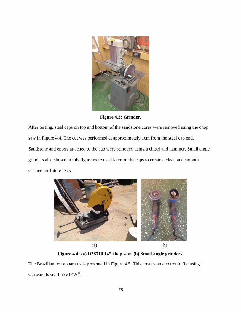
78

Figure 4.3: Grinder.

After testing, steel caps on top and bottom of the sandstone cores were removed using the chop

saw in Figure 4.4. The cut was performed at approximately 1cm from the steel cap end.

Sandstone and epoxy attached to the cap were removed using a chisel and hammer. Small angle

grinders also shown in this figure were used later on the caps to create a clean and smooth

surface for future tests.

(a) (b)

Figure 4.4: (a) D28710 14” chop saw. (b) Small angle grinders.

The Brazilian test apparatus is presented in Figure 4.5. This creates an electronic file using

software based LabVIEW®.

79

Figure 4.5: Brazilian test apparatus.

The hydraulic fracturing tests are conducted using a hydraulic fracturing apparatus that was

designed and assembled at the Missouri University of Science and Technology. This apparatus is

presented in Figure 4.6 and is located at the Drilling Fluids Laboratory. The operating schematic

of this apparatus is presented in detail in Figure 4.7. This apparatus has served for previous

research projects (Liberman, 2012; Nwaoji, 2012) where wellbore strengthening was

investigated using WBM, OBM and several types of rocks. However, shale cores were not tested

before. Cores of different length were also tested.

The pump system is composed of a 10,000 psi/100 ml Isco DX100 syringe pumps shown in

Figure 4.8. This pump applies the confining pressure and injects fluid into the wellbore. Water is

the working fluid in these pumps. The water is placed in stainless steel containers that are refilled

from a water reservoir. An inlet valve allows fluid flow into the pump during refilling and

discharge. Stainless steel lines of 1/8” and 1/4” OD allows distribution to and from the pumps

and to the hydraulic fracturing apparatus. Outlet valves in each pump prevent depressurization of

the system while being refilled.

80

Figure 4.6: Hydrualic fracturing apparatus.

Figure 4.9 presents the mud accumulator system. A stainless steel pipe with an internal piston is

in charge of the accumulation and injection of fluid into the pressure cell. The accumulator is

loaded with drilling fluid that comes from an upper plastic container. This fluid is placed into the

accumulator at 60 psi. The water injection from the pump takes place from the lower part of the

piston and this causes the drilling fluid to go to the core sample line. It is important to clean the

mud accumulator if OBM is planned to be used as the system was previously used to pump

WBM or vice versa. In this research, a careful cleaning of the mud accumulator was performed

by removing the caps and piston using a vise in the workshop. Detergent was used to remove

WBM that remained. O-rings and gaskets were also cleaned and the accumulator was re-

assembled in the hydraulic fracturing arrangement.

81

Figure 4.7: Schematic of hydraulic fracturing apparatus (Liberman, 2012).

82

Figure 4.8: Isco DX100 syringe type pumps (Liberman, 2012).

The hydraulic pump provides the overburden load to the sample. This pump is connected to a

piston located on top of the arrangement. This piston is illustrated in Figure 4.10. Axial load is

applied to the steel caps over the sample by the piston which creates the overburden load.

Figure 4.9: Mud accumulator system (Liberman, 2012).

83

Figure 4.10: Overburden piston (Liberman, 2012).

A rubber sleeve is used to apply confining pressure to the sample. This rubber sleeve is presented

in Figure 4.11. Water coming from the syringe pumps is used to fill the sleeve and apply the

confining pressure.

Figure 4.11: Rubber sleeve top view.

The data acquisition software is based on a LabVIEW® platform and was provided by the pump

manufacturer. The purpose of this software is to record pressure vs. time during fluid injection

into the core. The pump controller is connected to an rs-232 serial port on the computer. This

system is also designed to measure pressure losses in the system.

84

4.3 Sandstone Cores Characterization

4.3.1 Composition

The Roubidoux sandstone used in these experiments was obtained from outcrops located in

Jefferson City (mid-Missouri). This type of rock is an Ordovician, medium grained, laminated to

thinly bedded quartz sandstone. XRD analysis showed a composition of 94% of quartz and 6%

of kaolinite (Abu Bakar and Gertsch, 2011).

Three Roubidoux slabs of 12”(l)x12”(w)x9”(t) were provided. Two slabs are presented in Figure

4.12.

Figure 4.12: Roubidoux sandstone slabs.

4.3.2 Porosity and permeability

The Roubidoux sandstone porosity was measured experimentally using mercury injection. Figure

4.13 shows the small cores (1” x 2”) used in the measurement. Each core was drilled from a

different rock slab.

Figure 4.13: 2”x 1” Sandstone cores for porosity and permeability measurements.

85

Table 4-1summarizes the porosity results. The grain density was also determined for each core.

An average porosity value of 0.14±0.01 in fraction was obtained.

Table 4-1: Sandstone porosity results.

Slab Sample d (mm) L(mm) A (cm2) V (cm

3) Mass (g) Density (g/cm

3) Porosity

1 25.09 52.27 4.94 25.84 58.64 2.27 0.14

2 25.04 52.02 4.92 25.62 57.63 2.25 0.15

3 25.07 51.30 4.94 25.32 57.08 2.25 0.15

The absolute permeability tests were conducted by using nitrogen injection. The results are

presented in Table 4-2. An average value of 12.7 ±3.1 md is calculated for the three samples.

Table 4-2: Sandstone permeability results.

Slab Sample Permeability (md)

1 10.5

2 16.2

3 11.4

4.3.3 Tensile strength

The tensile strength was determined by the Brazilian test arrangement presented in Figure 4.5.

Rock samples of 2” x 1” were used. These samples were obtained from three sandstone rock

slabs by drilling with a 2” diamond core insert bit. Then, the samples were cut using the rock saw

from Figure 4.2(b) every 1”. Three replicates were conducted per rock slab. Figure 4.14 presents

the samples after testing. Samples from slabs 1, 2, and 3 are labeled as (a), (b), and (c).

Table 4-3 shows the results for the three replicates conducted per rock slab. The Roubidoux

sandstone UCS is quantified in 12325 psi (Salehi and Nygaard, 2012).

Based on the porosity, permeability, and tensile strength values it can be concluded that the three

rock slabs used for the sample can be considered as the same porous media.

86

(a) (b) (c)

Figure 4.14: Sandstone cores after Brazilian test for (a) Slab 1, (b) Slab 2, and (c) Slab 3.

Table 4-3: Tensile strength for the three sandstone slabs.

Slab Sample Tensile Strength (MPa)

1 2.40 ± 0.46

2 2.24 ± 0.13

3 2.33 ± 0.10

4.4 Sandstone Cores Preparation

The sandstone core preparation consists of the next main steps:

Drilling of 53/4

” cores from slabs

Drilling of 9/16” wellbore in the center of the cores

Casing assembly on steel caps and cementing of caps in cores

Cement dry out

Core surface grinding

Core vacuuming and saturation

Post-testing caps cleaning

87

These core preparation steps take a minimum of four days per core. Each step needs to be

conducted carefully to ensure repeatability of the same initial parameters for each test. A

description of each of the core preparation steps is presented as follows.

4.4.1 Drilling of 53/4

” cores from slabs

The core preparation starts with drilling of 53/4

x 9” cores from the rock slabs. A 53/4

” diamond

insert core bit was used as shown in Figure 4.15. The core slab is secured in the drill table using

a chain. The drilling operation of the core is also illustrated while water is injected to lubricate

the bit and for cuttings removal. The slab needs to be well secured otherwise vibration is

experienced and the core surface obtained is not smooth. A smooth surface is required on the

cores to be able to apply confining pressure evenly.

(a) (b)

Figure 4.15: (a) Sandstone core drilling arrangement. (b) Sandstone core drilling while

pumping water.

Figure 4.16 shows a top view of the slab after the drilling of the first core and five drilled cores

obtained from rock slabs.

88

(a) (b)

Figure 4.16: (a) Rock slab after drilling the first core. (b) Sandstone cores.

4.4.2 Drilling of 9/16” wellbore in the center of the cores

9/16” wellbores were drilled in the center of the cores. This was done to recreate a real well into

a sandstone formation. The first approach consisted in the design of a guide built from a wood

circle surrounded with a metal plate as shown in Figure 4.17. The core is secured using a chain at

tension. Due to significant vibration created by this arrangement the wellbore obtained was not

exactly vertical. This presented a challenge since steel caps and attached casings require a

wellbore exactly in the center of the core since a smooth surface is necessary between the core

and the cap.

Figure 4.17: Wellbore drilling on sandstone core.

89

Due to this situation a different approach was taken. A guide built from a PVC pipe along with a

wood circle at the top of the cap was constructed and secured with screws. The slab where the

cores where taken from served as the guide to avoid vibration. The core and the guide are placed

together into the hole in the core slab as shown in Figure 4.18. With this approach the vibration

was mitigated and straight wellbores were obtained. Also illustrated is a core after the wellbore

drilling once the guide is removed. The core then needs to be removed carefully by raising the

end of the slab and removing it from the bottom. At least two people are required to conduct the

core removal.

(a) (b)

Figure 4.18: (a) Wellbore drilling on sandstone core using a PVC guide. (b) Sandstone core

after wellbore drilling.

4.4.3 Casing assembly on steel caps and caps cementing on cores

9/16” OD steel casings are assembled in steel caps. Teflon is used in the casing threads and a

vise is used in this assembly. Steel caps and casings are presented in Figure 4.19. These caps are

cemented at the top and bottom core ends.

90

Figure 4.19: Steel caps for top and bottom ends of cores.

High-strength structural epoxy paste is used as the cementing medium of the steel caps on the

core ends. Figure 4.20 shows the epoxy used. A mix ratio of 1:1 is required for the epoxy

preparation. Epoxy mixing procedure is also illustrated. This should be performed for at least 2

min.

(a) (b)

Figure 4.20: (a) Epoxy. (b) Epoxy after mixing.

A thin layer of epoxy is placed on the caps surface and also on the core end. Epoxy is also placed

on the casing walls to ensure casing attachment to the wellbore. The cap is then placed over the

core and three clamps with an angle of 120° between them are used to exert pressure and ensure

well-attachment as illustrated in Figure 4.21.

91

4.4.4 Cement dry out

For each cemented cap, a total of 24 hours is required for cement dry out. After 24 hours of

placing the first cap, exactly the same procedure is carried out for the second one. This means a

total of 48 hours per core. The arrangement, as ilustrated in Figure 4.21, is then conducted. Note

that the core on the left of Figure 4.21 has only one cap cemented while the core on the right has

two cemented caps.

Figure 4.21: Sandstone cores and steel caps cementing dry out using clamps.

4.4.5 Core surface grinder

After the steel caps are cemented at the top and bottom of the core, cement excess needs to be

removed to create a smooth surface between the core and the steel cap. A hand grinder shown in

Figure 4.22 was used for this purpose. The bottom line of the grinding procedure is to create a

smooth surface free of gaps along the core. The grinding needs to be conducted carefully in order

to mitigate all the irregularities in the core surface that can potentially damage the confining

sleeve.

92

Figure 4.22: Hand grinder for core surface.

4.4.6 Core vacuuming and saturation

The core was vacuumed for 24 hours using the vacuum chamber in Figure 4.23. This vacuum

chamber was connected to a vacuum pump using the yellow line.

Figure 4.23: Sandstone core vacuuming arrangement.

The soaking of the core was carried out with the vacuuming pumping still on. Water was added

to the chamber by immersing the water inlet pipe into a container filled with water. The valve is

93

then opened to allow the flow of water into the chamber. Once the core is completely immersed

the valve is closed. The core was saturated for 8 hours with the vacuum pump on.

4.4.7 Post-testing caps cleaning

After the hydraulic fracturing testing, the steel caps were removed and cleaned for the next stage

of the experiments. Steel caps removal is performed with the set-up presented in Figure 4.24

using a chop saw. Once the caps are removed from the core, surface grinding was performed to

remove rock and cement. This was conducted using a small angle grinder as shown in Figure

4.25. This needs to be done carefully to create a smooth surface free of epoxy for the next

cementing procedure.

Figure 4.24: Steel caps removing.

4.5 Challenges Faced and Solutions in Sandstone Cores Preparation

The main challenges faced on the sandstone core preparations were:

Drilling a straight wellbore in the center of cores

Removal of a natural fracture from cores

A description of the challenges and solutions are presented as follows.

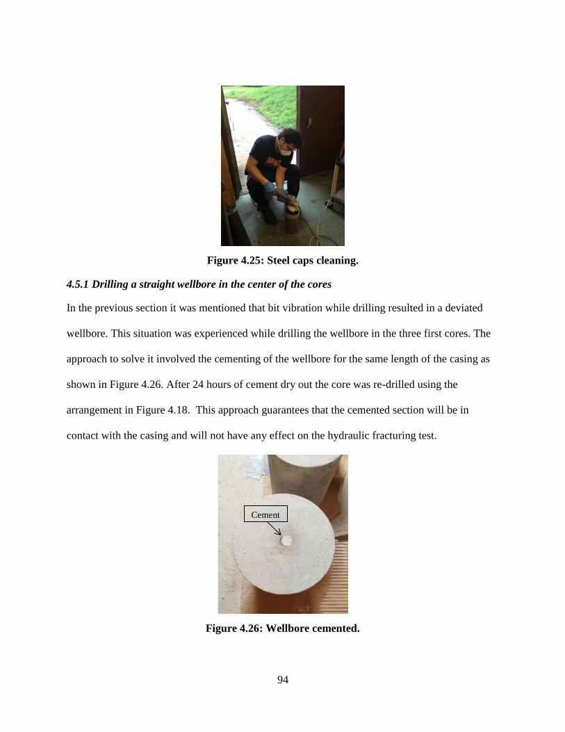
94

Figure 4.25: Steel caps cleaning.

4.5.1 Drilling a straight wellbore in the center of the cores

In the previous section it was mentioned that bit vibration while drilling resulted in a deviated

wellbore. This situation was experienced while drilling the wellbore in the three first cores. The

approach to solve it involved the cementing of the wellbore for the same length of the casing as

shown in Figure 4.26. After 24 hours of cement dry out the core was re-drilled using the

arrangement in Figure 4.18. This approach guarantees that the cemented section will be in

contact with the casing and will not have any effect on the hydraulic fracturing test.

Figure 4.26: Wellbore cemented.

Cement

95

4.5.2 Removal of a natural fracture from cores

Figure 4.27 shows a natural fracture in the bottom of a slab. The fractured layer had to be

removed from the cores since the hydraulic fracturing treatment will fail as all the injected fluid

will go through the natural fracture up to the confining sleeve and the test will be forced to be

stopped. In the RMERC there was not an available set-up to cut slides from 53/4

” cores in order

to get a smooth and straight surface. This challenge was solved by manufacturing a steel support

that can be attached to the rock saw.

Figure 4.27: Natural fractures on sandstone rock slabs.

Figure 4.28 shows the set-up of the steel support into the rock saw. This support was constructed

by welding three different steel pieces. Four screws were needed to attach it firmly to the saw

table. The core is then placed on the steel support and secured with a clamp as shown in the right

hand side figure. With this arragement the natural fracture plane was removed.

96

(a) (b)

Figure 4.28: (a) Welding of steel support for core sliding. (b) Sandstone core on

steel support.

4.6 Wellbore Strengthening Tests using a Hydraulic Fracturing Apparatus

4.6.1 Experimental procedure for testing of sandstone cores

Hydraulic fracturing was conducted to quantify wellbore strengthening. The hydraulic fracturing

apparatus presented in Figure 4.6 was used to test sandstone cores. Overburden pressure of 400

psi and confining pressure of 100 psi were applied. This creates a normal faulting stress regime,

and a vertical fracture was obtained by injecting fluid through the wellbore. The hydraulic

experiment itself takes 4 hours and the procedure post-testing (including cell cleaning) takes 2

hours in average. Table 4-4 presents the experiment check list or steps. These steps need to be

followed strictly to avoid any operational problems. Table 4-5 shows the experiment steps post-

testing, i.e., after the second or third injection cycle. The post-testing experiment steps have

been modified from previous research works (Nwaoji, 2012; Liberman, 2012) to allow a safe

procedure. The confining pressure was first released and then the overburden. After the

application of the overburden and confining pressure, the fluid containing NPs and graphite was

97

prepared. This is listed as step 32 in Table 4-4. The procedure for preparation of blends

containing NPs and graphite is stated in Chapter 3. Compared with previous research work, the

challenge of these experimental steps involved hydraulic fracturing and blends preparation

simultaneously. Table 4-6 presents the steps for refilling while running a test and pumping after

refilling. These steps were carried out using the Isco pump software. It is critical before refilling

or pumping directions that the valves on the syringe pumps are open or closed accordingly. Step

22 listed in Table 4-4 can be carried out using the syringe pumps, however, 30 min will be saved

with the manual water injection. Steps 45 to 49 were conducted for the desired number of cycles.

The O-ring inside the pressure cell was observed to work in optimum conditions for a maximum

of 3 tests. The first 51steps requires continuous supervision on the apparatus.

4.6.2 Wellbore strengthening results

Based on the filtration results from Chapter 3, hydraulic fracturing experiments were planned for

a control sample (sample without NPs and graphite) and the blends DC1, DC3, DC4, DC6, DF1,

DF3, DF4, and DF6. Concentrations associated with this blends nomenclature are presented in

Table 4-7. Two additional tests using graphite at 0.5 wt% (with no NPs) and graphite at 2.0

wt% (with no NPs) were conducted to serve as reference points for identification the real effect

of NPs on blends. Due to the complexity of the hydraulic fracturing experiments and the

expenditures associated, endeavours focused on reducing the number of tests as much as possible

but at the same time getting conclusive results. Blends DC2, DC5, DF2, and DF5 were not tested

since it was observed that these blends of medium NPs concentration (1.0 wt%) did not give any

filtration peak and just followed a slight trend between the lower (0.5 wt%) and maximum (2.5

wt%) NPs concentrations. Based on the hypothesis that wellbore strengthening is related to

filtration, these intermediate concentrations are not expected to be representative.

98

Table 4-4: Hydraulic fracturing experiment checklist.

1 Raise pressure cell

2 Remove cotter pins located on the back side of the clevis pins

3 Remove clevis pins

4 Lower pressure cell

5 Place teflon tape onto the injection nipple threads

6 Place teflon tape onto the injection pipe threads

7 Screw injection pipe onto the injection nipple

8 Place o-ring on the bottom of the core holder (inside pressure cell)

9 Place sample carefully inside the pressure cell

10 Screw the injection line into the sample

11 Place top spacer 1 onto the sample

12 Place o-ring onto the top spacer 1

13 Place top spacer 2 onto the top spacer 1

14 Place o-ring onto the top spacer 2

15 Place top cap onto the top spacer 2

16 Raise the pressure cell to desired height

17 Place clevis pins

18 Drop pressure cell onto the clevis pins until the hoist cables are no longer in tension

19 Place cotter pins located on the back side of the clevis pins

20 Screw injection line from the pressure cell onto the injection line on the wall

21 Screw confining line on the wall onto the pressure cell confining nipple

22 Inject water using a syringe into the air flush line (close confining exit valve and intake valve)

23 Screw air flush line from the pressure cell onto the air flush line on the wall

24 Close confining exit valve

25 Open confining intake valve

26 Close air supply valve located on the vacuum pump

27 Close the valve on the overburden pump

28 Apply overburden until desired pressure (400 psi on core; 8300 psi in upper gauge)

29 Open confining valve on the wall and close injection valve on the wall

30 Fill up confining until desired pressure of 100psi (use max flow rate of 50 ml/min)

31 Close confining valve on the wall and open injection valve on the wall

32 Prepare blend containing Nanoparticles and LCM

33 Put 500 ml of mud in the upper plastic cell (ensure lower valve is closed)

34 Refill mud accumulator with desired mud (Open valves 1,2, and 5; use air hose to push fluid down)

35 Remove air from accumulator (by opening and closing top valve on accumulator)

36 Open Isco pump software

37 Assign name to the project; click on check mark; click on arrow (right)

38 Ensure pump is connected to the computer (by reading in screen: pump remote control at cylinder)

39 Open 2 and 4 valves and check that pumps are filled before starting to inject into the accumulator

40 Open mud exit valve on the bottom of the pressure cell

41 Inject mud until little to no air comes out of the mud exit valve line (50 ml/min can be used on right pump)

42 Close mud exit valve

43 Start recording data (ensuring Logging is ON; change flow rate to constant flow of 5 ml/min)

44 Start first injection cycle at constant flow rate of 5ml/min

45 Stop pumping after the first breakdown has been achieved: pressure increase in confining gauge

46 Open mud exit valve (to release fluid and pressure)

47 Close the mud exit valve

48 Start timing for the next cycle

49 Check if the pumps must be refilled

50 Start pumping the second cycle until there is a change in the confining gauge

51 Once all cycles are finished stop pumping; Logging data OFF; stop recording -END OF TEST

Hydraulic Fracturing Experiment Check List

99

Table 4-5: Hydraulic fracturing experiment check list – Post testing.

Table 4-6: Steps for refilling while running a test and pumping after refilling.

52 Put the pumps on local control (optional step)

53 Open confining exit valve

54 Close vacuum valve on the vacuum pump

55 Open air intake valve on vacuum pump

56 Connect air flush hose onto the vacuum pump hose

57 Open the system air flush valve located on the T connection on the vacuum pump

58 Once air comes out of the confining exit line close all valves at vacuum pump

59 Remove the air supply hose

60 Close confining exit valve

61 Open mud exit valve to empty the wellbore

62 Remove overburden pressure

63 Unscrew injection line from the pressure cell onto the injection line on the wall

64 Unscrew confining line on the wall onto the pressure cell confining nipple

65 Unscrew air flush line from the pressure cell onto the air flush line on the wall

66 Raise the pressure cell to desired height

67 Remove cotter pins

68 Remove clevis pins

69 Lower pressure cell until desired height

70 Remove top cap

71 Remove top spacer 2

72 Remove top spacer 1

73 Unscrew the injection line onto the sample

74 Pull the sample out of the cell from injection pipe

75 Carefully remove the sample

76 Remove o-ring from bottom of the core holder

77 Clean all residue of mud inside the core chamber

78 Empty mud accumulator (to avoid mixing between different fluids)

79 Raise pressure cell

80 Place clevis pins

81 Drop pressure cell onto the clevis pins until the hoist cables are no longer in tension

82 Place cotter pins

83 Clean plastic cell that contains mud for injection

Hydraulic Fracturing Experiment Check List - Post Testing

1 Click stop 1 Click stop

2 Close run valve 2 Close refill valve

3 Open refill 3 Open run valve

4 Select refill tab on computer 4 Change to constant flow tab

5 Change to 50ml/min 5 Change to 5ml/min

6 Click run 6 Click run

Refilling while Running a Test Pumping after Refilling

100

Table 4-7: Tests matrices for wellbore strengthening in sandstone cores.

A total of 12 sandstone cores were drilled from the 3 sandstone slabs. The key data from each

hydraulic fracturing experiment is described below:

Control Sample (CS) Test

Before the fluid was placed into the accumulator it was mixed for 1 min. The P vs. t plot for the

CS (sample without NPs and graphite) blend is presented in Figure 4.29. The maximum

breakdown pressure (Pfb) was quantified in 1766 psi. This value will be the basis to calculate the

% Pfb increase compared with blends containing NPs. The second injection cycle reached a

maximum pressure of 858 psi after 10 min of fracture healing. In the P vs. t plot the pressure

value decreased to 0 psi. This is due to the pump refilling. Mud filtration takes places as pressure

is increasing and this requires more fluid supply from the accumulator. At certain times the

syringe pump runs out of water and required refilling. In a previous research conducted by

Nwaoji (2012) a similar OBM, with similar composition and rheological properties of the mud

used in this experiment was conducted in a Roubidoux sandstone core of the same dimensions.

The Pfb was recorded in 1613 psi. By comparing the two Pfb values, a difference < 9% is obtained

despite that the cores were not necessarily identical (they were drilled from slabs that were taken

from the same outcrop at different times). While the porosity and tensile strength from the two

cores were basically the same, the permeability from the Nwaoji (2012) core was slightly higher.

This low difference between the Pfb allows concluding an acceptable repeatability of the

hydraulic fracturing experiments.

0.5% 2.5% 0.5% 2.5%

0.5% DC1 DC3 0.5% DF1 DF3

2.0% DC4 DC6 2.0% DF4 DF6

NP2 (Ca) NP1 (Fe)

101

Figure 4.29: P vs. t plot for control sample.

Figure 4.30 shows the sandstone core after the hydraulic fracturing experiment, note the vertical

fracture obtained. Significant bleeding of mud from the fracture was observed.

Figure 4.30: Core after control sample testing.

102

DC1 Test

Figure 4.31 shows the P vs t plot for DC1 blend. The Pfb was 2873 psi. This means a Pfb increase

of 62.7% compared to CS. This result proves the wellbore strengthening capability of the blend

containing NP2 and graphite. The second injection cycle reached a maximum pressure value of

2222 psi. This is in fact higher than Pfb for CS.

Figure 4.31: P vs. t plot for DC1 indicating the pressure increase.

Figure 4.32 shows the sandstone core after DC1 blend testing. A long vertical fracture was

obtained and bleeding was observed.

DC3 Test

Figure 4.33 shows the P vs. t plot for DC3 blend. A Pfb of 2915.8 psi was recorded giving this a

Pfb increase of 65.1%. This result is higher than the one obtained from DC1 blend. This implies

that the NP2 concentration increase from 0.5 wt% to 2.0 wt% will help the strengthening

mechanism.

62.7% increase

103

The second injection cycle reached a maximum pressure of 2235 psi. This value is higher than

the Pfb of the CS.

Figure 4.32: Core after DC1 testing.

Figure 4.34 shows the sandstone core after the testing. A long and bleeding vertical fracture was

obtained.


65.1% increase

104

DC4 Test

Figure 4.35 shows the P vs. t plot for DC4 blend. 2718 psi was recorded as the maximum

pressure. This gives a Pfb increase of 53.9%. This pressure increase is lower than those from DC1

and DC3 blends. A maximum pressure increase in the second cycle of 2429 psi was recorded.

This value is higher than the maximum pressure values from the second cycle of DC1 and DC3.

The core after the testing is presented in Figure 4.36. A fracture with a slight deviation from the

vertical direction was observed.

DC6 Test

The P vs. t plot for DC6 blend is presented in Figure 4.37. In this test a significantly high Pfb

(>90%) was recorded. This very high value was suspected and attributed to an operational

problem during the test. Note that after the fracture bleeding during 10 min a second injection

cycle was conducted with barely a pressure increase. Figure 4.38 shows the core after the test.

Note that a vertical fracture was not created.


105


The test failed due to breaking of the O-ring at the bottom of the pressure cell while injecting.

Figure 4.38 shows the broken O-ring taken from the inside of the pressure cell.


53.9% increase

106

After this failed test, O-rings were used for a maximum of 3 tests to avoid the same situation. A

replicate for DC6 blend was conducted.

DC6 Test (Replicate)

P vs. t plot for the DC6 replicate is presented in Figure 4.40. A Pfb increase of 59.2% was

obtained based on Pfb value of 2812 psi. This %Pfb is higher than the DC4 blend and less than the

DC3 blend. The maximum pressure recorded after the second injection cycle was 2082 psi. In

conclusion, all the NP2 blends give a maximum pressure value in the second cycle even higher

than the Pfb for the CS. Figure 4.41 shows the core after testing where a fracture with a slight

angle is obtained.

Figure 4.37: P vs. t plot for DC6 indicating the significant pressure increase.

DF1 Test

NP1 also gave wellbore strengthening. Pfb of 2478 psi was the maximum pressure reached with

DF1 blend. The maximum pressure from the second cycle was 1532 psi.

>90% increase

107

Figure 4.38: Core after DC6 testing. Note that vertical fractures are not visualized.

Figure 4.42 shows the P vt. t plot indicating the % Pfb increase. Core post-testing is presented in

Figure 4.43.

Figure 4.39: Broken O-ring.

DF3 Test

The DF3 blend increased the Pfb by just 10.1% to a value of 1944 psi. As discussed in a previous

chapter, DF3 blends are not good filtration reduction agent in comparison to DF1. While it is true

that some filtration is required for the wellbore strengthening mechanism to occur, high filtration

values are not beneficial.

108


991.8psi was recorded as the maximum pressure of the second injection cycle. DF3 post-testing

results are illustrated in Figure 4.44 and Figure 4.45


59.2% increase

109

DF4 Test

A 39.1% of Pfb increase was obtained with a maximum pressure of 2456 psi. The P vs. t plot is

shown as Figure 4.46. The maximum pressure from the second cycle was quantified in 976 psi.

Figure 4.47 shows the core after testing. Note that the performance was better than DF3 and

practically the same as DF1. This concludes that at low NP1 concentration, addition of graphite

does not play a role on the strengthening mechanism.

Figure 4.42: P vs. t plot for DF1 indicating the pressure increase.

DF6 Test

A maximum pressure of 2002 psi was recorded. Figure 4.48 shows the P vs. t plot where it is

visualized that only a 13.4% increase was obtained in Pfb. Figure 4.49 shows the core after

testing. 621 psi was the maximum pressure during the second injection cycle. Overall, the

performance of NP2 is superior to NP1 for wellbore strengthening.

39.2% increase

110

Figure 4.43: Core after DF1 testing.

Note that the worst blend containing NP1 in terms of filtration reduction, i.e., DF3, was also the

worst for wellbore strengthening. This means that excessive mud filtration is not favorable for

wellbore strengthening.


10.1% increase

111

0.5 wt% and 2.0 wt% of Graphite Tests

Blends containing only graphite were tested to quantify the impact of the NPs addition to the

blends. Figure 4.50 summarizes the results for the two graphite blends.



39.1% increase

112

At 0.5 wt% of graphite, a 34.4% increase in Pfb was achieved, while at 2.0 wt% of graphite, a

27.7% was obtained. Figure 4.51 shows the cores after testing. From these results it can be

concluded that NPs are an effective wellbore strengthening agent in combination with graphite.



13.4% increase

113


Also, NP1 blends at high concentration bring a negative effect on the wellbore strengthening

mechanism due to the poor interaction with graphite in forming a seal along the fracture.

Figure 4.50: P vs. t plot for blend containing 0.5 wt% and 2.0 wt% of graphite.

34.4% increase 27.7% increase

114

(a) (b)

Figure 4.51: Core after (a) 0.5 wt% and (b) 2.0 wt% of graphite blend testing.

4.6.3 Challenges encountered during wellbore strengthening tests

During the wellbore strengthening tests, operational challenges were faced. This research also

involved troubleshooting to adjust the experimental schedule to the time-frame established.

Electrical failure of pressure cell motor

One of the motors in charge of the pressure cell lifting failed due to electrical sensor. For three

experiments a hydraulic jack, presented in Figure 4.52, was used in combination with the other

cell motor to lift the pressure cell up. The motor was fixed with cooperation of RMERC and

further experiments included both motors.

115

Figure 4.52: Hydraulic jack working on pressure cell.

Broken O-ring on hydraulic overburden pump

An O-ring in the hydraulic pump in charge of the application of the overburden pressure failed

and generated an oil leakage from the pump. This required the pump disassemble and installation

of a new set of O-rings. Additional hydraulic oil was required.

4.7 Sandstone Cores Post-testing Analysis

Analysis of the sandstone cores post-testing was conducted to visualize the fracture created and

determine the invaded area by mud filtrate along the fracture plane. Figure 4.53 shows a

sandstone core after testing once the steel caps were removed as illustrated in Figure 4.24. Note a

mud filtration along the vertical fracture plane. A top view of the sandstone core is also shown.

The mud filtration occurs along the fracture plane creating a filtration path.

The average fracture width was quantified. A Hirox Optical Digital microscope was used for that

purpose. This analysis took place at the Material Science and Engineering Department at the

Missouri University of Science and Technology.

116

(a) (b)

Figure 4.53: (a) Sandstone core after caps removing. (b) Top view of a sandstone core. Note

mud filtrate along hydraulic fracture plane.

A sandstone disc was cut using the saw in Figure 4.2a from the core presented in Figure 4.54.

The disc was then placed into the microscope for analysis.

(a) (b)

Figure 4.54: (a) Sandstone core used to obtain a disc for microscope analysis. (b)

Microscope analysis on sandstone core disc.

Figure 4.55 shows an image of the fracture at the wellbore. An average fracture width of 0.2 mm

was observed from wellbore to core end. Note the color difference between the filter cake

Mud filtration

Fracture Plane

117

(darker area) around the wellbore and the bulk of the sample. A 3D representation of the vertical

fracture at the wellbore was conducted. The filter cake is observed around the wellbore in dark

color. Figure 4.56 shows an optical microscope image at core end and a 3D recreation of the core

end.

(a) (b)

Figure 4.55: (a) Fracture at wellbore. (b) 3D representation of wellbore and vertical

fracture.

Graphite can be observed from Figure 4.56 as black particles. 3D image of the fracture at the

core end was also performed.

(a) (b)

Figure 4.56: (a) Fracture at core end. (b) 3D representation of fracture at the core end.

Graphite

118

4.8 Results Analysis and Identification of Predominant Wellbore Strengthening

Mechanism

4.8.1 Results analysis of wellbore strengthening in sandstone cores

The wellbore strengthening results for NP2 are summarized in Figure 4.57. A plot of % Pfb

increase vs. NP2 concentration at the two different graphite levels is presented. The Pfb for the

control sample (CS) was taken as reference. A rapid increase in Pfb was observed until NP2

concentration of 0.5 wt% was reached. At NP2 concentrations > 0.5 wt% a slighter Pfb increase

was obtained. The lower graphite level gave a better wellbore strengthening effect and this

correlates with the better performance of these blends in HPHT filtration on porous media. A

maximum Pfb increase of 65.1% was obtained at NP2 concentration of 2.5 wt%. At this point the

graphite level becomes less significant. Note that any addition of NP2 will significantly help the

strengthening mechanism compared to the case of blends containing only graphite (i.e., NP2

concentration=0 wt%).

Figure 4.57: % Pfb increase vs. NP2 concentration in sandstone cores.

Figure 4.58 shows the wellbore strengthening results for NP1. A concentration increase up to 0.5

wt% will help the strengthening mechanism. Further concentration increase will negatively

impact the performance. A maximum Pfb increase of 39.2% was obtained. Graphite effect in NP1

119

blends is not significant. This may occur since at high NP1 concentration, significant

agglomeration of NPs take place and graphite no longer can contribute in forming an effective

seal. In general, NP2 performance is superior to NP1 in combination with graphite.

Figure 4.58: % Pfb increase vs. NP1 concentration in sandstone cores.

A comparison between wellbore strengthening and filtration reduction at HPHT (from Chapter 3)

was conducted for NP2 blends at each graphite level (0.5 wt% and 2.0 wt%). Figure 4.59

illustrates the comparison. The left vertical axis corresponds to % of Pfb increase while the right

one stands for % HPHT filtration reduction. Note the strong match in tendency obtained between

to parameters. This original plot demonstrates that the wellbore strengthening performance is

proportional to the mud filtration during the hydraulic fracturing experiments. While a common

industry thought is that the success of wellbore strengthening depends on tracking mud filtration,

this research concluded this fact in a quantitative way. For example, NP2 concentrations >0.5

wt% at low graphite level, do not a significant change in filtration reduction. Similarly, the

wellbore strengthening performance is improved approximately at the same degree exposing a

very similar low slope. This corroborates the appropriate selection of the maximum

concentration limits. From the wellbore strengthening and filtration reductions trends it can

120

concluded that the better filtration reduction yield to a more effective strengthening effect. This

means while it is true that some filtration is required for wellbore strengthening to take place,

also not an excessive filtrate towards the formation is advisable. This occurs due to the fact that

higher filtration rates are associated with high-permeability filter cakes that yield to weak seals.

(a) (b)

Figure 4.59: % Pfb increase (left axis) compared to % HPHT filtrate reduction (right axis)

for NP2 blends at two graphite levels (a) 0.5 wt% (b) 2.0 wt%.

Figure 4.60 compares % of Pfb and % HPHT filtration reduction for NP1 blends. This figure

highlights the proportionality between the wellbore strengthening performance and filtration at

the two different graphite levels. Initially, a proportionality is observed in both plots at NP1

concentrations <0.5 wt%. Likewise, both plots show an inverse relationship as function of NP1

concentrations >0.5 wt%. From this figure it is concluded that excessive mud filtration (given at

high NP1 concentrations) impairs the wellbore strengthening as discussed earlier. Higher

filtrations values are associated with thicker filter cakes that result from poor NPs interaction

with the clays in the drilling fluid. Significant NPs agglomeration is experienced in these cases

and a weak seal is created. This research led to the hypothesis that dehydration of the particles

contained in the blend may occur significantly fast due to the high filtration towards the

121

formation and this will impede the efficient transport of the particles up to the fracture tip and the

creation of a strong seal.

(a) (b)

Figure 4.60: % Pfb increase (left axis) compared to % HPHT filtrate reduction (right axis)

for NP1 blends at two graphite levels (a) 0.5 wt% (b) 2.0 wt%.

4.8.2 Identification of predominant wellbore strengthening mechanism

Two main wellbore strengthening mechanisms are believed to take place in permeable media as

discussed in a previous chapter. In this research the predominant wellbore strengthening

mechanism was identified based on experimental evidence. Analysis carried out post-testing and

Optical microscope, SEM and EDX analysis of sandstone samples supported this argument.

While industry cannot currently conclude on a predominant wellbore strengthening mechanism,

this research presented strong evidence to explain the phenomenon.

Figure 4.61 shows the sandstone disc presented in Figure 4.54 divided in two pieces along the

fracture plane. Figure 4.62 shows a cross-section taken from the fracture plane. From this cross-

section, graphite was observed all the way along the fracture plane. Also, white particles

agglomerations along the fracture plane are believed to be calcium NPs.

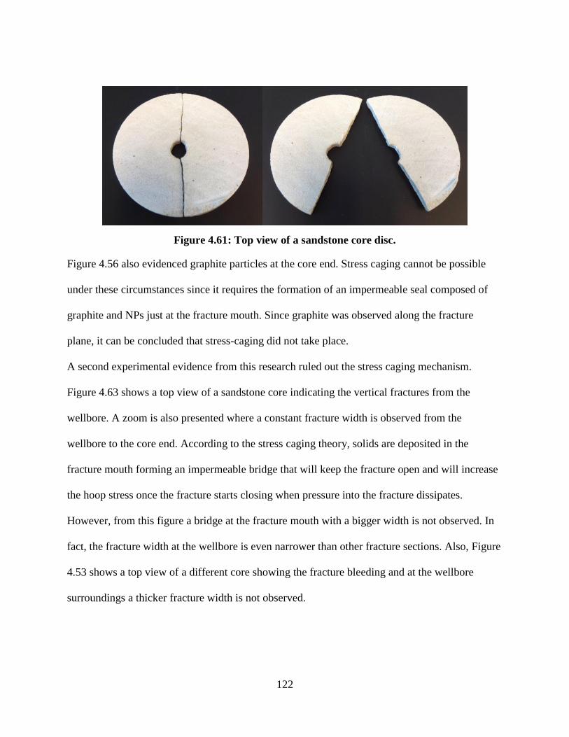
122

Figure 4.61: Top view of a sandstone core disc.

Figure 4.56 also evidenced graphite particles at the core end. Stress caging cannot be possible

under these circumstances since it requires the formation of an impermeable seal composed of

graphite and NPs just at the fracture mouth. Since graphite was observed along the fracture

plane, it can be concluded that stress-caging did not take place.

A second experimental evidence from this research ruled out the stress caging mechanism.

Figure 4.63 shows a top view of a sandstone core indicating the vertical fractures from the

wellbore. A zoom is also presented where a constant fracture width is observed from the

wellbore to the core end. According to the stress caging theory, solids are deposited in the

fracture mouth forming an impermeable bridge that will keep the fracture open and will increase

the hoop stress once the fracture starts closing when pressure into the fracture dissipates.

However, from this figure a bridge at the fracture mouth with a bigger width is not observed. In

fact, the fracture width at the wellbore is even narrower than other fracture sections. Also, Figure

4.53 shows a top view of a different core showing the fracture bleeding and at the wellbore

surroundings a thicker fracture width is not observed.

123

Figure 4.62: Cross-section of sandstone disc along fracture plane. Note the presence of

graphite along the fracture plane.

SEM and EDX analysis were performed on different sections of a sandstone core where wellbore

strengthening with NP2 was conducted. Imaging along the fracture was conducted from the

fracture mouth, middle fracture, and at the fracture end. The samples were obtained from these

locations as illustrated in Figure 4.64. Figure 4.65 shows the sandstone samples and the SEM

device used in the analysis. This was done to confirm the presence of a fracture seal all the way

along the fracture.

(a) (b)

Figure 4.63: (a) Top view of a sandstone core indicating the vertical fractures. (b) Top view

showing the same fracture with along the fracture.

Graphite was observed along the fracture plane

Same fracture width along the core

Vertical fractures

(Top View)

124

Figure 4.66 shows SEM and EDX results from fracture top view at three different locations:

fracture mouth, middle fracture, and fracture end. A fracture seal was observed at the three

locations exhibiting an average thickness of 40 µm.

Figure 4.64: Location and nomenclature of sandstone samples analyzed.

This goes against the stress caging theory considerations. EDX allowed the identification of the

calcium prone regions as a result of NP2 presence on the seal shown as pink color.

(a) (b)

Figure 4.65: (a) Sandstone samples for SEM and EDX analysis. (b) Scanning electron

microscope.

125

A nano-scale image in Figure 4.67 shows NP2 of size ≤150 nm . A much higher resolution

image did not allow an easy visualization due to operational limitations.

Figure 4.66: SEM and EDX of fracture seal along a fracture plane cross-section indicating

the presence of calcium particles.

Fracture mouth

Middle fracture

Fracture end

Seal

Seal

Seal

126

NP2 were observed to form agglomarations that can be vizualized in rounded shapes or as ovals.

NP2 are believed to be of an verage size even lower than 100 nm since CaCO3 crystals were not

observed from these SEM images.

(a) (b)

Figure 4.67: (a) NP2 at seal cross-section. (b) NP2 at fracture plane. Particles highlighted

with red arrows have size ≤150nm.

The occurrence of the chemical reaction that produces NP2 and NaCl was demonstrated by a

mapping of the chemical compounds Ca, Na, and Cl on the fracture seal, the fracture plane and

the filter cake around the wellbore. Figure 4.68 ilustrates the chemical compounds

characterization in contrast to the SEM images. The light blue color represents the NaCl as a

result of mixing of green (Na) and blue (Cl) colors. The pink color indicates the calcium prone

regions with the presence of calcium carbonate. There is a homogeneos distribution of NP2 in

the front view of fracture plane. This analisys explicitly proves the occurrence of the chemical

reaction by the in-situ procedure developed in this research.

The filter cake at the wellbore was characterized to determine the thickness and texture. Figure

4.69 shows a cross-section of the wellbore that allows the quantification of the filter cake in

300 µm. This is a desirable thickness in field operations to avoid stuck pipe and any other

127

implication of thick cakes especially in drilling deviated wellbores. A front view of the filter

cake shows few cracks that are the result of the cake dehydtration as result of exposure to air for

a long period of time (> 2 months). This figure also shows the strong adherence between filter

cake and the rock itself. Gaps between them are not observed. This is an important observation in

spite of the cake dehydration.

Figure 4.68: EDX of Ca, Na, and Cl. Light blue color represents NaCl as a result of green

(Na) and blue (Cl) colors mixing.

Fracture seal

Fracture plane

Filter cake

128

The fractures were filled by NPs and LCM in all their extension. This was concluded by the

analysis of the fracture plane cross-section in a macro and micro-scale. Also, the fracture width

was observed to be the approximately the same along the fracture.

Figure 4.69: Wellbore filter cake cross-section (left) and front view (right).

Stress caging was ruled out as the wellbore strengthening mechanism since it is based on the

stopping of the fracture growth quickly due to the seal it creates just at the fracture mouth.

Indeed this mechanism implies that the shorter the propped length the greater the stress achieved.

From this research a homogeneously sealed fracture was observed. Based on the experimental

results, SEM and EDX, the fracture tip isolation by the development of an immobile mas was

concluded to be the predominant wellbore strengthening mechanism in sandstone cores.

4.9 Summary

Wellbore strengthening was successfully achieved by in-situ prepared NPs on the sandstone

cores used in this research. The Pfb given by the control sample was increased up to 65.1% by

using NP2. This Pfb increase could have a strong impact on drilling and completions operations.

Filter Cake

129

The predominant wellbore strengthening mechanism was identified as the tip isolation by the

development of an immobile mass since according to post-testing analysis the fracture was found

completely sealed from tip to wellbore. A strong match between wellbore strengthening and

filtration at HPHT was found and this could lead to inferences about the physical phenomenon of

the strengthening process. Overall, for a particular NP type, higher filtration was proportionally

associated with a less significant wellbore strengthening. The hypothesis behind this finding

relies on the fact that while it is true that some filtration is required for the carrier fluid to

dehydrate and form an immobile mass into the formation, excessive mud filtration is related to

NPs agglomeration and to the rapid dehydration of the blend while traveling along the fracture. If

this occurs, the particles will not have an effective transport medium to travel and deposit at the

fracture tip.

NP1 blends gave in average less filtration than NP2. However, NP2 blends performed better in

the strengthening experiments. A relationship between these two different phenomena needs to

be conducted carefully and the differences required to be fully understood. First, NP1 and NP2

are different in nature. NP1 are smaller than NP2 and NP2 have a bigger particle size distribution

that could at first glance help for the strengthening process as some authors argue (Van Oort and

Friedheim, 2011; Aston et al., 2004; Alberty and McLean, 2004). Secondly, while the filtration

occurred at constant pressure of 500 psi in a static process, the wellbore strengthening is a

dynamic process that occurred typically at pressures >2000 psi. Finally, NP1 blends have in

average less viscosity than NP2 blends. From this research results, the next hypothesis is drawn

to explain this contrast between filtration and wellbore strengthening between NP1 and NP2.

Since NP1 blends are less viscous and give less filtration, the carrier fluid containing NPs and

graphite will travel fast through the fracture plane generating just small blend dehydration. This

130

will result in a weak seal compared to the seal than is created by NP2 blends. This claim can be

supported by pressure vs. time plots obtained from the hydraulic fracturing experiments. Note in

the P vs t plots for NP1 blends (Figs. 4.42-4.48) that the during the first injection cycle, some

pressure peaks were obtained. However, the Pfb (maximum pressured reached) corresponded to

the first of those peaks. It can be inferred that once a first strong seal was broken, the blend

inside the fracture was unable to create a stronger seal. On the other hand, from the P vs. t plots

for NP2 blends (Figs. 4.31-4.40), the Pfb was recorded not as the first pressure peak. This means

that once a first strong seal was broken, the blend inside the fracture was able to create an even

stronger one. This could have occurred since the NP2 blend traveled slower along the fracture

due to their higher viscosity and the carrier fluid dehydration properly took place giving as a

result stronger seals that led to higher Pfb.

131

Nanoparticles Application for Wellbore Strengthening in Shale Cores Chapter Five:

5.1 Introduction to the Experimental Analysis

Wellbore strengthening in shale cores is a current controversial topic in the drilling industry.

Skeptics believe that this phenomenon cannot occur in shale cores due to its “impermeable”

nature based on the hypothesis that the wellbore strengthening requires a conventional porous

media. Another school of thought (Aston et al., 2007) believes that wellbore strengthening is

feasible in shale formations if a fluid that acts as “cement” can travel along the fracture created

and adhere to the surface. Tests on concrete cores simulating an impermeable media (Nwaoji,

2012) have suggested that wellbore strengthening can in fact take place to a certain degree.

This research presents an original approach based on utilization of in-house prepared NPs and

graphite as wellbore strengthening agents in OBM. Wellbore strengthening in shale formations

was experimentally confirmed in this research. The hypothesis that wellbore strengthening is

related to mud filtration was also tested. The experimental procedures involved conduction of

hydraulic fracturing experiments of a high operational complexity, optical microscopy, SEM and

EDX analysis. Tip resistance by the development of an immobile mass was identified as the

wellbore strengthening mechanism.

The first stage of this research involved sample preparation. Then, an experimental approach was

established since shale cores were not previously tested in the available experimental set-up.

Optimum testing conditions and consideration in the sample preparation were identified and

reported to be used in future works. Calcium-based (NP2) gave a higher performance in

comparison to iron-based (NP1). This same behavior was observed in sandstone cores. Recycled

OBM was compared to a virgin OBM used as the carrier fluid to test NPs performance in this

132

altered (or “dirty”) mud system with higher water content, higher density, and presence of

leftover drill cuttings. Results anticipate that this technology can be extrapolated to field

scenarios.

5.2 Experimental Facilities and Apparatus

Experimental facilities and some apparatus used for sandstone cores preparation and testing were

also used in this research step. In addition , the drill press presented in Figure 5.1 was

incorporated to the shale cores preparation to drill the wellbore. Samples used in Brazilian tests

for determination of tensile strenght were also drilled using this drill press after an appropiate bit

selection. Some attachments were designed and manufacturing to carry out the drilling operation.

Manipulation of shale cores of this size was never done in this institution and an experimental

protocol was developed and will serve in future testing.

Figure 5.1: Drill press at RMERC.

133

5.3 Shale Cores Characterization

5.3.1 Composition

Catoosa shale was used as the impermeable media. Catoosa shale is a Pennsylvanian age, marine

shale (Shewalla, 2007) obtained from Catoosa, Oklahoma. Composition of Catoosa shale is

presented in Table 5-1. This shale is highly sensitive to water and air.

Table 5-1: Catoosa shale composition (Andersen and Azar, 1993).

Mineral %

Quartz 47

Feldspar 9

Calcite Trace

Dolomite 0

Chlorite 15

Illite/Mica 29

Smectite 0

5.3.2 Porosity and permeability

Porosity and permeability are two key rock parameters required for reservoir simulation and also

development of successful drill plans since these parameters are related to the formation stress

analysis (Reyes and Osisanya, 2000). Porosity and permeability vs. confining pressure plots

show the strong effect that compaction has on these properties for different shale formations

(Reyes and Osisanya, 2000). These plots were developed from compaction analysis, porosity

testing models, and design of a small-scale laboratory pressure vessel that simulates downhole

conditions. Figure 5.2 shows a plot of porosity vs. effective stress for Catoosa shale. Note that

the porosity value is reduced when the effective stress is increased.

Figure 5.3 shows a plot of permeability vs. effective stress for Catoosa shale. Note that at

effective stress values >3000 psi the permeability tends to zero. At 400 psi, Figure 5.2 shows a

porosity value of 0.0773 (fraction). Likewise, at the same load of 400 psi, Figure 5.3 shows an

average permeability value of 0.007 md obtained from an extrapolation to the vertical axis as

134

indicated by the red arrows. These values of porosity and permeability at the testing conditions

will be later used in the flow unit’s analysis to infer about fluid filtration into the shale pore

throats.

Figure 5.2: Porosity vs. effective stress for Catoosa shale (Reyes and Osisanya, 2000).

Figure 5.3: Permeability vs. effective stress for Catoosa shale (Reyes and Osisanya, 2000).

135

5.3.3 Tensile strength

Brazilian tests were conducted for the estimation of the tensile strength. Rock samples of 2”x1”

were required. Figure 5.4 shows the set-up for the cores drilling and a shale core after drilling. A

2” core bit was used in a filter press. Wood supports were manufactured and secured using a

chain with a locking plier to avoid vibration.

(a) (b) (c)

Figure 5.4: (a) Core bit, drill press and shale core. (b) Set-up during drilling of 2”x1” cores.

(c) 2”x1” shale core.

Shale cores were drilled parallel and perpendicular to the wellbore direction. This gives a more

robust shale characterization. Figure 5.5 shows the cores used in the Brazilian tests preserved in

mineral oil to avoid any interaction with air which affects their mechanical properties. The shales

cores drilled parallel to wellbore are presented in Figure 5.6 after the Brazilian test. The average

tensile strength was quantified in 90 psi. Figure 5.7 shows the cores drilled perpendicular to the

wellbore after the Brazilian test. An average tensile strength of 65 psi was measured in this

opportunity. It is reasonable for shale formations that the tensile strength of samples containing

the layers horizontally to the direction of the load gives a lower value of tensile strength.

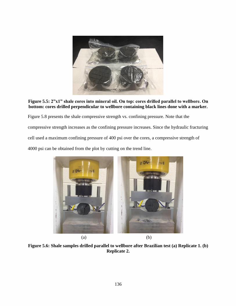
136

Figure 5.5: 2”x1” shale cores into mineral oil. On top: cores drilled parallel to wellbore. On

bottom: cores drilled perpendicular to wellbore containing black lines done with a marker.

Figure 5.8 presents the shale compressive strength vs. confining pressure. Note that the

compressive strength increases as the confining pressure increases. Since the hydraulic fracturing

cell used a maximum confining pressure of 400 psi over the cores, a compressive strength of

4000 psi can be obtained from the plot by cutting on the trend line.

(a) (b)

Figure 5.6: Shale samples drilled parallel to wellbore after Brazilian test (a) Replicate 1. (b)

Replicate 2.

137

(a) (b)

Figure 5.7: Shale samples drilled perpendicular to wellbore after Brazilian test (a)

Replicate 1. (b) Replicate 2.

Figure 5.8: Compressive strength of Catoosa shale at various confining pressures

(Andersen and Azar, 1993).

5.4 Shale Cores Preparation

53/4

”x 9” shale cores were provided in plastic pipes. Each pipe contained 4 cores with bubble

wrap as illustrated in Figure 5.9. The shale core preparation followed the next steps:

138

Removing of bubble wrap

Placement into mineral oil (Figure 5.9)

Drilling of 9/16” wellbore in the center of the cores

Casing assembly on steel caps and cementing of caps in cores

Cement dry out

Core surface grinding

Post-testing caps cleaning

These core preparation steps take a minimum of 3 days assuming that all the steps are carried out

consecutively. In other case, the cores need to be placed into mineral oil to avoid contact with

air. The key steps in the core sample preparation are described as follows.

(a) (b)

Figure 5.9: (a) Wrapped shale core. (b) Shale cores into mineral oil. (c) Shale core with a

mineral oil film exposed to air.

5.4.1 Drilling of 9/16” wellbore in the center of the cores

Drilling of the wellbore in the center of the shale core was conducted with a 9/16” steel twist

drill bit using a drill press as shown in Figure 5.10. The drilling operation was carried out in dry.

139

Intervals of 1” were drilled gradually pulling the bit out of the core and cleaning it with air at 60

psi. This was required to cool the bit down since temperature increases rapidly while drilling.

Figure 5.10: Shale core on drill press table for wellbore drilling. A 9/16” steel twist drill bit

was used for drilling.

The set-up for the wellbore drilling is presented in Figure 5.11. Wood supports were

manufactured to be used at the guide surroundings and secured using a locking plier at pressure

to avoid vibration. Half the core is drilled and then the core is flipped to drill the other end. This

will ensure a centered wellbore. Drill cuttings obtained while drilling are also shown.

5.4.2 Casing assembly on steel caps and cementing of caps in cores

The same steel caps and casing used in sandstone core preparation were used for shale cores.

Preparation of the epoxy followed the same procedure described in the previous chapters.

However, the cementing procedure itself differs in the fact that the shale core needs to be

wrapped to avoid contact to air. Plastic wrap was used around the core leaving only the top and

bottom end in contact with the epoxy. Three clamps with 120° between them were used to ensure

the attachment of the epoxy on the shale surface.

140

(a) (b)

Figure 5.11: (a) Set-up for wellbore drilling. (b) Wellbore drilling. Note the drill cuttings

from drilling on the wood guide.

5.4.3 Cement dry out

Figure 5.12 shows the drying out of a shale and sandstone core. Note that the shale core is

completely wrapped to avoid contact with air. After 24 hours of first cap dry out, the same

procedure is done on the other end. Note that the wellbore needs to be sealed with tape to avoid

air into the wellbore.

Figure 5.12: Cementing of shale cores. Note that the core is wrapped to avoid contact with

air. A contrast with a sandstone core cementing is illustrated.

141

Figure 5.13 shows shale cores after the cement dry out. The cores are wrapped with plastic and

tape is used at the top and bottom as illustrated. The core surface grinding was carried out using

basically the same procedure for sandstone cores. The only difference is that for shale cores the

core was kept vertical during the grinding to avoid core deterioration by rotation. The cap

cleaning was also a step in core preparation. In this case the procedure was easier than for

sandstone cores as the shale formation exhibits a plastic behavior and gets weakened by exposure

to air.

Figure 5.13: Shale core wrapped after cementing and prior to hydraulic fracturing test.

5.5 Challenges Faced and Solutions in Shale Cores Preparation

The shale cores preparation is a complex task since this type of rock is very sensitive to air and

water. In each core preparation step, a careful isolation of the sample was conducted. Once shale

contacts either air or water its mechanical properties are affected and therefore the test results

can be bias. The key challenges in the core preparation for the wellbore strengthening tests were:

142

Drilling of wellbore in the center

Steel caps cementing

A brief description of the challenge and solution follows this discussion.

5.5.1 Drilling of wellbore in the center

Drilling of the wellbore in the center of the shale cores was a subject of discussion for the

research team. The first attempt was carried out using the same approach of sandstone cores. The

rock drill was used with a 9/16” diamond insert bit in dry. Water was not pumped through the

annular to avoid interaction with the shale. After 2” of drilled depth, the bit became hot to the

point that a significant amount of smoke was experienced. At this point, a regular diamond insert

bit was ruled out. A next approach involved the use of a drill press as presented in Figure 5.1.

The next step was the bit selection. Since the shale exhibited a soft texture a 9/16” wood bit was

used. The bit drilled relatively fast for the first 2” and suddenly got stuck into the core. The core

rotated along with the bit until the bit broke and the core fell to the floor at approximately 2 m

from the drill press. Figure 5.14 shows the broken bit. This was due to excessive heating of the

bit and poor well cleaning by an inefficient drill cuttings removal. This situation required an

investigation about an optimum bit to drill this type of hole in a shale core. The first aspect

considered was the well cleaning. A bit with bigger channels is required for a better cuttings

transport to the surface. Also a bit with higher resistance to temperature ensured more stability

while drilling in dry. Finally, the drilling should be performed in depths intervals of 1” followed

by removing the bit from the wellbore and applying air to cool it down. A steel twist drill bit was

selected as presented in Figure 5.10. This bit has much bigger channels and higher resistance.

With this bit the drilling of straight wellbores was carried out without complications.

143

Figure 5.14: Wood bit broken in two pieces.

5.5.2 Steel caps cementing

The challenge on the steel caps cementing in shale cores relies on the core protection to avoid

contact with air or water. A careful wrapping of the core was conducted leaving only 1” of core

exposure close to the steel cap. This exposed surface will be covered with cement for later

grinding. The interface between the cement and the steel cap needs to be smooth to allow an

evenly applied confining pressure. The wellbore on the core and on the steel caps were covered

with tape to avoid air entrance into the wellbore. The surface grinding was conducted carefully

with the core in a vertical position. Only the area close to the steel caps required grinding.

5.6 Wellbore Strengthening Tests using a Hydraulic Fracturing Apparatus

5.6.1 Experimental procedure for testing of shale cores

The hydraulic fracturing tests in shale cores are conducted basically in the same way as that for

sandstone cores. The key differences compared to the check list of Table 4-4 in a previous

chapter are listed below:

Plastic wrap on the shale core is removed after screwing the injection line into the sample

(Step 10). This is due to avoid as much as possible the core contact with air

144

Before placing the core into the pressure cell (Step 9) a tape surrounding the bottom end

of the core is manufactured to place the core into the pressure cell. This is done to avoid

axial tension on the core that could cause failure

Blend preparation is carried out before the overburden load and confining pressure

application (Steps 28-31). Overburden is applied slowly until 350 psi. This type of shale

cores are sensitive to the rate at which the load is applied. 100 psi/min is an advisable rate

The check list post-experiment follows the same steps from Table 4-5.

5.6.2 Wellbore strengthening results

Based on filtration and wellbore strengthening results from sandstone cores, an optimized test

schedule for shale cores was developed. This schedule allowed the understanding of the two

different types of NPs in shale cores. The wellbore strengthening mechanism was identified from

this testing. Two different mud systems were tested, virgin OBM and recycled OBM provided

by Blackstone from the field. The virgin OBM (90:10) was the same used in filtration

experiments and wellbore strengthening tests in sandstone cores. The recycled OBM (87:13) was

obtained from a depth of 2929 m with higher water content and density (1100 kg/m3 vs. 926

kg/m3). A higher plastic viscosity (20 cp), yield point (6 lb/100ft

2) and gel strength at 10 min (11

lb/100ft2) compared to the virgin mud was recorded. Drill cuttings were also observed in the

recycled sample. The use of a recycled mud created a strong impact on these research results by

quantifying the NPs performance in a “dirty” OBM sample.

The tests conducted in virgin OBM included the control sample, DF1, DC6, DC4, and DF3

blends. Table 4-7 shows the concentration levels for each blend. The most remarkable data

obtained from the hydraulic fracturing experiments for these blends is described next. Results

analysis and implications will be later addressed in an independent section.

145

Control Sample (CS) Test

The Pfb for the control sample (sample without NPs and graphite) was 519.6 psi. Figure 5.15

shows the P vs. t plot. After 10 min of fracture healing, the maximum pressure recorded was

497.8 psi. In contrast to the tests on sandstones, refilling of the syringe pumps was not required

before the first fracture propagation. This is due to the low permeability of the shale that prevents

mud filtration.

Figure 5.15: P vs. t plot for control sample in shale.

Figure 5.16 shows the shale core after the testing. Mud bleeding through the fracture was

observed.

Figure 5.16: Core after control sample in shale testing.

146

DC4 Shale

An initial breakdown pressure of 519.9 psi was recorded. After fracture healing of 10 min, the

maximum pressure recorded in the second injection cycle reached 659.3 psi as illustrated in

Figure 5.17. This means a 26.9% of strengthening in comparison to the control sample. The core

after the test is presented in Figure 5.18.

Figure 5.17: P vs. t plot for DC4 Shale indicating the pressure increase.

Note that in the core two vertical fractures are observed. This is consistent with the P vs. t plot

and indicates that the wellbore was strengthened in the direction of the initial fracture and the

fluid from the second injection cycle was forced to follow a different direction.

DC6 Shale

Figure 5.19 shows the pressure behavior for the DC6 blend. An initial breakdown pressure of

502.9 psi was recorded. This value is similar to the control sample. A similar situation

experienced with DC4 was observed.

26.9% increase

147

Figure 5.18: Core after DC4 Shale testing.

The maximum pressure obtained in the second injection cycle reached 673.9 psi, giving this a

29.7% increase in wellbore strengthening compared to the control sample. The performance of

DC6 was slightly better than for DC4. This same situation was observed in testing of sandstone

cores.

Figure 5.19: P vs. t plot for DC6 Shale indicating the pressure increase.

29.7% increase

148

Figure 5.20: Core after DC6 Shale testing.

Figure 5.20 shows the core after the DC6 blend testing. Two vertical fractures are visualized.

This means that wellbore strengthening took place after the first injection cycle and fracture

healing.

Figure 5.21: P vs. t plot for DF1 Shale indicating the pressure increase.

20% increase

149

DF1 Shale

DC1 blend was tested in a shale core and Figure 5.21shows the pressure behavior. A maximum

pressure of 625.84 psi was recorded after the second injection cycle. This represents 20% of

wellbore strengthening. The initial breakdown pressure was quantified in 523.74 psi. This value

is basically the same as the control sample. Figure 5.22 shows the core after the testing. Two

bleeding vertical fractures were observed.

Figure 5.22: Core after DF1 Shale testing.

DF3 Shale

Figure 5.23 shows the P vs. t plot for the DF3 blend. A maximum pressure of 552 psi was

reached after the second injection cycle. This pressure increase gives 6.3% wellbore

strenghtening. The initial breakdown pressure was quantified in 524 psi. Overall, the

performance of NP2 on wellbore strengthening is better than NP1 on virgin OBM. The same

happened in sandstone cores. Figure 5.24 shows the core after testing. Two verical fractures were

observed. This allows concluding that with virgin OBM a second vertical fracture is forced to

follow a different direction.

150

Figure 5.23: P vs. t plot for DF3 Shale indicating the pressure increase.

Testing of strengthening in shale cores also involved recycled OBM. The summary of each

conducted test is presented as follows starting from the test involving the control sample of

recycled mud.

Figure 5.24: Core after DF3 Shale testing.

6.3% increase

151

Control Sample (CS) test on recycled mud

Figure 5.25 shows the mixing of the recycled mud (without NPs and graphite) before the testing.

The pressure behaviour in time is presented as Figure 5.26. A maximum pressure increase of

485.6 psi was recorded. This is similar value to the CS for virgin mud (519.6 psi), i.e., a

difference of just 7%. This value will serve as reference to calculate the wellbore strengthening.

After 10 min of fracture healing, a maximum pressure of 360 psi was recorded in the second

injection cycle.

Figure 5.25: Mixing of recycled mud for testing.

Figure 5.27 shows the core after the testing indicating a vertical fracture.

Figure 5.26: P vs. t plot for Blackstone control sample in shale.

152

Figure 5.27: Core after Blackstone control sample testing.

BDF-B3-I-05A

This blend contains 0.5 wt% of Iron NPs prepared in-situ from aqueous precursors. 0.5 wt% of

graphite was also added. 534.98 psi was recorded as the maximum pressure. This gives 10% of

wellbore strengthening compared to the control sample. Figure 5.28 shows the P vs. t plot. The

core after testing is presented in Figure 5.29.

Figure 5.28: P vs. t plot for BDF-B3-I-05A indicating the pressure increase.

10% increase

153

In contrast to DF1, which also has NP1 at 0.5 wt%, this blend BDF-B3-I-05A did not perform

that good. Giving this an insight that NP1 work more effectively on virgin mud.

Figure 5.29: Core after BDF-B3-I-05A testing.

BDF-B3-I-05C

This blend also contains a 0.5 wt% of NP1 and 0.5 wt% of graphite. NP1 preparation differed

from the blend BDF-B3-I-05A. The NP1 preparation consisted of mixed the recycled mud with a

virgin OBM containing a high NP1 concentration of 5 wt% in a 90:10 proportion. A maximum

pressure increase of 529 psi was recorded. This gives an 8.4% of wellbore strengthening. It is

concluded that the way NP1 is prepared does not have a significant impact on strengthening.

Figure 5.30 shows the P vs. t plot. The initial breakdown pressure was 488.1 psi. Figure 5.31

shows the core after the testing showing two vertical fractures.

BDF-B3-C-3S

This blend contains 3.0 wt% of NP2 and 2.0 wt% of graphite. 627.7 psi was recorded as the

maximum pressure after the second injection cycle. This represents 29.2% of wellbore

strengthening. The initial breakdown pressure was quantified as 484.7 psi. Figure 5.32 shows the

154

P vs. t plot. DC6 blend gave 29.7 % of wellbore strengthening. From this it can concluded that

recycled mud does not have a big effect on NP2 performance.

Figure 5.30: P vs. t plot for BDF-B3-I-05C indicating the pressure increase.

The core after testing is presented in Figure 5.33 showing two vertical fractures.

Figure 5.31: Core after BDF-B3-I-05C testing.

8.4% increase

155

0.5 wt% of Graphite in recycled mud

From tests in sandstone cores it was concluded that the graphite level is not a critical parameter

for wellbore strengthening when NPs are not added to blends. A blend just containing graphite at

0.5 wt% was tested in a shale core to have a reference point at 0 wt% of NPs concentration.

Figure 5.32: P vs. t plot for BDF-B3-C-3S indicating the pressure increase.

Figure 5.34 shows the P vs. t plot where a very small pressure increase over the control sample

was experienced.

Figure 5.33: Core after BDF-B3-C-3S testing.

29.2% increase

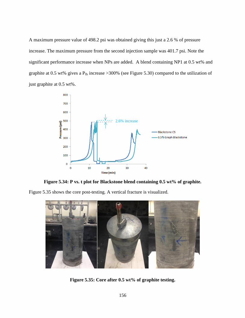
156

A maximum pressure value of 498.2 psi was obtained giving this just a 2.6 % of pressure

increase. The maximum pressure from the second injection sample was 401.7 psi. Note the

significant performance increase when NPs are added. A blend containing NP1 at 0.5 wt% and

graphite at 0.5 wt% gives a Pfb increase >300% (see Figure 5.30) compared to the utilization of

just graphite at 0.5 wt%.

Figure 5.34: P vs. t plot for Blackstone blend containing 0.5 wt% of graphite.

Figure 5.35 shows the core post-testing. A vertical fracture is visualized.

Figure 5.35: Core after 0.5 wt% of graphite testing.

2.6% increase

157

5.6.3 Challenges faced in wellbore strengthening tests

Wellbore strengthening tests on shale cores are complex. Especially since these types of

formations were not tested previously in the hydraulic fracturing apparatus. The first research

step in shale tests involved finding the optimum operational parameters for a successful test. In

this section, the most relevant challenges faced are addressed and the lessons learned are

highlighted for future reference. This research involved troubleshooting of all the experimental

issues from the experimental testing. Just a limited contribution from mechanical technicians was

received.

Core failure when applying overburden load

In the third test, the core failed when applying overburden load at an approximate pressure of

380 psi. The rate at which the overburden load was applied followed the same approach from the

previous two cores. This was also the same approach used in applying the overburden load to the

sandstone cores. When the core failed the overburden load decreased rapidly to 50 psi. At this

time the load was removed and the core was extracted from the pressure cell. Figure 5.36 shows

the core taken out from the pressure cell and a view of the inside of the pressure cell. The

removal of the shale cores segments from the pressure cell is a tedious activity that required the

use of a hand drill to break it into small segments to allow easy manual extraction. This removal

needs to be conducted carefully to avoid deterioration of the rubber sleeve that applies confining

pressure. A chisel and a hammer were initially used but it took considerable time.

158

(a) (b) (c)

Figure 5.36: (a) Shale core from top cap after failure. (b) Shale core from top and bottom

cap after failure. (c) Shale segments inside pressure cell.

When the overburden load and steel caps over the broken core were removed, water droplets

were observed. This indicated that water leakage occurred from the confining rubber sleeve due

to the test failure. After all the shale segments were removed, the cause of the leakage was

investigated. A leakage test involved air injection at 60 psi through the confining line and

bubbles and air coming out were observed in the area highlighted in Figure 5.37.

Figure 5.37: Rubber sleeve after shale core segments extraction. Red arrow indicates the

leakage area.

When the core fails, sliding of the top part of the core occurs along the failure plane and this

exerts a high pressure on the rubber sleeve until the point of breaking the silicon seal. As

previously mentioned, this research also involved troubleshooting of this issue. For solving the

Leakage

159

leakage, the pressure cell required disassembly. The pressure cell-disassembly and assembly

consists of the next steps:

- Unscrew of nuts from top flange

- Rods removing from top flange (it required hammering downwards)

- Removing of top flange by hammering using a sledgehammer

- Removing of rubber sleeve (Figure 5.38a)

- Raising of steel cell using cell motors (Figure 5.38b)

- Cleaning old silicon. Removing of gaskets

- Placing of a new bottom gasket and silicon. Placement of a new rubber sleeve on bottom

flange and into the steel cell (Figure 5.38c)

- Placement of top flange

- Tightening nuts on rods

- Silicon dry out for 24 hours

Once the cell was assembled, a leakage test was conducted by filling the pressure cell with water

and injecting air to the confining rubber sleeve. If bubbles coming out from the sleeve were not

observed, the system was ready for a new test. This complete procedure takes a total of 2 days if

there is availability of rubber sleeves and gaskets.

Second core failure when applying overburden load

After the test failure, two main reasons were considered as the root cause. Excess of overburden

pressure applied on the shale core and failure due to axial tension were considered. A new

approach for pressurizing the shale core into the pressure shale was conducted:

- Apply overburden pressure up to 100 psi

- Apply confining pressure up to 100 psi

160

- Increase pressure in the wellbore up to 100 psi

- Increase overburden pressure up to 400 psi

(a) (b) (c)

Figure 5.38: (a) Rubber sleeve. (b) Steel cylinder removal from bottom flange. (c)

Placement of a new rubber sleeve and silicon.

To avoid the failure due to axial tension, a tape support for the bottom cap was manufactured as

illustrated in Figure 5.39a. This allowed the placement of the core into the pressure cell by

supporting it from the tape. The steel caps weight is 1 kg and if the core is placed into the

pressure cell from supporting the top cap this weight may be responsible of the failure due to

tension load. Using this new approach the overburden load was increased to 380 psi. At that

point the core failed and the confining gauge showed a pressure increase up to 200 psi. This

confining pressure increase occurred due to the pressure exerted by the broken core towards the

rubber sleeve. Figure 5.39b shows a top view of the pressure cell where the height reduction is

observed due to the breaking. Figure 5.39c shows the shale core after extraction from the

pressure cell.

161

(a) (b) (c)

Figure 5.39: (a) Tape support for bottom cap. (b) Top view of pressure cell after core

failure. (c) Shale core after failure.

Third core failure when applying overburden load

After the second failed test, a maximum overburden pressure of 350 psi was applied.

Investigation of the failure led to the conclusion that shale cores were experiencing a certain

degree of strength reduction due to contact with mineral oil. The overburden stress reduction will

not have any effect on the fracture gradient since this is not a parameter involved in the fracture

gradient estimation in this type of system. The original approach of applying first overburden

pressure and then confining was used. When the pressure in the overburden gauge reached 350

psi the core failed and immediate reduction of overburden pressure was experienced.

Figure 5.40 shows the pressure cell and shale core after failure. From this point the maximum

overburden load to be applied in further tests was evaluated. Also, the rate at which the

overburden rate was applied was considered.

162

(a) (b)

Figure 5.40: (a) Top view of pressure cell after core failure. (b) Shale core after failure.

Test failure due to leakage from confining rubber sleeve

From the bulk of failed experiments, two new steps were established:

- Apply overburden load up to 350 psi

- Use a load rate of 100 psi/min instead of 300 psi/min as in the previous experiments

The failure of the cores while applying the overburden load was assumed to take place not only

due to high stress values but also the rate at which the stress was applied.

This approach was successfully carried out in a fourth experiment. The core did not break with

an applied overburden load of 350 psi. It was concluded that an optimum load application rate

was found. However, when the confining pressure was applied a water leak was observed and

illustrated in Figure 5.41. This water escaped from the rubber sleeve due to a broken silicon seal.

This silicon seal was affected after the failure of the third core. In conclusion, every time a core

fails, a complete cell disassembly needs to be done to set new gaskets and silicon seals.

163

(a) (b)

Figure 5.41: (a) Top view of pressure cell before testing. (b) Water leakage from rubber

sleeve on top pressure cell.

In this case the pressure disassembly and assembly was even more challenging. The gaskets

needed for the bottom flange were no longer available. The use of a new bottom gasket was

required. Note in Figure 5.42 the difference between the top and bottom gasket. A gasket of this

dimension (8.5”ODx8.0”IDx0.25”) was not available. This required the manufacturing of a

gasket of this dimension from a SBR rubber strip shown in Figure 5.42. A compass cutter knife

was used in the shop to obtain the desired dimensions. Figure 5.43 showed the in-house

manufactured gasket at the bottom flange. For the top flange the same top gasket that was in

good conditions was used.

Water

164

(a) (b)

Figure 5.42: (a) Top and bottom gaskets. (b) SBR rubber strip for gasket manufacturing.

This endeavor took a total of 5 days from the arrival of the SBR strip. This new assembly

worked successfully for the upcoming tests. The new overburden load values and rate of

application were considered.

Figure 5.43: New gasket on bottom flange.

Top Gasket Bottom Gasket

New Gasket

165

5.7 Shale Cores Post-testing Analysis

After removing the steel caps a cross-section of the core can be visualized. Figure 5.44 shows a

cross-section where the vertical fracture can be observed. Note that more than two vertical

fractures are present. This corroborated the strengthening in the direction of the original fracture

and the creation of a second hydraulic fracture in a different direction as a result of the second

injection cycle.

Figure 5.44: Shale core after testing. A vertical fracture can be observed.

A Hirox Optical Digital microscope was used to take a picture of the fractures in the shale core

after the hydraulic fracturing test. Figure 5.45 shows a zoom on the two vertical fractures

obtained from the core presented in Figure 5.22. The fracture width had an average value of

20 µm. This same average fracture width was recorded along the fracture. Figure 5.46 shows the

shale disc that was used in this analysis. This disc was cut from the shale core using the rock saw

at the RMERC. Cutting was performed in dry since this formation is sensitive to water. The other

end of the disc was taped to avoid disintegration while cutting.

Figure 5.47 shows a zoom of the wellbore where the two horizontal fractures are indicated with

red arrows. A 3D recreation of wellbore was developed. Two vertical fractures can also be

observed from this perspective.

166

(a) (b)

Figure 5.45: (a) Core showing two vertical fractures. (b) Hirox Optical Digital microscope

on shale sample.

A microscope analysis was also conducted at the core end. Figure 5.48 shows a microscope

image of the hydraulic fractures at the core end. An average fracture with of 20 µm was also

observed at the core end. A 3D of the core end was also conducted and allows visualizing of the

fracture path at the core end.

Figure 5.46: Top view of shale sample analyzed in Optical microscope.

167

A constant fracture width along the fracture plane is an important implication for the

understanding of the wellbore strenghtening mechanism. This will be addressed in the next

section.

Figure 5.47: (a) Shale core wellbore indicating two vertical fractures. (b) 3D illustration of

shale core wellbore.

Figure 5.48: (a) Shale core end indicating two vertical fractures. (b) 3D illustration of shale

core end.

168

5.8 Results Analysis and Proposed Mechanism for Wellbore Strengthening in Shale Cores

5.8.1 Results analysis of wellbore strengthening in shale cores

Wellbore strengthening results for NP2 are summarized in Figure 5.49. This plot includes the

tests results from the virgin OBM and the recycled sample. Note a defined trend was obtained

which resembles the trend obtained for NP2 in sandstone cores. At NP2 concentrations <0.5 wt%

there was a rapid increase in Pfb as concentration increases. At concentrations >0.5 wt%, further

addition of NP2 just slightly helped the strengthening process. Despite two different fluids were

included in this plot, a trend was observed. This indicates that the performance of NP2 was not

susceptible to higher water content, density and presence of drill cuttings.

Figure 5.49: % Pfb vs. NP2 concentration in shale cores.

Results obtained from NP1 contained blends are summarized in Figure 5.50. Blends prepared

from virgin and recycled OBM samples were considered. Note that the plot composed by DF1

and DF3 resembled the plot obtained in sandstone cores from NP1 blends. NP1 concentrations

>0.5 wt% negatively affected the wellbore strengthening. Lines connect the Blackstone blends

with the DF3. This was performed as an approximate extrapolation based on the results obtained

with NP2 blends. With NP1 blends, a bigger difference in wellbore strengthening compared to

169

NP2 was observed at 0.5 wt%. The virgin OBM performed slightly better than the recycled

samples. However, it should be pointed out that NPs were prepared from aqueous precursors in

recycled OBM samples. In this way of reasoning, the extrapolations drawn with lines showed

the same trend: at higher NP1 concentration, a worse wellbore strengthening was obtained. This

is a reasonable conclusion since the strengthening obtained is better with virgin mud, so %Pfb at

high NP1 concentration from a recycled mud is not expected to be higher than the one for DF3.

Figure 5.50: %Pfb increase vs. NP1 concentration in shale cores.

A comparison between the wellbore strengthening and filtration results at HPHT for NP2 as a

function of NPs concentration is presented in Figure 5.51. Proportionality between the two

parameters is observed. This means that in shale formation, the amount of filtration towards the

formation has implications on wellbore strengthening performance as occurred with sandstone

cores. This is reasonable since filtration needs to be controlled for the wellbore strengthening

mechanism to take place.

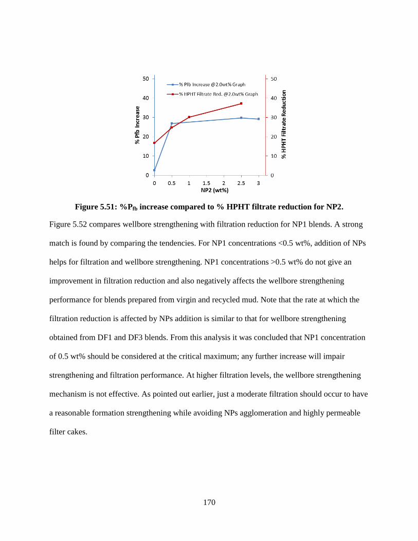
170

Figure 5.51: %Pfb increase compared to % HPHT filtrate reduction for NP2.

Figure 5.52 compares wellbore strengthening with filtration reduction for NP1 blends. A strong

match is found by comparing the tendencies. For NP1 concentrations <0.5 wt%, addition of NPs

helps for filtration and wellbore strengthening. NP1 concentrations >0.5 wt% do not give an

improvement in filtration reduction and also negatively affects the wellbore strengthening

performance for blends prepared from virgin and recycled mud. Note that the rate at which the

filtration reduction is affected by NPs addition is similar to that for wellbore strengthening

obtained from DF1 and DF3 blends. From this analysis it was concluded that NP1 concentration

of 0.5 wt% should be considered at the critical maximum; any further increase will impair

strengthening and filtration performance. At higher filtration levels, the wellbore strengthening

mechanism is not effective. As pointed out earlier, just a moderate filtration should occur to have

a reasonable formation strengthening while avoiding NPs agglomeration and highly permeable

filter cakes.

171

Figure 5.52: % Pfb increase vs. % HPHT filtrate reduction for NP2. Arrow indicates the

direction of NP1 concentration increase.

5.8.2 Proposed mechanism for wellbore strengthening in shale cores

For a better understanding of the wellbore strengthening mechanism in shale cores,

determination of whether the carrier fluid containing NPs and LCM can or cannot enter into the

shale pore throat apertures is required. Some skeptical drilling experts believe that wellbore

strengthening cannot occur in shale formations since invasion of the carried fluids towards the

formation cannot take place. This occurs since drilling is still strongly influenced by empirical

thoughts that consider shale formation as an impermeable media. This research presents

scientific evidence that shows that carrier fluid invasion can occur. This conclusion is based on

shale pore throat apertures calculation as a function of confining pressure. This was corroborated

with SEM analysis that showed a well-established seal composed of NPs and granular material

resembling a filter cake.

NP2 have an average size of 60 nm and have a wide size range from 20 to 500 nm. This wide

particle size distribution makes much more effective fracture sealing since it facilitates

agglomeration and settlement of NPs one over the others. This strong seal created by NP2

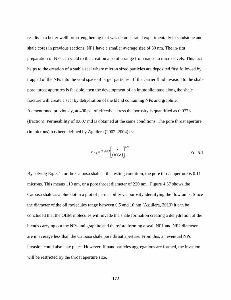
172

results in a better wellbore strengthening that was demonstrated experimentally in sandstone and

shale cores in previous sections. NP1 have a smaller average size of 30 nm. The in-situ

preparation of NPs can yield to the creation also of a range from nano- to micro-levels. This fact

helps to the creation of a stable seal where micron sized particles are deposited first followed by

trapped of the NPs into the void space of larger particles. If the carrier fluid invasion to the shale

pore throat apertures is feasible, then the development of an immobile mass along the shale

fracture will create a seal by dehydration of the blend containing NPs and graphite.

As mentioned previously, at 400 psi of effective stress the porosity is quantified as 0.0773

(fraction). Permeability of 0.007 md is obtained at the same conditions. The pore throat aperture

(in microns) has been defined by Aguilera (2002, 2004) as:

Eq. 5.1

By solving Eq. 5.1 for the Catoosa shale at the testing condition, the pore throat aperture is 0.11

microns. This means 110 nm, or a pore throat diameter of 220 nm. Figure 4.57 shows the

Catoosa shale as a blue dot in a plot of permeability vs. porosity identifying the flow units. Since

the diameter of the oil molecules range between 0.5 and 10 nm (Aguilera, 2013) it can be

concluded that the OBM molecules will invade the shale formation creating a dehydration of the

blends carrying out the NPs and graphite and therefore forming a seal. NP1 and NP2 diameter

are in average less than the Catoosa shale pore throat aperture. From this, an eventual NPs

invasion could also take place. However, if nanoparticles aggregations are formed, the invasion

will be restricted by the throat aperture size.

45.0

35100

665.2

krp

173

Figure 5.53: Permeability vs. Porosity cross-plot including shale formations from Canada

and United States. Nikanassin tight gas formation data is also included and represented on

the top of the plot (Aguilera, 2013). The Blue square stands for the Catoosa shale at testing

conditions.

The disc presented in Figure 5.46 was divided in two pieces and a cross-section that allows

visualizing the fracture plane is presented in Figure 5.54. From this cross-section no details of

the seal formed along the fracture or filter cake around the wellbore can be observed. Since the

sample contains mineral oil on the surface, graphite particles are difficult to observe due to the

dark color. A detailed analysis of the fracture plane and characterization of the seal formed along

the fracture required utilization of SEM analysis.

Figure 5.54: Shale core cross-section along the fracture plane.

1 cm

174

SEM and EDX analysis were performed on a shale core where NP1 nanoparticles were used for

wellbore strengthening. Shale samples at fracture mouth and at the fracture end as shown in

Figure 5.55 were analyzed. Figure 5.56 shows the shale samples prepared for the SEM analysis.

Samples at fracture mouth, at the fracture end, and samples oriented to allow a front view of the

fracture plane were prepared. Cross-section images of the fracture allowed the characterization

of the seal and imaging of the fracture plane itself from a front view allowed the analysis of the

NPs and LCM distribution.

Figure 5.55: Location and nomenclature of shale samples analyzed.

A cross-section analysis of the fracture plane at fracture mouth shows that the thicker seal

measures 20 µm. Figure 5.57 shows the interface between the shale and the seal. It also shows a

zoom on the seal and interface between the seal and the rock. Note that a particle distribution is

observed. Good attachment from the seal towards the formation is also noticed.

This seal dimension matches with the microscope analysis carried out post-testing illustrated in

Figure 5.45. This seal was developed as the carrier fluid invaded the shale formation.

175

Figure 5.56: Shale samples for SEM and EDX analysis.

Figure 5.58 shows an image of much higher resolution allowing the visualizing of the NP1 at the

nano-scale. NP1 are the particles that exhibit brighter color in the image. Some of them have

sizes even smaller than 100 nm.

(a) (b)

Figure 5.57: (a) Cross-section of fracture plane (2000x mag) close to wellbore. (b) Zoom in

seal (5000x mag) at fracture mouth.

A key analysis was carried out by analyzing a fracture plane cross-section at the fracture end.

The images in Figure 5.59 demonstrate that a seal exists at the fracture end. This analysis rules

Shale Seal

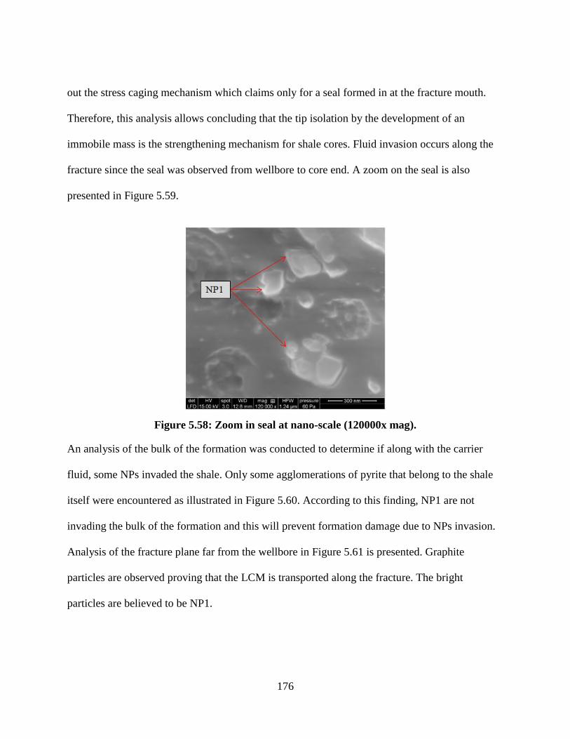
176

out the stress caging mechanism which claims only for a seal formed in at the fracture mouth.

Therefore, this analysis allows concluding that the tip isolation by the development of an

immobile mass is the strengthening mechanism for shale cores. Fluid invasion occurs along the

fracture since the seal was observed from wellbore to core end. A zoom on the seal is also

presented in Figure 5.59.

Figure 5.58: Zoom in seal at nano-scale (120000x mag).

An analysis of the bulk of the formation was conducted to determine if along with the carrier

fluid, some NPs invaded the shale. Only some agglomerations of pyrite that belong to the shale

itself were encountered as illustrated in Figure 5.60. According to this finding, NP1 are not

invading the bulk of the formation and this will prevent formation damage due to NPs invasion.

Analysis of the fracture plane far from the wellbore in Figure 5.61 is presented. Graphite

particles are observed proving that the LCM is transported along the fracture. The bright

particles are believed to be NP1.

177

(a) (b)

Figure 5.59: (a) Cross-section of fracture plane (150x mag) far from wellbore. (b) Zoom in

seal (10000x mag) at fracture end.

A further analysis focused on the NPs distribution in the seal cross-section. Figure 5.62 shows

SEM and EDX images of the seal cross-section. The green color indicates presence of iron

particles. A homogeneous distribution of iron particles along the seal was observed.

Figure 5.60: Bulk of shale (2500x mag) only showing some pyrite agglomerations.

Seal Shale

Pyrite

178

(a) (b)

Figure 5.61: Fracture plane image far from wellbore at (a) 600x mag and (b) 2400x mag.

Note graphite presence far from wellbore.

(a) (b)

Figure 5.62: (a) Seal cross-section (500x mag). (b) EDX of seal cross-section (500x mag).

Green color indicate iron particles distribution on seal.

5.9 Summary

Wellbore strengthening was possible by the implementation of in-situ prepared NPs on shale

cores. Pfb was increased up to 30% by blends containing NP2. Overall, the performance of NP2

Graphite Graphite

179

blends on the tests was superior to those ones composed by NP1. This same conclusion was

obtained from tests conducted on sandstone cores and this allows the generalization that NP2 are

a successful wellbore strengthening agent for sandstone and shale formations. Optical

microscopy, SEM and EDX analysis concluded that the fractures were completely sealed from

tip to wellbore with a homogeneous width. The mass that sealed the fracture resulted from some

(eventually low) fluid invasion towards the formation. This was anticipated to occur based on

rp35 analysis following the approach proposed by Aguilera (2002, 2004). This ruled out the stress

caging as the predominant wellbore strengthening mechanism. A comparison between wellbore

strengthening and filtration reduction trends showed that proportionality exists between these

two parameters, and therefore the physical mechanism of wellbore strengthening in shale can be

related to the previous one discussed for sandstone in Chapter 4. Based on experimental results

and samples post-testing analysis, this research came up with the hypothesis that once the blend

containing NPs and LCM travel along the fracture, the NPs get attached to the formation forming

a seal in conjunction with the graphite. It is believed that due to OBM invasion to the fracture-

plane surroundings, shale could eventually interact with the water droplets and swell in a certain

level creating a seal compaction and increasing its resistance. When the second injection cycle is

conducted, the initial fractured is already completely sealed and this will force the fluid to follow

a different direction, in which, a higher pressure is required for a new fracture generation. The

two vertical fractures observed in the cores after their extraction from the pressure cell and

pressure vs. time plots (Figs. 5.17-5.33) supported this argumentation. One important

implication of the in-situ prepared NPs in this research is their availability to work on recycled

mud samples, for which water composition and rheological properties have been altered while

drilling. This will eventually allow field applicability. NPs that were prepared from solid

180

precursors performed better compared to those ones prepared from aqueous precursors according

to the hydraulic experiments in shale. This is believed to be associated with less water content in

the total fluid volume containing NPs prepared from solid precursors at a certain concentration.

From this research, a sample preparation and experimental steps for hydraulic fracturing

experiments with shale cores were established. While it is true that experiments with shale cores

can be considered of high complexity, the lessons learned from this exhaustive experimental

research will serve as a reference for further research.

181

Conclusions, Original Contributions to Knowledge and Recommendations Chapter Six:

6.1 General Remarks

This research is an original and multidisciplinary endeavor that the author conducted from a

cooperative agreement between the University of Calgary and the Missouri University of Science

and Technology. The in-situ prepared NPs virtues on wellbore strengthening and filtration

control were discovered. Wellbore strengthening and filtration control are two critical aspects in

oil and gas exploitation projects. This work proved that wellbore strengthening is possible in

sandstone and shale formations using in-house prepared NPs at low concentration in OBM. The

predominant wellbore strengthening mechanism was identified for both lithology types through

optical microscopy, SEM, and EDX analysis. Until now, the wellbore strengthening mechanism

has been a controversial topic that this research addressed. A match between filtration at HPHT

in permeable media and wellbore strengthening was found and this represents a cutting-edge

engineering finding that allows a better understanding of the wellbore strengthening mechanism

itself. Development of mechanical arrangements, manufacturing of experimental tools and

establishing of operational procedures for testing are contributions from this work for further

research. Optimization of the drilling and completions operations is anticipated by utilizing these

research results.

6.2 Conclusions

The research results proved the successful application of in-house prepared NPs together with

graphite in reducing mud filtration in porous media simulated by ceramic discs using OBM at

HPHT and LPLT. These findings are anticipated to be of interest in drilling industry to mitigate

182

the formation damage due to mud filtrate. Filtration reductions up to 76% and 48% were

achieved at HPHT by OBM blends in the presence of NP1 and NP2 respectively. Also, NP1 and

NP2 can yield significant filtrate reduction under LPLT conditions. Filtration reductions of 100%

and 44% were achieved by blends in the presence of NP1 and NP2 respectively at these

conditions. Filter cake thicknesses behaved under an acceptable range for HPHT and LPLT

conditions. The thicker the filter cake, the poorer the filtration reduction. NPs agglomeration was

believed to be the reason due to the low interaction with the clays contained in the mud that

resulted in high-permeability filter cakes. NP1 at high concentrations are believed to

agglomerate. NP2 gave better filtrate reduction at higher NPs concentrations. NP2 at high

concentrations most likely have a better interaction with clays in the drilling fluid. Rheology

parameters measured at 120°F are not significantly affected by the addition of NPs and LCM.

This allows NPs to be included into the drilling fluid without requiring additional rheological

additives.

Wellbore strengthening was achieved experimentally in sandstone and shale cores by using in-

house prepared NPs in OBM. A strong relationship between wellbore strengthening and filtration

reduction was found. Overall, NP2 were superior to NP1 for wellbore strengthening in sandstone

and shale cores. Wellbore strengthening reached maximum values of 65.1% and 29.7% in

sandstone and shale cores respectively using NP2 and graphite. Maximum fracture pressures of

39.2% and 20% were recorded using NP1 and graphite. This different performance was

explained based on different capabilities in filtration reduction from the two NPs types and

viscosity of the resulting blends. Tip resistance by the development of an immobile mass was

identified as the predominant wellbore strengthening mechanism based on optical microscopy,

SEM, and EDX analysis. There is a strong match between wellbore strengthening and filtration

183

reduction. Some filtration was observed to be beneficial but high filtration impairs the wellbore

strengthening mechanism based on the hypothesis that the blend that travels along the fracture

becomes quickly dehydrated and particles will not completely reach the fracture tip. The

chemical reaction for the formation of NP2 was demonstrated by conducting EDX analysis. A

thin seal composed of NP2 in a sandstone core developed along the fracture and wellbore with a

homogenous NPs distribution. NPs proved to be suitable on virgin mud and also on recycled

mud systems were the water content, density and viscosity have been affected and presence of

some cuttings took place. Performance of NP2 in virgin and recycled mud was basically the

same. NP1 performance is more sensitive to carrier mud composition (virgin vs. recycled). This

is believed to occur since NP1 are more sensitive to the interaction with higher water contents.

NPs did not invade the bulk of the shale formation. A thin seal was created along the fracture

plane with a homogeneous distribution of NPs. This is a major outcome since formation damage

can be mitigated by preventing NPs invasion in the porous media.

6.3 Original Contributions to Knowledge

The original contributions to knowledge from this research are:

Experimental demonstration of wellbore strengthening in shale formations by means of in-

house prepared NPs in OBM

Determination of the wellbore strengthening mechanism in sandstone and shale

Establishment of the match between wellbore strengthening and filtration reduction and its

relationship with the physical phenomenon behind the wellbore strengthening mechanism

Establishment of wellbore strengthening trends for sandstone and shale cores for different NPs

concentrations and graphite levels

184

Determination of non-invasion of NPs into the shale bulk

Experimental demonstration of filtration reduction from in-house prepared NPs into OBM at

HPHT in porous media

Establishment of filtration reduction trends at HPHT and LPLT as function of NPs

concentration and graphite levels

Establishment of an operational procedure for conducting hydraulic fracturing tests in shale

formations in a pressure cell under overburden and confining loads including the sample

preparation procedure

6.4 Recommendations

The following recommendations are proposed for future research:

Test different NPs types and mixtures in OBM and WBM blends for wellbore strengthening. In

WBM, investigate the optimum type and concentration of surfactant and co-surfactant for an

appropriate dispersion and NPs stability

Test different types of NPs in blends for filtration reduction at HPHT in porous media. The

porous media is suggested to be simulated by real rock samples

Deep investigation of formation damage caused by NPs in wellbore surroundings with

particularly emphasis to sandstone formations where some fluid invasion occurs along the

wellbore and fracture plane surroundings due to its permeable nature

Incorporate more than one LCM type into the blends containing NPs and evaluate the effect of

the particle size distribution on blends performance for wellbore strengthening and filtration at

HPHT

185

Investigate the wellbore strengthening mechanism as a function of the contrast between the two

in-situ horizontal stresses. A tri-axial pressure cell should be designed and manufactured for

this purpose

Include an electronic pump for application of overburden pressure. This will significantly help

the application of a gradual load on rocks sensitive to load-application rates such as shales

Use of gamma ray logs to discriminate lithologies of sandstone and shale for the selection of

the most suitable NPs and LCM concentrations

186

References

Aadnoy, B., and Belayneh, M., 2004. Elasto-Plastic Fracturing Model for Wellbore Stability

using non-Penetrating Fluids. Journal of Petroleum Science and Engineering 45:179-192.

Aadnoy, B., and Chenevert., 1987. Stability of Highly Inclined Boreholes. SPE Drilling

Engineering 2 (4): 364-374.

Abdo, J., and Haneef, D. 2010. Nanoparticles: Promising Solution to Overcome Stern Drilling

Problems. NSTI-Nanotech 2010 Vol. 3: 635-638.

Abousoleiman, N.Y., Nguyen, V., and Hemphill, T., 2007. Time-Dependent Wellbore

Strengthening in Chemically Active or Less Active Rock Formations. AADE-07-NTCE-

67 paper presented at the 2007 AADE National Technical Conference and Exhibition,

Houston, TX, USA, 10-12 April.

Abu Bakar, M., and Gertsch, L., 2011. Saturation Effects on Disc Cutting of Sandstone. ARMA

paper 11-254 presented at the 45th U.S. Rock Mechanics/Geomechanics Symposium,

San Francisco, California, USA, 26-29 June.

Aguilera, R., 2013. Flow Units: From Conventional to Tight Gas to Shale Gas to Tight Oil to

Shale Oil Reservoirs. SPE paper 165360 presented at the SPE Western Regional &

AAPG Pacific Section Meeting, 2013 Joint Technical Conference, Monterrey, CA, USA,

19-25 April.

Aguilera, R., 2002. Incorporating Capillary Pressure, Pore Radii, Height above Free Water

Table, and Winland r35 Values on Pickett Plots. AAPG Bulletin 86 (4): 605-624.

Aguilera, R., 2004. Integration of Geology, Petrophysics, and Reservoir Engineering for

Characterization of Carbonate Reservoirs through Pickett Plots. AAPG Bulletin 88

(4):433-446.

Alberty, M.W., and McLean, M.R., 2004. A Physical Model for Stress Cages. SPE paper 90493

presented at the SPE Annual Technical Conference and Exhibition, Houston, Texas,

USA, 26-29 September.

Alsaba, M., Nygaard, R., Hareland, G., and Contreras, O., 2014. Review of Lost Circulation

Materials and Treatment with an Updated Classification. AADE-14-FTC-25 paper

presented at 2014 National Technical Conference and Exhibition proceedings, Houston,

TX, USA, 15-16 April.

Ammanullah, M., and Al-Abdullatif, Z., 2010. Preliminary test results of a water based

nanofluid. The 8th

International Conf. and Exhibition on Chemistry Industry, Manama,

Bahrain, 18-20 October.

187

Ammanullah, M., Al-Arfaj, M.K., and Al-Abdullatif, Z. 2011. Preliminary Test Results of Nano-

based Drilling Fluids for Oil and Gas Field Applications. SPE paper 139534 presented at

the SPE/IADC Drilling Conference and Exhibition, Amsterdarm, The Netherlands 1-3

March.

Amanullah, M., and Al-Tahini, M.A., 2009. Nano-Technology-Its Significance in Smart Fluid

Development for Oil and Gas Field Application. SPE paper 126102 presented at the 2009

Saudi Arabia Section Technical Symposium and Exhibition, Alkhobar, Saudi Arabia, 09-

11 May.

Andersen, E.E., AND Azar, J.J., 1990. PDC Bit Performance under Simulated Borehole

Conditions. SPE Drilling and Completion 8 (3): 184-188.

API Rheology and Hydrulics of Oil-well Drilling Fluids, 2012. Recommended Practice 13 D.

Aston, M., Alberty, M., Duncum, S., and Bruton, J., 2007. A New Treatment for Wellbore

Stregthening in Shale. SPE paper 110713 presented at the SPE Annual Technical

Conference and Exhibition, Anaheim, California, USA, 11-14 November.

Aston, M.S., Alberty, M.W., McLean, M.R., De Jong, H.J., and Armagost, K. 2004. Drilling

Fluids for Wellbore Strengthening. IADC/SPE paper 87130 presented at the IADC/SPE

Drilling Conference, Dallas, TX, USA, 2-4 March.

Aston, M., Mihalik, P., and Tunbridge, J., 2002. Towards Zero Fluid Loss Oil Based Muds. SPE

Paper 77446 presented at the SPE Annual Technical Confer3nce and Exhibition, San

Antonio, TX, USA, 29 September- 2 October.

Baroid Drilling Fluid Manual, 1997. Ch. 8. p. 8-15.

Bennett, R.B., 1984. New Drilling Fluid Technology-Mineral Oil Mud. Journal of Petroleum

Technology 36 (6): 975-981. SPE 11355-PA.

Bourgoyne Jr., A.T., Chenevert, M.E., Millheim, K.K., and Young Jr., F.S., 1986. Applied

Drilling Engineering. SPE Textbook Series, Volume 2.

Brege, J., Christian, C., Quintero, L., and Clark, D., 2010. Improving Wellbore Strengthening

Techniques by Altering the Wettability of Non-Aqueous Fluid Lost to Drilling Induced

Fractures. AADE-10-DF-HO-43 paper presented at the 2010 AADE Fluids Conference

and Exhibition, Houston, TX, USA, 6-10April.

Bryne, M., and Rojas, E., 2013. Formation Damage Matters, Sometimes – Quantification of

Damage Using Detailed Numerical Modeling. SPE paper 165115-MS presented at the

10th

SPE International Conference and Exhibition on European Formation Damage,

Noordwijk, The Netherlands, 5-7 June.

188

Cai, J., Chenevert, M.E., Sharma, M.M., and Friedheim, J., 2012. Decreasing Water Invasion

into Atoka Shale Using Nanomodified Silica Nanoparticles. SPE Drilling and

Completion 27 (1): 109-112.

Contreras, O, 2011. An Innovative Approach for Pore Pressure Prediction and Drilling

Optimization in the Abnormally Sub-pressured “Deep Basin” of the Western Canada

Sedimentary Basin. M.Sc. Thesis at the University of Calgary, AB, Canada.

Contreras, O., Hareland, G., and Aguilera, R., 2012. An Innovative Approach for Pore Pressure

Prediction and Drilling Optimization in an Abnormally Subpressured Basin. SPE Drilling

and Completions 27 (4): 531-545.

Detournay, E., McLennan, J.D., and Roegiers, J-C., 1986. Poroelastic Concepts Explain Some of

the Hydraulic Fracturing Mechanisms. APE paper 15262 presented at the SPE

Unconventional Gas Technology Symposium, Louisville, Kentucky, USA, 18-21 May.

Drucker, D., and Prager, W., 1952. Soil Mechanics and Plastic Analysis or Limit Design.

Quantitative and Applied Mathematics 10: 157-165.

Dudley, J.R., Fehler, D., and Zeilinger, S., 2001. Minimizing Lost Circulation Problems with

Synthetic Muds. GPRI Project 2000 DC3.

Dupriest, F.E., 2005. Fracture Closure Stress (FCS) and Lost Returns Practices. SPE/IADC paper

92192 presented at the SPE/IADC Drilling Conference, Amsterdam, The Netherlands,

23-25 February.

Fann High-Pressure, High-Temperature Filter Press Instruction Manual,2014. Ref. #. 209486.

Fann Series 300 LPLT Filter Press Instruction Manual, 2012. Ref# 207128.

Friedheim, J., Young, S., De Stefano, G., Lee, J., and Guo, Q., 2012. Nanotechnology for

Oilfield Applications – Hype or Reality?. SPE paper 157032 presented at the SPE

International Oilfield Nanotechnology Conference and Exhibition, Noordwijk, The

Netherlands, 12-14 June.

Fjaer, E., Holt, R.M., Horsrud, P., Raaeniku, A.M., and Risnes, R., 1992. Petroleum Related

Rock Mechanics. Elsevier.

Fuh, G.F., Morita, N., Boyd, P.A., and McGoffin, S.J., 1992. A New Approach to Preventing

Lost Circulation While Drilling. SPE paper 24599, prepared for presentation at the 67th

Annual Technical Conference and Exhibition of the Society of Petroleum Engineers,

Washington, DC, 4-7 October.

Ghalambor, A., and Economides M.J., 2002. Formation Damage Abatement: A Quarter-Century

Perspective. SPE Journal 7 (1): 4-13.

189

Gil, I., Roegiers, J-C., and Moos, D., 2006. Wellbore Cooling as a Means to Permeability

Increase Fracture Gradient. SPE paper 103256 presented at the SPE Annual Technical

Conference and Exhibition, San Antonio, TX, USA, 24-27 September.

Gonzalez, M., Benjamin, J., Lofton, J., Pepin, G., Schmidt, J., Naquin, C., Ellis, S., and Laursen,

P., 2004. Increasing Effective Fracture Gradients by Managing Wellbore Temperatures.

IADC/SPE paper 87217 presented at the IADC/SPE Drilling Conference, Dallas, TX,

USA, 2-4 March.

Gray, D.H., and Rex, R.W., 1966. Formation Damage in Sandstones Caused by Clay Dispersion

and Migration. Proceedings of 14th Natl. Conference on Clays and Clays Minerals: 355-

66.

Haimison, B., 1968. Hydrualic Fracturing in Porous and Nonporous Rock and its Potential for

Determining In-Situ Stress at Great Depth. Ph.D. Dissertation at the University of

Minnesota, Twin Cities, MN, USA.

Hareland, G., Wu, A., Ley, L., Husein, M., and Zakaria, M., 2012. Innovative Nanoparticle

Drilling Fluid and its Benefits to Horizontal or Extended Reach Drilling. SPE paper

162686 presented at the SPE Canadian Unconventional Resources Conference, Calgary,

Alberta, Canada, 30 October-1 November.

Hinds, A.A., and Clements, W.R., 1986. New Oil Passes Environmental Tests. SPE Drilling

Engineering, June 1986: 215-220.

Hinds, A.A., Smith, S.P.T., and Morton, .E.K., 1983. A Comparison of the Performance, Cost,

and Environmental Effects of Diesel-Based and Low-Toxicity Oil Mud Systems. SPE

paper 11891 presented at the 1983 SPE Offshore Europe Technology Conference and

Exhibition, Aberdeen, Sept. 6-9.

Hoek, E., and Brown, E., 1980. Empirical Strength Criterion for Rock Masses. J. Geotechnical

Engineering Div., 106: 1013-1035.

Hoelscher, K.P., De Stefano, G., Riley, M., and Young, S., 2012. Application of Nanotechnology

in Drilling Fluids. SPE paper 157031 presented at the SPE International Oilfield

Nanotechnology Conference and Exhibition, Noordwijk, The Netherlands, 12-14 June.

Howard, G., and Scott Jr., P.P., 1951. An Analysis and the Control of Lost Circulation. Journal

of Petroleum Technology 3 (6): 171-182.

Jacques, D.F., Newman Jr., H.E., and Turnbull, W.B., 1992. A Comparison of Field Drilling

Experience with Low-Viscosity Mineral Oil and Diesel Muds. IADC/SPE paper 23881

presented at the 1992 IADC/SPE Drilling Conference held in New Orleans, Louisiana,

February 18-21.

190

Javeri, S.M., Haindade, Z.W., and Jere, C.B., 2011. Mitigating Loss Circulation and Differential

Sticking Problems using Silicon Nanoparticles. SPE/IADC paper 145840 presented at the

2011 SPE/IADC Middle East Drilling Technology Conference and Exhibition, Muscat,

Oman 24-26 October.

Kirsch, G., 1898. Die Theorie der Elastizitat und die Bedurfnisse der Festigkeitslehre VDI Z 42:

707.

Lade, P., 1977. Elasto-Plasto Stress-Strain Theory for Cohesionless Soil with Curved Yield

Surfaces. International Journal of Solids and Structures 13: 1019-1035.

Li, G., Zhang, J., Zhao, H., and Hou, Y., 2012. Nanotechnology to Improve Sealing Ability of

Drilling Fluids for Shale with Micro-cracks Druring Drilling. SPE paper 156997

presented at the SPE International Oilfield Nanotechnology, Noordwijk, The Netherlands

12-14 June.

Liberman, M., 2012. Hydrualic Fracturing Experiments to Investigate Circulation Losses. M.Sc.

Thesis at the Missouri University of Science and Technology, Rolla, MO, USA.

Liu, X., and Civan, F., 1994. Formation Damage and Skin Factor Due to Filter Cake Formation

and Fines Migration in the Near-Wellbore Region. SPE paper 27364-MS presented at the

SPE Formation Damage Control Symposium, Lafayette, LA, USA, 7-10 February.

Manea, M., 2012. Designing of Drilling Fluids using Nano Scale Polymer Additives. Revue

Roumaine de Chimie 57 (3): 197-202.

Masters, J.A. 1984. Elmworth Case Study of a Deep Basin Field. AAPG Memoir 38, p. 1-157.

M-I Swaco Engineering Drilling Fluid Manual, 1998.

Morita, N., Black, A.D., and Fuh, G.F., 1996. Borehole Breakdown Pressure with Drilling

Fluids-I. Empirical Results. Int’l. J. Rock Mech. Min. Sci. & Geomech: 39-51.

Mostafavi, V., 2011. Experimental Analysis and Mechanistic Modeling of Wellbore

Strengthening. Ph.D. Dissertation at the University of Calgary, Calgary, AB, Canada.

Muecke, T.W. 1979. Formation Fines and Factors Controlling Their Movement in Porous Media.

J. Pet. Tech.: 144-50.

Muqueem, M., Weekse, A., and Al-Hajji, A., 2012. Stuck Pipe Best Practices – A Challenging

Approach to Reducing Stuck Pipe Costs. SPE paper 160845 presented at the SPE Saudi

Arabia Section Technical Symposium and Exhibition, Al-Khobar, Saudi Arabia, 8-11

April.

Mungan, N. 1965. Permeability Reduction through Changes in pH and Salinity. J. Pet. Tech.:

1449-53.

191

Nayberg, T.M., and Petty, B.R., 1986. Laboratory Study of Lost Circulation Materials for use in

Both Oil-Base and Water-Base Drilling Muds. IADC/SPE paper 14723 presented at the

IADC/SPE Drilling Conference, Dallas, TX, USA, 10-12 February.

Nguyen, P., Do, B., Pham, D., Nguyen, H., Dao, D., and Nguyen B., 2012. Evaluation on the

EOR Potential Capacity of the Synthesized Composite Silica-Core/Polymer-Shell

Nanoparticles Blended with Surfactant Systems for the HPHT Offshore Reservoir

Conditions. SPE paper 157127 presented at the SPE International Oilfield

Nanotechnology Conference, Noodwijk, The Netherlands, 12-14 June.

Nwaoji, C., 2012. Wellbore Strengthening-Nano-Particle Drilling Fluid Experimental Design

Using Hydrualic Fracture Apparatus. M.Sc. Thesis at the University of Calgary, AB,

Canada.

Potma, G.J., and Drinkwater, A.R.S., 1990. Responsible Approach to the Use of Oil Based

Muds. SPE paper 20888 presented at the Europe 90, The Hague, The Netherlands, 22-24

October.

Reid, P., and Santos, H., 2006. Ultralow Invasion Drilling Fluids: A Practical Route to Reduced

Wellbore Instability, Reduced Mud Losses, Wellbore Strengthening, and Improved

Productivity. SPE paper 101329 presented at the SPE/IADC Indian Drilling Technology

Conference and Exhibition, Mumbai, India, 16-18 October.

Reyes, L., and Osisanya, S.O., 2000. Empirical Correlation of Effective Stress Dependent Shale

Rock Properties. Petroleum Society of Canada Paper 1000-038 presented at the Canadian

International Petroleum Conference, Calgary, AB, Canada, 4-8 June.

Riley, M., Stamatakis, E., Young, S., Hoelsher, K., De Stefano, G., Ji, L., Guo., Q., and

Friedheim, J., 2012. Wellbore Stability in Unconventional Shale – The Design of a Nano-

Particle Fluid. SPE paper 153729 presented at the SPE Oil and Gas India Conference and

Exhibition, Mumbai, India 28-30 October.

Salehi, S., 2011. Numerical Simulation of Fracture Propagation and Sealing: Implications for

Wellbore Strengthening. Ph.D. Dissertation at the Missouri University of Science and

Technology, Rolla, MO, USA.

Salehi, S., and Nygaard, R., 2012. Numerical Modeling of Induced Fracture Propagation: a

Novel Approach for Lost Circulation Materials (LCM) Design in Borehole Strengthening

Applications of Deep Offshore Drilling. SPE paper 135155 presented at the SPE Annual

Technical Conference and Exhibition, San Antonio, TX, USA, 8-10 October.

Santos, H., Reid, P., McCaskill, J., Kinder, J., and Kozicz, J., 2006. Deep-water Drilling Made

more Efficient and Cost Effective: Using Microflux Control Method and Ultralow Fluid

to Open the Mud-Weight Window. OTC paper 17818 presented at the Offshore

Technology Conference, Houston, TX, USA 1-4 May.

192

Segura, J., 2011. Drillpipe Cutting at Ultrahigh Pressure Proven for Remediating Deepwater

Stuck-Pipe Hazards. SPE Drilling and Completion 26 (4): 569-577.

Sensoy, T., Chenevert, M.E., and Sharma, M.M., 2009. Minimizing Water Invasion in Shale

Using Nanoparticles. SPE paper 124429 presented at the 2009 SPE Annual Technical

Conference and Exhibition, New Orleans, Louisiana, USA, 4-7 October.

Shewalla, M., 2007. Evaluation of Shear Strength Parameters of Shale and Siltstone Using

Single Point Cutter Tests. M.Sc. Thesis at the Louisiana State University, Baton Rouge

LA, USA.

Singh, S., and Ahmed, R., 2010. Vital Role of Nanopolymers in Drilling and Stimulations Fluid

Applications. SPE paper 130413 presented at the SPE Annual Technical Conference and

Exhibition, Florence, Italy, 19-22 September.

Srivatsa, J.T., 2010. An Experimental Investigation on use of Nanoparticles as Fluid Loss

Additives in a Surfactant – Polymer Based Drilling Fluid. M.S. Thesis at Texas Tech

University.

Song, J.H., and Rojas, J.C., 2006. Preventing Mud Losses by Wellbore Strengthening. SPE paper

1015930 presented at the 2006 SPE Russia Oil and Gas Technical Conference and

Exhibition, Moscow, Russia 3-6 October.

Soroush, H., and Sampaio, J.H.B., 2006. Investigation into Strengthening Methods for

Stabilizing Wellbores in Fractured Formations. SPE paper 101802 presented at the 2006

SPE Annual Technical Conference and Exhibition, San Antonio, TX, USA, 24-27

September.

Van Oort, E., and Friedheim, J., 2011. Avoiding Losses in Depleted and Weak Zones by

Consultancy Strengthening Wellbores. SPE Drilling and Completion 26 (4): 519-530.

Wang, H., 2007. Near Wellbore Stress Analysis for Wellbore Stregthening. Ph.D. Dissertation at

the University of Wyoming, Laramie, WY, USA.

Wang, H., Soliman, M., and Towler, B., 2009. Investigation of Factors for Strengthening a

Wellbore by Propping Fractures. SPE Drilling and Completion 24 (3): 441-451.

Wang, H., Sweatman, R., Engelman, B., Deeg, W., Whitfill, D., Soliman, M., and Towler, B.,

2008. Best Practice in Understanding and Managing Lost Circulation Challenges. SPE

Drilling and Completion 23 (2): 168-175.

Whitfill, D., 2008. Lost Circulation Material Selection, Particle Size Distribution and Fracture

Modeling with Fracture Simulation Software. IADC/SPE paper 115039 presented at the

Asia Pacific Drilling Technology Conference and Exhibition, Jakarta, Indonesia, 25-27

August.

193

Wiebols, G., and Cook N., 1968. An Energy Criterion for the Strength of Rock in Polyaxial

Compression. International Journal of Rock Mechanics and Mining Sciences 5: 529-549.

Yarim, G., Uchytil, R., May, R., Trejo, A. and Church, P., 2007. Stuck Pipe Prevention – A

Proactive Solution to an Old Problem. SPE paper 109914 presented at the SPE Annual

Technical Conference and Exhibition, Anaheim, California, USA, 11-14 November.

Zakaria, M., 2013. Nanoparticle-Based Drilling Fluids with Improved Characteristics. Ph.D.

Dissertation at the University of Calgary, Calgary, AB, Canada.

Zakaria, M.F., Husein, M., Hareland, G., 2012. Novel Nanoparticle-Base Drilling Fluid with

Improved Characteristics. SPE paper 156992 presented at the SPE International Oilfield

Nanotechnology Conference, Noordwijk, The Netherlands, 12-14 June.

Zoback, M.D., 2007. Reservoir Geomechanics. Cambridge University Press.

Wellbore Strengthening by Means of Nanoparticle-Based ...

Documents

Transcript of Wellbore Strengthening by Means of Nanoparticle-Based ...