Well Tests to Characterize Idealized Lateral Heterogeneities

by

Vasi Passinos and Larry Murdoch

Clemson University

K1,S1

K2,S2

Faults

Steeply Dipping Beds

Igneous Rocks

Facies Change

Reef

Marine Clay

BatholithBatholith Country Country rockrock

Dike

Channel sand

Floodplain deposits

Conceptual Models

Local Neighboring

T1 S1 T2 S2=S1

L L

2-Domain Model 3-Domain Model

Region 1 Region 3Strip

T1 S1T3 = T1

S3 = S1

L Lw

T2

S2=S1

Methods• 2-Domain Model

– Transient analytical solution using Method of Images (Fenske, 1984)

• 3-Domain Model– Transient numerical model using MODFLOW– Tr and w of the strip were varied. – Grid optimized for small mass balance errors

),,(

11

,,,,1

11Lyxf

dt

Er

Sr

Ttyxd

tE

ds

2-Domain Model T Contrast

- 2 0 2 40

2

4T i m e A T i m e B T i m e C

Tr=10

Tr = 1

Tr=0.1

3-Domain Model T ContrastT im e B T im e C T im e D

- 4 - 2 0 2

Tr = 10

Tr = 1

Tr = 0.1

2-Domain T Contrast – 0.125L

0

2

4

6

8

10

12

14

16

0.1 10 1000 100000td

s d

homogeneous No Flow T1/T2=10

T1/T2=100 T1/T2=5 T1/T2=0.1

T1/T2=0.01 T1/T2=0.5 CH

0

1

2

0.1 10 1000 100000td

ds d

/dln

(t d)

2-Domain T Contrast – 0.5L

3-Domain T Contrast - 0.125L

0

2

4

6

8

10

12

14

16

0.1 10 1000 100000td

sd

homogeneous No Flow T1/T2=10T1/T2=100 T1/T2=5 T1/T2=0.1T1/T2=0.01 T1/T2=0.5 CH

0

0.5

1

1.5

2

0.1 10 1000 100000td

m =

ds d

/dln

(td)

3-Domain T Contrast - 0.5L

0

2

4

6

8

10

12

14

0.1 10 1000td

sd

homogeneous No Flow T1/T2=10T1/T2=100 T1/T2=5 T1/T2=0.1T1/T2=0.01 T1/T2=0.5 CH

0

0.5

1

1.5

2

0.1 10 1000td

m =

ds

d/d

ln(t

d)

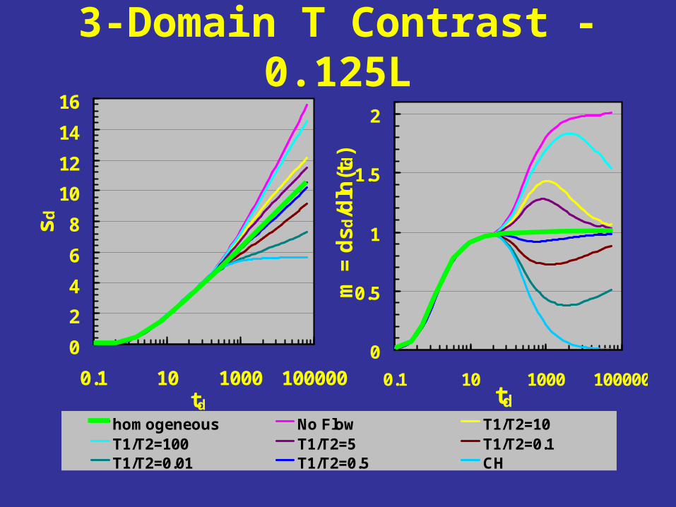
Strip Transmissivness & Conductance

• Hydraulic properties of the strip depend on strip conductivity and width

• Strip is a higher K than matrix

• Strip is a lower K than matrix

LK

wKT

a

ssd

a

sd K

L

w

KC

wKT ss

w

KC s

Strip Transmissivness & Conductance

010 52.1 98831min

min1

.CB.A

B

Cm

CmA

sdT

0.001

0.01

0.1

1

10

1 1.5 2

mmaxC

d

18.1 094.0

1maxmax2

BA

B

mm

Ad

C

0.1

1

10

100

1000

10000

0 0.5 1mmin

Tsd

Graphical EvaluationBoundary Type and Location

WellHigh T to Low TLow T to High T

0

5

10

15

20

0.1 10 1000 100000

td

s d

00.5

11.5

22.5

33.5

44.5

0.1 10 1000 100000

td

s d

Graphical EvaluationEstimate Aquifer Properties

0

2

4

6

8

10

12

14

16

0.001 0.01 0.1 1 10 100 1000

tdL

s d

to=0.029 S=0.017s=2.3 T=1

to=0.42 S=0.35s=4.1 T = 0.55

Graphical EvaluationEstimate Aquifer Properties

0

2

4

6

8

10

12

0.01 0.1 1 10 100 1000

tdL

s d

to = 2.7 S=0.136s = 4.1 T=0.55

TE=1SE=0.0179

TTLL=0.55=0.55SL=0.25

TE=1SE=0.0179

TTLL=0.55=0.55SL=0.136

TTLL=0.55=0.55SL=0.06

TTLL=0.55=0.55SL=0.27

TTLL=0.55=0.55SL=0.021

TTLL=0.55=0.55SL=0.068

TTLL=0.55=0.55SL=0.029

TTLL=0.55=0.55SL=0.021

L

L L

Graphical EvaluationEstimate Aquifer Properties

to=0.09 S = 0.054s = 2.3 T = 1

to=0.028 S = 0.017s = 2.3 T = 1

Determine Properties of Strip

• SSL analysis on the first line will give T and S of the area near the well.

• Take the derivative of time and determine the maximum or minimum slope.

• Using equations from curve fitting determine Tsd or Cd of the layer.

• Solve for Ts or C

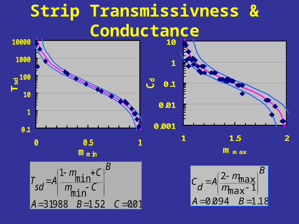
Field Case

K.G

. Fau

lt

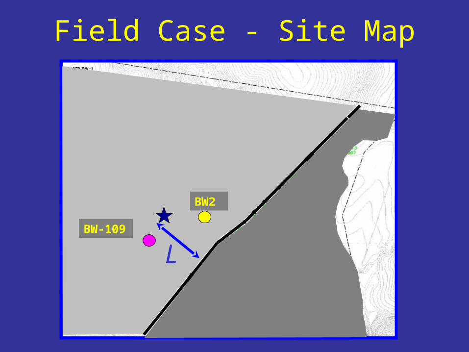
Field Case - Site Map

BW-109

BW2

L

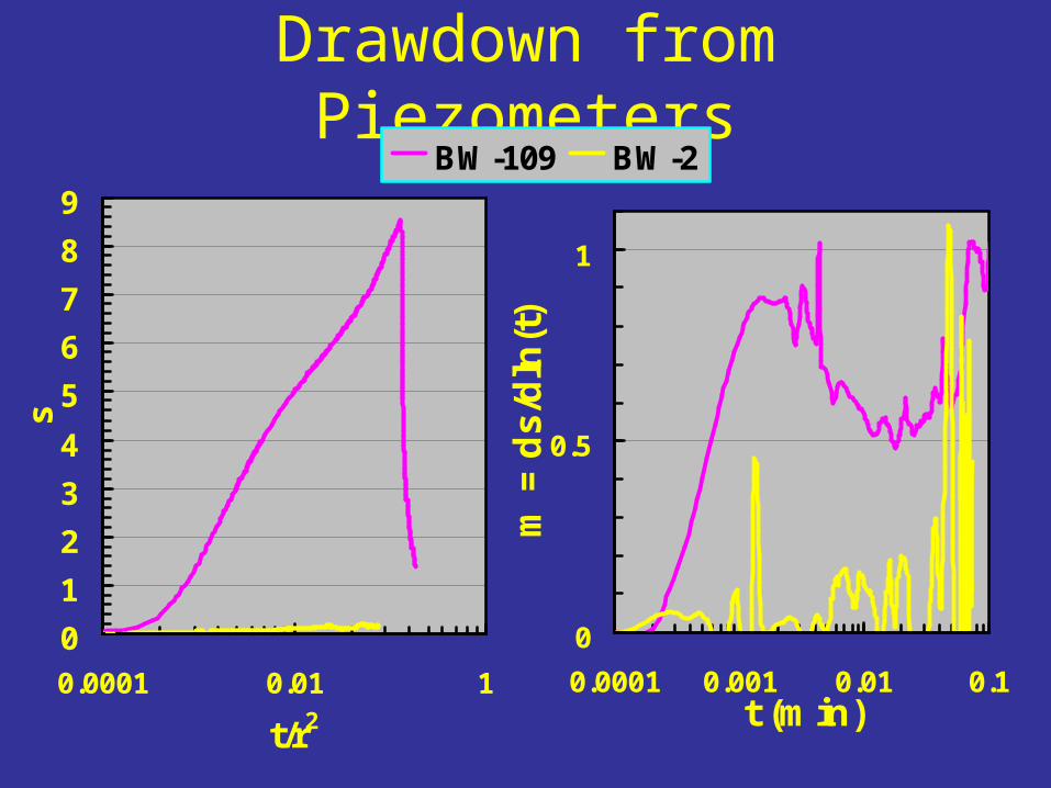
Drawdown from Piezometers

0

1

2

3

4

5

6

7

8

9

0.0001 0.01 1

t/r2

s

BW-109 BW-2

0

0.5

1

0.0001 0.001 0.01 0.1t (min)

m =

ds

/dln

(t)

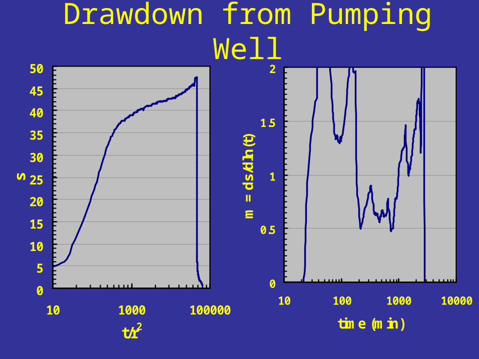
Drawdown from Pumping Well

0

5

10

15

20

25

30

35

40

45

50

10 1000 100000

t/r2

s

0

0.5

1

1.5

2

10 100 1000 10000

time (min)

m =

ds/

dln

(t)

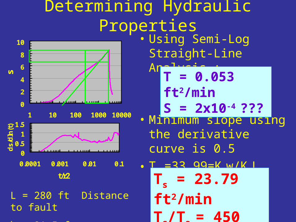
• Using Semi-Log Straight-Line Analysis :

• Minimum slope using the derivative curve is 0.5

• Tsd=33.99=Ksw/KaL

Determining Hydraulic Properties

0

2

4

6

8

10

1 10 100 1000 10000

t (min)

s

00.5

11.5

0.0001 0.001 0.01 0.1

t/r2

ds

/dln

(t)

L = 280 ft Distance to fault

b = 21.5 ft screened thickness

T = 0.053 ft2/minS = 2x10-4 ???

Ts = 23.79 ft2/minTs/Ta = 450

Conclusions 2-Domain Model

Semi-Log Straight-line Method• Piezometers r<0.3L gives T, S of local region.• Piezometers r>0.3L gives average T of both

regions.• Piezometers r>0.3L unable to predict S• Piezometers in neighboring region also give

average T of both regions.• Analyzing piezometers individually poor approach

to characterizing heterogeneities.

Conclusions 3-Domain Model• Drawdown for low conductivity vertical layer

controlled by conductance.

C=Ks/w • Drawdown for high conductivity vertical layer

controlled by strip transmissivness.

Ts=Ks*w• Feasible to determine properties of a vertical layer

from drawdown curves.• Drawdown curves non-unique. Require

geological assessment.