
WELL-POSEDNESS AND EXACT CONTROLLABILITY OF FOURTH ORDER...
32
Copyright © by SIAM. Unauthorized reproduction of this article is prohibited. SIAM J. CONTROL OPTIM. c 2014 Society for Industrial and Applied Mathematics Vol. 52, No. 1, pp. 365–396 WELL-POSEDNESS AND EXACT CONTROLLABILITY OF FOURTH ORDER SCHR ¨ ODINGER EQUATION WITH BOUNDARY CONTROL AND COLLOCATED OBSERVATION ∗ RUILI WEN † , SHUGEN CHAI ‡ , AND BAO-ZHU GUO § Abstract. In this paper, we study the well-posedness and exact controllability of a system described by a fourth order Schr¨odinger equation on a bounded domain of R n (n 2) with boundary control and collocated observation. The Neumann boundary control problem is first discussed. It is shown that the system is well-posed in the sense of D. Salamon. This implies the exponential stability of the closed-loop system under proportional output feedback control. The well-posedness result is then generalized to the Dirichlet boundary control problem. In particular, in order to conclude feedback stabilization from well-posedness, we discuss the exact controllability with the Dirichlet boundary control, which is similar to the Neumann boundary control case. In addition, we show that both systems are regular in the sense of G. Weiss and their feedthrough operators are zero. Key words. Schr¨ odinger equation, well-posedness, exact controllability, boundary control, boundary observation AMS subject classifications. 93C20, 93D25, 35B37 DOI. 10.1137/120902744 1. Introduction and main results. Well-posed systems belong to a wide class of linear infinite-dimensional systems which have been studied extensively in the last two decades; see, for instance, [5, 6, 7, 32, 35, 36, 37] and the references therein. This class of systems covers many partial differential equation control systems (PDEs) with actuators and sensors on isolated points, on subdomains, or on a part of the boundary of the spatial regions, with many properties parallel in many ways to those of finite-dimensional systems. Many PDEs have been verified to be well-posed. Some examples can be found in [1, 2, 4, 5, 6, 9, 10, 13, 14, 15, 33, 39]. In this paper, we study the well-posedness and exact controllability of a system described by a fourth order Schr¨ odinger equation with either Neumann or Dirichlet boundary control and associated collocated observation. Let Ω ⊂ R n (n 2) be an open bounded domain with a smooth C 3 -boundary ∂ Ω=Γ= Γ 0 ∪ Γ 1 . Assume that Γ 0 (int(Γ 0 ) = ∅) and Γ 1 are relatively open in ∂ Ω and Γ 0 ∩ Γ 1 = ∅, and let ν be the unit normal vector of ∂ Ω pointing to the exterior of Ω. The first objective of this paper is to establish the well-posedness of the system described by a fourth order Schr¨odinger equation with the Neumann control and collocated observation: ∗ Received by the editors December 17, 2012; accepted for publication (in revised form) November 20, 2013; published electronically February 4, 2014. This research was supported by the National Natural Science Foundation of China (11171195, 61273129), the Scholarship Council of Shanxi (2011- 015), the National Basic Research Program of China (2011CB808002), and the Deanship of Scientific Research (DSR), King Abdulaziz University (HiCi/1434/130-4). http://www.siam.org/journals/sicon/52-1/90274.html † School of Mathematical Sciences, Shanxi University, Taiyuan 030006, People’s Republic of China ([email protected]). ‡ Corresponding author. School of Mathematical Sciences, Shanxi University, Taiyuan 030006, People’s Republic of China ([email protected]). § Academy of Mathematics and System Sciences, Academia Sinica, Beijing 100190, People’s Republic of China, School of Computational and Applied Mathematics, University of the Witwa- tersrand, Wits 2050, Johannesburg, South Africa, and Depaartment of Mathematics, Faculty of Science, King Abdulaziz university, P.O. Box 80203, Jeddah 21589, Saudi Arabia ([email protected]). 365 Downloaded 02/05/14 to 124.16.148.9. Redistribution subject to SIAM license or copyright; see http://www.siam.org/journals/ojsa.php
Transcript of WELL-POSEDNESS AND EXACT CONTROLLABILITY OF FOURTH ORDER...

Copyright © by SIAM. Unauthorized reproduction of this article is prohibited.
SIAM J. CONTROL OPTIM. c© 2014 Society for Industrial and Applied MathematicsVol. 52, No. 1, pp. 365–396
WELL-POSEDNESS AND EXACT CONTROLLABILITY OF FOURTHORDER SCHRODINGER EQUATION WITH BOUNDARY
CONTROL AND COLLOCATED OBSERVATION∗
RUILI WEN† , SHUGEN CHAI‡ , AND BAO-ZHU GUO§
Abstract. In this paper, we study the well-posedness and exact controllability of a systemdescribed by a fourth order Schrodinger equation on a bounded domain of Rn(n � 2) with boundarycontrol and collocated observation. The Neumann boundary control problem is first discussed. It isshown that the system is well-posed in the sense of D. Salamon. This implies the exponential stabilityof the closed-loop system under proportional output feedback control. The well-posedness result isthen generalized to the Dirichlet boundary control problem. In particular, in order to concludefeedback stabilization from well-posedness, we discuss the exact controllability with the Dirichletboundary control, which is similar to the Neumann boundary control case. In addition, we showthat both systems are regular in the sense of G. Weiss and their feedthrough operators are zero.
Key words. Schrodinger equation, well-posedness, exact controllability, boundary control,boundary observation
AMS subject classifications. 93C20, 93D25, 35B37
DOI. 10.1137/120902744
1. Introduction and main results. Well-posed systems belong to a wide classof linear infinite-dimensional systems which have been studied extensively in the lasttwo decades; see, for instance, [5, 6, 7, 32, 35, 36, 37] and the references therein. Thisclass of systems covers many partial differential equation control systems (PDEs)with actuators and sensors on isolated points, on subdomains, or on a part of theboundary of the spatial regions, with many properties parallel in many ways to thoseof finite-dimensional systems. Many PDEs have been verified to be well-posed. Someexamples can be found in [1, 2, 4, 5, 6, 9, 10, 13, 14, 15, 33, 39]. In this paper, westudy the well-posedness and exact controllability of a system described by a fourthorder Schrodinger equation with either Neumann or Dirichlet boundary control andassociated collocated observation.
Let Ω ⊂ Rn(n � 2) be an open bounded domain with a smooth C3-boundary
∂Ω = Γ = Γ0∪Γ1. Assume that Γ0 (int(Γ0) �= ∅) and Γ1 are relatively open in ∂Ω andΓ0 ∩ Γ1 = ∅, and let ν be the unit normal vector of ∂Ω pointing to the exterior of Ω.
The first objective of this paper is to establish the well-posedness of the systemdescribed by a fourth order Schrodinger equation with the Neumann control andcollocated observation:
∗Received by the editors December 17, 2012; accepted for publication (in revised form) November20, 2013; published electronically February 4, 2014. This research was supported by the NationalNatural Science Foundation of China (11171195, 61273129), the Scholarship Council of Shanxi (2011-015), the National Basic Research Program of China (2011CB808002), and the Deanship of ScientificResearch (DSR), King Abdulaziz University (HiCi/1434/130-4).
http://www.siam.org/journals/sicon/52-1/90274.html†School of Mathematical Sciences, Shanxi University, Taiyuan 030006, People’s Republic of China
([email protected]).‡Corresponding author. School of Mathematical Sciences, Shanxi University, Taiyuan 030006,
People’s Republic of China ([email protected]).§Academy of Mathematics and System Sciences, Academia Sinica, Beijing 100190, People’s
Republic of China, School of Computational and Applied Mathematics, University of the Witwa-tersrand, Wits 2050, Johannesburg, South Africa, and Depaartment of Mathematics, Faculty ofScience, King Abdulaziz university, P.O. Box 80203, Jeddah 21589, Saudi Arabia ([email protected]).
365
Dow
nloa
ded
02/0
5/14
to 1
24.1
6.14
8.9.
Red
istr
ibut
ion
subj
ect t
o SI
AM
lice
nse
or c
opyr
ight
; see
http
://w
ww
.sia
m.o
rg/jo
urna
ls/o
jsa.
php

Copyright © by SIAM. Unauthorized reproduction of this article is prohibited.
366 RUILI WEN, SHUGEN CHAI, AND BAO-ZHU GUO
(1.1)
⎧⎪⎪⎪⎪⎪⎪⎪⎪⎪⎪⎪⎨⎪⎪⎪⎪⎪⎪⎪⎪⎪⎪⎪⎩
iwt(x, t) +�2w(x, t) = 0, x ∈ Ω, t > 0,
w(x, t) = 0, x ∈ ∂Ω, t � 0,
∂w(x, t)
∂ν= 0, x ∈ Γ1, t � 0,
∂w(x, t)
∂ν= u(x, t), x ∈ Γ0, t � 0,
y(x, t) = −iΔ((Δ2)−1w(x, t)), x ∈ Γ0, t � 0,
where u is the boundary control (input) and y is the boundary observation (output).The fourth order Schrodinger equation arises in quantum mechanics, nonlinear
optics, and plasma physics, and its general nonlinear form has been introduced in[19, 20] to take into account the role of small fourth order dispersion terms in thepropagation of intense laser beams in a bulk medium with Kerr nonlinearity. Theexistence and uniqueness of the solution have been studied intensively from the math-ematical perspective; see [16, 17, 29, 30] and the references therein. Here we considerthe control problem of the linear situation. Although there are many references on thecontrol problem for second order Schrodinger equations (see, e.g., [13, 22, 23]), theexact controllability of (1.1) has only recently been proved in [38].
Let H = H−2(Ω) and U = Y = L2(Γ0), where H−2(Ω) is the dual of the Sobolev
space H20 (Ω). The following theorem shows that system (1.1) is well-posed with the
state space H and the input and output space U = Y [15].Theorem 1.1. The system (1.1) is well-posed. More precisely, for any T > 0,
initial value w0 ∈ H, and control input u ∈ L2(0, T ;U), there exists a unique solutionw ∈ C(0, T ;H) to system (1.1) such that
(1.2) ‖w(·, T )‖2H + ‖y‖2L2(0,T ;U) � CT
[‖w0‖2H + ‖u‖2L2(0,T ;U)
],
where CT > 0 is a constant that depends only on Ω, Γ0, and T .Throughout the paper, we always use CT > 0 to represent a constant that depends
only on Ω, Γ0, and T . This constant may have different values in different contexts.The well-posedness claimed by Theorem 1.1 for the open loop control system (1.1)
is in the sense of D. Salamon, with the same input and output spaces U = Y and thestate space H . From this result and Theorems 6.7 and 6.8 of [11] on the first orderabstract system formulation (2.10) which are stated as Theorems 5.4 and 5.5 in theappendix of this paper (see also [24]), we know that system (1.1) is exactly controllablein some interval [0, T ], T > 0, if and only if its closed-loop system under the outputproportional feedback u = −ky, k > 0, is exponentially stable. This is different from[8], where the systems discussed usually do not satisfy condition (H2) for system(5.1) in the appendix of this paper. The following result is a direct consequence ofTheorem 1.1, exact controllability obtained in [38], and Theorem 5.5 in the appendix.
Corollary 1.2. Let x0 ∈ Rn and assume that Γ0 = {x ∈ ∂Ω| (x−x0)·ν(x) > 0}.
Then system (1.1) is exponentially stable under the output feedback u = −ky for anyk > 0.
According to Theorem 5.8 of [11] or Theorem 5.2 in the appendix, if the abstractsystem (2.10) introduced later is well-posed, it must be regular in the sense of G. Weisswith the zero feedthrough operator. The following result is hence a consequence ofTheorem 1.1.
Corollary 1.3. The system (1.1) is regular and the feedthrough operator iszero.
Dow
nloa
ded
02/0
5/14
to 1
24.1
6.14
8.9.
Red
istr
ibut
ion
subj
ect t
o SI
AM
lice
nse
or c
opyr
ight
; see
http
://w
ww
.sia
m.o
rg/jo
urna
ls/o
jsa.
php

Copyright © by SIAM. Unauthorized reproduction of this article is prohibited.
WELL-POSEDNESS AND EXACT CONTROLLABILITY 367
Remark 1.1. Perhaps we should mention a little bit about the solution of (1.1).Suppose that u ∈ H2
loc(0,∞;H3(Γ0)). Introduce the Dirichlet map [26, pp. 188–189]
γ ∈ L(Hs(Γ0), Hs+ 3
2 (Ω)) : (γu)(x, t) = φ(x, t) ∈ H2loc(0,∞;H4+ 1
2 (Ω)) if φ satisfies
(1.3)
⎧⎪⎪⎪⎪⎪⎪⎨⎪⎪⎪⎪⎪⎪⎩
Δ2φ(x, t) = 0, x ∈ Ω, t > 0,
φ|∂Ω =∂φ
∂ν
∣∣∣∣Γ1
= 0, t � 0,
∂φ
∂ν
∣∣∣∣Γ0
= u, t � 0.
It is obvious that φt ∈ H1loc(0,∞;H4+ 1
2 (Ω)). Let p(x, t) = w(x, t) − φ(x, t). Then psatisfies
(1.4)
⎧⎨⎩ipt(x, t) +�2p(x, t) = −iφt(x, t), x ∈ Ω, t > 0,
p(x, t) =∂p(x, t)
∂ν= 0, x ∈ ∂Ω, t � 0.
By the semigroup theory [28, Corollary 2.10], (1.4) admits a unique classical solution
p ∈ H1loc(0,∞;H4(Ω)) provided that p(·, 0) ∈ H4(Ω) satisfies p(x, 0) = ∂p(x,0)
∂ν = 0 forall x ∈ ∂Ω, which is the case if
(1.5)
⎧⎪⎨⎪⎩u ∈ H2
loc(0,∞;H3(Γ0)),
w(·, 0) ∈ H4(Ω), w(·, 0)|∂Ω =∂w(·, 0)∂ν
∣∣∣∣Γ1
= 0,∂w(·, 0)∂ν
∣∣∣∣Γ0
= u(·, 0).
For the classical solution, it is obvious that the output y in (1.1) makes sense. It isseen that the initial values and control input that satisfy condition (1.5) are dense inH and L2
loc(0,∞;U), respectively. Theorem 1.1 tells us that the classical solution canbe extended to the state space H for any w(·, 0) ∈ H and u ∈ L2
loc(0,∞;U) with thecontinuous dependence. A similar remark holds for system (1.6).
Next, we extend the result of Theorem 1.1 to the Dirichlet boundary control andcollocated observation of the following:
(1.6)
⎧⎪⎪⎪⎪⎪⎪⎪⎪⎪⎪⎪⎨⎪⎪⎪⎪⎪⎪⎪⎪⎪⎪⎪⎩
ivt(x, t) +�2v(x, t) = 0, x ∈ Ω, t > 0,
∂v(x, t)
∂ν= 0, x ∈ ∂Ω, t � 0,
v(x, t) = 0, x ∈ Γ1, t � 0,
v(x, t) = g(x, t), x ∈ Γ0, t � 0,
y(x, t) = i∂(Δ((Δ2)−3/2v(x, t)))
∂ν, x ∈ Γ0, t � 0,
where g is the boundary control (input) and y is the boundary observation (output).
Dow
nloa
ded
02/0
5/14
to 1
24.1
6.14
8.9.
Red
istr
ibut
ion
subj
ect t
o SI
AM
lice
nse
or c
opyr
ight
; see
http
://w
ww
.sia
m.o
rg/jo
urna
ls/o
jsa.
php

Copyright © by SIAM. Unauthorized reproduction of this article is prohibited.
368 RUILI WEN, SHUGEN CHAI, AND BAO-ZHU GUO
Let V = {ϕ ∈ H3(Ω)∣∣ ϕ|Γ = ∂ϕ
∂ν |Γ = 0}. The following theorem states that system(1.6) is well-posed in the state space V ′ which is the dual of space V with respect tothe pivot space L2(Ω) in the sense of Gelfand’s triple inclusions V ↪→ L2(Ω) ↪→ V ′,and the input and output space U = Y = L2(Γ0).
Theorem 1.4. The system (1.6) is well-posed. More precisely, for any T > 0,initial value v0 ∈ V ′, and control input g ∈ L2(0, T ;U), there exists a unique solutionv ∈ C(0, T ;V ′) to system (1.6) such that
(1.7) ‖v(·, T )‖2V ′ + ‖y‖2L2(0,T ;U) � CT
[‖v0‖2V ′ + ‖g‖2L2(0,T ;U)
].
In analogy to Corollary 1.3, we have the following consequence of Theorem 1.4.
Corollary 1.5. The system (1.6) is regular and the feedthrough operator iszero.
In order to generalize Corollary 1.2 to system (1.6), we need the exact controlla-bility of the open loop system (1.6), which is not available in the literature. In the lastpart of this paper, we show that under a certain geometric condition, system (1.6) isexactly controllable in time interval [0, T ], T > 0.
Theorem 1.6. Suppose that there exists a point x0 ∈ Rn such that
(1.8) (x− x0) · ν � σ > 0 on Γ.
Then for any v0 ∈ V ′, there exists a control g ∈ L2(0, T ;L2(Γ)) such that the uniquesolution v ∈ C(0, T ;V ′) of (1.6) satisfies v(T ) = 0.
Now we state system (1.6) a result, which is parallel to Corollary 1.2 for system(1.1). The result is a consequence of Theorems 1.4 and 1.6.
Corollary 1.7. Let x0 ∈ Rn and (1.8) hold. Then system (1.6) is exponentially
stable under the output feedback g = −ky for any k > 0.The rest of the paper is organized as follows. In section 2, we formulate system
(1.1) into a collocated abstract first order system and give the proof of Theorem 1.1.The proof of Theorem 1.4 is presented in section 3. Section 4 is devoted to the proofof Theorem 1.6.
2. Proof of Theorem 1.1. In this section, we first cast the system (1.1) into anabstract framework of a first order collocated system with state space H and controland output spaces U = Y .
Let A be the positive self-adjoint operator in H induced by the sesquilinear forma(·, ·) given by
(2.1) 〈Aϕ,ψ〉H−2(Ω),H20 (Ω) = a(ϕ, ψ) =
∫Ω
Δϕ(x)Δψ(x)dx ∀ ϕ, ψ ∈ H20 (Ω).
According to the Lax–Milgram theorem, A is a canonical isomorphism from D(A) =H2
0 (Ω) onto H . If we introduce Δ2 : H4(Ω)∩H20 (Ω) → L2(Ω), then it is easy to show
that Af = Δ2f for f ∈ H4(Ω) ∩ H20 (Ω) and that A−1ϕ = (Δ2)−1ϕ for ϕ ∈ L2(Ω).
Hence A is an extension of the usual biharmornic operator to the space H20 (Ω).
It is well known that D(A1/2) = L2(Ω) and A1/2 is a canonical isomorphism from
L2(Ω) onto H (see, e.g., [14]). Let the Dirichlet map γ ∈ L(L2(Γ0), H32 (Ω)): γu = φ
be defined by (1.3). Using the Dirichlet map, we can rewrite (1.1) as
(2.2) iw +A(w − γu) = 0.
Dow
nloa
ded
02/0
5/14
to 1
24.1
6.14
8.9.
Red
istr
ibut
ion
subj
ect t
o SI
AM
lice
nse
or c
opyr
ight
; see
http
://w
ww
.sia
m.o
rg/jo
urna
ls/o
jsa.
php

Copyright © by SIAM. Unauthorized reproduction of this article is prohibited.
WELL-POSEDNESS AND EXACT CONTROLLABILITY 369
Clearly D(A) is dense in H , and so is D(A1/2) in H . We identify H with its dual H ′.Then the following Gelfand-triple of continuous and dense inclusions hold:
(2.3) D(A1/2) ↪→ H = H ′ ↪→ D(A1/2)′.
An extension A ∈ L(D(A1/2), D(A1/2)′) of A is defined as follows:
(2.4) 〈Aϕ, ψ〉D(A1/2)′,D(A1/2) = 〈A1/2ϕ,A1/2ψ〉H ∀ ϕ, ψ ∈ D(A1/2).
Hence (2.2) can be written in D(A1/2)′ as
(2.5) w = iAw +Bu,
where B ∈ L(U,D(A1/2)′) is given by
(2.6) Bu = −iAγu ∀ u ∈ L2(Γ0).
Define B∗ ∈ L(D(A1/2), U) by
(2.7) 〈B∗f, u〉U = 〈f,Bu〉D(A1/2),D(A1/2)′ ∀ f ∈ D(A1/2), u ∈ U.
Then for any f ∈ D(A1/2) and u ∈ C∞0 (Γ0), we have
〈f,Bu〉D(A1/2),D(A1/2)′ = 〈Af, A−1Bu〉D(A1/2)′,D(A1/2)(2.8)
= 〈A1/2f,A1/2A−1Bu〉H= 〈A−1A1/2f,A−1A1/2A−1Bu〉H2
0 (Ω)
= 〈A−1/2f,A−1/2(−iγu)〉H20 (Ω) = 〈f,−iγu〉L2(Ω)
= 〈AA−1f,−iγu〉L2(Ω) = 〈−iΔ((Δ2)−1f), u〉U .
Since C∞0 (Γ0) is dense in L2(Γ0), we obtain
(2.9) B∗f = −iΔ((Δ2)−1f) ∀ f ∈ D(A1/2) = L2(Ω).
System (1.1) is thus formulated as a first order abstract collocated system in the statespace H and control and output space U = Y :
(2.10)
{w = iAω +Bu,
y = B∗w,
where A, B, and B∗ are defined by (2.4), (2.6), and (2.7), respectively.In order to prove Theorem 1.1, we need the following lemma, which comes from
Theorem 4.9 of [11]. (See also [25] and Theorem 5.1 in the appendix.)Lemma 2.1. If there exist constants T > 0, CT > 0 such that the input and
output of system (1.1) satisfy∫ T
0
‖y(t)‖2Udt � CT
∫ T
0
‖u(t)‖2Udt
with w(·, 0) ≡ 0, then system (1.1) is well-posed.
Dow
nloa
ded
02/0
5/14
to 1
24.1
6.14
8.9.
Red
istr
ibut
ion
subj
ect t
o SI
AM
lice
nse
or c
opyr
ight
; see
http
://w
ww
.sia
m.o
rg/jo
urna
ls/o
jsa.
php

Copyright © by SIAM. Unauthorized reproduction of this article is prohibited.
370 RUILI WEN, SHUGEN CHAI, AND BAO-ZHU GUO
Proof of Theorem 1.1. By Remark 1.1, it suffices to prove (1.2) for those w(·, 0)and u that satisfy condition (1.5) and then conclude for general w(·, 0) ∈ H andu ∈ L2(0,∞;U) by the density argument. Let z = A−1w ∈ H1
loc(0,∞;H4(Ω)). Thenz satisfies
(2.11)
⎧⎪⎪⎪⎨⎪⎪⎪⎩zt(x, t) − iΔ2z(x, t) = −i(γu(·, t))(x, t), (x, t) ∈ Ω× (0, T ],
z(x, 0) = z0(x), x ∈ Ω,
z(x, t) =∂z(x, t)
∂ν= 0, (x, t) ∈ ∂Ω× [0, T ],
and the output of system (1.1) is changed into the following form:
y(x, t) = B∗w(x, t) = B∗AA−1w(x, t)(2.12)
= B∗Az(x, t) = −i�z(x, t), x ∈ Γ0, t > 0.
By Lemma 2.1, in order to prove Theorem 1.1, we need only prove that there existsa constant CT > 0 satisfying
(2.13)
∫ T
0
∫Γ0
|y(x, t)|2dΓdt � CT
∫ T
0
∫Γ0
|u(x, t)|2dΓdt
for system (2.11) with the output (2.12) and initial value z0 = 0.Since ∂Ω is of class C3, it follows from Lemma 2.1 of [21, p. 18] that there exists
a vector field h = (h1, h2, . . . , hn) : Ω → Rn of class C2 such that h(x) = ν(x) on ∂Ω
and |h| � 1, where | · | denotes the Euclidean norm of Rn.Multiply both sides of the first equation of (2.11) by h·�z and perform integration
over Ω× (0, T ] to obtain
(2.14)
∫ T
0
∫Ω
zth · ∇zdxdt− i
∫ T
0
∫Ω
Δ2zh · ∇zdxdt = −i
∫ T
0
∫Ω
(γu)h · ∇zdxdt.
Now computing the first term on the left-hand side (LHS) of (2.14) by integration byparts, we obtain∫ T
0
∫Ω
zth · ∇zdxdt =∫Ω
zh · ∇zdx∣∣∣∣T0
−∫ T
0
∫Ω
zh · ∇ztdxdt
=
(∫Ω
div(h|z|2)dx−∫Ω
zh · ∇zdx−∫Ω
|z|2div(h)dx) ∣∣∣∣T
0
−(∫ T
0
∫Ω
div(zzth)dxdt −∫ T
0
∫Ω
zth · ∇zdxdt−∫ T
0
∫Ω
zztdiv(h)dxdt
)and hence
2iIm
∫ T
0
∫Ω
zth · ∇zdxdt(2.15)
=
∫ T
0
∫Ω
zztdiv(h)dxdt −(∫
Ω
zh · ∇zdx+
∫Ω
|z|2div(h)dx) ∣∣∣∣T
0
= i
∫ T
0
∫Ω
zγudiv(h)dxdt − i
∫ T
0
∫Ω
zΔ2zdiv(h)dxdt
−(∫
Ω
zh · ∇zdx+∫Ω
|z|2div(h)dx) ∣∣∣∣T
0
.
Dow
nloa
ded
02/0
5/14
to 1
24.1
6.14
8.9.
Red
istr
ibut
ion
subj
ect t
o SI
AM
lice
nse
or c
opyr
ight
; see
http
://w
ww
.sia
m.o
rg/jo
urna
ls/o
jsa.
php
Copyright © by SIAM. Unauthorized reproduction of this article is prohibited.
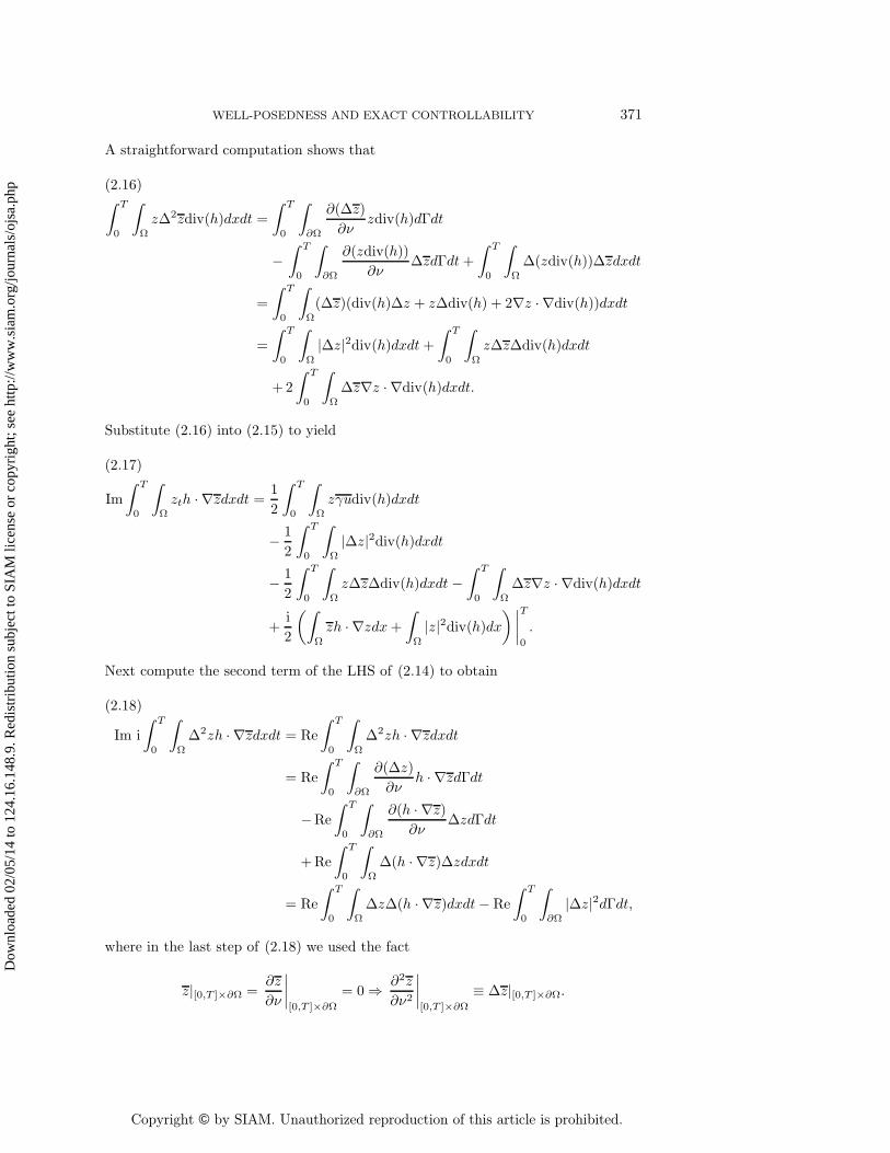
WELL-POSEDNESS AND EXACT CONTROLLABILITY 371
A straightforward computation shows that
(2.16)∫ T
0
∫Ω
zΔ2zdiv(h)dxdt =
∫ T
0
∫∂Ω
∂(Δz)
∂νzdiv(h)dΓdt
−∫ T
0
∫∂Ω
∂(zdiv(h))
∂νΔzdΓdt+
∫ T
0
∫Ω
Δ(zdiv(h))Δzdxdt
=
∫ T
0
∫Ω
(Δz)(div(h)Δz + zΔdiv(h) + 2∇z · ∇div(h))dxdt
=
∫ T
0
∫Ω
|Δz|2div(h)dxdt+∫ T
0
∫Ω
zΔzΔdiv(h)dxdt
+2
∫ T
0
∫Ω
Δz∇z · ∇div(h)dxdt.
Substitute (2.16) into (2.15) to yield
(2.17)
Im
∫ T
0
∫Ω
zth · ∇zdxdt = 1
2
∫ T
0
∫Ω
zγudiv(h)dxdt
− 1
2
∫ T
0
∫Ω
|Δz|2div(h)dxdt
− 1
2
∫ T
0
∫Ω
zΔzΔdiv(h)dxdt −∫ T
0
∫Ω
Δz∇z · ∇div(h)dxdt
+i
2
(∫Ω
zh · ∇zdx+
∫Ω
|z|2div(h)dx) ∣∣∣∣T
0
.
Next compute the second term of the LHS of (2.14) to obtain
Im i
∫ T
0
∫Ω
Δ2zh · ∇zdxdt = Re
∫ T
0
∫Ω
Δ2zh · ∇zdxdt(2.18)
= Re
∫ T
0
∫∂Ω
∂(Δz)
∂νh · ∇zdΓdt
−Re
∫ T
0
∫∂Ω
∂(h · ∇z)∂ν
ΔzdΓdt
+Re
∫ T
0
∫Ω
Δ(h · ∇z)Δzdxdt
= Re
∫ T
0
∫Ω
ΔzΔ(h · ∇z)dxdt− Re
∫ T
0
∫∂Ω
|Δz|2dΓdt,
where in the last step of (2.18) we used the fact
z|[0,T ]×∂Ω =∂z
∂ν
∣∣∣∣[0,T ]×∂Ω
= 0 ⇒ ∂2z
∂ν2
∣∣∣∣[0,T ]×∂Ω
≡ Δz|[0,T ]×∂Ω.
Dow
nloa
ded
02/0
5/14
to 1
24.1
6.14
8.9.
Red
istr
ibut
ion
subj
ect t
o SI
AM
lice
nse
or c
opyr
ight
; see
http
://w
ww
.sia
m.o
rg/jo
urna
ls/o
jsa.
php

Copyright © by SIAM. Unauthorized reproduction of this article is prohibited.
372 RUILI WEN, SHUGEN CHAI, AND BAO-ZHU GUO
Another straightforward computation shows that
ReΔzΔ(h · ∇z) = Re
⎡⎣Δz⎛⎝ n∑
i,j=1
∂2hi∂x2j
∂z
∂xi
⎞⎠⎤⎦(2.19)
+Re
⎡⎣Δz⎛⎝2 n∑
i,j=1
∂hi∂xj
∂2z
∂xi∂xj
⎞⎠⎤⎦+1
2div
(|Δz|2h)− 1
2|Δz|2div(h).
Substitute (2.19) into (2.18) to give
Im i
∫ T
0
∫Ω
Δ2zh · ∇zdxdt = Re
∫ T
0
∫Ω
Δz
⎛⎝ n∑i,j=1
∂2hi∂x2j
∂z
∂xi
⎞⎠ dxdt
(2.20)
+Re
∫ T
0
∫Ω
⎡⎣Δz⎛⎝2
n∑i,j=1
∂hi∂xj
∂2z
∂xi∂xj
⎞⎠⎤⎦ dxdt− 1
2
∫ T
0
∫Ω
|Δz|2div(h)dxdt − 1
2
∫ T
0
∫∂Ω
|Δz|2dΓdt.
Let H = Dh, that is,
H =
⎛⎜⎝∂h1
∂x1,· · · ∂h1
∂xn
.... . .
...∂hn
∂x1,· · · ∂hn
∂xn
⎞⎟⎠ .
Then we have the following equality:
(2.21) div[(H +HT ) · ∇z] =n∑
i,j=1
∂2hi∂x2j
∂z
∂xi+ 2
n∑i,j=1
∂hi∂xj
∂2z
∂xi∂xj+
n∑i,j=1
∂z
∂xj
∂2hi∂xi∂xj
.
Combining (2.14), (2.17), (2.20), and (2.21), we get
1
2
∫ T
0
∫∂Ω
|Δz|2dΓdt(2.22)
=Re
∫ T
0
∫Ω
Δzdiv[(H +HT ) · ∇z] dxdt
+1
2Re
∫ T
0
∫Ω
zΔzΔdiv(h)dxdt (� R1)
− 1
2Re
∫ T
0
∫Ω
z(γu)div(h)dxdt− Re
∫ T
0
∫Ω
(γu)h · ∇zdxdt (� R2)
+1
2Im
(∫Ω
zh · ∇zdx+∫Ω
|z|2div(h)dx) ∣∣∣∣T
0
(� b0,T ).
Now we estimate R1, R2, b0,T in the following three steps.
Dow
nloa
ded
02/0
5/14
to 1
24.1
6.14
8.9.
Red
istr
ibut
ion
subj
ect t
o SI
AM
lice
nse
or c
opyr
ight
; see
http
://w
ww
.sia
m.o
rg/jo
urna
ls/o
jsa.
php

Copyright © by SIAM. Unauthorized reproduction of this article is prohibited.
WELL-POSEDNESS AND EXACT CONTROLLABILITY 373
Step 1: Estimation of R1. Let γu = 0 in the first identity of (2.11) and notethat z = A−1w ∈ H2
0 (Ω). It is known that (2.11) associates with a C0-group solutionin H2
0 (Ω), that is, for any z0 ∈ H20 (Ω), there exists a unique solution z ∈ H2
0 (Ω) to(2.11), which depends continuously on z0. This fact together with (2.22) implies that
1
2
∫ T
0
∫∂Ω
|Δz|2dΓdt � CT ‖z0‖2H20 (Ω).
Hence the operator B∗ is admissible, and so is B (see, e.g., [5] and Theorem 4.4.3 of[34]). In other words,
(2.23) u→ w is continous from L2(0, T ;L2(Γ0)) to C(0, T ;H−2(Ω)).
Moreover,
(2.24) z = A−1w ∈ C(0, T ;H20 (Ω)) depends continuously on u ∈ L2(0, T ;L2(Γ0))
because of A−1 ∈ L(H−2(Ω), H20 (Ω)). Therefore
(2.25) R1 � CT ‖u‖2L2(0,T ;L2(Γ0))∀ u ∈ L2(0, T ;L2(Γ0)).
In what follows, we assume that w(x, 0) ≡ 0.Step 2: Estimation of R2. To begin with, let us consider the first term of R2:
− 1
2Re
∫ T
0
∫Ω
z(γu)div(h)dxdt = −1
2Re
∫ T
0
∫Ω
div(z(γu)h)dxdt(2.26)
+1
2Re
∫ T
0
∫Ω
zh · ∇(γu)dxdt +1
2Re
∫ T
0
∫Ω
(γu)h · ∇zdxdt
=1
2Re
∫ T
0
∫Ω
zh · ∇(γu)dxdt +1
2Re
∫ T
0
∫Ω
(γu)h · ∇zdxdt.
Since (γu) ∈ L2(0, T ;H32 (Ω)), it follows that ∇(γu) ∈ L2(0, T ;H
12 (Ω)). So both terms
in the last row of (2.26) depend continuously on u ∈ L2(0, T ;L2(Γ0)). From thesefacts and (2.24), we obtain
(2.27) −1
2Re
∫ T
0
∫Ω
z(γu)div(h)dxdt � CT ‖u‖2L2(0,T ;L2(Γ0)).
Similarly,
(2.28) −Re
∫ T
0
∫Ω
(γu)h · ∇zdxdt � CT ‖u‖2L2(0,T ;L2(Γ0)).
From (2.27) and (2.28), we have
(2.29) R2 � CT ‖u‖2L2(0,T ;L2(Γ0)).
This is Step 2.Step 3: Estimation of b0,T . Since w ∈ C(0, T ;H−2(Ω)) depends continuously
on u ∈ L2(0, T ;L2(Γ0)) and A−1 ∈ L(H−2(Ω), H2
0 (Ω)), we have
(2.30)
⎧⎪⎪⎨⎪⎪⎩z(·, 0) = A−1w(·, 0) = 0,
z(·, T ) = A−1w(·, T ) ∈ H20 (Ω) depends continuously on
u ∈ L2(0, T ;L2(Γ0)).
Dow
nloa
ded
02/0
5/14
to 1
24.1
6.14
8.9.
Red
istr
ibut
ion
subj
ect t
o SI
AM
lice
nse
or c
opyr
ight
; see
http
://w
ww
.sia
m.o
rg/jo
urna
ls/o
jsa.
php

Copyright © by SIAM. Unauthorized reproduction of this article is prohibited.
374 RUILI WEN, SHUGEN CHAI, AND BAO-ZHU GUO
From (2.24) and (2.30), we obtain
(2.31) b0,T � CT ‖u‖2L2(0,T ;L2(Γ0)).
This is Step 3. Equation (2.13) is then obtained by combining (2.22), (2.25), (2.29),(2.31), and (2.12).
3. Proof of Theorem 1.4. Again we formulate system (1.6) as an abstractfirst order collocated system in the state space H1 = V ′ and control and output spaceU = Y = L2(Γ0). Define the operator A by
(3.1) A f = −Δf ∀ f ∈ D(A ) = H2(Ω) ∩H10 (Ω).
Let A1 be the positive self-adjoint operator in L2(Ω) defined by
(3.2)
{A1ϕ = Δ2ϕ,
D(A1) = H4(Ω) ∩H20 (Ω).
It can be easily shown that A1/21 = A (see, e.g., [14]). Moreover,
(3.3) V � D(A3/41 ) =
{ϕ ∈ H3(Ω)|ϕ|Γ =
∂ϕ
∂ν
∣∣∣∣Γ
= 0
}.
Define an extension operator A of A1 to the space V ′ by
(3.4) 〈Aϕ, ψ〉V ′ = 〈A1/21 ϕ,A
1/21 ψ〉V ′ ∀ ϕ, ψ ∈ V.
We claim that A is a positive self-adjoint operator in V ′. In fact,
〈Aϕ, ϕ〉V ′ = 〈A1/21 ϕ,A
1/21 ϕ〉V ′ = 〈A−1/4
1 ϕ,A−1/41 ϕ〉L2(Ω)(3.5)
� C‖ϕ‖2L2(Ω) � C′‖A−3/41 ϕ‖2L2(Ω) = C′‖ϕ‖2V ′ ∀ ϕ ∈ V,
where C,C′ > 0 are constants. Identifying H1 with its dual H ′1, we have the following
Gelfand triple inclusions:
(3.6) D(A1/2) ↪→ H1 = H ′1 ↪→ D(A1/2)′.
Define an extension A1 ∈ L(D(A1/2), D(A1/2)′) of A:
(3.7) 〈A1ϕ, ψ〉D(A1/2)′,D(A1/2) = 〈A1/2ϕ,A1/2ψ〉V ′ ∀ ϕ, ψ ∈ D(A1/2).
Let G be the map: G ∈ L(L2(Γ0), H1/2(Ω)) [26, pp. 188–189] so that Gg = φ if
(3.8)
⎧⎪⎨⎪⎩Δ2φ(x) = 0, x ∈ Ω,
∂φ(x)
∂ν
∣∣∣∣Γ
= 0, φ(x)∣∣Γ1
= 0, φ(x)∣∣Γ0
= g.
In terms of A1 and G, system (1.6) can be written in D(A1/2)′ as
(3.9) v = iA1v +B1g,
Dow
nloa
ded
02/0
5/14
to 1
24.1
6.14
8.9.
Red
istr
ibut
ion
subj
ect t
o SI
AM
lice
nse
or c
opyr
ight
; see
http
://w
ww
.sia
m.o
rg/jo
urna
ls/o
jsa.
php

Copyright © by SIAM. Unauthorized reproduction of this article is prohibited.
WELL-POSEDNESS AND EXACT CONTROLLABILITY 375
where B1 ∈ L(U,D(A1/2)′) is given by
(3.10) B1g = −iA1Gg ∀ g ∈ L2(Γ0).
Define B∗1 ∈ L(D(A1/2), U) by
(3.11) 〈g,B∗1f〉U = 〈B1g, f〉D(A1/2)′,D(A1/2) ∀ f ∈ D(A1/2) = H1
0 (Ω), g ∈ U.
Then for any f ∈ D(A1/2) and g ∈ C∞0 (Γ0), we have
〈B1g, f〉D(A1/2)′,D(A1/2) = 〈−iA1Gg, f〉D(A1/2)′,D(A1/2)
(3.12)
= 〈−iA1/2Gg,A1/2f〉V ′ = 〈−iAGg,A3/2(A−3/2f)〉V ′
= 〈−iA−3/41 A1Gg,A
−3/41 A
3/21 (A
−3/21 f)〉L2(Ω)
= 〈−iGg,Δ2(A−3/21 f)〉L2(Ω) =
⟨g, i
∂(Δ((Δ2)−3/2f))
∂ν
⟩U
.
Since C∞0 (Γ0) is dense in L2(Γ0), we have
(3.13) B∗1f = i
∂(Δ((Δ2)−3/2f))
∂ν
∣∣∣∣Γ0
∀ f ∈ D(A1/2) = H10 (Ω).
Hence, we can formulate the open-loop system (1.6) as a first order abstract formin V ′:
(3.14)
{v = iA1v +B1g,y = B∗
1v,
where A1, B1, B∗1 are defined by (3.7), (3.10), and (3.11), respectively.
Proof of Theorem 1.4. By Lemma 2.1, Theorem 1.4 is equivalent to the statementthat the solution to system (1.6) with zero initial data satisfies
(3.15) ‖y‖2L2(0,T ;L2(Γ0))� CT ‖g‖2L2(0,T ;L2(Γ0))
∀ g ∈ L2(0, T ;L2(Γ0)).
As is indicated in the beginning of the proof of Theorem 1.1, we may suppose thatg is smooth (see Remark 1.1), that is, dense in L2
loc(0,∞;U), and then concludeto general g ∈ L2
loc(0,∞;U) by the density argument. Make a transformation z =
A−3/21 v ∈ H1(0, T ;H4(Ω)). Instead of (1.6), we consider the following system in V :
(3.16)
⎧⎪⎪⎪⎪⎪⎪⎪⎪⎨⎪⎪⎪⎪⎪⎪⎪⎪⎩
zt(x, t) = iΔ2z(x, t)− i(A−1/21 Gg(·, t))(x, t), (x, t) ∈ Ω× (0, T ],
z(x, 0) = 0, x ∈ Ω,
z(x, t) =∂z(x, t)
∂ν= 0, (x, t) ∈ ∂Ω× [0, T ],
y(x, t) = i∂(Δz(x, t))
∂ν, (x, t) ∈ ∂Ω× [0, T ].
So Theorem 1.4 holds true if and only if for some (and hence for all) T > 0, there existsa CT > 0 such that the solution to (3.16) satisfies (consider smooth g if necessary;see Remark 1.1)
(3.17)
∫ T
0
∫Γ0
∣∣∣∣∂(Δz(x, t))∂ν
∣∣∣∣2 dΓdt � CT
∫ T
0
∫Γ0
|g(x, t)|2 dΓdt.
Dow
nloa
ded
02/0
5/14
to 1
24.1
6.14
8.9.
Red
istr
ibut
ion
subj
ect t
o SI
AM
lice
nse
or c
opyr
ight
; see
http
://w
ww
.sia
m.o
rg/jo
urna
ls/o
jsa.
php

Copyright © by SIAM. Unauthorized reproduction of this article is prohibited.
376 RUILI WEN, SHUGEN CHAI, AND BAO-ZHU GUO
Let p(x, t) = (A−1/21 Gg(·, t))(x, t). Then by the definitions of A1 and G, we have
(3.18)
∫ T
0
‖p(x, t)‖2L2(Ω)dt � CT
∫ T
0
‖g(·, t)‖2L2(Γ0)dt.
Now, let q(x) ∈ C2(Ω) be an arbitrary smooth vector field and multiply both sidesof the first equation of (3.16) by q · ∇(Δz) and perform integration over Ω× (0, T ] toobtain
(3.19)∫ T
0
∫Ω
ztq · ∇(Δz)dxdt − i
∫ T
0
∫Ω
Δ2zq · ∇(Δz)dxdt + i
∫ T
0
∫Ω
pq · ∇(Δz)dxdt = 0.
Computing the second term on the LHS of (3.19) gives
i
∫ T
0
∫Ω
Δ2zq · ∇(Δz)dxdt = i
∫ T
0
∫∂Ω
∂(Δz)
∂νq · ∇(Δz)dΓdt(3.20)
− i
∫ T
0
∫Ω
∇(Δz) · ∇(q · ∇(Δz))dxdt.
A direct computation shows that
Re [∇(Δz) · ∇(q · ∇(Δz))] = Re
⎡⎣ n∑i,j=1
∂qj∂xi
∂(Δz)
∂xi
∂(Δz)
∂xj
⎤⎦(3.21)
+1
2div
(|∇(Δz)|2q)− 1
2|∇(Δz)|2div(q).
Substitute (3.21) into (3.20) to give
Im i
∫ T
0
∫Ω
Δ2zq · ∇(Δz)dxdt = Re
∫ T
0
∫∂Ω
∂(Δz)
∂νq · ∇(Δz)dΓdt(3.22)
−Re
∫ T
0
∫Ω
n∑i,j=1
∂qj∂xi
∂(Δz)
∂xi
∂(Δz)
∂xjdxdt
− 1
2
∫ T
0
∫∂Ω
∣∣∇(Δz)∣∣2q · νdΓdt
+1
2
∫ T
0
∫Ω
∣∣∇(Δz)∣∣2div(q)dxdt.
Next, we compute the first term on the LHS of (3.19). By virtue of the divergenceformula, we have
(3.23)
div(ztΔzq) = ztΔzdiv(q) + ztq · ∇(Δz) + Δzq · ∇zt= (iΔ2z − ip)Δzdiv(q) + ztq · ∇(Δz) +
d
dt(Δzq · ∇z)−Δztq · ∇z,
Dow
nloa
ded
02/0
5/14
to 1
24.1
6.14
8.9.
Red
istr
ibut
ion
subj
ect t
o SI
AM
lice
nse
or c
opyr
ight
; see
http
://w
ww
.sia
m.o
rg/jo
urna
ls/o
jsa.
php

Copyright © by SIAM. Unauthorized reproduction of this article is prohibited.
WELL-POSEDNESS AND EXACT CONTROLLABILITY 377
in which ∫ T
0
∫Ω
Δztq · ∇zdxdt =∫ T
0
∫∂Ω
∂zt∂ν
q · ∇zdΓdt+∫ T
0
∫Ω
ztΔq · ∇zdxdt(3.24)
+
∫ T
0
∫Ω
ztq · ∇(Δz)dxdt
+2
∫ T
0
∫Ω
zt
n∑i,j=1
∂qi∂xj
∂2z
∂xi∂xjdxdt.
Notice that in deriving (3.24), we used the fact
Δ(q · ∇z) = Δq · ∇z + q · ∇(Δz) + 2
n∑i,j=1
∂qi∂xj
∂2z
∂xi∂xj,(3.25)
Δq = (Δq1,Δq2, . . . ,Δqn).
Integrating the equality (3.23) over Ω× (0, T ] by taking (3.24) into account yields
Im
∫ T
0
∫Ω
ztq · ∇(Δz)dxdt
(3.26)
=1
2
∫ T
0
∫Ω
pΔzdiv(q)dxdt
− 1
2
∫ T
0
∫Ω
Δ2zΔzdiv(q)dxdt +i
2
∫Ω
Δzq · ∇zdx∣∣T0
− i
2
∫ T
0
∫Ω
ztΔq · ∇zdxdt− i
∫ T
0
∫Ω
zt
n∑i,j=1
∂qi∂xj
∂2z
∂xi∂xjdxdt
− i
2
∫ T
0
∫∂Ω
∂zt∂ν
q · ∇zdΓdt
=1
2
∫ T
0
∫Ω
pΔzdiv(q)dxdt − 1
2
∫ T
0
∫Ω
Δ2zΔzdiv(q)dxdt +i
2
∫Ω
Δzq · ∇zdx∣∣T0
− 1
2
∫ T
0
∫Ω
(Δ2z − p)Δq · ∇zdxdt−∫ T
0
∫Ω
(Δ2z − p)
n∑i,j=1
∂qi∂xj
∂2z
∂xi∂xjdxdt
− i
2
∫ T
0
∫∂Ω
∂zt∂ν
q · ∇zdΓdt
=1
2
∫ T
0
∫Ω
pΔzdiv(q)dxdt − 1
2
∫ T
0
∫∂Ω
∂(Δz)
∂νΔzdiv(q)dΓdt
+1
2
∫ T
0
∫Ω
|∇(Δz)|2div(q)dxdt
+1
2
∫ T
0
∫Ω
Δz∇(Δz) · ∇(div(q))dxdt +i
2
∫Ω
Δzq · ∇zdx∣∣T0
− 1
2
∫ T
0
∫∂Ω
∂(Δz)
∂νΔq · ∇zdΓdt
Dow
nloa
ded
02/0
5/14
to 1
24.1
6.14
8.9.
Red
istr
ibut
ion
subj
ect t
o SI
AM
lice
nse
or c
opyr
ight
; see
http
://w
ww
.sia
m.o
rg/jo
urna
ls/o
jsa.
php

Copyright © by SIAM. Unauthorized reproduction of this article is prohibited.
378 RUILI WEN, SHUGEN CHAI, AND BAO-ZHU GUO
+1
2
∫ T
0
∫Ω
∇(Δz) · ∇(Δq · ∇z)dxdt+ 1
2
∫ T
0
∫Ω
pΔq · ∇zdxdt
−∫ T
0
∫∂Ω
∂(Δz)
∂ν
n∑i,j=1
∂qi∂xj
∂2z
∂xi∂xjdΓdt
+
∫ T
0
∫Ω
∇(Δz) · ∇⎛⎝ n∑
i,j=1
∂qi∂xj
∂2z
∂xi∂xj
⎞⎠ dxdt
+
∫ T
0
∫Ω
p
n∑i,j=1
∂qi∂xj
∂2z
∂xi∂xjdxdt − i
2
∫ T
0
∫∂Ω
∂zt∂ν
q · ∇zdΓdt.
Set q = h, which is the same as that in the proof of Theorem 1.1, h(x) = ν(x) on ∂Ω,and |h| � 1, in (3.22) and (3.26) to get, respectively, that
Im i
∫ T
0
∫Ω
Δ2zh · ∇(Δz)dxdt
(3.27)
=1
2
∫ T
0
∫∂Ω
∣∣∣∣∂(Δz)∂ν
∣∣∣∣2 dΓdt− 1
2
∫ T
0
∫∂Ω
∣∣∣∣∂(Δz)∂τ
∣∣∣∣2 dΓdt−Re
∫ T
0
∫Ω
n∑i,j=1
∂hj∂xi
∂(Δz)
∂xi
∂(Δz)
∂xjdxdt+
1
2
∫ T
0
∫Ω
∣∣∇(Δz)∣∣2div(h)dxdt,
where τ = τ(x) is the tangential vector at x ∈ ∂Ω and
Im
∫ T
0
∫Ω
zth · ∇(Δz)dxdt(3.28)
=1
2
∫ T
0
∫Ω
pΔzdiv(h)dxdt− 1
2
∫ T
0
∫∂Ω
∂(Δz)
∂νΔzdiv(h)dΓdt
+1
2
∫ T
0
∫Ω
|∇(Δz)|2div(h)dxdt + 1
2
∫ T
0
∫Ω
Δz∇(Δz) · ∇(div(h))dxdt
+i
2
∫Ω
Δzh · ∇zdx∣∣T0− 1
2
∫ T
0
∫∂Ω
∂(Δz)
∂νΔh · ∇zdΓdt
+1
2
∫ T
0
∫Ω
∇(Δz) · ∇(Δh · ∇z)dxdt+ 1
2
∫ T
0
∫Ω
pΔh · ∇zdxdt
−∫ T
0
∫∂Ω
∂(Δz)
∂ν
n∑i,j=1
∂hi∂xj
∂2z
∂xi∂xjdΓdt
+
∫ T
0
∫Ω
∇(Δz) · ∇⎛⎝ n∑
i,j=1
∂hi∂xj
∂2z
∂xi∂xj
⎞⎠ dxdt
+
∫ T
0
∫Ω
pn∑
i,j=1
∂hi∂xj
∂2z
∂xi∂xjdxdt,
Dow
nloa
ded
02/0
5/14
to 1
24.1
6.14
8.9.
Red
istr
ibut
ion
subj
ect t
o SI
AM
lice
nse
or c
opyr
ight
; see
http
://w
ww
.sia
m.o
rg/jo
urna
ls/o
jsa.
php

Copyright © by SIAM. Unauthorized reproduction of this article is prohibited.
WELL-POSEDNESS AND EXACT CONTROLLABILITY 379
in which
− 1
2
∫ T
0
∫∂Ω
∂(Δz)
∂νΔzdiv(h)dΓdt− 1
2
∫ T
0
∫∂Ω
∂(Δz)
∂νΔh · ∇zdΓdt(3.29)
−∫ T
0
∫∂Ω
∂(Δz)
∂ν
n∑i,j=1
∂hi∂xj
∂2z
∂xi∂xjdΓdt
� 3
8
∫ T
0
∫∂Ω
∣∣∣∣∂(Δz)∂ν
∣∣∣∣2 dΓdt+ ∫ T
0
∫∂Ω
∣∣Δzdiv(h)∣∣2dΓdt+
∫ T
0
∫∂Ω
|Δh · ∇z|2 dΓdt+∫ T
0
∫∂Ω
∣∣∣∣∣∣n∑
i,j=1
∂hi∂xj
∂2z
∂xi∂xj
∣∣∣∣∣∣2
dΓdt
� 3
8
∫ T
0
∫∂Ω
∣∣∣∣∂(Δz)∂ν
∣∣∣∣2 dΓdt+ C‖z‖2L2(0,T ;H3(Ω)).
In the last step of (3.29), we used the Sobolev trace theorem with constant C > 0.Combining (3.19), (3.27), (3.28), and (3.29) gives
1
8
∫ T
0
∫∂Ω
∣∣∣∣∂(Δz)∂ν
∣∣∣∣2 dΓdt � R′0 +R′
1 +R′2 + b′0,T ,(3.30)
where
R′0 =
1
2
∫ T
0
∫∂Ω
∣∣∣∣∂(Δz)∂τ
∣∣∣∣2 dΓdt,(3.31)
R′1 =
1
2
∫ T
0
∫Ω
Δz∇(Δz) · ∇(div(h))dxdt
+1
2
∫ T
0
∫Ω
∇(Δz) · ∇(Δh · ∇z)dxdt
+
∫ T
0
∫Ω
∇(Δz) · ∇⎛⎝ n∑
i,j=1
∂hi∂xj
∂2z
∂xi∂xj
⎞⎠ dxdt
+Re
∫ T
0
∫Ω
n∑i,j=1
∂hj∂xi
∂(Δz)
∂xi
∂(Δz)
∂xjdxdt+ C‖z‖2L2(0,T ;H3(Ω)),
R′2 =
1
2
∫ T
0
∫Ω
pΔzdiv(h)dxdt +1
2
∫ T
0
∫Ω
pΔh · ∇zdxdt
+
∫ T
0
∫Ω
p
n∑i,j=1
∂hi∂xj
∂2z
∂xi∂xjdxdt +Re
∫ T
0
∫Ω
ph · ∇(Δz)dxdt,
b′0,T =i
2
∫Ω
Δzh · ∇zdx∣∣T0.
We now estimate R′0. To this purpose, we first introduce the following operator:
B = first order differential operator on Ω, tangential to Γ (i.e., without transversalderivatives to Γ when it is expressed in local coordinates) and with smooth coefficientson Ω.
Next, we define a new variable
(3.32) η = Bz ∈ C(0, T ;H2(Ω))
Dow
nloa
ded
02/0
5/14
to 1
24.1
6.14
8.9.
Red
istr
ibut
ion
subj
ect t
o SI
AM
lice
nse
or c
opyr
ight
; see
http
://w
ww
.sia
m.o
rg/jo
urna
ls/o
jsa.
php

Copyright © by SIAM. Unauthorized reproduction of this article is prohibited.
380 RUILI WEN, SHUGEN CHAI, AND BAO-ZHU GUO
and apply B to the system (3.16) to obtain
(3.33)
⎧⎪⎪⎪⎨⎪⎪⎪⎩ηt − iΔ2η = P, (x, t) ∈ Ω× (0, T ],
η(x, 0) = 0, x ∈ Ω,
η(x, t) =∂η(x, t)
∂ν= 0, (x, t) ∈ ∂Ω× [0, T ],
where
P = −i[Δ2,B]z − iBp,(3.34)
Kz = [Δ2,B]z ∈ C(0, T ;H−1(Ω)) is the interior commutator.
Since ∂η∂ν
∣∣∂Ω×[0,T ]
= [ ∂∂ν ,B]z is smooth, we can replace it with the homogeneous
boundary value without loss of generality. In this way, we get
(3.35)
∫Γ
∣∣∣∣∂(Δz)∂τ
∣∣∣∣2 dΓ =
∫Γ
|B(Δz)|2 dΓ �∫Γ
|Δ(Bz)|2 dΓ + l1 =
∫Γ
|Δη|2 dΓ + l1,
where l1 denotes the lower order terms of z. So we need evaluate only∫Γ |Δη|2 dΓ for
the system (3.33) in order to evaluate R′0.
Now, multiply both sides of the first equation of (3.33) by h · ∇η and performintegration over Ω× (0, T ]. By making use of the process of computations from (2.14)to (2.22), we obtain the following equality:
1
2
∫ T
0
∫∂Ω
|Δη|2dΓdt(3.36)
=Re
∫ T
0
∫Ω
Δηdiv[(H+HT ) · ∇η] dxdt
+1
2Re
∫ T
0
∫Ω
ηΔηΔdiv(h)dxdt (� R′′1 )
− 1
2Im
∫ T
0
∫Ω
ηPdiv(h)dxdt + Im
∫ T
0
∫Ω
Ph · ∇ηdxdt (� R′′2 )
+1
2Im
(∫Ω
ηh · ∇ηdx +
∫Ω
|η|2div(h)dx) ∣∣∣T
0(� b′′0,T ).
Compute the two terms of R′′2 , respectively, to obtain
−1
2Im
∫ T
0
∫Ω
ηPdiv(h)dxdt = −1
2Re
∫ T
0
∫Ω
η[Δ2,B]zdiv(h)dxdt(3.37)
− 1
2Re
∫ T
0
∫Ω
ηB(A−1/21 Gg)div(h)dxdt
� R′′211 +R′′
212
and
Im
∫ T
0
∫Ω
Ph · ∇ηdxdt = −Re
∫ T
0
∫Ω
[Δ2,B]zh · ∇ηdxdt(3.38)
−Re
∫ T
0
∫Ω
B(A−1/21 Gg)h · ∇ηdxdt
� R′′221 +R′′
222.
Dow
nloa
ded
02/0
5/14
to 1
24.1
6.14
8.9.
Red
istr
ibut
ion
subj
ect t
o SI
AM
lice
nse
or c
opyr
ight
; see
http
://w
ww
.sia
m.o
rg/jo
urna
ls/o
jsa.
php

Copyright © by SIAM. Unauthorized reproduction of this article is prohibited.
WELL-POSEDNESS AND EXACT CONTROLLABILITY 381
We thus have, from (3.30) and (3.35)–(3.38), that
1
8
∫ T
0
∫∂Ω
∣∣∣∣∂(Δz)∂ν
∣∣∣∣2 dΓdt � R1 +R2 + b0,T ,(3.39)
where
R1 = R′1 +R′′
1 +R′′211 +R′′
221 +1
2l1,(3.40)
R2 = R′2 +R′′
212 +R′′222,
b0,T = b′0,T + b′′0,T .
In the following steps, we estimate R1, R2, b0,T separately.Step 1: Estimation of R1. It is found that the dual system of (3.9) is
(3.41)
⎧⎪⎪⎨⎪⎪⎩zt − iAz = 0,
z(0) = z0,
y = B∗1A3/2z,
where A, B∗1 are given by (3.4) and (3.13), respectively. It is well known that system
(3.41) associates with a C0-group solution in the space V . That is to say, for anyz0 ∈ V , the corresponding solution z ∈ V to (3.41) depends continuously on z0. Bythis fact and letting Gg = 0 in (3.40), we obtain
(3.42)
∫ T
0
∫∂Ω
∣∣∣∣∂(Δz)∂ν
∣∣∣∣2 dΓdt � CT ‖z0‖2V ,
which is equivalent to saying that for any initial v0 ∈ V ′, the solution to system (1.6)with g = 0 satisfies
(3.43)
∫ T
0
∫∂Ω
∣∣∣∣∂(Δ((Δ2)−3/2v))
∂ν
∣∣∣∣2 dΓdt � CT ‖v0‖2V ′ .
Hence the operator B∗1 is admissible, and so is B1 [5]. Therefore,
(3.44) g → v is continuous from L2(0, T ;L2(Γ0)) to C(0, T ;V′).
By virtue of (3.44), we have
(3.45) z ∈ C(0, T ;V ) depends continuously on g ∈ L2(0, T ;L2(Γ0)).
Therefore,
(3.46) R1 � CT ‖g‖2L2(0,T ;L2(Γ0))∀ g ∈ L2(0, T ;L2(Γ0)).
Step 2: Estimation of R2 and b0,T . This can be easily done from the repre-sentation of R2 and b0,T in (3.40), (3.18), and (3.45). As a result, we have
(3.47) R2 + b0,T � CT ‖g‖2L2(0,T ;L2(Γ0))∀ g ∈ L2(0, T ;L2(Γ0)).
Equation (3.17) then follows from (3.39), (3.46), and (3.47).
Dow
nloa
ded
02/0
5/14
to 1
24.1
6.14
8.9.
Red
istr
ibut
ion
subj
ect t
o SI
AM
lice
nse
or c
opyr
ight
; see
http
://w
ww
.sia
m.o
rg/jo
urna
ls/o
jsa.
php

Copyright © by SIAM. Unauthorized reproduction of this article is prohibited.
382 RUILI WEN, SHUGEN CHAI, AND BAO-ZHU GUO
4. Proof of Theorem 1.6. In this section, we establish the exact controllabilityof system (1.6) by means of the Hilbert uniqueness method [27], which is stated asTheorem 11.2.1 in [34] for well-posed systems as the duality principle between exactcontrollability and observability. Since by Theorem 1.4, system (1.6) is well-posed,
which is formulated into the abstract form (3.14) and (iA1)∗ = −iA1 in V ′, it follows
from Theorem 11.2.1 of [34] that v = iA1v+B1g is exactly controllable if and only if
v = iA1v, y = B∗1v is exactly observable. More precisely, the exact controllability of
system (1.6) is equivalent to the exact observability of the following dual problem of(1.6):
(4.1)
⎧⎪⎪⎪⎪⎨⎪⎪⎪⎪⎩iϕt +�2ϕ = 0 in Ω× (0, T ] � Q,
ϕ = 0,∂ϕ
∂ν= 0 on ∂Ω× (0, T ] � Σ,
ϕ(x, 0) = ϕ0(x) in Ω.
That is, the “observability inequality” holds for system (4.1) in the sense of (see (3.16)and (3.17))
(4.2)
∫ T
0
∫Γ
∣∣∣∣∂(Δϕ(x, t))∂ν
∣∣∣∣2 dΓdt � CT ‖ϕ0‖2V ∀ ϕ0 ∈ V, T > T0
for some T0 > 0.
In order to prove (4.2), we let A1 be defined by (3.2) and let ϕ be a solution of
(4.1). Then iA1 is the generator of a unitary group on the space V = D(A3/41 ). Hence
‖ϕ(t)‖V = ‖A3/41 ϕ(t)‖L2(Ω) = ‖eiA1tϕ0‖V(4.3)
= ‖ϕ0‖V = ‖A3/41 ϕ0‖L2(Ω).
Next, we claim that for f ∈ D(A3/41 ), the norms
(4.4) ‖f‖D(A
3/41 )
= ‖A3/41 f‖L2(Ω) and
{∫Ω
|∇(Δf)|2dx}1/2
are equivalent.
Actually, {∫Ω |∇(Δf)|2dx}1/2 being a norm is a trivial fact. If |∇(Δf)| ∈ L2(Ω) with
f∣∣Γ= ∂f
∂ν
∣∣Γ= 0, then it follows that ∂(Δf)
∂xj= Δfxj = lj ∈ L2(Ω) and fxj
∣∣Γ= 0, and
hence fxj ∈ H2(Ω) by the elliptic regularity theory. This together with f∣∣Γ= 0 yields
f ∈ L2(Ω) by the Poincare inequality. Thus f ∈ H3(Ω) and so (4.4) follows.
Lemma 4.1. Suppose that (1.8) holds. Then for any T > 0, the following in-equality holds true:(
n+ 2
4ε+Cm
ε
)∫ T
0
∫∂Ω
(∂(Δϕ)
∂ν
)2
dΓdt+2Mm
ε‖∇ϕ‖2C(0,T ;L2(Ω))(4.5)
� [(C2 − (n+ 2)εC1)T − 2Mmε]‖ϕ0‖2V ,
where ε > 0 is sufficiently small and Cm = 1/2maxx∈∂Ω |m(x)|, Mm=1/4maxx∈Ω |m(x)|.
Dow
nloa
ded
02/0
5/14
to 1
24.1
6.14
8.9.
Red
istr
ibut
ion
subj
ect t
o SI
AM
lice
nse
or c
opyr
ight
; see
http
://w
ww
.sia
m.o
rg/jo
urna
ls/o
jsa.
php

Copyright © by SIAM. Unauthorized reproduction of this article is prohibited.
WELL-POSEDNESS AND EXACT CONTROLLABILITY 383
Proof. Let m(x) = x − x0, x0 ∈ Rn. Multiply both sides of the first equation of
(4.1) by m · ∇(Δϕ) and perform integration over Ω× (0, T ] to obtain
(4.6)
∫ T
0
∫Ω
ϕtm · ∇(Δϕ)dxdt − i
∫ T
0
∫Ω
Δ2ϕm · ∇(Δϕ)dxdt = 0.
Now, we make use of the process of computations from (3.19) to (3.26) by settingq(x) to m(x) in (3.22) and (3.26) to get, respectively,
Im i
∫ T
0
∫Ω
Δ2ϕm · ∇(Δϕ)dxdt = Re
∫ T
0
∫∂Ω
∂(Δϕ)
∂νm · ∇(Δϕ)dΓdt(4.7)
−Re
∫ T
0
∫Ω
n∑i,j=1
∂mj
∂xi
∂(Δϕ)
∂xi
∂(Δϕ)
∂xjdxdt
− 1
2
∫ T
0
∫∂Ω
|∇(Δϕ)|2m · νdΓdt+ 1
2
∫ T
0
∫Ω
|∇(Δϕ)|2div(m)dxdt
and
Im
∫ T
0
∫Ω
ϕtm · ∇(Δϕ)dxdt =i
2
∫Ω
Δϕm · ∇ϕdx∣∣T0
(4.8)
− 1
2
∫ T
0
∫∂Ω
∂(Δϕ)
∂νΔϕdiv(m)dΓdt +
1
2
∫ T
0
∫Ω
|∇(Δϕ)|2div(m)dxdt
+1
2
∫ T
0
∫Ω
Δϕ∇(Δϕ) · ∇(div(m))dxdt − 1
2
∫ T
0
∫∂Ω
∂(Δϕ)
∂νΔm · ∇ϕdΓdt
+1
2
∫ T
0
∫Ω
∇(Δϕ) · ∇(Δm · ∇ϕ)dxdt
−∫ T
0
∫∂Ω
∂(Δϕ)
∂ν
n∑i,j=1
∂mi
∂xj
∂2ϕ
∂xi∂xjdΓdt
+
∫ T
0
∫Ω
∇(Δϕ) · ∇⎛⎝ n∑
i,j=1
∂mi
∂xj
∂2ϕ
∂xi∂xj
⎞⎠ dxdt.
By (4.6), (4.7), and (4.8) with m(x) = x− x0, it follows that
4∑i=1
Li �n
2Re
∫ T
0
∫∂Ω
∂(Δϕ)
∂νΔϕdΓdt+Re
∫ T
0
∫∂Ω
∂(Δϕ)
∂νΔϕdΓdt(4.9)
+Re
∫ T
0
∫∂Ω
∂(Δϕ)
∂νm · ∇(Δϕ)dΓdt− 1
2
∫ T
0
∫∂Ω
|∇(Δϕ)|2m · νdΓdt
= −1
2Im
∫Ω
Δϕm · ∇ϕdx∣∣T0+ 2
∫ T
0
∫Ω
|∇(Δϕ)|2dxdt �2∑
i=1
Mi.
Dow
nloa
ded
02/0
5/14
to 1
24.1
6.14
8.9.
Red
istr
ibut
ion
subj
ect t
o SI
AM
lice
nse
or c
opyr
ight
; see
http
://w
ww
.sia
m.o
rg/jo
urna
ls/o
jsa.
php

Copyright © by SIAM. Unauthorized reproduction of this article is prohibited.
384 RUILI WEN, SHUGEN CHAI, AND BAO-ZHU GUO
We first compute the four terms in the LHS of (4.9). Notice that 2Cm = maxx∈∂Ω |m(x)|.For any ε > 0,
L1 =n
2Re
∫ T
0
∫∂Ω
∂(Δϕ)
∂νΔϕdΓdt(4.10)
� n
4
∫ T
0
∫∂Ω
[1
ε
(∂(Δϕ)
∂ν
)2
+ ε|Δϕ|2]dΓdt
=n
4ε
∫ T
0
∫∂Ω
(∂(Δϕ)
∂ν
)2
dΓdt
+nε
4
∫ T
0
∫∂Ω
|Δϕ|2dΓdt � n
4ε
∫ T
0
∫∂Ω
(∂(Δϕ)
∂ν
)2
dΓdt
+nεC1‖ϕ‖2L2(0,T ;D(A3/41 ))
,
where in the last step we used the trace theorem and the Poincare inequality:
‖Δϕ‖L2(Γ) � C‖Δϕ‖H1(Ω) � C‖ϕ‖H3(Ω) � C‖ϕ‖D(A
3/41 )
.
L2 = Re
∫ T
0
∫∂Ω
∂(Δϕ)
∂νΔϕdΓdt(4.11)
� 1
2
∫ T
0
∫∂Ω
[1
ε
(∂(Δϕ)
∂ν
)2
+ ε|Δϕ|2]dΓdt
=1
2ε
∫ T
0
∫∂Ω
(∂(Δϕ)
∂ν
)2
dΓdt+ε
2
∫ T
0
∫∂Ω
|Δϕ|2dΓdt
� 1
2ε
∫ T
0
∫∂Ω
(∂(Δϕ)
∂ν
)2
dΓdt+ 2εC1‖ϕ‖2L2(0,T ;D(A3/41 ))
.
L3 = Re
∫ T
0
∫∂Ω
∂(Δϕ)
∂νm · ∇(Δϕ)dΓdt(4.12)
� Cm
∫ T
0
∫∂Ω
[1
ε
(∂(Δϕ)
∂ν
)2
+ ε|∇(Δϕ)|2]dΓdt.
By (1.8),
(4.13) L4 = −1
2
∫ T
0
∫∂Ω
|∇(Δϕ)|2m · νdΓdt � −σ2
∫ T
0
∫∂Ω
|∇(Δϕ)|2dΓdt.
Adding (4.10), (4.11), (4.12), and (4.13), we get
LHS of (4.9) �(n+ 2
4ε+Cm
ε
)∫ T
0
∫∂Ω
(∂(Δϕ)
∂ν
)2
dΓdt(4.14)
+(Cmε− σ
2
)∫ T
0
∫∂Ω
|∇(Δϕ)|2dΓdt+(n+ 2)εC1‖ϕ‖2L2(0,T ;D(A
3/41 ))
.
Dow
nloa
ded
02/0
5/14
to 1
24.1
6.14
8.9.
Red
istr
ibut
ion
subj
ect t
o SI
AM
lice
nse
or c
opyr
ight
; see
http
://w
ww
.sia
m.o
rg/jo
urna
ls/o
jsa.
php

Copyright © by SIAM. Unauthorized reproduction of this article is prohibited.
WELL-POSEDNESS AND EXACT CONTROLLABILITY 385
Choosing ε > 0 sufficiently small so that Cmε− σ2 < 0, and making use of (4.3), we
obtain
LHS of (4.9) �(n+ 2
4ε+Cm
ε
)∫ T
0
∫∂Ω
(∂(Δϕ)
∂ν
)2
dΓdt(4.15)
+ (n+ 2)εC1T ‖ϕ0‖2D(A
3/41 )
.
Next we estimate the two terms in the right-hand side (RHS) of (4.9). Notice that4Mm = maxx∈Ω |m(x)|. First, by (4.3), it follows that
(4.16)
|M1| =∣∣∣∣−1
2Im
∫Ω
Δϕm · ∇ϕdx∣∣T0
∣∣∣∣� 2Mm
(‖Δϕ(T )‖L2(Ω)‖∇ϕ(T )‖L2(Ω) + ‖Δϕ0‖L2(Ω)‖∇ϕ0‖L2(Ω)
)�Mm
(ε‖Δϕ(T )‖2L2(Ω) +
1
ε‖∇ϕ(T )‖2L2(Ω) + ε‖Δϕ0‖2L2(Ω) +
1
ε‖∇ϕ0‖2L2(Ω)
)� 2
Mm
ε‖∇ϕ‖2C(0,T ;L2(Ω)) + 2Mmε‖ϕ0‖2
D(A3/41 )
.
Second, by (4.3) and (4.4), it follows that
M2 = 2
∫ T
0
∫Ω
|∇(Δϕ)|2dxdt � C2‖A3/41 ϕ‖2L2(0,T ;L2(Γ0))
(4.17)
= C2‖A3/41 ϕ0‖2L2(0,T ;L2(Γ0))
= C2T ‖ϕ0‖2D(A
3/41 )
.
By (4.9), (4.16), and (4.17), we obtain
RHS of (4.9) � C2T ‖ϕ0‖2D(A
3/41 )
− 2Mmε‖ϕ0‖2D(A
3/41 )
(4.18)
− 2Mm
ε‖∇ϕ‖2C(0,T ;L2(Ω)).
Inequality (4.5) then follows from (4.9), (4.15), and (4.18).
Remark 4.1. We reestimate the first term of the RHS of (4.9) to obtain
M1 = −1
2Im
∫Ω
Δϕm · ∇ϕdx∣∣T0
(4.19)
� 2Mm
(‖Δϕ(T )‖L2(Ω)‖∇ϕ(T )‖L2(Ω) + ‖Δϕ0‖L2(Ω)‖∇ϕ0‖L2(Ω)
)�Mm
(‖Δϕ(T )‖2L2(Ω) + ‖∇ϕ(T )‖2L2(Ω) + ‖Δϕ0‖2L2(Ω) + ‖∇ϕ0‖2L2(Ω)
)� 2Mm
(‖ϕ(T )‖2
D(A3/41 )
+ ‖ϕ0‖2D(A
3/41 )
)= 4Mm‖ϕ0‖2
D(A3/41 )
.
This improves (4.18) as
(4.20) RHS of (4.9) � C2T ‖ϕ0‖2D(A
3/41 )
− 4Mm‖ϕ0‖2D(A
3/41 )
.
Dow
nloa
ded
02/0
5/14
to 1
24.1
6.14
8.9.
Red
istr
ibut
ion
subj
ect t
o SI
AM
lice
nse
or c
opyr
ight
; see
http
://w
ww
.sia
m.o
rg/jo
urna
ls/o
jsa.
php

Copyright © by SIAM. Unauthorized reproduction of this article is prohibited.
386 RUILI WEN, SHUGEN CHAI, AND BAO-ZHU GUO
It then follows from (4.9), (4.15), and (4.20) that
(4.21)∫ T
0
∫∂Ω
(∂(Δϕ)
∂ν
)2
dxdt � (C2 − (n+ 2)εC1)4ε
n+ 2 + 4Cm
(T − 4Mm
C2 − (n+ 2)εC1
)‖ϕ0‖2V .
Choosing ε > 0 small enough so that C′= (C2−(n+2)εC1)4ε
n+2+4Cm> 0, (4.2) then follows for
CT = C′(T − T0), T0 = 4Mm
C2−(n+2)εC1, and T > T0.
In what follows, we prove that the requirement T0 in (4.2) can be taken as T0 = 0.
Lemma 4.2. Suppose that (1.8) holds. Then for any T > 0 and nonnegativeinteger k, there exists a CT > 0 such that
(4.22) ‖∇ϕ‖2C(0,T ;L2(Ω)) � CT
{∫ T
0
∫∂Ω
(∂(Δϕ)
∂ν
)2
dΓdt+ ‖Δϕ‖2H−k(Σ)
}.
Proof. We suppose that (4.22) is not true and obtain a contradiction. Let {ϕn}be the solutions to the following system over [0, T ]:
(4.23)
⎧⎪⎪⎪⎪⎨⎪⎪⎪⎪⎩iϕ′
n +Δ2ϕn = 0 in Q,
ϕn(0) = ϕ0n ∈ V in Ω,
ϕn =∂ϕn
∂ν= 0 on Σ,
such that
‖∇ϕn‖2C(0,T ;L2(Ω)) = 1,(4.24) ∫ T
0
∫∂Ω
(∂(Δϕn)
∂ν
)2
dΓdt+ ‖Δϕn‖2H−k(Σ) → 0 as n→ ∞.(4.25)
By (4.5),
(4.26) ‖ϕ0n‖V � C uniformly in n
for some constant C > 0. Hence there exist a subsequence {ϕ0n}, still denoted by itself
without confusion, and a function ϕ0 ∈ V such that
(4.27) ϕ0n → ϕ0 weakly in V.
Let ϕ be the solution of (4.23) corresponding to the initial value ϕ0. We claim thatthere exists a ϕ ∈ L∞(0, T ;V ) such that
(4.28) ϕn → ϕ weak∗ in L∞(0, T ;V ).
Actually, since
(4.29) ϕn(t) = U(t)ϕ0n, ϕ(t) = U(t)ϕ0,
Dow
nloa
ded
02/0
5/14
to 1
24.1
6.14
8.9.
Red
istr
ibut
ion
subj
ect t
o SI
AM
lice
nse
or c
opyr
ight
; see
http
://w
ww
.sia
m.o
rg/jo
urna
ls/o
jsa.
php

Copyright © by SIAM. Unauthorized reproduction of this article is prohibited.
WELL-POSEDNESS AND EXACT CONTROLLABILITY 387
where U(t) is the unitary group generated by iA1 in D(A3/41 ). For any ψ ∈
L∞(0, T ;D(A3/41 )
′),∫ T
0
(A
3/41 (ϕn(t)− ϕ(t)), A
−3/41 ψ(t)
)L2(Ω)
dt(4.30)
=
∫ T
0
(A
3/41 (U(t)(ϕ0
n − ϕ0)), A−3/41 ψ(t)
)L2(Ω)
dt
=
∫ T
0
(A
3/41 (ϕ0
n − ϕ0), A−3/41 (U(t))−1ψ(t)
)L2(Ω)
dt→ 0 as n→ ∞,
where in the last step we used the Lebesgue dominated theorem, (4.27), and theproperty ‖U(t)‖ ≡ 1 for all t � 0. Equation (4.28) then follows from (4.30). In
addition, by (4.28), {ϕn} is uniformly bounded in L∞(0, T ;V ). Since D(A3/41 ) ⊂
D(A1/41 ) = H1
0 (Ω) is compact, there is a subsequence of {ϕn}, still denoted by {ϕn}without confusion, satisfying
(4.31) ϕn → ϕ strongly in L∞(0, T ;H10 (Ω)).
From (4.24) and (4.31), we obtain
(4.32) 1 = ‖∇ϕn‖C(0,T ;L2(Ω)) → ‖∇ϕ‖C(0,T ;L2(Ω)) = 1.
Since by (4.25)
(4.33)∂(Δϕ)
∂ν= Δϕ = 0 on ∂Ω,
ϕ thus satisfies
(4.34)
⎧⎪⎪⎪⎪⎪⎨⎪⎪⎪⎪⎪⎩
iϕt +Δ2ϕ = 0 in Q,
ϕ =∂ϕ
∂ν= 0 on Σ,
∂(Δϕ)
∂ν= Δϕ = 0 on Σ
in t ∈ [0, T ]. By the Holmgren classical uniqueness theorem (see Theorem 5.33 of [18,p. 129]), we conclude that
ϕ ≡ 0 in Q.
This contradicts (4.32). Lemma 4.2 is proved.It is noted that by (4.5) and (4.22), there exists a C′
T such that
(4.35) ‖ϕ0‖2V � C′T
(∫ T
0
∫∂Ω
(∂(Δϕ)
∂ν
)2
dΓdt+ ‖Δϕ‖2H−k(Σ)
)for any T > 0.
Lemma 4.3. Suppose that ϕ satisfies⎧⎪⎪⎪⎪⎪⎨⎪⎪⎪⎪⎪⎩
iϕt +�2ϕ = 0 in Q,
ϕ = 0,∂ϕ
∂ν= 0 on Σ,
∂(Δϕ)
∂ν= 0 on Σ.
Dow
nloa
ded
02/0
5/14
to 1
24.1
6.14
8.9.
Red
istr
ibut
ion
subj
ect t
o SI
AM
lice
nse
or c
opyr
ight
; see
http
://w
ww
.sia
m.o
rg/jo
urna
ls/o
jsa.
php

Copyright © by SIAM. Unauthorized reproduction of this article is prohibited.
388 RUILI WEN, SHUGEN CHAI, AND BAO-ZHU GUO
Then for any T > 0
ϕ = 0 in Q.
Proof. Introduce F = L∞(0, T ;D(A3/41 )), which contains the solution ϕ to system
(4.1) with the initial value ϕ0 ∈ D(A3/41 ). In addition, let E be the space composed
of all solutions of system (4.1) in F that satisfy the boundary condition
(4.36)∂(Δϕ)
∂ν
∣∣∣∣Σ
= 0.
Now we show that E is finite-dimensional. To this end, we only need to show thatBF ∩ E is sequentially compact, where BF is the unit ball of F . Let ϕ ∈ BF ∩ E.Then
(4.37)
⎧⎨⎩i(ϕt)t +Δ2ϕt = 0 in Q,
ϕt =∂ϕt
∂ν=∂(Δϕt)
∂ν= 0 on Σ.
Furthermore, by virtue of the interior regularity and the Sobolev trace theorem, itfollows that Δϕ|Σ ∈ H1/2(Σ) and Δϕt|Σ ∈ H−1(0, T ;L2(Γ)). This together with(4.35) and boundary conditions of (4.37) gives
‖ϕt(0)‖2V � C′T
(∫ T
0
∫∂Ω
(∂(Δϕt)
∂ν
)2
dΓdt+ ‖Δϕt‖2H−k(Σ)
)(4.38)
� CT ‖Δϕt‖2H−1(0,T ;L2(Γ)) � CT ‖ϕ0‖2V ∀ T > 0.
Hence ϕt(0) ∈ V and
(4.39) ϕt = U(t)ϕt(0) ∈ C(0, T ;V ).
This shows that
(4.40) ϕt = iΔ2ϕ ∈ C(0, T ;V ).
Therefore,
(4.41) ϕ ∈ C(0, T ;H7(Ω)).
We then have
(4.42) BF ∩E ↪→ C(0, T ;H7(Ω)) ↪→ C(0, T ;V ),
where each inclusion is compact embedding. This shows that E must be finite-dimensional. By the arguments of [3], the elements of E are solutions of an equiva-lent finite-dimensional ordinary differential equation with constant coefficients. Sincesuch a solution must vanish for all T > T0 > 0 by Remark 4.1, it also vanishes for allT > 0.
Dow
nloa
ded
02/0
5/14
to 1
24.1
6.14
8.9.
Red
istr
ibut
ion
subj
ect t
o SI
AM
lice
nse
or c
opyr
ight
; see
http
://w
ww
.sia
m.o
rg/jo
urna
ls/o
jsa.
php

Copyright © by SIAM. Unauthorized reproduction of this article is prohibited.
WELL-POSEDNESS AND EXACT CONTROLLABILITY 389
Lemma 4.4. Suppose that (1.8) holds. Then for any T > 0, there exists a CT > 0such that
(4.43) ‖∇ϕ‖2C(0,T ;L2(Ω)) � CT
∫ T
0
∫∂Ω
(∂(Δϕ)
∂ν
)2
dxdt.
Proof. The proof is similar to that of Lemma 4.2. We suppose that (4.43) is nottrue and obtain a contradiction. Let {ϕn} be the solutions to system (4.23) in [0, T ]which satisfies
‖∇ϕn‖2C(0,T ;L2(Ω)) = 1,(4.44) ∫ T
0
∫∂Ω
(∂(Δϕn)
∂ν
)2
dΓdt→ 0 as n→ ∞.(4.45)
By (4.5), we have (4.26) and hence (4.27)–(4.32). By (4.45), it follows that
(4.46)∂(Δϕ)
∂ν= 0 on Σ.
Thus ϕ satisfies
(4.47)
⎧⎪⎪⎪⎪⎪⎨⎪⎪⎪⎪⎪⎩
iϕt +Δ2ϕ = 0 in Q,
ϕ =∂ϕ
∂ν= 0 on Σ,
∂(Δϕ)
∂ν= 0 on Σ
for all t ∈ [0, T ]. By Lemma 4.3, we conclude that
(4.48) ϕ = 0 in Q,
which contradicts (4.32) so that (4.43) follows.
Proof of Theorem 1.6. Combining (4.5) and (4.43), we see that (4.2) is true forany T > 0. This completes the proof of Theorem 1.6.
5. Appendix. The results in this section appeared as Theorems 5.8, 6.7, and6.8 in [11] (see also [24]), which are cited in this paper. Since they are not completelyavailable in the English literature (in particular for Theorem 5.2), we give them herefor easy reference. These results are similar to those for the second order systempresented in [2, 12, 24]. For the well-posedness, regularity, admissibility, and input-output map of infinite-dimensional systems, we refer to [35].
Let X,U, Y be Hilbert spaces representing state space, control space, and outputspace U = Y . We consider the following linear time invariant system:
(5.1)
{w(t) = Aw(t) +Bu(t) in D(A∗)′,y(t) = B∗w(t).
The standard assumptions are made as follows:(H1) A : D(A)(⊂ X) → X satisfies A∗ = −A and A is the infinitesimal generator
of a C0-group eAt on X . Hence A is skew-adjoint in X so that A = iS, where
Dow
nloa
ded
02/0
5/14
to 1
24.1
6.14
8.9.
Red
istr
ibut
ion
subj
ect t
o SI
AM
lice
nse
or c
opyr
ight
; see
http
://w
ww
.sia
m.o
rg/jo
urna
ls/o
jsa.
php
Copyright © by SIAM. Unauthorized reproduction of this article is prohibited.
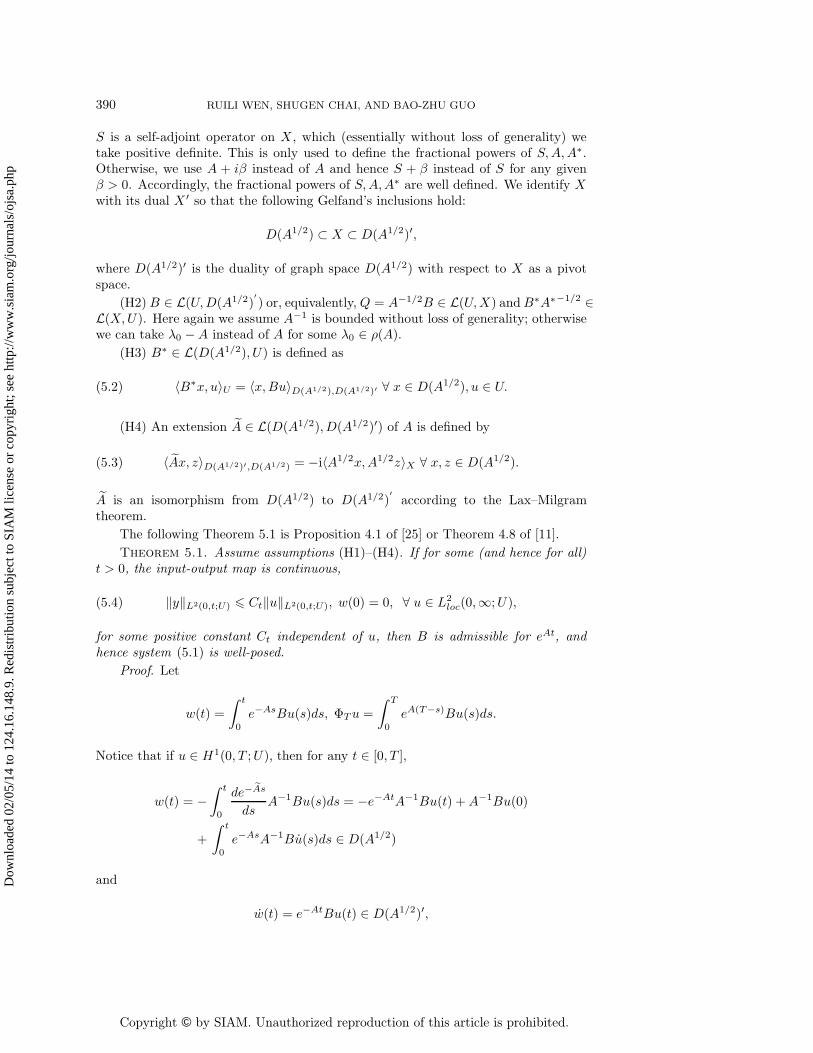
390 RUILI WEN, SHUGEN CHAI, AND BAO-ZHU GUO
S is a self-adjoint operator on X , which (essentially without loss of generality) wetake positive definite. This is only used to define the fractional powers of S,A,A∗.Otherwise, we use A + iβ instead of A and hence S + β instead of S for any givenβ > 0. Accordingly, the fractional powers of S,A,A∗ are well defined. We identify Xwith its dual X ′ so that the following Gelfand’s inclusions hold:
D(A1/2) ⊂ X ⊂ D(A1/2)′,
where D(A1/2)′ is the duality of graph space D(A1/2) with respect to X as a pivotspace.
(H2)B ∈ L(U,D(A1/2)′) or, equivalently, Q = A−1/2B ∈ L(U,X) andB∗A∗−1/2 ∈
L(X,U). Here again we assume A−1 is bounded without loss of generality; otherwisewe can take λ0 −A instead of A for some λ0 ∈ ρ(A).
(H3) B∗ ∈ L(D(A1/2), U) is defined as
(5.2) 〈B∗x, u〉U = 〈x,Bu〉D(A1/2),D(A1/2)′ ∀ x ∈ D(A1/2), u ∈ U.
(H4) An extension A ∈ L(D(A1/2), D(A1/2)′) of A is defined by
(5.3) 〈Ax, z〉D(A1/2)′,D(A1/2) = −i〈A1/2x,A1/2z〉X ∀ x, z ∈ D(A1/2).
A is an isomorphism from D(A1/2) to D(A1/2)′according to the Lax–Milgram
theorem.
The following Theorem 5.1 is Proposition 4.1 of [25] or Theorem 4.8 of [11].
Theorem 5.1. Assume assumptions (H1)–(H4). If for some (and hence for all)t > 0, the input-output map is continuous,
(5.4) ‖y‖L2(0,t;U) � Ct‖u‖L2(0,t;U), w(0) = 0, ∀ u ∈ L2loc(0,∞;U),
for some positive constant Ct independent of u, then B is admissible for eAt, andhence system (5.1) is well-posed.
Proof. Let
w(t) =
∫ t
0
e−AsBu(s)ds, ΦTu =
∫ T
0
eA(T−s)Bu(s)ds.
Notice that if u ∈ H1(0, T ;U), then for any t ∈ [0, T ],
w(t) = −∫ t
0
de− ˜As
dsA−1Bu(s)ds = −e−AtA−1Bu(t) +A−1Bu(0)
+
∫ t
0
e−AsA−1Bu(s)ds ∈ D(A1/2)
and
w(t) = e−AtBu(t) ∈ D(A1/2)′,
Dow
nloa
ded
02/0
5/14
to 1
24.1
6.14
8.9.
Red
istr
ibut
ion
subj
ect t
o SI
AM
lice
nse
or c
opyr
ight
; see
http
://w
ww
.sia
m.o
rg/jo
urna
ls/o
jsa.
php

Copyright © by SIAM. Unauthorized reproduction of this article is prohibited.
WELL-POSEDNESS AND EXACT CONTROLLABILITY 391
where eAt is the C0-semigroup generated by A on D(A1/2)′. Hence by (5.4), we have
CT ‖u‖2L2(0,T ;U) �∫ T
0
〈B∗Φtu, u(t)〉Udt
=
∫ T
0
⟨∫ t
0
eA(t−s)Bu(s)ds,Bu(t)
⟩D(A1/2),D(A1/2)′
dt
=
∫ T
0
⟨∫ t
0
e−AsBu(s)ds, e−AtBu(t)
⟩D(A1/2),D(A1/2)′
dt
=
∫ T
0
〈w(t), w(t)〉D(A1/2),D(A1/2)′ dt
=1
2
∫ T
0
d
dt〈w(t), w(t)〉Xdt = 1
2‖w(T )‖2X =
1
2
∥∥∥∥∥∫ T
0
e−AsBu(s)ds
∥∥∥∥∥2
X
=1
2
∥∥∥∥∥e−AT
∫ T
0
eA(T−s)Bu(s)ds
∥∥∥∥∥2
X
.
Therefore,∥∥∥∥∥∫ T
0
eA(T−s)Bu(s)ds
∥∥∥∥∥2
X
� ‖eAT‖∥∥∥∥∥e−AT
∫ T
0
eA(T−s)Bu(s)ds
∥∥∥∥∥2
X
� 2CT ‖eAT‖‖u‖2L2(0,T ;U).
This shows that
‖ΦTu‖X � CT ‖u‖L2(0,T ;U) ∀ u ∈ H1(0, T ;U).
Since H1(0, T ;U) is dense in L2(0, T ;U), we thus obtain
ΦT ∈ L(L2(0, T ;U), X).
In other words, B is admissible to eAt and so is for B∗ to eA∗t. This proves the
required result.
The following Theorem 5.2 is Theorem 5.8 of [11].
Theorem 5.2. Under the assumption of Theorem 5.1, the system (5.1) is regularand the feedthrough operator is zero.
Proof. By Theorem 5.8 of [35], it suffices to show that for any u ∈ U ,
A−1Bu ∈ D(B∗Λ),
where B∗Λ is the Λ-extension of B∗|D(A), which is defined as
(5.5) B∗Λx = lim
λ→+∞B∗|D(A)λ(λ −A)−1x ∀ x ∈ D(B∗
Λ)
whenever the limit exists. Now since A is the generator of a C0-semigroup,
limλ→+∞
λ(λ −A)−1x = x ∀ x ∈ X.
Dow
nloa
ded
02/0
5/14
to 1
24.1
6.14
8.9.
Red
istr
ibut
ion
subj
ect t
o SI
AM
lice
nse
or c
opyr
ight
; see
http
://w
ww
.sia
m.o
rg/jo
urna
ls/o
jsa.
php

Copyright © by SIAM. Unauthorized reproduction of this article is prohibited.
392 RUILI WEN, SHUGEN CHAI, AND BAO-ZHU GUO
Hence for any x ∈ D(A1/2), since B∗Λ = B∗ in D(A) and B∗A−1/2 is bounded, we
have
limλ→+∞
B∗|D(A)λ(λ −A)−1x = limλ→+∞
B∗λ(λ −A)−1x
= limλ→+∞
B∗A−1/2λ(λ −A)−1A1/2x = B∗x.
Therefore,
(5.6) D(A1/2) ⊂ D(B∗Λ) and B
∗Λ = B∗ in D(A1/2).
So system (5.1) is regular. By the appendix of [12], the transfer function of system(5.1) is
(5.7) G(s) = B∗(s−A)−1B,
which shows that the feedthrough operator D = 0 by the formula of [35] that
G(s) = B∗Λ(s−A)−1B +D.
The following proposition is Proposition 2.1 of [24] and Proposition 6.4 of [11].Proposition 5.3. Assume assumptions (H1)–(H4). Define the proportional out-
put feedback control operator as follows:
(5.8) AFx = (A−BB∗)x ∀ x ∈ D(AF ) = {x ∈ D(A1/2)|(A−BB∗)x ∈ X}.
Then(i) D(AF ) = D(A1/2(I − iQQ∗)A1/2) ⊂ D(A1/2) ⊂ D(B∗), A−1
F = A−1/2
(I − iQQ∗)−1A−1/2, where Q = A−1/2B ∈ L(U,X).(ii) A∗
Fx = (−A−BB∗)x ∀ x ∈ D(A∗F ) = {x ∈ D(A1/2)|(−A−BB∗)x ∈ X}.
(iii) AF generates a C0-semigroup of contractions on X.Proof. For any x ∈ D(AF ),
AFx = (A−BB∗)x = A1/2[I − (A−1/2B)(B∗A−1/2)]A1/2x = A1/2(I − iQQ∗)A1/2x,
where Q = A−1/2B ∈ L(U,X) and Q∗ = B∗A∗−1/2 ∈ L(X,U) is the adjoint oper-
ator of Q due to A∗ = −A. Hence A∗1/2 = iA1/2, A∗−1/2 = −iA−1/2, B∗A−1/2 =iB∗A∗−1/2 = iQ∗. Since QQ∗ ∈ L(X) is obviously nonnegative, I − iQQ∗ is boundedinvertible. Hence A−1
F = A−1/2(I − iQQ∗)−1A−1/2. This is (i). By A∗F−1 =
−A−1/2(I + iQQ∗)−1A−1/2, we have A∗F = −A1/2(I + iQQ∗)A1/2 = −A − BB∗,
which is just (ii).Now we show that AF is dissipative. Actually, for any x ∈ D(AF ), by (5.2)
and (5.3),
Re〈AFx, x〉 = Re〈(A −BB∗)x, x〉(5.9)
= Re(−i)‖A1/2x‖2 − ‖B∗x‖2 = −‖B∗x‖2 � 0.
Since A−1F is bounded, it follows from the Lummer–Phillips theorem [28, Theorem
1.3.6] that AF generates a C0-semigroup of contractions on X .The following theorem, which is Theorem 6.7 of [11], is called Russell’s principle
for the first order system (5.1) [31].
Dow
nloa
ded
02/0
5/14
to 1
24.1
6.14
8.9.
Red
istr
ibut
ion
subj
ect t
o SI
AM
lice
nse
or c
opyr
ight
; see
http
://w
ww
.sia
m.o
rg/jo
urna
ls/o
jsa.
php

Copyright © by SIAM. Unauthorized reproduction of this article is prohibited.
WELL-POSEDNESS AND EXACT CONTROLLABILITY 393
Theorem 5.4. Assume assumptions (H1)–(H4). If the operator AF in Proposi-tion 5.3 generates an exponential stable C0-semigroup on X, then the system (5.1) isexactly controllable.
Proof. First, by Proposition 5.3, the closed-loop system
(5.10) w(t) = AFw(t) = Aw(t) −BB∗w(t), w(0) = w0
associates with a C0-semigroup solution. For any w0 ∈ D(AF ), w ∈ D(AF ) ⊂D(A1/2) ⊂ D(B∗), take the inner product with w on both sides of (5.10) and take(5.9) into account to get the energy identity:
(5.11) 2
∫ t
0
‖B∗w(s)‖2ds = ‖w0‖2 − ‖w(t)‖2 � ‖w0‖2 ∀ w0 ∈ D(AF ), t > 0.
Since D(AF ) is dense in X , we suppose (5.11) to make sense for any w0 ∈ X , that is,for any w0 ∈ X, t > 0, B∗w ∈ L2(0, t;U). Since eAF t is exponentially stable and so iseA
∗F t, there exists a T0 > 0 such that for all T > T0,
(5.12) ‖eA∗FT ‖ < 1.
Owing to (5.11), for any initial value w0 ∈ X , we can also suppose the solution of(5.10) to be
w(t) = eAtw0 +
∫ t
0
eA(t−s)Bu1(s)ds = eAtw0 +Φtu1 ∈ C(0, T ;X),(5.13)
u1 = −B∗w ∈ L2(0, T ;U).
Next, consider the equation
(5.14) z = −A∗F z, z(T ) = w(T ),
where w is the solution to (5.10). Let η(t) = z(T − t). Then η satisfies
(5.15) η = A∗F η, η(0) = w(T ).
By energy identity (5.11), the solution to (5.15) satisfies η ∈ C(0, T ;X) and B∗η ∈L2(0, T ;U). Hence z ∈ C(0, T ;X), u2 = B∗z ∈ L2(0, T ;U). Same to (5.13), thesolution of (5.14) can be understood as
(5.16)
z(t) = eAtz(0) +
∫ t
0
eA(t−s)Bu2(s)ds = eAtz(0) + Φtu2, u2 = B∗z ∈ L2(0, T ;U).
Let x = w − z ∈ C(0, T ;X), u = u1 − u2 ∈ L2(0, T ;U). By (5.13) and (5.16), itfollows that
(5.17) x(t) = eAt[w0 − z(0)] + Φtu, x(T ) = 0.
Since A generates a C0-group, the exact controllability of system (5.1) is equivalentto the null controllability. So we need only prove that for any x0 ∈ X , there exists aw0 ∈ X such that
(5.18) w0 − z(0) = x0.
Dow
nloa
ded
02/0
5/14
to 1
24.1
6.14
8.9.
Red
istr
ibut
ion
subj
ect t
o SI
AM
lice
nse
or c
opyr
ight
; see
http
://w
ww
.sia
m.o
rg/jo
urna
ls/o
jsa.
php

Copyright © by SIAM. Unauthorized reproduction of this article is prohibited.
394 RUILI WEN, SHUGEN CHAI, AND BAO-ZHU GUO
To this end, by (5.15)
η(t) = eA∗F tw(T )
and by (5.12),
‖z(0)‖ � ‖eA∗FT ‖‖w(T )‖ � ‖eA∗
FT ‖2‖w0‖.So the mapping
w0 → z(0) = Pw0
is a contraction mapping. Therefore,
w0 − z(0) = (I − P)w0 = x0
admits a unique solution:
w0 = (I − P)−1x0.
Remark 5.1. From the proof of Theorem 5.4, we do not even need the admissibilityof B. The energy identity (5.11) shows that for the system
(5.19)
{w(t) = AFw(t),yw(t) = B∗w,
the output operator is always admissible.The following result, which is Theorem 6.8 of [11] or the proposition 6.1.13 of
[34] shows that the reverse of Theorem 5.4 is also true provided that system (5.1) iswell-posed.
Theorem 5.5. Assume assumptions (H1)–(H4). If the open-loop system of (5.1)is well-posed and exactly controllable, then the operator AF defined by (5.8) generatesan exponential stable C0-semigroup on X.
Proof. By Theorem 5.2 and the well-posedness assumption, system (5.1) is regularand the feedthrough operator is zero. We write the solution of the closed-loop system(5.10) as
(5.20) eAF tw0 = eAtw0 − ΦtB∗eAF ·w0 ∈ D(AF ) ⊂ D(A1/2) ∀ w0 ∈ D(AF ).
By (5.6) and
(Ftu)(t) = B∗Λ
∫ t
0
T (t− s)Bu(s)ds ∀ t � 0 a.e., u ∈ L2loc(0,∞;U),(5.21)
B∗Λe
Atw0 = B∗eAF tw0 + FtB∗eAF ·w0 ∀ w0 ∈ D(AF ),(5.22)
where Ft is the input-output map of system (5.1) [5]. Since the system (5.1) is supposedto be well-posed, for any T > 0, FT ∈ L(L2(0, T ;U)). Set cT = ‖FT ‖. By (5.11),
(5.23) ‖B∗Λe
A·w0‖L2(0,T ;U) � (1 + cT )‖B∗eAF ·w0‖L2(0,T ;U) ∀ w0 ∈ D(AF ).
Since A∗ = −A and the assumption of well-posedness, the exact controllability ofsystem (5.1) is equivalent to its exact observability [34, Theorem 11.2.1]. So thereexists a DT > 0 such that
‖w0‖2 � DT
∫ T
0
‖B∗Λe
Atw0‖2Udt(5.24)
� DT (1 + cT )2
∫ T
0
‖B∗eAF tw0‖2Udt ∀ w0 ∈ D(AF ).
Dow
nloa
ded
02/0
5/14
to 1
24.1
6.14
8.9.
Red
istr
ibut
ion
subj
ect t
o SI
AM
lice
nse
or c
opyr
ight
; see
http
://w
ww
.sia
m.o
rg/jo
urna
ls/o
jsa.
php

Copyright © by SIAM. Unauthorized reproduction of this article is prohibited.
WELL-POSEDNESS AND EXACT CONTROLLABILITY 395
On the other hand, by the energy identity (5.11) and (5.24), for any w0 ∈ D(AF ),
‖eAFTw0‖2 � ‖w0‖2 � DT (1 + cT )2
∫ T
0
‖B∗eAF tw0‖2Udt
=1
2DT (1 + cT )
2[‖w0‖2 − ‖eAFTw0‖2].
Hence
(5.25) ‖eAFTw0‖2 � DT (1 + cT )2
2 +DT (1 + cT )2‖w0‖2 ∀ w0 ∈ D(AF ).
Since D(AF ) is dense in X , (5.25) shows that ‖eAFT ‖ < 1. Therefore eAF t is expo-nentially stable on X .
Acknowledgment. The authors would like to thank anonymous referees andeditors for their careful reading and helpful suggestions for the improvement of themanuscript.
REFERENCES
[1] K. Ammari, Dirichlet boundary stabilization of the wave equation, Asymptot. Anal., 30 (2002),pp. 117–130.
[2] K. Ammari and M. Tucsnak, Stabilization of second-order evolution equations by a class ofunbounded feedbacks, ESAIM Control Optim. Calc. Var., 6 (2001), pp. 361–386.
[3] C. Bardos, G. Lebeau, and R. Rauch, Controle et stabilisation de l’equation des ondes,Publication de l’Ecole Polytechnique Palaiseau, Palaiseau, France, 1987.
[4] C. I. Byrnes, D. S. Gilliam, V. I. Shubov, and G. Weiss, Regular linear systems governedby a boundary controlled heat equation, J. Dyn. Control Syst., 8 (2002), pp. 341–370.
[5] R. F. Curtain, The Salamon-Weiss class of well-posed infinite dimensional linear systems:A survey, IMA J. Math. Control Inform., 14 (1997), pp. 207–223.
[6] R. F. Curtain, Linear operator inequalities for strongly stable weakly regular linear systems,Math. Control Signals Systems, 14 (2001), pp. 299–337.
[7] R. F. Curtain and G. Weiss, Well-posedness of triples of operators (in the sense of linearsystems theory), in Control and Estimation of Distributed Parameter Systems, F. Kappel,K. Kunisch, and W. Schappacher eds., Birkhauser, Basel, 1989, pp. 41–59.
[8] R. F. Curtain and G. Weiss, Exponential stabilization of well-posed systems by collocatedfeedback, SIAM J. Control Optim., 45 (2006), pp. 273–297.
[9] S. G. Chai and B. Z. Guo, Well-posedness and regularity of weakly coupled wave-plate equationwith boundary control and observation, J. Dyn. Control Syst., 15 (2009), pp. 331–358.
[10] S. G. Chai and B. Z. Guo, Feedthrough operator for linear elasticity system with boundarycontrol and observation, SIAM J. Control Optim., 48 (2010), pp. 3708–3734.
[11] B. Z. Guo and S. G. Chai, Infinite-Dimensional Linear System Control Theory, Science Press,Beijing, 2012 (in Chinese).
[12] B. Z. Guo and Y. H. Luo, Controllability and stability of a second order hyperbolic systemwith collocated sensor/actuator, Systems Control Lett., 46 (2002), pp. 45–65.
[13] B. Z. Guo and Z. C. Shao, Regularity of a Schrodinger equation with Dirichlet control andcollocated observation, Systems Control Lett., 54 (2005), pp. 1135–1142.
[14] B. Z. Guo and Z. C. Shao, Regularity of an Euler-Bernoulli equation with Neumann controland collocated observation, J. Dyn. Control Syst., 12 (2006), pp. 405–418.
[15] B. Z. Guo and X. Zhang, The regularity of the wave equation with partial Dirichlet controland collocated observation, SIAM J. Control Optim., 44 (2005), pp. 1598–1613.
[16] C. Hao, L. Hsiao, and B. Wang, Wellposedness for the fourth order nonlinear Schrodingerequations, J. Math. Anal. Appl., 320 (2006), pp. 246–265.
[17] C. Hao, L. Hsiao, and B. Wang, Well-posedness of Cauchy problem for the fourth ordernonlinear Schrodinger equations in multi-dimensional spaces, J. Math. Anal. Appl., 328(2007), pp. 58–83.
[18] L. Hormander, Linear Partial Differential Operators, Springer-Verlag, Berlin, 1969.[19] V. I. Karpman, Stabilization of soliton instabilities by higher-order dispersion: Fourth-order
nonlinear Schrodinger-type equations, Phys. Rev. E, 53 (1996), pp. 1336–1339.
Dow
nloa
ded
02/0
5/14
to 1
24.1
6.14
8.9.
Red
istr
ibut
ion
subj
ect t
o SI
AM
lice
nse
or c
opyr
ight
; see
http
://w
ww
.sia
m.o
rg/jo
urna
ls/o
jsa.
php

Copyright © by SIAM. Unauthorized reproduction of this article is prohibited.
396 RUILI WEN, SHUGEN CHAI, AND BAO-ZHU GUO
[20] V. I. Karpman and A. G. Shagalov, Stability of solitons described by nonlinear Schrodinger-type equations with higher-order dispersion, Phys. Rev. D, 144 (2000), pp. 194–210.
[21] V. Komornik, Exact Controllability and Stabilization: The Multiplier Method, John Wiley,Chichester, 1994.
[22] I. Lasiecka, Exponential decay rates for the solutions of Euler-Bernoulli equations withboundary dissipation occurring in the Moments only, J. Differential Equations, 95 (1992),pp. 169–182.
[23] I. Lasiecka and R. Triggiani, Optimal regularity, exact controllability and uniform stabi-lization of Schrodinger equations with Dirichlet control, Differential Integral Equations,5 (1992), pp. 521–535.
[24] I. Lasiecka and R. Triggiani, L2(Σ)-regularity of the boundary to boundary operator B∗Lfor hyperbolic and Petrowski PDEs, Abstr. Appl. Anal., 19 (2003), pp. 1061–1139.
[25] I. Lasiecka and R. Triggiani, The operator B∗L for the wave equation with Dirichlet control,Abstr. Appl. Anal., 7 (2004), pp. 625–634.
[26] J. L. Lions and E. Magens, Non-Homegeneous Boundary-Valued Problems and Applications,Springer-Verlag, Berlin, 1972.
[27] J. L. Lions, Exact contrllability, stabilization and perturbations for distributed systems, SIAMRev., 30 (1988), pp. 1–68.
[28] A. Pazy, Semigroups of Linear Operators and Applications to Partial Differential Equations,Springer-Verlag, New York, 1983.
[29] B. Pausader, Global well-posedness for energy critical fourth-order Schrodinger equations inthe radial case, Dyn. Partial Differ. Equ., 4 (2007), pp. 197–225.
[30] B. Pausader, The cubic fourth-order Schrodinger equation, J. Funct. Anal., 256 (2009),pp. 2473–2517.
[31] D. L. Russell, Exact boundary value controllability theorems for wave and heat processesin star complemented regions, in Differential Games and Control Theory, E. O. Roxin,P. T. Liu, and R. L. Sternberg, eds., Lecture Notes in Pure and Appl. Math. 10, MarcelDekker, New York, 1974, pp. 291–319.
[32] O. J. Staffans, Well-Posed Linear Systems, Cambridge University Press, Cambridge, UK,2005.
[33] O. J. Staffans and G. Weiss, A physically motivated class of scattering passive linear systems,SIAM J. Control Optim., 50 (2012), pp. 3083–3112.
[34] M. Tucsnak and G. Weiss, Observation and Control for Operator Semigroups, Birkhauser,Basel, 2009.
[35] G. Weiss, Transfer functions of regular linear systems, Part I: Characterizations of regularity,Trans. Amer. Math. Soc., 342 (1994), pp. 827–854.
[36] G. Weiss and R. F. Curtain, Dynamic stabilization of regular linear systems, IEEE Trans.Automat. Control, 42 (1997), pp. 4–21.
[37] G. Weiss, O. J. Staffans, and M. Tucsnak, Well-posed linear systems: A survey with em-phasis on conservative systems, Int. J. Appl. Math. Comput. Sci., 11 (2001), pp. 7–33.
[38] C. Zheng and Z. C. Zhou, Exact controllability for the fourth order Schrodinger equation,Chinese Ann. Math. Ser. B, 33 (2012), pp. 395–404.
[39] H. Zwart, Transfer functions for infinite-dimensional systems, Systems Control Lett., 52(2004), pp. 247–255.
Dow
nloa
ded
02/0
5/14
to 1
24.1
6.14
8.9.
Red
istr
ibut
ion
subj
ect t
o SI
AM
lice
nse
or c
opyr
ight
; see
http
://w
ww
.sia
m.o
rg/jo
urna
ls/o
jsa.
php
![Well-Posedness of Nonlinear Schr¨odinger EquationsUnconditionally well-posed Kato [28] introduces the concept of unconditional well-posedness of nonlinear Schr¨odinger equation.](https://static.fdocuments.in/doc/165x107/5e7d7c75391fca0b2915e5dd/well-posedness-of-nonlinear-schrodinger-equations-unconditionally-well-posed-kato.jpg)


![The Active Disturbance Rejection Control to Stabilization ...lsc.amss.ac.cn/~bzguo/papers/Zhouhc.pdf · one-dimensional partial differential equations (PDEs) are also availableinourrecentworks[10]–[12]buttheADRCformulti-dimensional](https://static.fdocuments.in/doc/165x107/6103804be42ab4682305be80/the-active-disturbance-rejection-control-to-stabilization-lscamssaccnbzguopapers.jpg)

