WellfoundednessFrom Wikipedia, the free encyclopedia

Contents

1 Ascending chain condition 11.1 Definition . . . . . . . . . . . . . . . . . . . . . . . . . . . . . . . . . . . . . . . . . . . . . . . 1

1.1.1 Comments . . . . . . . . . . . . . . . . . . . . . . . . . . . . . . . . . . . . . . . . . . 11.2 See also . . . . . . . . . . . . . . . . . . . . . . . . . . . . . . . . . . . . . . . . . . . . . . . . 21.3 Notes . . . . . . . . . . . . . . . . . . . . . . . . . . . . . . . . . . . . . . . . . . . . . . . . . 21.4 References . . . . . . . . . . . . . . . . . . . . . . . . . . . . . . . . . . . . . . . . . . . . . . 2

2 Axiom of limitation of size 32.1 History . . . . . . . . . . . . . . . . . . . . . . . . . . . . . . . . . . . . . . . . . . . . . . . . . 32.2 Zermelo’s models and the axiom of limitation of size . . . . . . . . . . . . . . . . . . . . . . . . . 4

2.2.1 The model Vω . . . . . . . . . . . . . . . . . . . . . . . . . . . . . . . . . . . . . . . . 42.2.2 The models Vκ where κ is a strongly inaccessible cardinal . . . . . . . . . . . . . . . . . . 5

2.3 See also . . . . . . . . . . . . . . . . . . . . . . . . . . . . . . . . . . . . . . . . . . . . . . . . 62.4 Notes . . . . . . . . . . . . . . . . . . . . . . . . . . . . . . . . . . . . . . . . . . . . . . . . . 62.5 References . . . . . . . . . . . . . . . . . . . . . . . . . . . . . . . . . . . . . . . . . . . . . . 7

3 Axiom of regularity 93.1 Elementary implications of regularity . . . . . . . . . . . . . . . . . . . . . . . . . . . . . . . . . 9

3.1.1 No set is an element of itself . . . . . . . . . . . . . . . . . . . . . . . . . . . . . . . . . 93.1.2 No infinite descending sequence of sets exists . . . . . . . . . . . . . . . . . . . . . . . . 93.1.3 Simpler set-theoretic definition of the ordered pair . . . . . . . . . . . . . . . . . . . . . . 103.1.4 Every set has an ordinal rank . . . . . . . . . . . . . . . . . . . . . . . . . . . . . . . . . 103.1.5 For every two sets, only one can be an element of the other . . . . . . . . . . . . . . . . . 10

3.2 The axiom of dependent choice and no infinite descending sequence of sets implies regularity . . . . 103.3 Regularity and the rest of ZF(C) axioms . . . . . . . . . . . . . . . . . . . . . . . . . . . . . . . 103.4 Regularity and Russell’s paradox . . . . . . . . . . . . . . . . . . . . . . . . . . . . . . . . . . . 103.5 Regularity, the cumulative hierarchy, and types . . . . . . . . . . . . . . . . . . . . . . . . . . . 113.6 History . . . . . . . . . . . . . . . . . . . . . . . . . . . . . . . . . . . . . . . . . . . . . . . . 113.7 See also . . . . . . . . . . . . . . . . . . . . . . . . . . . . . . . . . . . . . . . . . . . . . . . . 123.8 References . . . . . . . . . . . . . . . . . . . . . . . . . . . . . . . . . . . . . . . . . . . . . . 123.9 External links . . . . . . . . . . . . . . . . . . . . . . . . . . . . . . . . . . . . . . . . . . . . . 13

4 Better-quasi-ordering 14

i

ii CONTENTS

4.1 Motivation . . . . . . . . . . . . . . . . . . . . . . . . . . . . . . . . . . . . . . . . . . . . . . 144.2 Definition . . . . . . . . . . . . . . . . . . . . . . . . . . . . . . . . . . . . . . . . . . . . . . . 144.3 Simpson’s alternative definition . . . . . . . . . . . . . . . . . . . . . . . . . . . . . . . . . . . . 144.4 Major theorems . . . . . . . . . . . . . . . . . . . . . . . . . . . . . . . . . . . . . . . . . . . . 154.5 See also . . . . . . . . . . . . . . . . . . . . . . . . . . . . . . . . . . . . . . . . . . . . . . . . 154.6 References . . . . . . . . . . . . . . . . . . . . . . . . . . . . . . . . . . . . . . . . . . . . . . . 15

5 Dickson’s lemma 165.1 Example . . . . . . . . . . . . . . . . . . . . . . . . . . . . . . . . . . . . . . . . . . . . . . . . 165.2 Formal statement . . . . . . . . . . . . . . . . . . . . . . . . . . . . . . . . . . . . . . . . . . . 165.3 Generalizations and applications . . . . . . . . . . . . . . . . . . . . . . . . . . . . . . . . . . . . 165.4 See also . . . . . . . . . . . . . . . . . . . . . . . . . . . . . . . . . . . . . . . . . . . . . . . . 175.5 References . . . . . . . . . . . . . . . . . . . . . . . . . . . . . . . . . . . . . . . . . . . . . . . 18

6 Epsilon-induction 196.1 See also . . . . . . . . . . . . . . . . . . . . . . . . . . . . . . . . . . . . . . . . . . . . . . . . 19

7 Friedman’s SSCG function 207.1 See also . . . . . . . . . . . . . . . . . . . . . . . . . . . . . . . . . . . . . . . . . . . . . . . . 207.2 References . . . . . . . . . . . . . . . . . . . . . . . . . . . . . . . . . . . . . . . . . . . . . . 20

8 Higman’s lemma 218.1 References . . . . . . . . . . . . . . . . . . . . . . . . . . . . . . . . . . . . . . . . . . . . . . . 21

9 Infinite descending chain 229.1 See also . . . . . . . . . . . . . . . . . . . . . . . . . . . . . . . . . . . . . . . . . . . . . . . . 229.2 References . . . . . . . . . . . . . . . . . . . . . . . . . . . . . . . . . . . . . . . . . . . . . . . 22

10 Kleene–Brouwer order 2310.1 Definition . . . . . . . . . . . . . . . . . . . . . . . . . . . . . . . . . . . . . . . . . . . . . . . 2310.2 Tree interpretation . . . . . . . . . . . . . . . . . . . . . . . . . . . . . . . . . . . . . . . . . . . 2310.3 Recursion theory . . . . . . . . . . . . . . . . . . . . . . . . . . . . . . . . . . . . . . . . . . . 2410.4 History . . . . . . . . . . . . . . . . . . . . . . . . . . . . . . . . . . . . . . . . . . . . . . . . . 2410.5 References . . . . . . . . . . . . . . . . . . . . . . . . . . . . . . . . . . . . . . . . . . . . . . 24

11 Kruskal’s tree theorem 2511.1 Friedman’s finite form . . . . . . . . . . . . . . . . . . . . . . . . . . . . . . . . . . . . . . . . . 2511.2 See also . . . . . . . . . . . . . . . . . . . . . . . . . . . . . . . . . . . . . . . . . . . . . . . . 2611.3 Notes . . . . . . . . . . . . . . . . . . . . . . . . . . . . . . . . . . . . . . . . . . . . . . . . . 2611.4 References . . . . . . . . . . . . . . . . . . . . . . . . . . . . . . . . . . . . . . . . . . . . . . 26

12 König’s lemma 2712.1 Statement of the lemma . . . . . . . . . . . . . . . . . . . . . . . . . . . . . . . . . . . . . . . . 27

12.1.1 Proof . . . . . . . . . . . . . . . . . . . . . . . . . . . . . . . . . . . . . . . . . . . . . 27

CONTENTS iii

12.2 Computability aspects . . . . . . . . . . . . . . . . . . . . . . . . . . . . . . . . . . . . . . . . . 2812.3 Relationship to constructive mathematics and compactness . . . . . . . . . . . . . . . . . . . . . . 2912.4 Relationship with the axiom of choice . . . . . . . . . . . . . . . . . . . . . . . . . . . . . . . . . 2912.5 See also . . . . . . . . . . . . . . . . . . . . . . . . . . . . . . . . . . . . . . . . . . . . . . . . 3012.6 Notes . . . . . . . . . . . . . . . . . . . . . . . . . . . . . . . . . . . . . . . . . . . . . . . . . 3012.7 References . . . . . . . . . . . . . . . . . . . . . . . . . . . . . . . . . . . . . . . . . . . . . . . 3012.8 External links . . . . . . . . . . . . . . . . . . . . . . . . . . . . . . . . . . . . . . . . . . . . . 31

13 Mostowski collapse lemma 3213.1 Statement . . . . . . . . . . . . . . . . . . . . . . . . . . . . . . . . . . . . . . . . . . . . . . . 3213.2 Generalizations . . . . . . . . . . . . . . . . . . . . . . . . . . . . . . . . . . . . . . . . . . . . 3213.3 Application . . . . . . . . . . . . . . . . . . . . . . . . . . . . . . . . . . . . . . . . . . . . . . 3213.4 References . . . . . . . . . . . . . . . . . . . . . . . . . . . . . . . . . . . . . . . . . . . . . . 33

14 Newman’s lemma 3414.1 Diamond lemma . . . . . . . . . . . . . . . . . . . . . . . . . . . . . . . . . . . . . . . . . . . . 3414.2 Notes . . . . . . . . . . . . . . . . . . . . . . . . . . . . . . . . . . . . . . . . . . . . . . . . . 3414.3 References . . . . . . . . . . . . . . . . . . . . . . . . . . . . . . . . . . . . . . . . . . . . . . . 35

14.3.1 Textbooks . . . . . . . . . . . . . . . . . . . . . . . . . . . . . . . . . . . . . . . . . . 3514.4 External links . . . . . . . . . . . . . . . . . . . . . . . . . . . . . . . . . . . . . . . . . . . . . 35

15 Noetherian topological space 3615.1 Definition . . . . . . . . . . . . . . . . . . . . . . . . . . . . . . . . . . . . . . . . . . . . . . . 3615.2 Relation to compactness . . . . . . . . . . . . . . . . . . . . . . . . . . . . . . . . . . . . . . . 3615.3 Noetherian topological spaces from algebraic geometry . . . . . . . . . . . . . . . . . . . . . . . 3615.4 Example . . . . . . . . . . . . . . . . . . . . . . . . . . . . . . . . . . . . . . . . . . . . . . . 3715.5 References . . . . . . . . . . . . . . . . . . . . . . . . . . . . . . . . . . . . . . . . . . . . . . . 37

16 Non-well-founded set theory 3816.1 Details . . . . . . . . . . . . . . . . . . . . . . . . . . . . . . . . . . . . . . . . . . . . . . . . 3816.2 Applications . . . . . . . . . . . . . . . . . . . . . . . . . . . . . . . . . . . . . . . . . . . . . . 3916.3 See also . . . . . . . . . . . . . . . . . . . . . . . . . . . . . . . . . . . . . . . . . . . . . . . . 3916.4 Notes . . . . . . . . . . . . . . . . . . . . . . . . . . . . . . . . . . . . . . . . . . . . . . . . . 3916.5 References . . . . . . . . . . . . . . . . . . . . . . . . . . . . . . . . . . . . . . . . . . . . . . 4016.6 Further reading . . . . . . . . . . . . . . . . . . . . . . . . . . . . . . . . . . . . . . . . . . . . 4016.7 External links . . . . . . . . . . . . . . . . . . . . . . . . . . . . . . . . . . . . . . . . . . . . . 40

17 Ordinal number 4117.1 Ordinals extend the natural numbers . . . . . . . . . . . . . . . . . . . . . . . . . . . . . . . . . 4217.2 Definitions . . . . . . . . . . . . . . . . . . . . . . . . . . . . . . . . . . . . . . . . . . . . . . 44

17.2.1 Well-ordered sets . . . . . . . . . . . . . . . . . . . . . . . . . . . . . . . . . . . . . . . 4417.2.2 Definition of an ordinal as an equivalence class . . . . . . . . . . . . . . . . . . . . . . . 4417.2.3 Von Neumann definition of ordinals . . . . . . . . . . . . . . . . . . . . . . . . . . . . . 44

iv CONTENTS

17.2.4 Other definitions . . . . . . . . . . . . . . . . . . . . . . . . . . . . . . . . . . . . . . . 4517.3 Transfinite sequence . . . . . . . . . . . . . . . . . . . . . . . . . . . . . . . . . . . . . . . . . . 4517.4 Transfinite induction . . . . . . . . . . . . . . . . . . . . . . . . . . . . . . . . . . . . . . . . . 45

17.4.1 What is transfinite induction? . . . . . . . . . . . . . . . . . . . . . . . . . . . . . . . . 4517.4.2 Transfinite recursion . . . . . . . . . . . . . . . . . . . . . . . . . . . . . . . . . . . . . 4617.4.3 Successor and limit ordinals . . . . . . . . . . . . . . . . . . . . . . . . . . . . . . . . . 4617.4.4 Indexing classes of ordinals . . . . . . . . . . . . . . . . . . . . . . . . . . . . . . . . . 4617.4.5 Closed unbounded sets and classes . . . . . . . . . . . . . . . . . . . . . . . . . . . . . . 47

17.5 Arithmetic of ordinals . . . . . . . . . . . . . . . . . . . . . . . . . . . . . . . . . . . . . . . . 4717.6 Ordinals and cardinals . . . . . . . . . . . . . . . . . . . . . . . . . . . . . . . . . . . . . . . . 47

17.6.1 Initial ordinal of a cardinal . . . . . . . . . . . . . . . . . . . . . . . . . . . . . . . . . . 4817.6.2 Cofinality . . . . . . . . . . . . . . . . . . . . . . . . . . . . . . . . . . . . . . . . . . . 48

17.7 Some “large” countable ordinals . . . . . . . . . . . . . . . . . . . . . . . . . . . . . . . . . . . 4817.8 Topology and ordinals . . . . . . . . . . . . . . . . . . . . . . . . . . . . . . . . . . . . . . . . 4917.9 Downward closed sets of ordinals . . . . . . . . . . . . . . . . . . . . . . . . . . . . . . . . . . . 4917.10See also . . . . . . . . . . . . . . . . . . . . . . . . . . . . . . . . . . . . . . . . . . . . . . . . 4917.11Notes . . . . . . . . . . . . . . . . . . . . . . . . . . . . . . . . . . . . . . . . . . . . . . . . . 4917.12References . . . . . . . . . . . . . . . . . . . . . . . . . . . . . . . . . . . . . . . . . . . . . . . 4917.13External links . . . . . . . . . . . . . . . . . . . . . . . . . . . . . . . . . . . . . . . . . . . . . 50

18 Prewellordering 5118.1 Prewellordering property . . . . . . . . . . . . . . . . . . . . . . . . . . . . . . . . . . . . . . . 51

18.1.1 Examples . . . . . . . . . . . . . . . . . . . . . . . . . . . . . . . . . . . . . . . . . . . 5118.1.2 Consequences . . . . . . . . . . . . . . . . . . . . . . . . . . . . . . . . . . . . . . . . . 51

18.2 See also . . . . . . . . . . . . . . . . . . . . . . . . . . . . . . . . . . . . . . . . . . . . . . . . 5218.3 References . . . . . . . . . . . . . . . . . . . . . . . . . . . . . . . . . . . . . . . . . . . . . . 52

19 Robertson–Seymour theorem 5319.1 Statement . . . . . . . . . . . . . . . . . . . . . . . . . . . . . . . . . . . . . . . . . . . . . . . 5319.2 Forbidden minor characterizations . . . . . . . . . . . . . . . . . . . . . . . . . . . . . . . . . . 5419.3 Examples of minor-closed families . . . . . . . . . . . . . . . . . . . . . . . . . . . . . . . . . . 5419.4 Obstruction sets . . . . . . . . . . . . . . . . . . . . . . . . . . . . . . . . . . . . . . . . . . . . 5419.5 Polynomial time recognition . . . . . . . . . . . . . . . . . . . . . . . . . . . . . . . . . . . . . . 5519.6 Fixed-parameter tractability . . . . . . . . . . . . . . . . . . . . . . . . . . . . . . . . . . . . . . 5619.7 Finite form of the graph minor theorem . . . . . . . . . . . . . . . . . . . . . . . . . . . . . . . . 5619.8 See also . . . . . . . . . . . . . . . . . . . . . . . . . . . . . . . . . . . . . . . . . . . . . . . . 5619.9 Notes . . . . . . . . . . . . . . . . . . . . . . . . . . . . . . . . . . . . . . . . . . . . . . . . . 5619.10References . . . . . . . . . . . . . . . . . . . . . . . . . . . . . . . . . . . . . . . . . . . . . . . 5719.11External links . . . . . . . . . . . . . . . . . . . . . . . . . . . . . . . . . . . . . . . . . . . . . 57

20 Scott–Potter set theory 5820.1 ZU etc. . . . . . . . . . . . . . . . . . . . . . . . . . . . . . . . . . . . . . . . . . . . . . . . . 58

CONTENTS v

20.1.1 Preliminaries . . . . . . . . . . . . . . . . . . . . . . . . . . . . . . . . . . . . . . . . . 5820.1.2 Axioms . . . . . . . . . . . . . . . . . . . . . . . . . . . . . . . . . . . . . . . . . . . . 5920.1.3 Further existence premises . . . . . . . . . . . . . . . . . . . . . . . . . . . . . . . . . . 59

20.2 Discussion . . . . . . . . . . . . . . . . . . . . . . . . . . . . . . . . . . . . . . . . . . . . . . . 6020.2.1 Scott’s theory . . . . . . . . . . . . . . . . . . . . . . . . . . . . . . . . . . . . . . . . . 6020.2.2 Potter’s theory . . . . . . . . . . . . . . . . . . . . . . . . . . . . . . . . . . . . . . . . . 60

20.3 See also . . . . . . . . . . . . . . . . . . . . . . . . . . . . . . . . . . . . . . . . . . . . . . . . 6120.4 References . . . . . . . . . . . . . . . . . . . . . . . . . . . . . . . . . . . . . . . . . . . . . . . 6120.5 External links . . . . . . . . . . . . . . . . . . . . . . . . . . . . . . . . . . . . . . . . . . . . . 62

21 Structural induction 6321.1 Examples . . . . . . . . . . . . . . . . . . . . . . . . . . . . . . . . . . . . . . . . . . . . . . . 6321.2 Well-ordering . . . . . . . . . . . . . . . . . . . . . . . . . . . . . . . . . . . . . . . . . . . . . 6521.3 See also . . . . . . . . . . . . . . . . . . . . . . . . . . . . . . . . . . . . . . . . . . . . . . . . 6521.4 References . . . . . . . . . . . . . . . . . . . . . . . . . . . . . . . . . . . . . . . . . . . . . . . 65

22 Universal set 6622.1 Reasons for nonexistence . . . . . . . . . . . . . . . . . . . . . . . . . . . . . . . . . . . . . . . 66

22.1.1 Russell’s paradox . . . . . . . . . . . . . . . . . . . . . . . . . . . . . . . . . . . . . . . 6622.1.2 Cantor’s theorem . . . . . . . . . . . . . . . . . . . . . . . . . . . . . . . . . . . . . . . 66

22.2 Theories of universality . . . . . . . . . . . . . . . . . . . . . . . . . . . . . . . . . . . . . . . . 6622.2.1 Restricted comprehension . . . . . . . . . . . . . . . . . . . . . . . . . . . . . . . . . . . 6722.2.2 Universal objects that are not sets . . . . . . . . . . . . . . . . . . . . . . . . . . . . . . . 67

22.3 Notes . . . . . . . . . . . . . . . . . . . . . . . . . . . . . . . . . . . . . . . . . . . . . . . . . 6722.4 References . . . . . . . . . . . . . . . . . . . . . . . . . . . . . . . . . . . . . . . . . . . . . . 6722.5 External links . . . . . . . . . . . . . . . . . . . . . . . . . . . . . . . . . . . . . . . . . . . . . 68

23 Well-founded relation 6923.1 Induction and recursion . . . . . . . . . . . . . . . . . . . . . . . . . . . . . . . . . . . . . . . . 6923.2 Examples . . . . . . . . . . . . . . . . . . . . . . . . . . . . . . . . . . . . . . . . . . . . . . . 7023.3 Other properties . . . . . . . . . . . . . . . . . . . . . . . . . . . . . . . . . . . . . . . . . . . . 7023.4 Reflexivity . . . . . . . . . . . . . . . . . . . . . . . . . . . . . . . . . . . . . . . . . . . . . . . 7123.5 References . . . . . . . . . . . . . . . . . . . . . . . . . . . . . . . . . . . . . . . . . . . . . . . 71

24 Well-order 7224.1 Ordinal numbers . . . . . . . . . . . . . . . . . . . . . . . . . . . . . . . . . . . . . . . . . . . 7224.2 Examples and counterexamples . . . . . . . . . . . . . . . . . . . . . . . . . . . . . . . . . . . . 73

24.2.1 Natural numbers . . . . . . . . . . . . . . . . . . . . . . . . . . . . . . . . . . . . . . . 7324.2.2 Integers . . . . . . . . . . . . . . . . . . . . . . . . . . . . . . . . . . . . . . . . . . . . 7324.2.3 Reals . . . . . . . . . . . . . . . . . . . . . . . . . . . . . . . . . . . . . . . . . . . . . 73

24.3 Equivalent formulations . . . . . . . . . . . . . . . . . . . . . . . . . . . . . . . . . . . . . . . . 7424.4 Order topology . . . . . . . . . . . . . . . . . . . . . . . . . . . . . . . . . . . . . . . . . . . . 7424.5 See also . . . . . . . . . . . . . . . . . . . . . . . . . . . . . . . . . . . . . . . . . . . . . . . . 75

vi CONTENTS

24.6 References . . . . . . . . . . . . . . . . . . . . . . . . . . . . . . . . . . . . . . . . . . . . . . . 75

25 Well-ordering principle 7625.1 References . . . . . . . . . . . . . . . . . . . . . . . . . . . . . . . . . . . . . . . . . . . . . . . 76

26 Well-quasi-ordering 7726.1 Motivation . . . . . . . . . . . . . . . . . . . . . . . . . . . . . . . . . . . . . . . . . . . . . . 7726.2 Formal definition . . . . . . . . . . . . . . . . . . . . . . . . . . . . . . . . . . . . . . . . . . . 7726.3 Examples . . . . . . . . . . . . . . . . . . . . . . . . . . . . . . . . . . . . . . . . . . . . . . . 7726.4 Wqo’s versus well partial orders . . . . . . . . . . . . . . . . . . . . . . . . . . . . . . . . . . . . 7826.5 Infinite increasing subsequences . . . . . . . . . . . . . . . . . . . . . . . . . . . . . . . . . . . . 7826.6 Properties of wqos . . . . . . . . . . . . . . . . . . . . . . . . . . . . . . . . . . . . . . . . . . 7826.7 Notes . . . . . . . . . . . . . . . . . . . . . . . . . . . . . . . . . . . . . . . . . . . . . . . . . 7926.8 References . . . . . . . . . . . . . . . . . . . . . . . . . . . . . . . . . . . . . . . . . . . . . . . 7926.9 See also . . . . . . . . . . . . . . . . . . . . . . . . . . . . . . . . . . . . . . . . . . . . . . . . 79

27 Well-structured transition system 8027.1 Formal definition . . . . . . . . . . . . . . . . . . . . . . . . . . . . . . . . . . . . . . . . . . . 80

27.1.1 Well-structured systems . . . . . . . . . . . . . . . . . . . . . . . . . . . . . . . . . . . 8027.2 Uses in Computer Science . . . . . . . . . . . . . . . . . . . . . . . . . . . . . . . . . . . . . . 81

27.2.1 Well-structured Systems . . . . . . . . . . . . . . . . . . . . . . . . . . . . . . . . . . . 8127.3 References . . . . . . . . . . . . . . . . . . . . . . . . . . . . . . . . . . . . . . . . . . . . . . 8227.4 Text and image sources, contributors, and licenses . . . . . . . . . . . . . . . . . . . . . . . . . . 83

27.4.1 Text . . . . . . . . . . . . . . . . . . . . . . . . . . . . . . . . . . . . . . . . . . . . . . 8327.4.2 Images . . . . . . . . . . . . . . . . . . . . . . . . . . . . . . . . . . . . . . . . . . . . 8527.4.3 Content license . . . . . . . . . . . . . . . . . . . . . . . . . . . . . . . . . . . . . . . . 85

Chapter 1

Ascending chain condition

In mathematics, the ascending chain condition (ACC) and descending chain condition (DCC) are finitenessproperties satisfied by some algebraic structures, most importantly, ideals in certain commutative rings.[1][2][3] Theseconditions played an important role in the development of the structure theory of commutative rings in the works ofDavid Hilbert, Emmy Noether, and Emil Artin. The conditions themselves can be stated in an abstract form, so thatthey make sense for any partially ordered set. This point of view is useful in abstract algebraic dimension theory dueto Gabriel and Rentschler.

1.1 Definition

A partially ordered set (poset) P is said to satisfy the ascending chain condition (ACC) if every strictly ascendingsequence of elements eventually terminates. Equivalently, given any sequence

a1 ≤ a2 ≤ a3 ≤ · · · ,

there exists a positive integer n such that

an = an+1 = an+2 = · · · .

Similarly, P is said to satisfy the descending chain condition (DCC) if every strictly descending sequence of elementseventually terminates, that is, there is no infinite descending chain. Equivalently every descending sequence

· · · ≤ a3 ≤ a2 ≤ a1

of elements of P, eventually stabilizes.

1.1.1 Comments

• The descending chain condition on P is equivalent to P being well-founded: every nonempty subset of P has aminimal element (also called theminimal condition).

• Similarly, the ascending chain condition is equivalent to P being converse well-founded: every nonempty subsetof P has a maximal element (themaximal condition).

• Trivially every finite poset satisfies both ACC and DCC.

• A totally ordered set that satisfies the descending chain condition is called a well-ordered set.

1

2 CHAPTER 1. ASCENDING CHAIN CONDITION

1.2 See also• Artinian

• Noetherian

• Krull dimension

• Ascending chain condition for principal ideals

• Maximal condition on congruences

1.3 Notes[1] Hazewinkel, Gubareni & Kirichenko (2004), p.6, Prop. 1.1.4.

[2] Fraleigh & Katz (1967), p. 366, Lemma 7.1

[3] Jacobson (2009), p. 142 and 147

1.4 References• Atiyah, M. F., and I. G. MacDonald, Introduction to Commutative Algebra, Perseus Books, 1969, ISBN 0-201-00361-9

• Michiel Hazewinkel, Nadiya Gubareni, V. V. Kirichenko. Algebras, rings and modules. Kluwer AcademicPublishers, 2004. ISBN 1-4020-2690-0

• John B. Fraleigh, Victor J. Katz. A first course in abstract algebra. Addison-Wesley Publishing Company. 5ed., 1967. ISBN 0-201-53467-3

• Nathan Jacobson. Basic Algebra I. Dover, 2009. ISBN 978-0-486-47189-1

Chapter 2

Axiom of limitation of size

In class theories, the axiom of limitation of size says that for any class C, C is a proper class, that is a class whichis not a set (an element of other classes), if and only if it can be mapped onto the class V of all sets.[1]

∀C(¬∃W (C ∈ W ) ⇐⇒ ∃F

(∀x

(∃W (x ∈ W ) ⇒ ∃s (s ∈ C ∧ ⟨s, x⟩ ∈ F )

)∧∀x∀y∀s

((⟨s, x⟩ ∈ F ∧ ⟨s, y⟩ ∈ F ) ⇒ x = y

))).

This axiom is due to John von Neumann. It implies the axiom schema of specification, axiom schema of replacement,axiom of global choice, and even, as noticed later by Azriel Levy, axiom of union[2] at one stroke. The axiom oflimitation of size implies the axiom of global choice because the class of ordinals is not a set, so there is a surjectionfrom the ordinals to the universe, thus an injection from the universe to the ordinals, that is, the universe of sets iswell-ordered.Together the axiom of replacement and the axiom of global choice (with the other axioms of von Neumann–Bernays–Gödel set theory) imply this axiom. This axiom is thus equivalent to the combination of replacement, global choice,specification and union in von Neumann–Bernays–Gödel or Morse–Kelley set theory.However, the axiom of replacement and the usual axiom of choice (with the other axioms of von Neumann–Bernays–Gödel set theory) do not imply von Neumann’s axiom. In 1964, Easton used forcing to build a model that satisfiesthe axioms of von Neumann–Bernays–Gödel set theory with one exception: the axiom of global choice is replacedby the axiom of choice. In Easton’s model, the axiom of limitation of size fails dramatically: the universe of setscannot even be linearly ordered.[3]

It can be shown that a class is a proper class if and only if it is equinumerous to V, but von Neumann’s axiom doesnot capture all of the "limitation of size doctrine”,[4] because the axiom of power set is not a consequence of it. Laterexpositions of class theories (Bernays, Gödel, Kelley, ...) generally use replacement and a form of the axiom of choicerather than the axiom of limitation of size.

2.1 History

Von Neumann developed the axiom of limitation of size as a new method of identifying sets. ZFC identifies sets viaits set building axioms. However, as Abraham Fraenkel pointed out: “The rather arbitrary character of the processeswhich are chosen in the axioms of Z [ZFC] as the basis of the theory, is justified by the historical development ofset-theory rather than by logical arguments.”[5]

The historical development of the ZFC axioms began in 1908 when Zermelo chose axioms to support his proof of thewell-ordering theorem and to avoid contradictory sets.[6] In 1922, Fraenkel and Skolem pointed out that Zermelo’saxioms cannot prove the existence of the set {Z0, Z1, Z2, … } where Z0 is the set of natural numbers, and Zn₊₁ isthe power set of Zn.[7] They also introduced the axiom of replacement, which guarantees the existence of this set.[8]However, adding axioms as they are needed neither guarantees the existence of all reasonable sets nor clarifies thedifference between sets that are safe to use and collections that lead to contradictions.In a 1923 letter to Zermelo, von Neumann outlined an approach to set theory that identifies the sets that are “toobig” (now called proper classes) and that can lead to contradictions.[9] Von Neumann identified these sets using the

3

4 CHAPTER 2. AXIOM OF LIMITATION OF SIZE

criterion: “A set is 'too big' if and only if it is equivalent to the set of all things.”[10] He then restricted how these setsmay be used: "… in order to avoid the paradoxes those [sets] which are 'too big' are declared to be impermissible aselements.”[11] By combining this restriction with his criterion, von Neumann obtained the axiom of limitation of size(which in the language of classes states): A class X is not an element of any class if and only if X is equivalent tothe class of all sets.[12] So von Neumann identified sets as classes that are not equivalent to the class of all sets. VonNeumann realized that, even with his new axiom, his set theory does not fully characterize sets.[13]

Gödel found von Neumann’s axiom to be “of great interest":

“In particular I believe that his [von Neumann’s] necessary and sufficient condition which a propertymust satisfy, in order to define a set, is of great interest, because it clarifies the relationship of axiomaticset theory to the paradoxes. That this condition really gets at the essence of things is seen from the factthat it implies the axiom of choice, which formerly stood quite apart from other existential principles.The inferences, bordering on the paradoxes, which are made possible by this way of looking at things,seem to me, not only very elegant, but also very interesting from the logical point of view.[14] MoreoverI believe that only by going farther in this direction, i.e., in the direction opposite to constructivism, willthe basic problems of abstract set theory be solved.”[15]

2.2 Zermelo’s models and the axiom of limitation of size

In 1930, Zermelo published an article on models of set theory, in which he proved that some of his models satisfy theaxiom of limitation of size. These models are built in ZFC by using the cumulative hierarchy Vα, which is definedby transfinite recursion:

1. V0 = ∅.[16]

2. Vα₊₁ = Vα ∪ P(Vα). That is, the union of Vα and its power set.[17]

3. For limit β: Vᵦ = ∪α < ᵦ Vα. That is, Vᵦ is the union of the preceding Vα.

Zermelo worked with models of the form Vκ where κ is a cardinal. The classes of the model are the subsets of Vκ,and the model’s ∈-relation is the standard ∈-relation. The sets of the model Vκ are the classes X such that X ∈ Vκ.[18]Zermelo identified cardinals κ such that Vκ satisfies:[19]

Theorem 1. A class X is a set if and only if | X | < κ.Theorem 2. | Vκ | = κ.

Since every class is a subset of Vκ, Theorem 2 implies that every class X has cardinality ≤ κ. Combining thiswith Theorem 1 proves: Every proper class has cardinality κ. Hence, every proper class can be put into one-to-onecorrespondence with Vκ, so the axiom of limitation of size holds for the model Vκ.The proof of the axiom of global choice in Vκ is more direct than von Neumann’s proof. First note that κ (beinga von Neumann cardinal) is a well-ordered class of cardinality κ. Since Theorem 2 states that Vκ has cardinalityκ, there is a one-to-one correspondence between κ and Vκ. This correspondence produces a well-ordering of Vκ,which implies the axiom of global choice.[20] Von Neumann uses the Burali-Forti paradox to prove by contradictionthat the class of all ordinals is a proper class, and then he applies the axiom of limitation of size to well-order theuniversal class.[21]

2.2.1 The model Vω

To demonstrate that Theorems 1 and 2 hold for some Vκ, we need to prove that if a set belongs to Vα then it belongsto all subsequent Vᵦ, or equivalently: Vα ⊆ Vᵦ for α ≤ β. This is proved by transfinite induction on β:

1. β = 0: V0 ⊆ V0.

2. For β+1: By inductive hypothesis, Vα ⊆ Vᵦ. Hence, Vα ⊆ Vᵦ ⊆ Vᵦ ∪ P(Vᵦ) = Vᵦ₊₁.

2.2. ZERMELO’S MODELS AND THE AXIOM OF LIMITATION OF SIZE 5

3. For limit β: If α < β, then Vα ⊆ ∪ξ < ᵦ Vξ = Vᵦ. If α = β, then Vα ⊆ Vᵦ.

Note that sets enter the hierarchy only through the power set P(Vᵦ) at step β+1. Wewill need the following definitions:

If x is a set, rank(x) is the least ordinal β such that x ∈ Vᵦ₊₁.[22]

The supremum of a set of ordinals A, denoted by sup A, is the least ordinal β such that α ≤ β for all α∈ A.

Zermelo’s smallest model is Vω. Induction proves that Vn is finite for all n < ω:

1. | V0 | = 0.

2. | Vn₊₁ | = | Vn ∪ P(Vn) | ≤ | Vn | + 2 | Vn |, which is finite since Vn is finite by inductive hypothesis.

To prove Theorem 1: since a set X enters Vω only through P(Vn) for some n < ω, we have X ⊆ Vn. Since Vn isfinite, X is finite. Conversely: if a class X is finite, let N = sup {rank(x): x ∈ X}. Since rank(x) ≤ N for all x ∈ X, wehave X ⊆ VN₊₁, so X ∈ VN₊₂ ⊆ Vω. Therefore, X ∈ Vω.To prove Theorem 2, note that Vω is the union of countably many finite sets. Hence, Vω is countably infinite andhas cardinality ℵ0 (which equals ω by von Neumann cardinal assignment).It can be shown that the sets and classes of Vω satisfy all the axioms of NBG (von Neumann–Bernays–Gödel settheory) except the axiom of infinity.

2.2.2 The models Vκ where κ is a strongly inaccessible cardinal

To find models satisfying the axiom of infinity, observe that two properties of finiteness were used to prove Theorems1 and 2 for Vω:

1. If λ is a finite cardinal, then 2λ is finite.

2. If A is a set of ordinals such that | A | is finite, and α is finite for all α ∈ A, then sup A is finite.

Replacing “finite” by "< κ" produces the properties that define strongly inaccessible cardinals. A cardinal κ is stronglyinaccessible if κ > ω and:

1. If λ is a cardinal such that λ < κ, then 2λ < κ.

2. If A is a set of ordinals such that | A | < κ, and α < κ for all α ∈ A, then sup A < κ.

These properties assert that κ cannot be reached from below. The first property says κ cannot be reached by powersets; the second says κ cannot be reached by the axiom of replacement.[23] Just as the axiom of infinity is requiredto obtain ω, an axiom is needed to obtain strongly inaccessible cardinals. Zermelo postulated the existence of anunbounded sequence of strongly inaccessible cardinals.[24]

If κ is a strongly inaccessible cardinal, then transfinite induction proves | Vα | < κ for all α < κ:

1. α = 0: | V0 | = 0.

2. For α+1: | Vα₊₁ | = | Vα ∪ P(Vα) | ≤ | Vα | + 2 | Vα | = 2 | Vα | < κ. Last inequality uses inductive hypothesisand κ being strongly inaccessible.

3. For limit α: | Vα | = | ∪ξ < α Vξ | ≤ sup {| Vξ | : ξ < α} < κ. Last inequality uses inductive hypothesis and κbeing strongly inaccessible.

To prove Theorem 1: since a set X enters Vκ only through P(Vα) for some α < κ, we have X ⊆ Vα. Since | Vα | < κ,we have | X | < κ. Conversely: if a class X has | X | < κ, let β = sup {rank(x): x ∈ X}. Since κ is strongly inaccessible,| X | < κ, and rank(x) < κ for all x ∈ X, we have β < κ. Also, rank(x) ≤ β for all x ∈ X implies X ⊆ Vᵦ₊₁, so X ∈ Vᵦ₊₂⊆ Vκ. Therefore, X ∈ Vκ.

6 CHAPTER 2. AXIOM OF LIMITATION OF SIZE

To prove Theorem 2, we compute: | Vκ | = | ∪α < κ Vα | ≤ sup {| Vα | : α < κ}. Let β be this supremum. Sinceeach ordinal in the supremum is less than κ, we have β ≤ κ. Now β cannot be less than κ. If it were, there would bea cardinal λ such that β < λ < κ; for example, take λ = 2 | β |. Since λ ⊆ Vλ and | Vλ | is in the supremum, we have λ≤ | Vλ | ≤ β. This contradicts β < λ. Therefore, | Vκ | = β = κ.It can be shown that the sets and classes of Vκ satisfy all the axioms of NBG.[25]

2.3 See also

• Axiom of global choice

• Limitation of size

• Von Neumann–Bernays–Gödel set theory

• Morse–Kelley set theory

2.4 Notes[1] This is roughly von Neumann’s original formulation, see Fraenkel & al, p. 137.

[2] showing directly that a set of ordinals has an upper bound, see A. Levy, " On von Neumann’s axiom system for set theory", Amer. Math. Monthly, 75 (1968), p. 762-763.

[3] Easton 1964.

[4] Fraenkel & al, p. 137. A guiding principle for ZF to avoid set theoretical paradoxes is to restrict to instances of full(contradictory) comprehension scheme that do not give sets “too much bigger” than the ones they use; it is known as“limitation of size”, Fraenkel & al call it “limitation of size doctrine”, see p. 32.

[5] Historical Introduction in Bernays 1991, p. 31.

[6] "... we must, on the one hand, restrict these principles [axioms] sufficiently to exclude all contradictions and, on the otherhand, take them sufficiently wide to retain all that is valuable in this theory.” (Zermelo 1908, p. 261; English translation, p.200). Gregory Moore analyzed Zermelo’s reasons behind his axiomatization and concluded that “his axiomatization wasprimarily motivated by a desire to secure his demonstration of the Well-Ordering Theorem …" and “For Zermelo, … theparadoxes were an inessential obstacle to be circumvented with as little fuss as possible.” (Moore 1982, p. 159–160).

[7] Fraenkel 1922, p. 230–231; Skolem 1922 (English translation, p. 296–297).

[8] Ferreirós 2007, p. 369. In 1917, Mirimanoff published a form of replacement based on cardinal equivalence (Mirimanoff1917, p. 49).

[9] He gave a detailed exposition of his set theory in two articles: von Neumann 1925 and von Neumann 1928.

[10] Hallett 1984, p. 288.

[11] Hallett 1984, p. 290.

[12] Hallett 1984, p. 290. Von Neumann later changed “equivalent to the class of all sets” to “can be mapped onto the class ofall sets.”

[13] To be precise, von Neumann investigated whether his set theory is categorical; that is, whether it uniquely determines setsin the sense that any two of its models are isomorphic. He showed that it is not categorical because of a weakness in theaxiom of regularity: this axiom only excludes descending ∈-sequences from existing in the model; descending sequencesmay still exist outside the model. A model having “external” descending sequences is not isomorphic to a model havingno such sequences since this latter model lacks isomorphic images for the sets belonging to external descending sequences.This led von Neumann to conclude “that no categorical axiomatization of set theory seems to exist at all” (von Neumann1925, p. 239; English translation: p. 412).

[14] For example, von Neumann’s proof that his axiom implies the well-ordering theorem uses the Burali-Forte paradox (vonNeumann 1925, p. 223; English translation: p. 398).

[15] From a Nov. 8, 1957 letter Gödel wrote to Stanislaw Ulam (Kanamori 2003, p. 295).

2.5. REFERENCES 7

[16] This is the standard definition of V0. Zermelo let V0 be a set of urelements and proved that if this set contains a singleelement, the resulting model satisfies the axiom of limitation of size (his proof also works for V0 = ∅). Zermelo stated thatthe axiom is not true for all models built from a set of urelements. (Zermelo 1930, p. 38; English translation: p. 1227.)

[17] This is Zermelo’s definition (Zermelo 1930, p. 36; English translation: p. 1225 & p. 1209), which is equivalent to Vα₊₁ =P(Vα) since Vα ⊆ P(Vα) (Kunen 1980, p. 95; Kunen uses the notation R(α) instead of Vα).

[18] In NBG, X is a set if there is a class Y such that X ∈ Y. Since Y ⊆ Vκ, we have X ∈ Vκ. Conversely, if X ∈ Vκ, then Xbelongs to a class, so X is a set.

[19] These theorems are part of Zermelo’s Second Development Theorem. (Zermelo 1930, p. 37; English translation: p. 1226.)

[20] The domain of the global choice function consists of the non-empty sets of Vκ; this function uses the well-ordering of Vκto choose the least element of each set.

[21] Von Neumann 1925, p. 223. English translation: p. 398. Von Neumann’s proof, which only uses axioms, has the advantageof applying to all models rather than just to Vκ.

[22] Kunen 1980, p. 95.

[23] Zermelo introduced strongly inaccessible cardinals κ so that Vκ would satisfy ZFC. The axioms of power set and re-placement led him to the properties of strongly inaccessible cardinals. (Zermelo 1930, p. 31–35; English translation: p.1221–1224.) Independently, Sierpiński and Tarski also introduced these cardinals in 1930.

[24] Zermelo used this sequence of cardinals to obtain a sequence of models that explains the paradoxes of set theory — suchas, the Burali-Forti paradox and Russell’s paradox. He stated that the paradoxes “depend solely on confusing set theoryitself … with individual models representing it. What appears as an 'ultrafinite non- or super-set' in one model is, in thesucceeding model, a perfectly good, valid set with both a cardinal number and an ordinal type, and is itself a foundationstone for the construction of a new domain [model].” (Zermelo 1930, p. 46–47; English translation: p. 1233.)

[25] Zermelo proved that ZFC without the axiom of infinity is satisfied by Vκ for κ = ω and κ strongly inaccessible. To provethe class existence axioms of NBG (Gödel 1940, p. 5), note that Vκ is a set when viewed from the set theory that constructsit. Therefore, the axiom of specification produces subsets of Vκ that satisfy the class existence axioms.

2.5 References• Bernays, Paul (1991), Axiomatic Set Theory, Dover Publications, ISBN 0-486-66637-9.

• William B. Easton (1964), Powers of Regular Cardinals, Ph.D. thesis, Princeton University.

• Ferreirós, José (2007), Labyrinth of Thought: A History of Set Theory and Its Role in Mathematical Thought(2nd revised ed.), Basel, Switzerland: Birkhäuser, ISBN 3-7643-8349-6.

• Fraenkel, Abraham (1922), “Zu den Grundlagen der Cantor-Zermeloschen Mengenlehre”,Mathematische An-nalen 86: 230–237, doi:10.1007/bf01457986.

• Fraenkel, Abraham; Bar-Hillel, Yehoshua; Levy, Azriel (1973), Foundations of Set Theory (2nd revised ed.),Basel, Switzerland: Elsevier, ISBN 0-7204-2270-1.

• Gödel, Kurt (1940), The Consistency of the Continuum Hypothesis, Princeton University Press.

• Kanamori, Akihiro (2003), “Stanislaw Ulam” (PDF), in Solomon Fefermann and John W. Dawson, Jr., KurtGödel Collected Works, Volume V: Correspondence H-Z, Clarendon Press, pp. 280–300, ISBN 0-19-850075-0.

• Kunen, Kenneth (1980), Set Theory: An Introduction to Independence Proofs, North-Holland, ISBN 0-444-85401-0.* Hallett, Michael (1984), Cantorian Set Theory and Limitation of Size, Oxford: Clarendon Press,ISBN 0-444-86839-9.

• Mirimanoff, Dmitry (1917), “Les antinomies de Russell et de Burali-Forti et le probleme fondamental de latheorie des ensembles”, L'Enseignement Mathématique 19: 37–52.

8 CHAPTER 2. AXIOM OF LIMITATION OF SIZE

• Moore, Gregory H. (1982), Zermelo’s Axiom of Choice: Its Origins, Development, and Influence, Springer,ISBN 0-387-90670-3.

• Sierpiński, Wacław; Tarski, Alfred (1930), “Sur une propriété caractéristique des nombres inaccessibles”(PDF), Fundamenta Mathematicae 15: 292–300, ISSN 0016-2736.

• Skolem, Thoralf (1922), “Einige Bemerkungen zur axiomatischen Begründung der Mengenlehre”,Matematik-erkongressen i Helsingfors den 4-7 Juli, 1922, pp. 217–232. English translation: van Heijenoort, Jean (1967),“Some remarks on axiomatized set theory”, From Frege to Godel: A Source Book in Mathematical Logic, 1879-1931, Harvard University Press, pp. 290–301, ISBN 978-0-674-32449-7.

• von Neumann, John (1925), “Eine Axiomatisierung der Mengenlehre”, Journal für die Reine und AngewandteMathematik 154: 219–240. English translation: van Heijenoort, Jean (1967), “An axiomatization of set the-ory”, From Frege to Godel: A Source Book in Mathematical Logic, 1879-1931, Harvard University Press, pp.393–413, ISBN 978-0-674-32449-7.

• von Neumann, John (1928), “Die Axiomatisierung der Mengenlehre”,Mathematische Zeitschrift 27: 669–752,doi:10.1007/bf01171122.

• Zermelo, Ernst (1930), "Über Grenzzahlen und Mengenbereiche: neue Untersuchungen über die Grundlagender Mengenlehre” (PDF), Fundamenta Mathematicae 16: 29–47. English translation: Ewald, William B. (ed.)(1996), “On boundary numbers and domains of sets: new investigations in the foundations of set theory”, FromImmanuel Kant to David Hilbert: A Source Book in the Foundations of Mathematics, Oxford University Press,pp. 1208–1233, ISBN 978-0-19-853271-2.

• Zermelo, Ernst (1908), “Untersuchungen über die Grundlagen der Mengenlehre I”, Mathematische Annalen65 (2): 261–281, doi:10.1007/bf01449999. English translation: van Heijenoort, Jean (1967), “Investigationsin the foundations of set theory”, From Frege to Godel: A Source Book in Mathematical Logic, 1879-1931,Harvard University Press, pp. 199–215, ISBN 978-0-674-32449-7.

Chapter 3

Axiom of regularity

In mathematics, the axiom of regularity (also known as the axiom of foundation) is an axiom of Zermelo–Fraenkelset theory that states that every non-empty set A contains an element that is disjoint from A. In first-order logic theaxiom reads:

∀x (x ̸= ∅ → ∃y ∈ x (y ∩ x = ∅))

The axiom implies that no set is an element of itself, and that there is no infinite sequence (an) such that ai+1 is anelement of ai for all i. With the axiom of dependent choice (which is a weakened form of the axiom of choice), thisresult can be reversed: if there are no such infinite sequences, then the axiom of regularity is true. Hence, the axiomof regularity is equivalent, given the axiom of dependent choice, to the alternative axiom that there are no downwardinfinite membership chains.The axiom of regularity was introduced by von Neumann (1925); it was adopted in a formulation closer to the onefound in contemporary textbooks by Zermelo (1930). Virtually all results in the branches of mathematics basedon set theory hold even in the absence of regularity; see chapter 3 of Kunen (1980). However, regularity makessome properties of ordinals easier to prove; and it not only allows induction to be done on well-ordered sets but alsoon proper classes that are well-founded relational structures such as the lexicographical ordering on {(n, α)|n ∈ω ∧ α ordinal an is } .Given the other axioms of Zermelo–Fraenkel set theory, the axiom of regularity is equivalent to the axiom of induc-tion. The axiom of induction tends to be used in place of the axiom of regularity in intuitionistic theories (ones thatdo not accept the law of the excluded middle), where the two axioms are not equivalent.In addition to omitting the axiom of regularity, non-standard set theories have indeed postulated the existence of setsthat are elements of themselves.

3.1 Elementary implications of regularity

3.1.1 No set is an element of itself

Let A be a set, and apply the axiom of regularity to {A}, which is a set by the axiom of pairing. We see that theremust be an element of {A} which is disjoint from {A}. Since the only element of {A} is A, it must be that A is disjointfrom {A}. So, since A ∈ {A}, we cannot have A ∈ A (by the definition of disjoint).

3.1.2 No infinite descending sequence of sets exists

Suppose, to the contrary, that there is a function, f, on the natural numbers with f(n+1) an element of f(n) for eachn. Define S = {f(n): n a natural number}, the range of f, which can be seen to be a set from the axiom schema ofreplacement. Applying the axiom of regularity to S, let B be an element of S which is disjoint from S. By the definitionof S, B must be f(k) for some natural number k. However, we are given that f(k) contains f(k+1) which is also an

9

10 CHAPTER 3. AXIOM OF REGULARITY

element of S. So f(k+1) is in the intersection of f(k) and S. This contradicts the fact that they are disjoint sets. Sinceour supposition led to a contradiction, there must not be any such function, f.The nonexistence of a set containing itself can be seen as a special case where the sequence is infinite and constant.Notice that this argument only applies to functions f that can be represented as sets as opposed to undefinable classes.The hereditarily finite sets, Vω, satisfy the axiom of regularity (and all other axioms of ZFC except the axiom ofinfinity). So if one forms a non-trivial ultrapower of Vω, then it will also satisfy the axiom of regularity. The resultingmodel will contain elements, called non-standard natural numbers, that satisfy the definition of natural numbers inthat model but are not really natural numbers. They are fake natural numbers which are “larger” than any actualnatural number. This model will contain infinite descending sequences of elements. For example, suppose n is anon-standard natural number, then (n − 1) ∈ n and (n − 2) ∈ (n − 1) , and so on. For any actual natural numberk, (n− k− 1) ∈ (n− k) . This is an unending descending sequence of elements. But this sequence is not definablein the model and thus not a set. So no contradiction to regularity can be proved.

3.1.3 Simpler set-theoretic definition of the ordered pair

The axiom of regularity enables defining the ordered pair (a,b) as {a,{a,b}}. See ordered pair for specifics. Thisdefinition eliminates one pair of braces from the canonical Kuratowski definition (a,b) = {{a},{a,b}}.

3.1.4 Every set has an ordinal rank

This was actually the original form of von Neumann’s axiomatization.

3.1.5 For every two sets, only one can be an element of the other

Let X and Y be sets. Then apply the axiom of regularity to the set {X,Y}. We see there must be an element of {X,Y}which is also disjoint from it. It must be either X or Y. By the definition of disjoint then, we must have either Y is notan element of X or vice versa.

3.2 The axiom of dependent choice and no infinite descending sequence ofsets implies regularity

Let the non-empty set S be a counter-example to the axiom of regularity; that is, every element of S has a non-emptyintersection with S. We define a binary relation R on S by aRb :⇔ b ∈ S ∩ a , which is entire by assumption. Thus,by the axiom of dependent choice, there is some sequence (an) in S satisfying anRan+1 for all n in N. As this is aninfinite descending chain, we arrive at a contradiction and so, no such S exists.

3.3 Regularity and the rest of ZF(C) axioms

Regularity was shown to be relatively consistent with the rest of ZF by Skolem (1923) and von Neumann (1929),meaning that if ZF without regularity is consistent, then ZF (with regularity) is also consistent. For his proof inmodern notation see Vaught (2001, §10.1) for instance.The axiom of regularity was also shown to be independent from the other axioms of ZF(C), assuming they areconsistent. The result was announced by Paul Bernays in 1941, although he did not publish a proof until 1954. Theproof involves (and led to the study of) Rieger-Bernays permutation models (or method), which were used for otherproofs of independence for non-well-founded systems (Rathjen 2004, p. 193 and Forster 2003, pp. 210–212).

3.4 Regularity and Russell’s paradox

Naive set theory (the axiom schema of unrestricted comprehension and the axiom of extensionality) is inconsistent dueto Russell’s paradox. Set theorists have avoided that contradiction by replacing the axiom schema of comprehension

3.5. REGULARITY, THE CUMULATIVE HIERARCHY, AND TYPES 11

with the much weaker axiom schema of separation. However, this makes set theory too weak. So some of thepower of comprehension was added back via the other existence axioms of ZF set theory (pairing, union, powerset,replacement, and infinity) which may be regarded as special cases of comprehension. So far, these axioms do notseem to lead to any contradiction. Subsequently, the axiom of choice and the axiom of regularity were added toexclude models with some undesirable properties. These two axioms are known to be relatively consistent.In the presence of the axiom schema of separation, Russell’s paradox becomes a proof that there is no set of all sets.The axiom of regularity (with the axiom of pairing) also prohibits such a universal set, however this prohibition isredundant when added to the rest of ZF. If the ZF axioms without regularity were already inconsistent, then addingregularity would not make them consistent.The existence of Quine atoms (sets that satisfy the formula equation x = {x}, i.e. have themselves as their only ele-ments) is consistent with the theory obtained by removing the axiom of regularity fromZFC. Various non-wellfoundedset theories allow “safe” circular sets, such as Quine atoms, without becoming inconsistent by means of Russell’sparadox.(Rieger 2011, pp. 175,178)

3.5 Regularity, the cumulative hierarchy, and types

In ZF it can be proven that the class∪

α Vα (see cumulative hierarchy) is equal to the class of all sets. This statementis even equivalent to the axiom of regularity (if we work in ZF with this axiom omitted). From any model which doesnot satisfy axiom of regularity, a model which satisfies it can be constructed by taking only sets in

∪α Vα .

Herbert Enderton (1977, p. 206) wrote that “The idea of rank is a descendant of Russell’s concept of type". Com-paring ZF with type theory, Alasdair Urquhart wrote that “Zermelo’s system has the notational advantage of notcontaining any explicitly typed variables, although in fact it can be seen as having an implicit type structure built intoit, at least if the axiom of regularity is included. The details of this implicit typing are spelled out in [Zermelo 1930],and again in a well-known article of George Boolos [Boolos 1971].” Urquhart (2003, p. 305)Dana Scott (1974) went further and claimed that:

The truth is that there is only one satisfactory way of avoiding the paradoxes: namely, the use of someform of the theory of types. That was at the basis of both Russell’s and Zermelo’s intuitions. Indeed thebest way to regard Zermelo’s theory is as a simplification and extension of Russell’s. (We mean Russell’ssimple theory of types, of course.) The simplification was to make the types cumulative. Thus mixing oftypes is easier and annoying repetitions are avoided. Once the later types are allowed to accumulate theearlier ones, we can then easily imagine extending the types into the transfinite—just how far we want togo must necessarily be left open. Now Russell made his types explicit in his notation and Zermelo leftthem implicit. [emphasis in original]

In the same paper, Scott shows that an axiomatic system based on the inherent properties of the cumulative hierarchyturns out to be equivalent to ZF, including regularity. (Lévy 2002, p. 73)

3.6 History

The concept of well-foundedness and rank of a set were both introduced by Dmitry Mirimanoff (1917) cf. Lévy(2002, p. 68) and Hallett (1986, §4.4, esp. p. 186, 188). Mirimanoff called a set x “regular” (French: “ordinaire”) ifevery descending chain x ∋ x1 ∋ x2 ∋ ... is finite. Mirimanoff however did not consider his notion of regularity (andwell-foundedness) as an axiom to be observed by all sets (Halbeisen 2012, pp. 62–63); in later papers Mirimanoffalso explored what are now called non-well-founded sets (“extraordinaire” in Mirimanoff’s terminology) (Sangiorgi2011, pp. 17–19, 26).Skolem (1923) and von Neumann (1925) pointed out that non-well-founded sets are superfluous (on p. 404 in vanHeijenoort 's translation) and in the same publication von Neumann gives an axiom (p. 412 in translation) whichexcludes some, but not all, non-well-founded sets (Rieger 2011, p. 179). In a subsequent publication, von Neumann(1928) gave the following axiom (rendered in modern notation by A. Rieger):

∀x (x ̸= ∅ → ∃y ∈ x (y ∩ x = ∅))

12 CHAPTER 3. AXIOM OF REGULARITY

3.7 See also• Non-well-founded set theory

3.8 References• Bernays, P. (1941), “A system of axiomatic set theory. Part II”, The Journal of Symbolic Logic 6: 1–17,doi:10.2307/2267281

• Bernays, P. (1954), “A system of axiomatic set theory. Part VII”, The Journal of Symbolic Logic 19: 81–96,doi:10.2307/2268864

• Boolos, George (1971), “The iterative conception of set”, Journal of Philosophy 68: 215–231, doi:10.2307/2025204reprinted in Boolos, George (1998), Logic, Logic and Logic, Harvard University Press, pp. 13–29

• Enderton, Herbert B. (1977), Elements of Set Theory, Academic Press

• Forster, T. (2003), Logic, induction and sets, Cambridge University Press

• Halbeisen, Lorenz J. (2012), Combinatorial Set Theory: With a Gentle Introduction to Forcing, Springer

• Hallett, Michael (1996) [first published 1984], Cantorian set theory and limitation of size, Oxford UniversityPress, ISBN 0-19-853283-0

• Jech, Thomas (2003), Set Theory: The Third Millennium Edition, Revised and Expanded, Springer, ISBN 3-540-44085-2

• Kunen, Kenneth (1980), Set Theory: An Introduction to Independence Proofs, Elsevier, ISBN 0-444-86839-9

• Lévy, Azriel (2002) [first published in 1979], Basic set theory, Dover Publications, ISBN 0-486-42079-5

• Mirimanoff, D. (1917), “Les antinomies de Russell et de Burali-Forti et le probleme fondamental de la theoriedes ensembles”, L'Enseignement Mathématique 19: 37–52

• Rathjen, M. (2004), “Predicativity, Circularity, and Anti-Foundation”, in Link, Godehard, One Hundred Yearsof Russell ́s Paradox: Mathematics, Logic, Philosophy (PDF), Walter de Gruyter, ISBN 978-3-11-019968-0

• Rieger, Adam (2011), “Paradox, ZF, and the Axiom of Foundation”, in David DeVidi, Michael Hallett, PeterClark, Logic, Mathematics, Philosophy, Vintage Enthusiasms. Essays in Honour of John L. Bell., pp. 171–187,doi:10.1007/978-94-007-0214-1_9, ISBN 978-94-007-0213-4

• Riegger, L. (1957), “A contribution to Gödel’s axiomatic set theory” (PDF), Czechoslovak Mathematical Jour-nal 7: 323–357

• Sangiorgi, Davide (2011), “Origins of bisimulation and coinduction”, in Sangiorgi, Davide; Rutten, Jan, Ad-vanced Topics in Bisimulation and Coinduction, Cambridge University Press

• Scott, D. (1974), “Axiomatizing set theory”,Axiomatic set theory. Proceedings of Symposia in PureMathematicsVolume 13, Part II, pp. 207–214

• Skolem, Thoralf (1923). “Axiomatized set theory”. Reprinted in From Frege to Gödel, van Heijenoort, 1967,in English translation by Stefan Bauer-Mengelberg, pp. 291–301.

• Urquhart, Alasdair (2003), “The Theory of Types”, in Griffin, Nicholas, The Cambridge Companion to BertrandRussell, Cambridge University Press

• Vaught, Robert L. (2001), Set Theory: An Introduction (2nd ed.), Springer, ISBN 978-0-8176-4256-3

• von Neumann, J. (1925), “Eine axiomatiserung der Mengenlehre”, Journal für die reine und angewandte Math-ematik 154: 219–240; translation in van Heijenoort, Jean (1967), From Frege to Gödel: A Source Book inMathematical Logic, 1879–1931, pp. 393–413

• von Neumann, J. (1928), "Über die Definition durch transfinite Induktion und verwandte Fragen der allge-meinen Mengenlehre”, Mathematische Annalen 99: 373–391, doi:10.1007/BF01459102

3.9. EXTERNAL LINKS 13

• von Neumann, J. (1929), “Uber eine Widerspruchfreiheitsfrage in der axiomatischen Mengenlehre”, Journalfur die reine und angewandte Mathematik 160: 227–241, doi:10.1515/crll.1929.160.227

• Zermelo, Ernst (1930), "Über Grenzzahlen und Mengenbereiche. Neue Untersuchungen über die Grundlagender Mengenlehre.” (PDF), Fundamenta Mathematicae 16: 29–47; translation in Ewald, W.B., ed. (1996),From Kant to Hilbert: A Source Book in the Foundations of Mathematics Vol. 2, Clarendon Press, pp. 1219–33

3.9 External links• http://www.trinity.edu/cbrown/topics_in_logic/sets/sets.html contains an informative description of the axiomof regularity under the section on Zermelo-Fraenkel set theory.

• Axiom of Foundation at PlanetMath.org.

Chapter 4

Better-quasi-ordering

In order theory a better-quasi-ordering or bqo is a quasi-ordering that does not admit a certain type of bad array.Every bqo is well-quasi-ordered.

4.1 Motivation

Though wqo is an appealing notion, many important infinitary operations do not preserve wqoness. An exampledue to Richard Rado illustrates this.[1] In a 1965 paper Crispin Nash-Williams formulated the stronger notion ofbqo in order to prove that the class of trees of height ω is wqo under the topological minor relation.[2] Since then,many quasi-orders have been proven to be wqo by proving them to be bqo. For instance, Richard Laver establishedFraïssé's conjecture by proving that the class of scattered linear order types is bqo.[3] More recently, Carlos Martinez-Ranero has proven that, under the Proper Forcing Axiom, the class of Aronszajn lines is bqo under the embeddabilityrelation.[4]

4.2 Definition

It is common in bqo theory to write ∗x for the sequence x with the first term omitted. Write [ω]<ω for the set offinite, strictly increasing sequences with terms in ω , and define a relation ◁ on [ω]<ω as follows: s ◁ t if and only ifthere is u such that s is a strict initial segment of u and t = ∗u . Note that the relation ◁ is not transitive.A block is a subset B of [ω]<ω that contains an initial segment of every infinite subset of

∪B . For a quasi-order Q

a Q -pattern is a function from a block B into Q . A Q -pattern f : B → Q is said to be bad if f(s) ̸≤Q f(t) forevery pair s, t ∈ B such that s ◁ t ; otherwise f is good. A quasi-order Q is better-quasi-ordered (bqo) if there is nobad Q -pattern.In order to make this definition easier to work with, Nash-Williams defines a barrier to be a block whose elementsare pairwise incomparable under the inclusion relation⊂ . A Q -array is aQ -pattern whose domain is a barrier. Byobserving that every block contains a barrier, one sees that Q is bqo if and only if there is no bad Q -array.

4.3 Simpson’s alternative definition

Simpson introduced an alternative definition of bqo in terms of Borel maps [ω]ω → Q , where [ω]ω , the set of infinitesubsets of ω , is given the usual (product) topology.[5]

Let Q be a quasi-order and endow Q with the discrete topology. A Q -array is a Borel function [A]ω → Q forsome infinite subset A of ω . A Q -array f is bad if f(X) ̸≤Q f(∗X) for every X ∈ [A]ω ; f is good otherwise.The quasi-order Q is bqo if there is no bad Q -array in this sense.

14

4.4. MAJOR THEOREMS 15

4.4 Major theorems

Many major results in bqo theory are consequences of the Minimal Bad Array Lemma, which appears in Simpson’spaper[5] as follows. See also Laver’s paper,[6] where the Minimal Bad Array Lemma was first stated as a result. Thetechnique was present in Nash-Williams’ original 1965 paper.Suppose (Q,≤Q) is a quasi-order. A partial ranking ≤′ of Q is a well-founded partial ordering of Q such thatq ≤′ r → q ≤Q r . For bad Q -arrays (in the sense of Simpson) f : [A]ω → Q and g : [B]ω → Q , define:

g ≤∗ f if B ⊆ A and g(X) ≤′ f(X) every for X ∈ [B]ω

g <∗ f if B ⊆ A and g(X) <′ f(X) every for X ∈ [B]ω

We say a bad Q -array g is minimal bad (with respect to the partial ranking ≤′ ) if there is no bad Q -array f suchthat f <∗ g . Note that the definitions of≤∗ and<′ depend on a partial ranking≤′ ofQ . Note also that the relation<∗ is not the strict part of the relation ≤∗ .Theorem (Minimal Bad Array Lemma). Let Q be a quasi-order equipped with a partial ranking and suppose f is abad Q -array. Then there is a minimal bad Q -array g such that g ≤∗ f .

4.5 See also• Well-quasi-ordering

• Well-order

4.6 References[1] Rado, Richard (1954). “Partial well-ordering of sets of vectors”. Mathematika 1 (2): 89–95. doi:10.1112/S0025579300000565.

MR 0066441.

[2] Nash-Williams, C. St. J. A. (1965). “On well-quasi-ordering infinite trees”. Mathematical Proceedings of the CambridgePhilosophical Society 61 (3): 697–720. Bibcode:1965PCPS...61..697N. doi:10.1017/S0305004100039062. ISSN 0305-0041. MR 0175814.

[3] Laver, Richard (1971). “On Fraisse’s Order TypeConjecture”. TheAnnals ofMathematics 93 (1): 89–111. doi:10.2307/1970754.JSTOR 1970754.

[4] Martinez-Ranero, Carlos (2011). “Well-quasi-ordering Aronszajn lines”. Fundamenta Mathematicae 213 (3): 197–211.doi:10.4064/fm213-3-1. ISSN 0016-2736. MR 2822417.

[5] Simpson, Stephen G. (1985). “BQOTheory and Fraïssé's Conjecture”. InMansfield, Richard; Weitkamp, Galen. RecursiveAspects of Descriptive Set Theory. The Clarendon Press, Oxford University Press. pp. 124–38. ISBN 978-0-19-503602-2.MR 786122.

[6] Laver, Richard (1978). “Better-quasi-orderings and a class of trees”. In Rota, Gian-Carlo. Studies in foundations andcombinatorics. Academic Press. pp. 31–48. ISBN 978-0-12-599101-8. MR 0520553.

Chapter 5

Dickson’s lemma

In mathematics, Dickson’s lemma states that every set of n -tuples of natural numbers has finitely many minimalelements. This simple fact from combinatorics has become attributed to the American algebraist L. E. Dickson, whoused it to prove a result in number theory about perfect numbers.[1] However, the lemma was certainly known earlier,for example to Paul Gordan in his research on invariant theory.[2]

5.1 Example

LetK be a fixed number, and let S = {(x, y) | xy ≥ K} be the set of pairs of numbers whose product is at leastK. When defined over the positive real numbers, S has infinitely many minimal elements of the form (x,K/x) , onefor each positive number x ; this set of points forms one of the branches of a hyperbola. The pairs on this hyperbolaare minimal, because it is not possible for a different pair that belongs to S to be less than or equal to (x,K/x) inboth of its coordinates. However, Dickson’s lemma concerns only tuples of natural numbers, and over the naturalnumbers there are only finitely many minimal pairs. Every minimal pair (x, y) of natural numbers has x ≤ K andy ≤ K , for if x were greater than K then (x −1,y) would also belong to S, contradicting the minimality of (x,y), andsymmetrically if y were greater than K then (x,y −1) would also belong to S. Therefore, over the natural numbers, Shas at mostK2 minimal elements, a finite number.[3]

5.2 Formal statement

Let N be the set of non-negative integers (natural numbers), let n be any fixed constant, and let Nn be the set ofn -tuples of natural numbers. These tuples may be given a pointwise partial order, the product order, in which(a1, a2, . . . , an) ≤ (b1, b2, . . . bn) if and only if, for every i , ai ≤ bi . The set of tuples that are greater than orequal to some particular tuple (a1, a2, . . . , an) forms a positive orthant with its apex at the given tuple.With this notation, Dickson’s lemma may be stated in several equivalent forms:

• In every subset S of Nn , there are finitely many elements that are minimal elements of S for the pointwisepartial order

• In every infinite set of n -tuples of natural numbers, there exist two tuples (a1, a2, . . . , an) and (b1, b2, . . . bn)such that, for every i , ai ≤ bi .[4]

• The partially ordered set (Nn,≤) is a well partial order.[5]

• Every subset S of Nn may be covered by a finite set of positive orthants, whose apexes all belong to S

5.3 Generalizations and applications

Dickson used his lemma to prove that, for any given number n , there can exist only a finite number of odd perfectnumbers that have at most n prime factors.[1] However, it remains open whether there exist any odd perfect numbers

16

5.4. SEE ALSO 17

Infinitely many minimal pairs of real numbers x,y (the black hyperbola) but only five minimal pairs of positive integers (red) havexy ≥ 9.

at all.The divisibility relation among the P-smooth numbers, natural numbers whose prime factors all belong to the finiteset P, gives these numbers the structure of a partially ordered set isomorphic to (N|P |,≤) . Thus, for any set S ofP-smooth numbers, there is a finite subset of S such that every element of S is divisible by one of the numbers inthis subset. This fact has been used, for instance, to show that there exists an algorithm for classifying the winningand losing moves from the initial position in the game of Sylver coinage, even though the algorithm itself remainsunknown.[6]

The tuples (a1, a2, . . . , an) inNn correspond one-for-onewith themonomialsxa11 xa2

2 . . . xann over a set ofn variables

x1, x2, . . . xn . Under this correspondence, Dickson’s lemma may be seen as a special case of Hilbert’s basis theoremstating that every polynomial ideal has a finite basis, for the ideals generated by monomials. Indeed, Paul Gordanused this restatement of Dickson’s lemma in 1899 as part of a proof of Hilbert’s basis theorem.[2]

5.4 See also

• Gordan’s lemma

18 CHAPTER 5. DICKSON’S LEMMA

5.5 References[1] Dickson, L. E. (1913), “Finiteness of the odd perfect and primitive abundant numbers with n distinct prime factors”,

American Journal of Mathematics 35 (4): 413–422, doi:10.2307/2370405, JSTOR 2370405.

[2] Buchberger, Bruno; Winkler, Franz (1998), Gröbner Bases and Applications, London Mathematical Society Lecture NoteSeries 251, Cambridge University Press, p. 83, ISBN 9780521632980.

[3] With more care, it is possible to show that one of x and y is at most√K , and that there is at most one minimal pair for

each choice of one of the coordinates, from which it follows that there are at most 2√K minimal elements.

[4] Figueira, Diego; Figueira, Santiago; Schmitz, Sylvain; Schnoebelen, Philippe (2011), “Ackermannian and primitive-recursive bounds with Dickson’s lemma”, 26th Annual IEEE Symposium on Logic in Computer Science (LICS 2011), IEEEComputer Soc., Los Alamitos, CA, pp. 269–278, arXiv:1007.2989, doi:10.1109/LICS.2011.39, MR 2858898.

[5] Onn, Shmuel (2008), “Convex Discrete Optimization”, in Floudas, Christodoulos A.; Pardalos, Panos M., Encyclopedia ofOptimization, Vol. 1 (2nd ed.), Springer, pp. 513–550, arXiv:math/0703575, ISBN 9780387747583.

[6] Berlekamp, Elwyn R.; Conway, John H.; Guy, Richard K. (2003), “18 The Emperor and his Money”, Winning Ways foryour Mathematical Plays, Vol. 3, Academic Press, pp. 609–640. See especially “Are outcomes computable”, p. 630.

Chapter 6

Epsilon-induction

In mathematics, ∈ -induction (epsilon-induction) is a variant of transfinite induction that can be used in set theoryto prove that all sets satisfy a given property P[x]. If the truth of the property for x follows from its truth for allelements of x, for every set x, then the property is true of all sets. In symbols:

∀x(∀y(y ∈ x → P [y]) → P [x]

)→ ∀xP [x]

This principle, sometimes called the axiom of induction (in set theory), is equivalent to the axiom of regularity giventhe other ZF axioms. ∈ -induction is a special case of well-founded induction.The name is most often pronounced “epsilon-induction”, because the set membership symbol∈ historically developedfrom the Greek letter ϵ .

6.1 See also• Mathematical induction

• Transfinite induction

• Well-founded induction

19

Chapter 7

Friedman’s SSCG function

In mathematics, a simple subcubic graph is a finite simple graph in which each vertex has degree at most three.Suppose we have a sequence of simple subcubic graphs G1, G2, ... such that each graph Gi has at most i + k vertices(for some integer k) and for no i < j is Gi homeomorphically embeddable into (i.e. is a graph minor of) Gj.The Robertson–Seymour theorem proves that subcubic graphs (simple or not) are well-founded by homeomorphicembeddability, implying such a sequence cannot be infinite. So, for each value of k, there is a sequence with maximallength. The function SSCG(k)[1] denotes that length for simple subcubic graphs. The function SCG(k)[2] denotes thatlength for (general) subcubic graphs.The SSCG sequence begins SSCG(0) = 2, SSCG(1) = 5, but then grows rapidly. SSCG(2) = 3 × 23 × 295 − 9 ≈103.5775 × 1028 . SSCG(3) is not only larger than TREE(3), it is much, much larger than TREE(TREE(…TREE(3)…))[3]where the total nesting depth of the formula is TREE(3) levels of the TREE function. Adam Goucher claims there’sno qualitative difference between the asymptotic growth rates of SSCG and SCG. He writes “It’s clear that SCG(n)≥ SSCG(n), but I can also prove SSCG(4n + 3) ≥ SCG(n).”[4]

7.1 See also• Goodstein’s theorem

• Paris–Harrington theorem

• Kanamori–McAloon theorem

• Kruskal’s tree theorem

• Robertson–Seymour theorem

7.2 References[1] http://www.cs.nyu.edu/pipermail/fom/2006-April/010305.html

[2] http://www.cs.nyu.edu/pipermail/fom/2006-April/010362.html

[3] https://cp4space.wordpress.com/2013/01/13/graph-minors/

[4] https://cp4space.wordpress.com/2012/12/19/fast-growing-2/comment-page-1/#comment-1036

20

Chapter 8

Higman’s lemma

In mathematics, Higman’s lemma states that the set of finite sequences over a finite alphabet, as partially orderedby the subsequence relation, is well-quasi-ordered. That is, if w1, w2, . . . is an infinite sequence of words over somefixed finite alphabet, then there exist indices i < j such that wi can be obtained from wj by deleting some (possiblynone) symbols. More generally this remains true when the alphabet is not necessarily finite, but is itself well-quasi-ordered, and the subsequence relation allows the replacement of symbols by earlier symbols in the well-quasi-orderingof labels. This is a special case of the later Kruskal’s tree theorem. It is named after Graham Higman, who publishedit in 1952.

8.1 References• Higman, Graham (1952), “Ordering by divisibility in abstract algebras”, Proceedings of the London Mathe-matical Society, (3) 2 (7): 326–336, doi:10.1112/plms/s3-2.1.326

21

Chapter 9

Infinite descending chain

Given a set S with a partial order ≤, an infinite descending chain is an infinite, strictly decreasing sequence ofelements x1 > x2 > ... > xn > ...As an example, in the set of integers, the chain −1, −2, −3, ... is an infinite descending chain, but there exists noinfinite descending chain on the natural numbers, as every chain of natural numbers has a minimal element.If a partially ordered set does not possess any infinite descending chains, it is said then, that it satisfies the descendingchain condition. Assuming the axiom of choice, the descending chain condition on a partially ordered set is equiv-alent to requiring that the corresponding strict order is well-founded. A stronger condition, that there be no infinitedescending chains and no infinite antichains, defines the well-quasi-orderings. A totally ordered set without infinitedescending chains is called well-ordered.

9.1 See also• Artinian

9.2 References• Yiannis N. Moschovakis (2006) Notes on set theory, Undergraduate Texts in Mathematics (Birkhäuser) ISBN0-387-28723-X, p.116

22

Chapter 10

Kleene–Brouwer order

In descriptive set theory, the Kleene–Brouwer order or Lusin–Sierpiński order[1] is a linear order on finite se-quences over some linearly ordered set (X,<) , that differs from the more commonly used lexicographic order inhow it handles the case when one sequence is a prefix of the other. In the Kleene–Brouwer order, the prefix is laterthan the longer sequence containing it, rather than earlier.The Kleene–Brouwer order generalizes the notion of a postorder traversal from finite trees to trees that are notnecessarily finite. For trees over a well-ordered set, the Kleene–Brouwer order is itself a well-ordering if and only ifthe tree has no infinite branch. It is named after Stephen Cole Kleene, Luitzen Egbertus Jan Brouwer, Nikolai Luzin,and Wacław Sierpiński.

10.1 Definition

If t and s are finite sequences of elements from X , we say that t <KB s when there is an n such that either:

• t ↾ n = s ↾ n and t(n) is defined but s(n) is undefined (i.e. t properly extends s ), or

• both s(n) and t(n) are defined, t(n) < s(n) , and t ↾ n = s ↾ n .

Here, the notation t ↾ n refers to the prefix of t up to but not including t(n) . In simple terms, t <KB s whenevers is a prefix of t (i.e. s terminates before t , and they are equal up to that point) or t is to the “left” of s on the firstplace they differ.[1]

10.2 Tree interpretation

A tree, in descriptive set theory, is defined as a set of finite sequences that is closed under prefix operations. Theparent in the tree of any sequence is the shorter sequence formed by removing its final element. Thus, any set of finitesequences can be augmented to form a tree, and the Kleene–Brouwer order is a natural ordering that may be givento this tree. It is a generalization to potentially-infinite trees of the postorder traversal of a finite tree: at every nodeof the tree, the child subtrees are given their left to right ordering, and the node itself comes after all its children.The fact that the Kleene–Brouwer order is a linear ordering (that is, that it is transitive as well as being total) followsimmediately from this, as any three sequences on which transitivity is to be tested form (with their prefixes) a finitetree on which the Kleene–Brouwer order coincides with the postorder.The significance of the Kleene–Brouwer ordering comes from the fact that if X is well-ordered, then a tree over Xis well-founded (having no infinitely long branches) if and only if the Kleene–Brouwer ordering is a well-ordering ofthe elements of the tree.[1]

23

24 CHAPTER 10. KLEENE–BROUWER ORDER

10.3 Recursion theory

In recursion theory, the Kleene–Brouwer order may be applied to the computation trees of implementations of totalrecursive functionals. A computation tree is well-founded if and only if the computation performed by it is totalrecursive. Each state x in a computation tree may be assigned an ordinal number ||x|| , the supremum of the ordi-nal numbers 1 + ||y|| where y ranges over the children of x in the tree. In this way, the total recursive functionalsthemselves can be classified into a hierarchy, according to the minimum value of the ordinal at the root of a com-putation tree, minimized over all computation trees that implement the functional. The Kleene–Brouwer order of awell-founded computation tree is itself a recursive well-ordering, and at least as large as the ordinal assigned to thetree, from which it follows that the levels of this hierarchy are indexed by recursive ordinals.[2]

10.4 History

This ordering was used by Lusin & Sierpinski (1923),[3] and then again by Brouwer (1924).[4] Brouwer does notcite any references, but Moschovakis argues that he may either have seen Lusin & Sierpinski (1923), or have beeninfluenced by earlier work of the same authors leading to this work. Much later, Kleene (1955) studied the sameordering, and credited it to Brouwer.[5]

10.5 References[1] Moschovakis, Yiannis (2009), Descriptive Set Theory (2nd ed.), Rhode Island: American Mathematical Society, pp. 148–

149, 203–204, ISBN 978-0-8218-4813-5

[2] Schwichtenberg, Helmut; Wainer, Stanley S. (2012), “2.8 Recursive type-2 functionals and well-foundedness”, Proofs andcomputations, Perspectives in Logic, Cambridge: Cambridge University Press, pp. 98–101, ISBN 978-0-521-51769-0,MR 2893891.

[3] Lusin, Nicolas; Sierpinski, Waclaw (1923), “Sur un ensemble non measurable B”, Journal de Mathématiques Pure et Ap-pliquées 9 (2): 53–72.

[4] Brouwer, L. E. J. (1924), “Beweis, dass jede volle Funktion gleichmässig stetig ist”, Koninklijke Nederlandse Akademie vanWetenschappen, Proc. Section of Sciences 27: 189–193. As cited by Kleene (1955).

[5] Kleene, S. C. (1955), “On the forms of the predicates in the theory of constructive ordinals. II”, American Journal of Math-ematics 77: 405–428, doi:10.2307/2372632, JSTOR 2372632, MR 0070595. See in particular section 26, “A digressionconcerning recursive linear orderings”, pp. 419–422.

Chapter 11

Kruskal’s tree theorem

In mathematics, Kruskal’s tree theorem states that the set of finite trees over a well-quasi-ordered set of labels isitself well-quasi-ordered (under homeomorphic embedding). The theorem was conjectured by Andrew Vázsonyi andproved by Joseph Kruskal (1960); a short proof was given by Nash-Williams (1963).Higman’s lemma is a special case of this theorem, of which there are many generalizations involving trees with aplanar embedding, infinite trees, and so on. A generalization from trees to arbitrary graphs is given by the Robertson–Seymour theorem.

11.1 Friedman’s finite form

Friedman (2002) observed that Kruskal’s tree theorem has special cases that can be stated but not proved in first-order arithmetic (though they can easily be proved in second-order arithmetic). Another similar statement is theParis–Harrington theorem.Suppose that P(n) is the statement

There is some m such that if T1,...,Tm is a finite sequence of trees where Tk has k+n vertices, then Ti≤ Tj for some i < j.

This is essentially a special case of Kruskal’s theorem, where the size of the first tree is specified, and the trees areconstrained to grow in size at the simplest non-trivial growth rate. For each n, Peano arithmetic can prove that P(n)is true, but Peano arithmetic cannot prove the statement "P(n) is true for all n". Moreover the shortest proof of P(n)in Peano arithmetic grows phenomenally fast as a function of n; far faster than any primitive recursive function or theAckermann function for example.Friedman also proved the following finite form of Kruskal’s theorem for labelled trees with no order among sib-lings, parameterising on the size of the set of labels rather than on the size of the first tree in the sequence (and thehomeomorphic embedding, ≤, now being inf- and label-preserving):

For every n, there is an m so large that if T1,...,Tm is a finite sequence of trees with vertices labelledfrom a set of n labels, where each T ᵢ has at most i vertices, then Ti ≤ Tj for some i < j.

The latter theorem ensures the existence of a rapidly growing function that Friedman called TREE, such that TREE(n)is the length of a longest sequence of n-labelled trees T1,...,Tm in which each T ᵢ has at most i vertices, and no tree isembeddable into a later tree.The TREE sequence begins TREE(1) = 1, TREE(2) = 3, then suddenly TREE(3) explodes to a value so enormouslylarge thatmany other “large” combinatorial constants, such as Friedman’s n(4),[*] are extremely small by comparison.[1]A lower bound for n(4), and hence an extremelyweak lower bound for TREE(3), is A(A(...A(1)...)), where the numberof As is A(187196),[2] and A() is a version of Ackermann’s function: A(x) = 2 [x + 1] x in hyperoperation. Graham’snumber, for example, is approximately A64(4) which is much smaller than the lower bound AA(187196)(1). It can beshown that the growth-rate of the function TREE exceeds that of the function fΓ0 in the fast-growing hierarchy,where Γ0 is the Feferman–Schütte ordinal.

25

26 CHAPTER 11. KRUSKAL’S TREE THEOREM

The ordinal measuring the strength of Kruskal’s theorem is the small Veblen ordinal (sometimes confused with thesmaller Ackermann ordinal).

11.2 See also• Goodstein’s theorem

• Paris–Harrington theorem

• Kanamori–McAloon theorem

11.3 Notes^ * n(k) is defined as the length of the longest possible sequence that can be constructed with a k-letter alphabet suchthat no block of letters xᵢ,...,x₂ᵢ is a subsequence of any later block x ,...,x₂ .[3] n(1) = 3, n(2) = 11 and n(3) > 2 [7199]158386.

11.4 References• Friedman, Harvey M. (2002), Internal finite tree embeddings. Reflections on the foundations of mathematics(Stanford, CA, 1998), Lect. Notes Log. 15, Urbana, IL: Assoc. Symbol. Logic, pp. 60–91, MR 1943303

• Gallier, Jean H. (1991), “What’s so special about Kruskal’s theorem and the ordinal Γ0? A survey of someresults in proof theory” (PDF), Ann. Pure Appl. Logic 53 (3): 199–260, doi:10.1016/0168-0072(91)90022-E,MR 1129778

• Kruskal, J. B. (May 1960), “Well-quasi-ordering, the tree theorem, and Vazsonyi’s conjecture” (PDF), Trans-actions of the AmericanMathematical Society (AmericanMathematical Society) 95 (2): 210–225, doi:10.2307/1993287,JSTOR 1993287, MR 0111704

• Nash-Williams, C. St.J. A. (1963), “On well-quasi-ordering finite trees”, Proc. Of the Cambridge Phil. Soc. 59(04): 833–835, doi:10.1017/S0305004100003844, MR 0153601

• Simpson, StephenG. (1985), “Nonprovability of certain combinatorial properties of finite trees”, in Harrington,L. A.; Morley, M.; Scedrov, A. et al., Harvey Friedman’s Research on the Foundations of Mathematics, Studiesin Logic and the Foundations of Mathematics, North-Holland, pp. 87–117

[1] http://www.cs.nyu.edu/pipermail/fom/2006-March/010279.html

[2] https://u.osu.edu/friedman.8/files/2014/01/EnormousInt.12pt.6_1_00-23kmig3.pdf

[3] https://u.osu.edu/friedman.8/files/2014/01/LongFinSeq98-2f0wmq3.pdf; p.5, 48 (Thm.6.8)

Chapter 12

König’s lemma

For other uses, see König’s theorem (disambiguation).König’s lemma or König’s infinity lemma is a theorem in graph theory due to Dénes Kőnig (1927).[1][2] It gives asufficient condition for an infinite graph to have an infinitely long path. The computability aspects of this theorem havebeen thoroughly investigated by researchers in mathematical logic, especially in computability theory. This theoremalso has important roles in constructive mathematics and proof theory.

12.1 Statement of the lemma

If G is a connected graph with infinitely many vertices such that every vertex has finite degree (that is, each vertexis adjacent to only finitely many other vertices) then G contains an infinitely long simple path, that is, a path with norepeated vertices.A common special case of this is that every tree that contains infinitely many vertices, each having finite degree, hasat least one infinite simple path.

12.1.1 Proof

For the proof, assume that the graph consists of infinitely many vertices vᵢ and is connected.Start with any vertex v1. Every one of the infinitely many vertices of G can be reached from v1 with a simple path,and each such path must start with one of the finitely many vertices adjacent to v1. There must be one of thoseadjacent vertices through which infinitely many vertices can be reached without going through v1. If there were not,then the entire graph would be the union of finitely many finite sets, and thus finite, contradicting the assumption thatthe graph is infinite. We may thus pick one of these vertices and call it v2.Now infinitely many vertices of G can be reached from v2 with a simple path which doesn't use the vertex v1. Eachsuch path must start with one of the finitely many vertices adjacent to v2. So an argument similar to the one aboveshows that there must be one of those adjacent vertices through which infinitely many vertices can be reached; pickone and call it v3.Continuing in this fashion, an infinite simple path can be constructed by mathematical induction. At each step, theinduction hypothesis states that there are infinitely many nodes reachable by a simple path from a particular node vᵢthat does not go through one of a finite set of vertices. The induction argument is that one of the vertices adjacent tovᵢ satisfies the induction hypothesis, even when vᵢ is added to the finite set.The result of this induction argument is that for all n it is possible to choose a vertex vn as the construction describes.The set of vertices chosen in the construction is then a chain in the graph, because each one was chosen to be adjacentto the previous one, and the construction guarantees that the same vertex is never chosen twice.This proof is not generally considered to be constructive, because at each step it uses a proof by contradiction toestablish that there exists an adjacent vertex from which infinitely many other vertices can be reached. Facts aboutthe computational aspects of the lemma suggest that no proof can be given that would be considered constructive bythe main schools of constructive mathematics.

27

28 CHAPTER 12. KÖNIG’S LEMMA

Konig’s 1927 publication

12.2 Computability aspects

The computability aspects of König’s lemma have been thoroughly investigated. The form of König’s lemma mostconvenient for this purpose is the one which states that any infinite finitely branching subtree of ω<ω has an infinitepath. Here ω denotes the set of natural numbers and ω<ω the tree whose nodes are all finite sequences of naturalnumbers, where the parent of a node is obtained by removing the last element from a sequence. Each finite sequencecan be identified with a partial function from ω to itself, and each infinite path can be identified with a total function.

12.3. RELATIONSHIP TO CONSTRUCTIVE MATHEMATICS AND COMPACTNESS 29

This allows for an analysis using the techniques of computability theory.A subtree of ω<ω in which each sequence has only finitely many immediate extensions (that is, the tree has finitedegree when viewed as a graph) is called finitely branching. Not every infinite subtree of ω<ω has an infinite path,but König’s lemma shows that any finitely branching subtree must have such a path.For any subtree T of ω<ω the notation Ext(T) denotes the set of nodes of T through which there is an infinite path.Even when T is computable the set Ext(T) may not be computable. Every subtree T of ω<ω that has a path has apath computable from Ext(T).It is known that there are non-finitely branching computable subtrees of ω<ω that have no arithmetical path, andindeed no hyperarithmetical path.[3] However, every computable subtree of ω<ω with a path must have a path com-putable from Kleene’s O, the canonical Π1

1 complete set. This is because the set Ext(T) is always Σ11 (see analytical

hierarchy) when T is computable.A finer analysis has been conducted for computably bounded trees. A subtree of ω<ω is called computably boundedor recursively bounded if there is a computable function f from ω to ω such that for every sequence in the tree andevery n, the nth element of the sequence is at most f(n). Thus f gives a bound for how “wide” the tree is. Thefollowing basis theorems apply to infinite, computably bounded, computable subtrees of ω<ω .

• Any such tree has a path computable from 0′ , the canonical Turing complete set that can decide the haltingproblem.

• Any such tree has a path that is low. This is known as the low basis theorem.

• Any such tree has a path that is hyperimmune free. This means that any function computable from the path isdominated by a computable function.

• For any noncomputable subset X of ω the tree has a path that does not compute X.

A weak form of König’s lemma which states that every infinite binary tree has an infinite branch is used to define thesubsystem WKL0 of second-order arithmetic. This subsystem has an important role in reverse mathematics. Here abinary tree is one in which every term of every sequence in the tree is 0 or 1, which is to say the tree is computablybounded via the constant function 2. The full form of König’s lemma is not provable in WKL0, but is equivalent tothe stronger subsystem ACA0.

12.3 Relationship to constructive mathematics and compactness

The fan theorem of L. E. J. Brouwer (1927) is, from a classical point of view, the contrapositive of a form of König’slemma. A subset S of {0, 1}<ω is called a bar if any function from ω to the set {0, 1} has some initial segment inS. A bar is detachable if every sequence is either in the bar or not in the bar (this assumption is required because thetheorem is ordinarily considered in situations where the law of the excluded middle is not assumed). A bar is uniformif there is some number N so that any function from ω to {0, 1} has an initial segment in the bar of length no morethan N . Brouwer’s fan theorem says that any detachable bar is uniform.This can be proven in a classical setting by considering the bar as an open covering of the compact topological space{0, 1}ω . Each sequence in the bar represents a basic open set of this space, and these basic open sets cover the spaceby assumption. By compactness, this cover has a finite subcover. The N of the fan theorem can be taken to be thelength of the longest sequence whose basic open set is in the finite subcover. This topological proof can be used inclassical mathematics to show that the following form of König’s lemma holds: for any natural number k, any infinitesubtree of the tree {0, . . . , k}<ω has an infinite path.

12.4 Relationship with the axiom of choice

König’s lemma may be considered to be a choice principle; the first proof above illustrates the relationship betweenthe lemma and the Axiom of dependent choice. At each step of the induction, a vertex with a particular propertymust be selected. Although it is proved that at least one appropriate vertex exists, if there is more than one suitablevertex there may be no canonical choice.

30 CHAPTER 12. KÖNIG’S LEMMA

If the graph is countable, the vertices are well-ordered and one can canonically choose the smallest suitable vertex.In this case, König’s lemma is provable in second-order arithmetic with arithmetical comprehension, and, a fortiori,in ZF set theory (without choice).König’s lemma is essentially the restriction of the axiom of dependent choice to entire relations R such that for eachx there are only finitely many z such that xRz. Although the axiom of choice is, in general, stronger than the principleof dependent choice, this restriction of dependent choice is equivalent to a restriction of the axiom of choice. Inparticular, when the branching at each node is done on a finite subset of an arbitrary set not assumed to be countable,the form of König’s lemma that says “Every infinite finitely branching tree has an infinite path” is equivalent to theprinciple that every countable set of finite sets has a choice function.[4] This form of the axiom of choice (and henceof König’s lemma) is not provable in ZF set theory.

12.5 See also• Aronszajn tree, for the possible existence of counterexamples when generalizing the lemma to higher cardi-nalities.

12.6 Notes[1] Note that, although Kőnig’s name is properly spelled with a double acute accent, the lemma named after him is customarily

spelled with an umlaut.

[2] Kőnig (1927) as explained in Franchella (1997)

[3] Rogers (1967), p. 418ff.

[4] Truss (1976), p. 273; compare Lévy (1979), Exercise IX.2.18.

12.7 References• Brouwer, L. E. J. (1927), On the Domains of Definition of Functions. published in van Heijenoort, Jean, ed.(1967), From Frege to Gödel.

• Cenzer, Douglas (1999), " Π01 classes in computability theory”, Handbook of Computability Theory, Elsevier,

pp. 37–85, doi:10.1016/S0049-237X(99)80018-4, ISBN 0-444-89882-4, MR 1720779.

• Kőnig, D. (1926), “Sur les correspondances multivoques des ensembles” (PDF), Fundamenta Mathematicae(in French) (8): 114–134.

• Kőnig, D. (1927), "Über eine Schlussweise aus dem Endlichen ins Unendliche”, Acta Sci. Math. (Szeged) (inGerman) (3(2-3)): 121–130.

• Franchella, Miriam (1997), “On the origins of Dénes König’s infinity lemma”, Archive for History of ExactSciences (51(1)3:2-3): 3–27, doi:10.1007/BF00376449.

• Kőnig, D. (1936), Theorie der Endlichen und Unendlichen Graphen: Kombinatorische Topologie der Streck-enkomplexe (in German), Leipzig: Akad. Verlag.

• Lévy, Azriel (1979), Basic Set Theory, Springer, ISBN 3-540-08417-7, MR 0533962. Reprint Dover 2002,ISBN 0-486-42079-5.

• Rogers, Hartley, Jr. (1967), Theory of Recursive Functions and Effective Computability, McGraw-Hill, MR0224462.

• Simpson, Stephen G. (1999), Subsystems of Second Order Arithmetic, Perspectives in Mathematical Logic,Springer, ISBN 3-540-64882-8, MR 1723993.

• Soare, Robert I. (1987), Recursively Enumerable Sets and Degrees: A study of computable functions and com-putably generated sets, Perspectives in Mathematical Logic, Springer, ISBN 3-540-15299-7, MR 0882921.

12.8. EXTERNAL LINKS 31

• Truss, J. (1976), “Some cases of König’s lemma”, in Marek, V. Wiktor; Srebrny, Marian; Zarach, Andrzej,Set theory and hierarchy theory: a memorial tribute to Andrzej Mostowski, Lecture Notes in Mathematics 537,Springer, pp. 273–284, doi:10.1007/BFb0096907, MR 0429557.

12.8 External links• Stanford Encyclopedia of Philosophy: Constructive Mathematics

• The Mizar project has completely formalized and automatically checked the proof of a version of König’slemma in the file TREES_2.

Chapter 13

Mostowski collapse lemma

In mathematical logic, theMostowski collapse lemma is a statement in set theory named for Andrzej Mostowski.

13.1 Statement

Suppose that R is a binary relation on a class X such that

• R is set-like: R−1[x] = {y : y R x} is a set for every x,

• R is well-founded: every nonempty subset S of X contains an R-minimal element (i.e. an element x ∈ S suchthat R−1[x] ∩ S is empty),

• R is extensional: R−1[x] ≠ R−1[y] for every distinct elements x and y of X

TheMostowski collapse lemma states that for any such R there exists a unique transitive class (possibly proper) whosestructure under the membership relation is isomorphic to (X, R), and the isomorphism is unique. The isomorphismmaps each element x of X to the set of images of elements y of X such that y R x (Jech 2003:69).

13.2 Generalizations

Every well-founded set-like relation can be embedded into a well-founded set-like extensional relation. This impliesthe following variant of the Mostowski collapse lemma: every well-founded set-like relation is isomorphic to set-membership on a (non-unique, and not necessarily transitive) class.A mapping F such that F(x) = {F(y) : y R x} for all x in X can be defined for any well-founded set-like relation R onX by well-founded recursion. It provides a homomorphism of R onto a (non-unique, in general) transitive class. Thehomomorphism F is an isomorphism if and only if R is extensional.The well-foundedness assumption of the Mostowski lemma can be alleviated or dropped in non-well-founded settheories. In Boffa’s set theory, every set-like extensional relation is isomorphic to set-membership on a (non-unique)transitive class. In set theory with Aczel’s anti-foundation axiom, every set-like relation is bisimilar to set-membershipon a unique transitive class, hence every bisimulation-minimal set-like relation is isomorphic to a unique transitiveclass.

13.3 Application

Every set model of ZF is set-like and extensional. If the model is well-founded, then by the Mostowski collapselemma it is isomorphic to a transitive model of ZF and such a transitive model is unique.Note that saying that the membership relation of some model of ZF is well-founded is stronger than saying that theaxiom of regularity is true in the model. There exists a modelM (assuming the consistency of ZF) whose domain has

32

13.4. REFERENCES 33

a subset A with no R-minimal element, but this set A is not a “set in the model” (A is not in the domain of the model,even though all of its members are). More precisely, for no such set A there exists x in M such that A = R−1[x]. SoM satisfies the axiom of regularity (it is “internally” well-founded) but it is not well-founded and the collapse lemmadoes not apply to it.

13.4 References• Jech, Thomas (2003), Set Theory, Springer Monographs in Mathematics (third millennium ed.), Berlin, NewYork: Springer-Verlag, ISBN 978-3-540-44085-7

Chapter 14

Newman’s lemma

In mathematics, in the theory of rewriting systems, Newman’s lemma, also commonly called the diamond lemma,states that a terminating (or strongly normalizing) abstract rewriting system (ARS), that is, one in which there are noinfinite reduction sequences, is confluent if it is locally confluent. In fact a terminating ARS is confluent preciselywhen it is locally confluent.[1]

Equivalently, for every binary relation with no decreasing infinite chains and satisfying a weak version of the diamondproperty, there is a unique minimal element in every connected component of the relation considered as a graph.Today, this is seen as a purely combinatorial result based on well-foundedness due to a proof of Gérard Huet in1980.[2] Newman’s original proof was considerably more complicated.[3]

14.1 Diamond lemma

In general, Newman’s lemma can be seen as a combinatorial result about binary relations → on a set A (writtenbackwards, so that a→ b means that b is below a) with the following two properties:

• → is a well-founded relation: every non-empty subset X of A has a minimal element (an element a of X suchthat a→ b for no b in X). Equivalently, there is no infinite chain a0 → a1 → a2 → a3 → .... In the terminologyof rewriting systems, → is terminating.

• Every covering is bounded below. That is, if an element a in A covers elements b and c in A in the sense thata→ b and a→ c, then there is an element d in A such that b→* d and c→* d, where →* denotes the reflexivetransitive closure of →. In the terminology of rewriting systems, → is locally confluent.

If the above two conditions hold, then the lemma states that → is confluent: whenever a→* b and a→* c, there is anelement d such that b→* d and c→* d. In view of the termination of →, this implies that every connected componentof → as a graph contains a unique minimal element a, moreover b→* a for every element b of the component.[4]

14.2 Notes

[1] Franz Baader, Tobias Nipkow, (1998) Term Rewriting and All That, Cambridge University Press ISBN 0-521-77920-0

[2] Gérard Huet, “Confluent Reductions: Abstract Properties and Applications to Term Rewriting Systems”, Journal of theACM (JACM), October 1980, Volume 27, Issue 4, pp. 797 - 821.

[3] Harrison, p. 260, Paterson(1990), p. 354.

[4] Paul M. Cohn, (1980) Universal Algebra, D. Reidel Publishing, ISBN 90-277-1254-9 (See pp. 25-26)

34

14.3. REFERENCES 35

14.3 References• M. H. A. Newman. On theories with a combinatorial definition of “equivalence”. Annals of Mathematics, 43,Number 2, pages 223–243, 1942.

• Paterson, Michael S. (1990). Automata, languages, and programming: 17th international colloquium. Lecturenotes in computer science 443. Warwick University, England: Springer. ISBN 978-3-540-52826-5.

14.3.1 Textbooks

• Term Rewriting Systems, Terese, Cambridge Tracts in Theoretical Computer Science, 2003. (book weblink)

• Term Rewriting and All That, Franz Baader and Tobias Nipkow, Cambridge University Press, 1998 (bookweblink)

• John Harrison, Handbook of Practical Logic and Automated Reasoning, Cambridge University Press, 2009,ISBN 978-0-521-89957-4, chapter 4 “Equality”.

14.4 External links• Diamond lemma at PlanetMath.org.

• PDF on original proof

Chapter 15

Noetherian topological space

In mathematics, aNoetherian topological space is a topological space in which closed subsets satisfy the descendingchain condition. Equivalently, we could say that the open subsets satisfy the ascending chain condition, since they arethe complements of the closed subsets. It can also be shown to be equivalent that every open subset of such a spaceis compact, and in fact the seemingly stronger statement that every subset is compact.

15.1 Definition

A topological space X is called Noetherian if it satisfies the descending chain condition for closed subsets: for anysequence

Y1 ⊇ Y2 ⊇ · · ·

of closed subsets Yi of X , there is an integerm such that Ym = Ym+1 = · · · .

15.2 Relation to compactness

The Noetherian condition can be seen as a strong compactness condition:

• Every Noetherian topological space is compact.

• A topological space X is Noetherian if and only if every subspace of X is compact. (i.e. X is hereditarilycompact).

15.3 Noetherian topological spaces from algebraic geometry

Many examples of Noetherian topological spaces come from algebraic geometry, where for the Zariski topologyan irreducible set has the intuitive property that any closed proper subset has smaller dimension. Since dimensioncan only 'jump down' a finite number of times, and algebraic sets are made up of finite unions of irreducible sets,descending chains of Zariski closed sets must eventually be constant.A more algebraic way to see this is that the associated ideals defining algebraic sets must satisfy the ascending chaincondition. That follows because the rings of algebraic geometry, in the classical sense, are Noetherian rings. Thisclass of examples therefore also explains the name.If R is a commutative Noetherian ring, then Spec(R), the prime spectrum of R, is a Noetherian topological space.More generally, a Noetherian scheme is a Noetherian topological space. The converse does not hold, since Spec(R)of a one-dimensional valuation domain R consists of exactly two points and therefore is Noetherian, but there areexamples of such rings which are not Noetherian.

36

15.4. EXAMPLE 37

15.4 Example

The space Ank (affine n -space over a field k ) under the Zariski topology is an example of a Noetherian topological

space. By properties of the ideal of a subset of Ank , we know that if

Y1 ⊇ Y2 ⊇ Y3 ⊇ · · ·

is a descending chain of Zariski-closed subsets, then

I(Y1) ⊆ I(Y2) ⊆ I(Y3) ⊆ · · ·

is an ascending chain of ideals of k[x1, . . . , xn]. Since k[x1, . . . , xn] is a Noetherian ring, there exists an integermsuch that

I(Ym) = I(Ym+1) = I(Ym+2) = · · · .

Since V (I(Y )) is the closure of Y for all Y, V (I(Yi)) = Yi for all i. Hence

Ym = Ym+1 = Ym+2 = · · ·

15.5 References• Hartshorne, Robin (1977), Algebraic Geometry, Graduate Texts in Mathematics 52, New York: Springer-Verlag, ISBN 978-0-387-90244-9, MR 0463157

This article incorporates material fromNoetherian topological space on PlanetMath, which is licensed under the CreativeCommons Attribution/Share-Alike License.

Chapter 16

Non-well-founded set theory

Non-well-founded set theories are variants of axiomatic set theory that allow sets to contain themselves and other-wise violate the rule of well-foundedness. In non-well-founded set theories, the foundation axiom of ZFC is replacedby axioms implying its negation.The study of non-well-founded sets was initiated by Dmitry Mirimanoff in a series of papers between 1917 and1920, in which he formulated the distinction between well-founded and non-well-founded sets; he did not regardwell-foundedness as an axiom. Although a number of axiomatic systems of non-well-founded sets were proposedafterwards, they did not find much in the way of applications until Peter Aczel’s hyperset theory in 1988.[1]

The theory of non-well-founded sets has been applied in the logical modelling of non-terminating computational pro-cesses in computer science (process algebra and final semantics), linguistics and natural language semantics (situationtheory), philosophy (work on the Liar Paradox), and in a different setting, non-standard analysis.[2]

16.1 Details

In 1917, Dmitry Mirimanoff introduced[3] the concept of well-foundedness of a set:

A set, x0, is well-founded iff it has no infinite descending membership sequence:

∈ x2 ∈ x1 ∈ x0.

In ZFC, there is no infinite descending ∈-sequence by the axiom of regularity. In fact, the axiom of regularity is oftencalled the foundation axiom since it can be proved within ZFC− (that is, ZFC without the axiom of regularity) thatwell-foundedness implies regularity. In variants of ZFC without the axiom of regularity, the possibility of non-well-founded sets with set-like ∈-chains arises. For example, a set A such that A ∈ A is non-well-founded.AlthoughMirimanoff also introduced a notion of isomorphism between possibly non-well-founded sets, he consideredneither an axiom of foundation nor of anti-foundation.[4] In 1926 Paul Finsler introduced the first axiom that allowednon-well-founded sets. After Zermelo adopted Foundation into his own system in 1930 (from previous work of vonNeumann 1925–1929) interest in non-well-founded sets waned for decades.[5] An early non-well-founded set theorywas Willard Van Orman Quine’s New Foundations, although it is not merely ZF with a replacement for Foundation.Several proofs of the independence of Foundation from the rest of ZF were published in 1950s particularly by PaulBernays (1954), following an announcement of the result in earlier paper of his from 1941, and by Ernst Specker whogave a different proof in his Habilitationsschrift of 1951, proof which was published in 1957. Then in 1957 Rieger’stheorem was published, which gave a general method for such proof to be carried out, rekindling some interest innon-well-founded axiomatic systems.[6] The next axiom proposal came in a 1960 congress talk of Dana Scott (neverpublished as a paper), proposing an alternative axiom now called SAFA.[7] Another axiom proposed in the late 1960swas Maurice Boffa’s axiom of superuniversality, described by Aczel as the highpoint of research of its decade.[8]Boffa’s idea was to make foundation fail as badly as it can (or rather, as extensionality permits): Boffa’s axiom impliesthat every extensional set-like relation is isomorphic to the elementhood predicate on a transitive class.A more recent approach to non-well-founded set theory, pioneered by M. Forti and F. Honsell in the 1980s, borrowsfrom computer science the concept of a bisimulation. Bisimilar sets are considered indistinguishable and thus equal,

38

16.2. APPLICATIONS 39

which leads to a strengthening of the axiom of extensionality. In this context, axioms contradicting the axiom ofregularity are known as anti-foundation axioms, and a set that is not necessarily well-founded is called a hyperset.Four mutually independent anti-foundation axioms are well-known, sometimes abbreviated by the first letter in thefollowing list:

1. AFA (‘Anti-Foundation Axiom’) – due to M. Forti and F. Honsell (this is also known as Aczel’s anti-foundationaxiom);

2. SAFA (‘Scott’s AFA’) – due to Dana Scott,

3. FAFA (‘Finsler’s AFA’) – due to Paul Finsler,

4. BAFA (‘Boffa’s AFA’) – due to Maurice Boffa.

They essentially correspond to four different notions of equality for non-well-founded sets. The first of these, AFA,is based on accessible pointed graphs (apg) and states that two hypersets are equal if and only if they can be picturedby the same apg. Within this framework, it can be shown that the so-called Quine atom, formally defined by Q={Q},exists and is unique.Each of the axioms given above extends the universe of the previous, so that: V ⊆ A ⊆ S ⊆ F ⊆ B. In the Boffauniverse, the distinct Quine atoms form a proper class.[9]

It is worth emphasizing that hyperset theory is an extension of classical set theory rather than a replacement: thewell-founded sets within a hyperset domain conform to classical set theory.

16.2 Applications

Aczel’s hypersets were extensively used by Jon Barwise and John Etchemendy in their 1987 book The Liar, on theliar’s paradox; The book is also good introduction to the topic of non-well-founded sets.Boffa’s superuniversality axiom has found application as a basis for axiomatic nonstandard analysis.[10]

16.3 See also• Alternative set theory

• Universal set

• Turtles all the way down

16.4 Notes[1] Pakkan and Akman (1994, section link); Rathjen (2004); Sangiorgi (2011) pp. 17–19 and 26

[2] Ballard & Hrbáček (1992).

[3] Levy (2002), p. 68; Hallett (1986), p. 186; Aczel (1988) p. 105 all citing Mirimanoff (1917)

[4] Aczel (1988) p. 105

[5] Aczel (1988), p. 107.

[6] Aczel (1988), pp. 107–108.

[7] Aczel (1988), pp. 108–109.

[8] Aczel (1988), p. 110.

[9] Nitta,Okada,Tsouvaras (2003)

[10] Kanovei & Reeken (2004), p. 303.

40 CHAPTER 16. NON-WELL-FOUNDED SET THEORY

16.5 References• Aczel, Peter (1988), Non-well-founded sets (PDF), CSLI Lecture Notes 14, Stanford, CA: Stanford University,Center for the Study of Language and Information, pp. xx+137, ISBN 0-937073-22-9, MR 0940014.

• Ballard, David; Hrbáček, Karel (1992), “Standard foundations for nonstandard analysis”, Journal of SymbolicLogic 57 (2): 741–748, doi:10.2307/2275304, JSTOR 2275304.

• Hallett, Michael (1986), Cantorian set theory and limitation of size, Oxford University Press.

• Levy, Azriel (2002), Basic set theory, Dover Publications.

• Finsler, P., Über die Grundlagen der Mengenlehre, I. Math. Zeitschrift, 25 (1926), 683–713; translation inFinsler, Paul; Booth, David (1996). Finsler Set Theory: Platonism and Circularity : Translation of Paul Finsler’sPapers on Set Theory with Introductory Comments. Springer. ISBN 978-3-7643-5400-8.

• Boffa. M., “Les enesembles extraordinaires.” Bulletin de la Societe Mathematique de Belgique. XX:3–15,1968

• Boffa, M., Forcing et négation de l’axiome de Fondement, Memoire Acad. Sci. Belg. tome XL, fasc. 7,(1972).

• Scott, Dana. “A different kind of model for set theory.” Unpublished paper, talk given at the 1960 StanfordCongress of Logic, Methodology and Philosophy of Science. 1960.

• Mirimanoff, D. (1917), “Les antinomies de Russell et de Burali-Forti et le probleme fondamental de la theoriedes ensembles”, L’Enseignement Mathématique 19: 37–52.

• Nitta; Okada; Tzouvaras (2003), Classification of non-well-founded sets and an application (PDF)

• M. Rathjen (2004), “Predicativity, Circularity, and Anti-Foundation”, in Link, Godehard, One Hundred Yearsof Russell ́s Paradox: Mathematics, Logic, Philosophy (PDF), Walter de Gruyter, ISBN 978-3-11-019968-0

• Pakkan, M. J.; Akman, V. (1994–1995), “Issues in commonsense set theory”, Artificial Intelligence Review 8(4): 279–308, doi:10.1007/BF00849061

• Barwise, Jon; Moss, Lawrence S. (1996), Vicious circles. On the mathematics of non-wellfounded phenomena,CSLI Lecture Notes 60, CSLI Publications, ISBN 1-57586-009-0

• Sangiorgi, Davide (2011), “Origins of bisimulation and coinduction”, in Sangiorgi, Davide; Rutten, Jan, Ad-vanced Topics in Bisimulation and Coinduction, Cambridge University Press, ISBN 978-1-107-00497-9

• Kanovei, Vladimir; Reeken, Michael (2004), Nonstandard Analysis, Axiomatically, Springer, ISBN 978-3-540-22243-9

• Barwise, Jon; Etchemendy, John (1987), The Liar, Oxford University Press

• Devlin, Keith Devlin (1993), The Joy of Sets: Fundamentals of Contemporary Set Theory (2nd ed.), Springer,ISBN 978-0-387-94094-6, §7. Non-Well-Founded Set Theory

16.6 Further reading• Moss, Lawrence S. “Non-wellfounded Set Theory”. Stanford Encyclopedia of Philosophy.

16.7 External links• Metamath page on the axiom of Regularity. Scroll to the bottom to see how few Metamath theorems invokethis axiom.

Chapter 17

Ordinal number

This article is about the mathematical concept. For number words denoting a position in a sequence (“first”, “second”,“third”, etc.), see Ordinal number (linguistics).In set theory, an ordinal number, or ordinal, is the order type of a well-ordered set. They are usually identifiedwith hereditarily transitive sets. Ordinals are an extension of the natural numbers different from integers and fromcardinals. Like other kinds of numbers, ordinals can be added, multiplied, and exponentiated.Ordinals were introduced by Georg Cantor in 1883[1] to accommodate infinite sequences and to classify derived sets,which he had previously introduced in 1872 while studying the uniqueness of trigonometric series.[2]

Two sets S and S' have the same cardinality if there is a bijection between them (i.e. there exists a function f that isboth injective and surjective, that is it maps each element x of S to a unique element y = f(x) of S' and each elementy of S' comes from exactly one such element x of S).If a partial order < is defined on set S, and a partial order <' is defined on set S' , then the posets (S,<) and (S' ,<') areorder isomorphic if there is a bijection f that preserves the ordering. That is, f(a) <' f(b) if and only if a < b. Everywell-ordered set (S,<) is order isomorphic to the set of ordinals less than one specific ordinal number [the order typeof (S,<)] under their natural ordering.The finite ordinals (and the finite cardinals) are the natural numbers: 0, 1, 2, …, since any two total orderings ofa finite set are order isomorphic. The least infinite ordinal is ω, which is identified with the cardinal number ℵ0 .However, in the transfinite case, beyond ω, ordinals draw a finer distinction than cardinals on account of their orderinformation. Whereas there is only one countably infinite cardinal, namely ℵ0 itself, there are uncountably manycountably infinite ordinals, namely

ω, ω + 1, ω + 2, …, ω·2, ω·2 + 1, …, ω2, …, ω3, …, ωω, …, ωωω , …, ε0, ….

Here addition and multiplication are not commutative: in particular 1 + ω is ω rather than ω + 1 and likewise, 2·ω isω rather than ω·2. The set of all countable ordinals constitutes the first uncountable ordinal ω1, which is identifiedwith the cardinal ℵ1 (next cardinal after ℵ0 ). Well-ordered cardinals are identified with their initial ordinals, i.e. thesmallest ordinal of that cardinality. The cardinality of an ordinal defines a many to one association from ordinals tocardinals.In general, each ordinal α is the order type of the set of ordinals strictly less than the ordinal α itself. This propertypermits every ordinal to be represented as the set of all ordinals less than it. Ordinals may be categorized as: zero,successor ordinals, and limit ordinals (of various cofinalities). Given a class of ordinals, one can identify the α-th member of that class, i.e. one can index (count) them. Such a class is closed and unbounded if its indexingfunction is continuous and never stops. The Cantor normal form uniquely represents each ordinal as a finite sum ofordinal powers of ω. However, this cannot form the basis of a universal ordinal notation due to such self-referentialrepresentations as ε0 = ωε0 . Larger and larger ordinals can be defined, but they become more and more difficult todescribe. Any ordinal number can be made into a topological space by endowing it with the order topology; thistopology is discrete if and only if the ordinal is a countable cardinal, i.e. at most ω. A subset of ω + 1 is open in theorder topology if and only if either it is cofinite or it does not contain ω as an element.

41

42 CHAPTER 17. ORDINAL NUMBER

0

1

2

3

ω

ω+1

ω+2

ω+3

ω·2

ω·3

ω·2+1

ω·2+2

ω·4

ω²ω²+

1ω²+2

ω²+ω

ω²+ω·2

ω²·2

ω²·3ω²·4

ω³

ω³+ω

ω³+ω²ω·5

4

5

ω+4

ωωω⁴

ω³·2

ω·2+3

Representation of the ordinal numbers up to ωω. Each turn of the spiral represents one power of ω

17.1 Ordinals extend the natural numbers

A natural number (which, in this context, includes the number 0) can be used for two purposes: to describe the sizeof a set, or to describe the position of an element in a sequence. When restricted to finite sets these two conceptscoincide, there is only one way to put a finite set into a linear sequence, up to isomorphism. When dealing withinfinite sets one has to distinguish between the notion of size, which leads to cardinal numbers, and the notion ofposition, which is generalized by the ordinal numbers described here. This is because while any set has only one size(its cardinality), there are many nonisomorphic well-orderings of any infinite set, as explained below.Whereas the notion of cardinal number is associated with a set with no particular structure on it, the ordinals areintimately linked with the special kind of sets that are called well-ordered (so intimately linked, in fact, that some

17.1. ORDINALS EXTEND THE NATURAL NUMBERS 43

mathematicians make no distinction between the two concepts). A well-ordered set is a totally ordered set (givenany two elements one defines a smaller and a larger one in a coherent way) in which there is no infinite decreasingsequence (however, there may be infinite increasing sequences); equivalently, every non-empty subset of the set hasa least element. Ordinals may be used to label the elements of any given well-ordered set (the smallest element beinglabelled 0, the one after that 1, the next one 2, “and so on”) and to measure the “length” of the whole set by the leastordinal that is not a label for an element of the set. This “length” is called the order type of the set.Any ordinal is defined by the set of ordinals that precede it: in fact, the most common definition of ordinals identifieseach ordinal as the set of ordinals that precede it. For example, the ordinal 42 is the order type of the ordinals less thanit, i.e., the ordinals from 0 (the smallest of all ordinals) to 41 (the immediate predecessor of 42), and it is generallyidentified as the set {0,1,2,…,41}. Conversely, any set (S) of ordinals that is downward-closed—meaning that forany ordinal α in S and any ordinal β < α, β is also in S—is (or can be identified with) an ordinal.There are infinite ordinals as well: the smallest infinite ordinal is ω, which is the order type of the natural numbers(finite ordinals) and that can even be identified with the set of natural numbers (indeed, the set of natural numbers iswell-ordered—as is any set of ordinals—and since it is downward closed it can be identified with the ordinal associatedwith it, which is exactly how ω is defined).

A graphical “matchstick” representation of the ordinal ω². Each stick corresponds to an ordinal of the form ω·m+n where m and nare natural numbers.

Perhaps a clearer intuition of ordinals can be formed by examining a first few of them: as mentioned above, they startwith the natural numbers, 0, 1, 2, 3, 4, 5, … After all natural numbers comes the first infinite ordinal, ω, and afterthat come ω+1, ω+2, ω+3, and so on. (Exactly what addition means will be defined later on: just consider them asnames.) After all of these come ω·2 (which is ω+ω), ω·2+1, ω·2+2, and so on, then ω·3, and then later on ω·4. Nowthe set of ordinals formed in this way (the ω·m+n, where m and n are natural numbers) must itself have an ordinalassociated with it: and that is ω2. Further on, there will be ω3, then ω4, and so on, and ωω, then ωω², and muchlater on ε0 (epsilon nought) (to give a few examples of relatively small—countable—ordinals). This can be continuedindefinitely far (“indefinitely far” is exactly what ordinals are good at: basically every time one says “and so on” whenenumerating ordinals, it defines a larger ordinal). The smallest uncountable ordinal is the set of all countable ordinals,expressed as ω1.

44 CHAPTER 17. ORDINAL NUMBER

17.2 Definitions

17.2.1 Well-ordered sets

Further information: Ordered set

In a well-ordered set, every non-empty subset contains a distinct smallest element. Given the axiom of dependentchoice, this is equivalent to just saying that the set is totally ordered and there is no infinite decreasing sequence,something perhaps easier to visualize. In practice, the importance of well-ordering is justified by the possibility ofapplying transfinite induction, which says, essentially, that any property that passes on from the predecessors of anelement to that element itself must be true of all elements (of the given well-ordered set). If the states of a computation(computer program or game) can be well-ordered in such a way that each step is followed by a “lower” step, then thecomputation will terminate.It is inappropriate to distinguish between two well-ordered sets if they only differ in the “labeling of their elements”,or more formally: if the elements of the first set can be paired off with the elements of the second set such that if oneelement is smaller than another in the first set, then the partner of the first element is smaller than the partner of thesecond element in the second set, and vice versa. Such a one-to-one correspondence is called an order isomorphismand the two well-ordered sets are said to be order-isomorphic, or similar (obviously this is an equivalence relation).Provided there exists an order isomorphism between two well-ordered sets, the order isomorphism is unique: thismakes it quite justifiable to consider the two sets as essentially identical, and to seek a “canonical” representative ofthe isomorphism type (class). This is exactly what the ordinals provide, and it also provides a canonical labeling ofthe elements of any well-ordered set.Essentially, an ordinal is intended to be defined as an isomorphism class of well-ordered sets: that is, as an equivalenceclass for the equivalence relation of “being order-isomorphic”. There is a technical difficulty involved, however, inthe fact that the equivalence class is too large to be a set in the usual Zermelo–Fraenkel (ZF) formalization of settheory. But this is not a serious difficulty. The ordinal can be said to be the order type of any set in the class.

17.2.2 Definition of an ordinal as an equivalence class

The original definition of ordinal number, found for example in Principia Mathematica, defines the order type ofa well-ordering as the set of all well-orderings similar (order-isomorphic) to that well-ordering: in other words, anordinal number is genuinely an equivalence class of well-ordered sets. This definition must be abandoned in ZF andrelated systems of axiomatic set theory because these equivalence classes are too large to form a set. However, thisdefinition still can be used in type theory and in Quine’s axiomatic set theory New Foundations and related systems(where it affords a rather surprising alternative solution to the Burali-Forti paradox of the largest ordinal).

17.2.3 Von Neumann definition of ordinals

Rather than defining an ordinal as an equivalence class of well-ordered sets, it will be defined as a particular well-ordered set that (canonically) represents the class. Thus, an ordinal number will be a well-ordered set; and everywell-ordered set will be order-isomorphic to exactly one ordinal number.The standard definition, suggested by John vonNeumann, is: each ordinal is the well-ordered set of all smaller ordinals.In symbols, λ = [0,λ).[3][4] Formally:

A set S is an ordinal if and only if S is strictly well-ordered with respect to set membership and everyelement of S is also a subset of S.

Note that the natural numbers are ordinals by this definition. For instance, 2 is an element of 4 = {0, 1, 2, 3}, and 2is equal to {0, 1} and so it is a subset of {0, 1, 2, 3}.It can be shown by transfinite induction that every well-ordered set is order-isomorphic to exactly one of these ordinals,that is, there is an order preserving bijective function between them.Furthermore, the elements of every ordinal are ordinals themselves. Given two ordinals S and T, S is an element ofT if and only if S is a proper subset of T. Moreover, either S is an element of T, or T is an element of S, or they are

17.3. TRANSFINITE SEQUENCE 45

equal. So every set of ordinals is totally ordered. Further, every set of ordinals is well-ordered. This generalizes thefact that every set of natural numbers is well-ordered.Consequently, every ordinal S is a set having as elements precisely the ordinals smaller than S. For example, every setof ordinals has a supremum, the ordinal obtained by taking the union of all the ordinals in the set. This union existsregardless of the set’s size, by the axiom of union.The class of all ordinals is not a set. If it were a set, one could show that it was an ordinal and thus a member of itself,which would contradict its strict ordering by membership. This is the Burali-Forti paradox. The class of all ordinalsis variously called “Ord”, “ON”, or "∞".An ordinal is finite if and only if the opposite order is also well-ordered, which is the case if and only if each of itssubsets has a maximum.

17.2.4 Other definitions

There are other modern formulations of the definition of ordinal. For example, assuming the axiom of regularity, thefollowing are equivalent for a set x:

• x is an ordinal,

• x is a transitive set, and set membership is trichotomous on x,

• x is a transitive set totally ordered by set inclusion,

• x is a transitive set of transitive sets.

These definitions cannot be used in non-well-founded set theories. In set theories with urelements, one has to furthermake sure that the definition excludes urelements from appearing in ordinals.

17.3 Transfinite sequence

If α is a limit ordinal and X is a set, an α-indexed sequence of elements of X is a function from α to X. This concept,a transfinite sequence or ordinal-indexed sequence, is a generalization of the concept of a sequence. An ordinarysequence corresponds to the case α = ω.

17.4 Transfinite induction

Main article: Transfinite induction

17.4.1 What is transfinite induction?

Transfinite induction holds in any well-ordered set, but it is so important in relation to ordinals that it is worth restatinghere.

Any property that passes from the set of ordinals smaller than a given ordinal α to α itself, is true of allordinals.

That is, if P(α) is true whenever P(β) is true for all β<α, then P(α) is true for all α. Or, more practically: in order toprove a property P for all ordinals α, one can assume that it is already known for all smaller β<α.

46 CHAPTER 17. ORDINAL NUMBER

17.4.2 Transfinite recursion

Transfinite induction can be used not only to prove things, but also to define them. Such a definition is normallysaid to be by transfinite recursion – the proof that the result is well-defined uses transfinite induction. Let F denote a(class) function F to be defined on the ordinals. The idea now is that, in defining F(α) for an unspecified ordinal α,one may assume that F(β) is already defined for all β < α and thus give a formula for F(α) in terms of these F(β). Itthen follows by transfinite induction that there is one and only one function satisfying the recursion formula up to andincluding α.Here is an example of definition by transfinite recursion on the ordinals (more will be given later): define function Fby letting F(α) be the smallest ordinal not in the set {F(β) | β < α}, that is, the set consisting of all F(β) for β < α.This definition assumes the F(β) known in the very process of defining F; this apparent vicious circle is exactly whatdefinition by transfinite recursion permits. In fact, F(0) makes sense since there is no ordinal β < 0, and the set {F(β)| β < 0} is empty. So F(0) is equal to 0 (the smallest ordinal of all). Now that F(0) is known, the definition applied toF(1) makes sense (it is the smallest ordinal not in the singleton set {F(0)} = {0}), and so on (the and so on is exactlytransfinite induction). It turns out that this example is not very exciting, since provably F(α) = α for all ordinals α,which can be shown, precisely, by transfinite induction.

17.4.3 Successor and limit ordinals

Any nonzero ordinal has the minimum element, zero. It may or may not have a maximum element. For example, 42has maximum 41 and ω+6 has maximum ω+5. On the other hand, ω does not have a maximum since there is nolargest natural number. If an ordinal has a maximum α, then it is the next ordinal after α, and it is called a successorordinal, namely the successor of α, written α+1. In the von Neumann definition of ordinals, the successor of α isα ∪ {α} since its elements are those of α and α itself.[3]

A nonzero ordinal that is not a successor is called a limit ordinal. One justification for this term is that a limit ordinalis indeed the limit in a topological sense of all smaller ordinals (under the order topology).When ⟨αι|ι < γ⟩ is an ordinal-indexed sequence, indexed by a limit γ and the sequence is increasing, i.e. αι < αρ

whenever ι < ρ,its limit is defined the least upper bound of the set {αι|ι < γ},that is, the smallest ordinal (it alwaysexists) greater than any term of the sequence. In this sense, a limit ordinal is the limit of all smaller ordinals (indexedby itself). Put more directly, it is the supremum of the set of smaller ordinals.Another way of defining a limit ordinal is to say that α is a limit ordinal if and only if:

There is an ordinal less than α and whenever ζ is an ordinal less than α, then there exists an ordinal ξsuch that ζ < ξ < α.

So in the following sequence:

0, 1, 2, ... , ω, ω+1

ω is a limit ordinal because for any smaller ordinal (in this example, a natural number) there is another ordinal (naturalnumber) larger than it, but still less than ω.Thus, every ordinal is either zero, or a successor (of a well-defined predecessor), or a limit. This distinction isimportant, because many definitions by transfinite induction rely upon it. Very often, when defining a function F bytransfinite induction on all ordinals, one defines F(0), and F(α+1) assuming F(α) is defined, and then, for limit ordinalsδ one defines F(δ) as the limit of the F(β) for all β<δ (either in the sense of ordinal limits, as previously explained,or for some other notion of limit if F does not take ordinal values). Thus, the interesting step in the definition is thesuccessor step, not the limit ordinals. Such functions (especially for F nondecreasing and taking ordinal values) arecalled continuous. Ordinal addition, multiplication and exponentiation are continuous as functions of their secondargument.

17.4.4 Indexing classes of ordinals

Any well-ordered set is similar (order-isomorphic) to a unique ordinal number α , or, in other words, that its elementscan be indexed in increasing fashion by the ordinals less than α . This applies, in particular, to any set of ordinals:

17.5. ARITHMETIC OF ORDINALS 47

any set of ordinals is naturally indexed by the ordinals less than some α . The same holds, with a slight modification,for classes of ordinals (a collection of ordinals, possibly too large to form a set, defined by some property): any classof ordinals can be indexed by ordinals (and, when the class is unbounded in the class of all ordinals, this puts it inclass-bijection with the class of all ordinals). So the γ -th element in the class (with the convention that the “0-th”is the smallest, the “1-th” is the next smallest, and so on) can be freely spoken of. Formally, the definition is bytransfinite induction: the γ -th element of the class is defined (provided it has already been defined for all β < γ ), asthe smallest element greater than the β -th element for all β < γ .This could be applied, for example, to the class of limit ordinals: the γ -th ordinal, which is either a limit or zero isω · γ (see ordinal arithmetic for the definition of multiplication of ordinals). Similarly, one can consider additivelyindecomposable ordinals (meaning a nonzero ordinal that is not the sum of two strictly smaller ordinals): the γ -thadditively indecomposable ordinal is indexed as ωγ . The technique of indexing classes of ordinals is often useful inthe context of fixed points: for example, the γ -th ordinal α such that ωα = α is written εγ . These are called the"epsilon numbers".

17.4.5 Closed unbounded sets and classes

A classC of ordinals is said to be unbounded, or cofinal, when given any ordinalα , there is a β inC such thatα < β(then the class must be a proper class, i.e., it cannot be a set). It is said to be closed when the limit of a sequenceof ordinals in the class is again in the class: or, equivalently, when the indexing (class-)function F is continuous inthe sense that, for δ a limit ordinal, F (δ) (the δ -th ordinal in the class) is the limit of all F (γ) for γ < δ ; this isalso the same as being closed, in the topological sense, for the order topology (to avoid talking of topology on properclasses, one can demand that the intersection of the class with any given ordinal is closed for the order topology onthat ordinal, this is again equivalent).Of particular importance are those classes of ordinals that are closed and unbounded, sometimes called clubs. Forexample, the class of all limit ordinals is closed and unbounded: this translates the fact that there is always a limitordinal greater than a given ordinal, and that a limit of limit ordinals is a limit ordinal (a fortunate fact if the termi-nology is to make any sense at all!). The class of additively indecomposable ordinals, or the class of ε· ordinals, orthe class of cardinals, are all closed unbounded; the set of regular cardinals, however, is unbounded but not closed,and any finite set of ordinals is closed but not unbounded.A class is stationary if it has a nonempty intersection with every closed unbounded class. All superclasses of closedunbounded classes are stationary, and stationary classes are unbounded, but there are stationary classes that are notclosed and stationary classes that have no closed unbounded subclass (such as the class of all limit ordinals withcountable cofinality). Since the intersection of two closed unbounded classes is closed and unbounded, the intersectionof a stationary class and a closed unbounded class is stationary. But the intersection of two stationary classes may beempty, e.g. the class of ordinals with cofinality ω with the class of ordinals with uncountable cofinality.Rather than formulating these definitions for (proper) classes of ordinals, one can formulate them for sets of ordinalsbelow a given ordinal α : A subset of a limit ordinal α is said to be unbounded (or cofinal) under α provided anyordinal less than α is less than some ordinal in the set. More generally, one can call a subset of any ordinal α cofinalin α provided every ordinal less than α is less than or equal to some ordinal in the set. The subset is said to be closedunder α provided it is closed for the order topology in α , i.e. a limit of ordinals in the set is either in the set or equalto α itself.

17.5 Arithmetic of ordinals

Main article: Ordinal arithmetic

There are three usual operations on ordinals: addition, multiplication, and (ordinal) exponentiation. Each can be de-fined in essentially two different ways: either by constructing an explicit well-ordered set that represents the operationor by using transfinite recursion. Cantor normal form provides a standardized way of writing ordinals. The so-called“natural” arithmetical operations retain commutativity at the expense of continuity.

17.6 Ordinals and cardinals

48 CHAPTER 17. ORDINAL NUMBER

17.6.1 Initial ordinal of a cardinal

Each ordinal has an associated cardinal, its cardinality, obtained by simply forgetting the order. Any well-orderedset having that ordinal as its order-type has the same cardinality. The smallest ordinal having a given cardinal as itscardinality is called the initial ordinal of that cardinal. Every finite ordinal (natural number) is initial, but most infiniteordinals are not initial. The axiom of choice is equivalent to the statement that every set can be well-ordered, i.e.that every cardinal has an initial ordinal. In this case, it is traditional to identify the cardinal number with its initialordinal, and one says that the initial ordinal is a cardinal.Cantor used the cardinality to partition ordinals into classes. He referred to the natural numbers as the first numberclass, the ordinals with cardinality ℵ0 (the countably infinite ordinals) as the second number class and generally,the ordinals with cardinality ℵn−2 as the n-th number class.[5]

The α-th infinite initial ordinal is written ωα . Its cardinality is written ℵα . For example, the cardinality of ω0 = ωis ℵ0 , which is also the cardinality of ω2 or ε0 (all are countable ordinals). So (assuming the axiom of choice) ω canbe identified with ℵ0 , except that the notation ℵ0 is used when writing cardinals, and ω when writing ordinals (thisis important since, for example, ℵ2

0 = ℵ0 whereas ω2 > ω ). Also, ω1 is the smallest uncountable ordinal (to see thatit exists, consider the set of equivalence classes of well-orderings of the natural numbers: each such well-orderingdefines a countable ordinal, and ω1 is the order type of that set), ω2 is the smallest ordinal whose cardinality is greaterthan ℵ1 , and so on, and ωω is the limit of the ωn for natural numbers n (any limit of cardinals is a cardinal, so thislimit is indeed the first cardinal after all the ωn ).See also Von Neumann cardinal assignment.

17.6.2 Cofinality

The cofinality of an ordinal α is the smallest ordinal δ that is the order type of a cofinal subset of α . Notice that anumber of authors define cofinality or use it only for limit ordinals. The cofinality of a set of ordinals or any otherwell-ordered set is the cofinality of the order type of that set.Thus for a limit ordinal, there exists a δ -indexed strictly increasing sequence with limit α . For example, the cofinalityof ω² is ω, because the sequence ω·m (where m ranges over the natural numbers) tends to ω²; but, more generally,any countable limit ordinal has cofinality ω. An uncountable limit ordinal may have either cofinality ω as does ωω oran uncountable cofinality.The cofinality of 0 is 0. And the cofinality of any successor ordinal is 1. The cofinality of any limit ordinal is at leastω .An ordinal that is equal to its cofinality is called regular and it is always an initial ordinal. Any limit of regular ordinalsis a limit of initial ordinals and thus is also initial even if it is not regular, which it usually is not. If the Axiom ofChoice, then ωα+1 is regular for each α. In this case, the ordinals 0, 1, ω , ω1 , and ω2 are regular, whereas 2, 3, ωω

, and ωω·₂ are initial ordinals that are not regular.The cofinality of any ordinal α is a regular ordinal, i.e. the cofinality of the cofinality of α is the same as the cofinalityof α. So the cofinality operation is idempotent.

17.7 Some “large” countable ordinals

For more details on this topic, see Large countable ordinal.

As mentioned above (see Cantor normal form) the ordinal ε0, which is the smallest satisfying the equation ωα = α, so it is the limit of the sequence 0, 1, ω , ωω , ωωω , etc. Many ordinals can be defined in such a manner as fixedpoints of certain ordinal functions (the ι -th ordinal such that ωα = α is called ει , then one could go on tryingto find the ι -th ordinal such that εα = α , “and so on”, but all the subtlety lies in the “and so on”). One couldtry to do this systematically, but no matter what system is used to define and construct ordinals, there is always anordinal that lies just above all the ordinals constructed by the system. Perhaps the most important ordinal that limitsa system of construction in this manner is the Church–Kleene ordinal, ωCK

1 (despite the ω1 in the name, this ordinalis countable), which is the smallest ordinal that cannot in any way be represented by a computable function (this canbe made rigorous, of course). Considerably large ordinals can be defined below ωCK

1 , however, which measure the

17.8. TOPOLOGY AND ORDINALS 49

“proof-theoretic strength” of certain formal systems (for example, ε0 measures the strength of Peano arithmetic).Large ordinals can also be defined above the Church-Kleene ordinal, which are of interest in various parts of logic.

17.8 Topology and ordinals

For more details on this topic, see Order topology.

Any ordinal can be made into a topological space in a natural way by endowing it with the order topology. See theTopology and ordinals section of the “Order topology” article.

17.9 Downward closed sets of ordinals

A set is downward closed if anything less than an element of the set is also in the set. If a set of ordinals is downwardclosed, then that set is an ordinal—the least ordinal not in the set.Examples:

• The set of ordinals less than 3 is 3 = { 0, 1, 2 }, the smallest ordinal not less than 3.

• The set of finite ordinals is infinite, the smallest infinite ordinal: ω.

• The set of countable ordinals is uncountable, the smallest uncountable ordinal: ω1.

17.10 See also

• Counting

• Ordinal space

17.11 Notes[1] Thorough introductions are given by Levy (1979) and Jech (2003).

[2] Hallett, Michael (1979), “Towards a theory ofmathematical research programmes. I”, The British Journal for the Philosophyof Science 30 (1): 1–25, doi:10.1093/bjps/30.1.1, MR 532548. See the footnote on p. 12.

[3] von Neumann 1923

[4] Levy (1979, p. 52) attributes the idea to unpublished work of Zermelo in 1916 and several papers by von Neumann the1920s.

[5] Dauben (1990:97)

17.12 References

• Cantor, G., (1897), Beitrage zur Begrundung der transfinitenMengenlehre. II (tr.: Contributions to the Foundingof the Theory of Transfinite Numbers II), Mathematische Annalen 49, 207-246 English translation.

• Conway, J. H. and Guy, R. K. “Cantor’s Ordinal Numbers.” In The Book of Numbers. New York: Springer-Verlag, pp. 266–267 and 274, 1996.

• Dauben, Joseph Warren, (1990), Georg Cantor: his mathematics and philosophy of the infinite. Chapter 5:The Mathematics of Cantor’s Grundlagen. ISBN 0-691-02447-2

50 CHAPTER 17. ORDINAL NUMBER

• Hamilton, A. G. (1982), Numbers, Sets, and Axioms : the Apparatus of Mathematics, New York: CambridgeUniversity Press, ISBN 0-521-24509-5 See Ch. 6, “Ordinal and cardinal numbers”

• Kanamori, A., Set Theory from Cantor to Cohen, to appear in: Andrew Irvine and John H. Woods (editors),The Handbook of the Philosophy of Science, volume 4, Mathematics, Cambridge University Press.

• Levy, A. (1979), Basic Set Theory, Berlin, New York: Springer-Verlag Reprinted 2002, Dover. ISBN 0-486-42079-5

• Jech, Thomas (2003), Set Theory, Springer Monographs in Mathematics, Berlin, New York: Springer-Verlag

• Sierpiński, W. (1965). Cardinal and Ordinal Numbers (2nd ed.). Warszawa: Państwowe WydawnictwoNaukowe. Also defines ordinal operations in terms of the Cantor Normal Form.

• Suppes, P. (1960), Axiomatic Set Theory, D.Van Nostrand Company Inc., ISBN 0-486-61630-4

• von Neumann, Johann (1923), “Zur Einführung der trasfiniten Zahlen”, Acta litterarum ac scientiarum RagiaeUniversitatis Hungaricae Francisco-Josephinae, Sectio scientiarum mathematicarum 1: 199–208

• von Neumann, John (January 2002) [1923], “On the introduction of transfinite numbers”, in Jean van Hei-jenoort, From Frege to Gödel: A Source Book in Mathematical Logic, 1879-1931 (3rd ed.), Harvard UniversityPress, pp. 346–354, ISBN 0-674-32449-8 - English translation of von Neumann 1923.

17.13 External links• Hazewinkel, Michiel, ed. (2001), “Ordinal number”, Encyclopedia of Mathematics, Springer, ISBN 978-1-55608-010-4

• Weisstein, Eric W., “Ordinal Number”, MathWorld.

• Ordinals at ProvenMath

• Beitraege zur Begruendung der transfiniten Mengenlehre Cantor’s original paper published in MathematischeAnnalen 49(2), 1897

• Ordinal calculator GPL'd free software for computing with ordinals and ordinal notations

• Chapter 4 of Don Monk’s lecture notes on set theory is an introduction to ordinals.

Chapter 18

Prewellordering

In set theory, a prewellordering is a binary relation ≤ that is transitive, total, and wellfounded (more precisely, therelation x ≤ y ∧ y ≰ x is wellfounded). In other words, if ≤ is a prewellordering on a setX , and if we define ∼ by

x ∼ y ⇐⇒ x ≤ y ∧ y ≤ x

then∼ is an equivalence relation onX , and≤ induces a wellordering on the quotientX/ ∼ . The order-type of thisinduced wellordering is an ordinal, referred to as the length of the prewellordering.A norm on a set X is a map from X into the ordinals. Every norm induces a prewellordering; if ϕ : X → Ord is anorm, the associated prewellordering is given by

x ≤ y ⇐⇒ ϕ(x) ≤ ϕ(y)

Conversely, every prewellordering is induced by a unique regular norm (a norm ϕ : X → Ord is regular if, for anyx ∈ X and any α < ϕ(x) , there is y ∈ X such that ϕ(y) = α ).

18.1 Prewellordering property

If Γ is a pointclass of subsets of some collection F of Polish spaces, F closed under Cartesian product, and if ≤ is aprewellordering of some subset P of some element X of F , then ≤ is said to be a Γ -prewellordering of P if therelations <∗ and ≤∗ are elements of Γ , where for x, y ∈ X ,

1. x <∗ y ⇐⇒ x ∈ P ∧ [y /∈ P ∨ {x ≤ y ∧ y ̸≤ x}]

2. x ≤∗ y ⇐⇒ x ∈ P ∧ [y /∈ P ∨ x ≤ y]

Γ is said to have the prewellordering property if every set in Γ admits a Γ -prewellordering.The prewellordering property is related to the stronger scale property; in practice, many pointclasses having theprewellordering property also have the scale property, which allows drawing stronger conclusions.

18.1.1 Examples

Π11 andΣ1

2 both have the prewellordering property; this is provable in ZFC alone. Assuming sufficient large cardinals,for every n ∈ ω ,Π1

2n+1 andΣ12n+2 have the prewellordering property.

18.1.2 Consequences

51

52 CHAPTER 18. PREWELLORDERING

Reduction

If Γ is an adequate pointclass with the prewellordering property, then it also has the reduction property: For anyspace X ∈ F and any sets A,B ⊆ X , A and B both in Γ , the union A ∪B may be partitioned into sets A∗, B∗ ,both in Γ , such that A∗ ⊆ A and B∗ ⊆ B .

Separation

If Γ is an adequate pointclass whose dual pointclass has the prewellordering property, then Γ has the separationproperty: For any space X ∈ F and any sets A,B ⊆ X , A and B disjoint sets both in Γ , there is a set C ⊆ Xsuch that both C and its complement X \ C are in Γ , with A ⊆ C and B ∩ C = ∅ .For example, Π1

1 has the prewellordering property, so Σ11 has the separation property. This means that if A and B

are disjoint analytic subsets of some Polish spaceX , then there is a Borel subset C ofX such that C includes A andis disjoint from B .

18.2 See also• Descriptive set theory

• Scale property

• Graded poset – a graded poset is analogous to a prewellordering with a norm, replacing a map to the ordinalswith a map to the integers

18.3 References• Moschovakis, Yiannis N. (1980). Descriptive Set Theory. North Holland. ISBN 0-444-70199-0.

Chapter 19

Robertson–Seymour theorem

In graph theory, theRobertson–Seymour theorem (also called the graphminor theorem[1]) states that the undirectedgraphs, partially ordered by the graph minor relationship, form a well-quasi-ordering.[2] Equivalently, every family ofgraphs that is closed under minors can be defined by a finite set of forbidden minors, in the same way that Wagner’stheorem characterizes the planar graphs as being the graphs that do not have the complete graph K5 and the completebipartite graph K₃,₃ as minors.The Robertson–Seymour theorem is named after mathematicians Neil Robertson and Paul D. Seymour, who provedit in a series of twenty papers spanning over 500 pages from 1983 to 2004.[3] Before its proof, the statement of thetheorem was known asWagner’s conjecture after the German mathematician Klaus Wagner, although Wagner saidhe never conjectured it.[4]

A weaker result for trees is implied by Kruskal’s tree theorem, which was conjectured in 1937 by Andrew Vázsonyiand proved in 1960 independently by Joseph Kruskal and S. Tarkowski.[5]

19.1 Statement

Aminor of an undirected graphG is any graph thatmay be obtained fromG by a sequence of zero ormore contractionsof edges of G and deletions of edges and vertices of G. The minor relationship forms a partial order on the set of alldistinct finite undirected graphs, as it obeys the three axioms of partial orders: it is reflexive (every graph is a minorof itself), transitive (a minor of a minor of G is itself a minor of G), and antisymmetric (if two graphs G and H areminors of each other, then they must be isomorphic). However, if graphs that are isomorphic may nonetheless beconsidered as distinct objects, then the minor ordering on graphs forms a preorder, a relation that is reflexive andtransitive but not necessarily antisymmetric.[6]

A preorder is said to form a well-quasi-ordering if it contains neither an infinite descending chain nor an infiniteantichain.[7] For instance, the usual ordering on the non-negative integers is a well-quasi-ordering, but the sameordering on the set of all integers is not, because it contains the infinite descending chain 0, −1, −2, −3...The Robertson–Seymour theorem states that finite undirected graphs and graph minors form a well-quasi-ordering. Itis obvious that the graph minor relationship does not contain any infinite descending chain, because each contractionor deletion reduces the number of edges and vertices of the graph (a non-negative integer).[8] The nontrivial part ofthe theorem is that there are no infinite antichains, infinite sets of graphs that are all unrelated to each other by theminor ordering. If S is a set of graphs, andM is a subset of S containing one representative graph for each equivalenceclass of minimal elements (graphs that belong to S but for which no proper minor belongs to S), then M forms anantichain; therefore, an equivalent way of stating the theorem is that, in any infinite set S of graphs, there must beonly a finite number of non-isomorphic minimal elements.Another equivalent form of the theorem is that, in any infinite set S of graphs, there must be a pair of graphs oneof which is a minor of the other.[8] The statement that every infinite set has finitely many minimal elements impliesthis form of the theorem, for if there are only finitely many minimal elements, then each of the remaining graphsmust belong to a pair of this type with one of the minimal elements. And in the other direction, this form of thetheorem implies the statement that there can be no infinite antichains, because an infinite antichain is a set that doesnot contain any pair related by the minor relation.

53

54 CHAPTER 19. ROBERTSON–SEYMOUR THEOREM

19.2 Forbidden minor characterizations

A family F of graphs is said to be closed under the operation of taking minors if every minor of a graph in F alsobelongs to F. If F is a minor-closed family, then let S be the set of graphs that are not in F (the complement of F).According to the Robertson–Seymour theorem, there exists a finite set H of minimal elements in S. These minimalelements form a forbidden graph characterization of F: the graphs in F are exactly the graphs that do not have anygraph in H as a minor.[9] The members of H are called the excluded minors (or forbidden minors, or minor-minimal obstructions) for the family F.For example, the planar graphs are closed under taking minors: contracting an edge in a planar graph, or removingedges or vertices from the graph, cannot destroy its planarity. Therefore, the planar graphs have a forbidden minorcharacterization, which in this case is given by Wagner’s theorem: the set H of minor-minimal nonplanar graphscontains exactly two graphs, the complete graph K5 and the complete bipartite graph K₃,₃, and the planar graphs areexactly the graphs that do not have a minor in the set {K5, K₃,₃}.The existence of forbidden minor characterizations for all minor-closed graph families is an equivalent way of statingthe Robertson–Seymour theorem. For, suppose that every minor-closed family F has a finite set H of minimalforbidden minors, and let S be any infinite set of graphs. Define F from S as the family of graphs that do not have aminor in S. Then F is minor-closed and has a finite set H of minimal forbidden minors. Let C be the complementof F. S is a subset of C since S and F are disjoint, and H are the minimal graphs in C. Consider a graph G in H. Gcannot have a proper minor in S since G is minimal in C. At the same time, G must have a minor in S, since otherwiseG would be an element in F. Therefore, G is an element in S, i.e., H is a subset of S, and all other graphs in S have aminor among the graphs in H, so H is the finite set of minimal elements of S.For the other implication, assume that every set of graphs has a finite subset of minimal graphs and let a minor-closedset F be given. We want to find a set H of graphs such that a graph is in F if and only if it does not have a minor inH. Let E be the graphs which are not minors of any graph in F, and let H be the finite set of minimal graphs in E.Now, let an arbitrary graph G be given. Assume first that G is in F. G cannot have a minor in H since G is in F andH is a subset of E. Now assume that G is not in F. Then G is not a minor of any graph in F, since F is minor-closed.Therefore, G is in E, so G has a minor in H.

19.3 Examples of minor-closed families

Main article: Forbidden graph characterization

The following sets of finite graphs are minor-closed, and therefore (by the Robertson–Seymour theorem) have for-bidden minor characterizations:

• forests, linear forests (disjoint unions of path graphs), pseudoforests, and cactus graphs;

• planar graphs, outerplanar graphs, apex graphs (formed by adding a single vertex to a planar graph), toroidalgraphs, and the graphs that can be embedded on any fixed two-dimensional manifold;[10]

• graphs that are linklessly embeddable in Euclidean 3-space, and graphs that are knotlessly embeddable inEuclidean 3-space;[10]

• graphs with a feedback vertex set of size bounded by some fixed constant; graphs with Colin de Verdière graphinvariant bounded by some fixed constant; graphs with treewidth, pathwidth, or branchwidth bounded by somefixed constant.

19.4 Obstruction sets

Some examples of finite obstruction sets were already known for specific classes of graphs before the Robertson–Seymour theorem was proved. For example, the obstruction for the set of all forests is the loop graph (or, if onerestricts to simple graphs, the cycle with three vertices). This means that a graph is a forest if and only if none ofits minors is the loop (or, the cycle with three vertices, respectively). The sole obstruction for the set of paths is thetree with four vertices, one of which has degree 3. In these cases, the obstruction set contains a single element, but

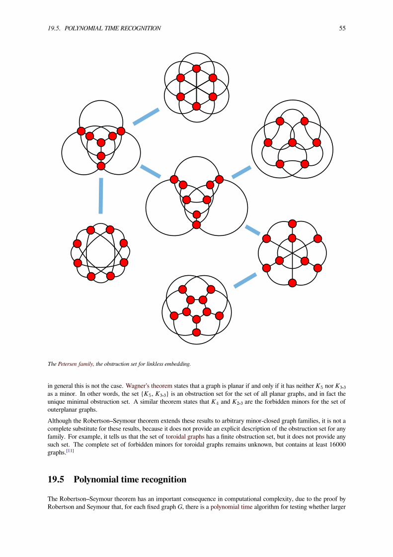
19.5. POLYNOMIAL TIME RECOGNITION 55

The Petersen family, the obstruction set for linkless embedding.

in general this is not the case. Wagner’s theorem states that a graph is planar if and only if it has neither K5 nor K₃,₃as a minor. In other words, the set {K5, K₃,₃} is an obstruction set for the set of all planar graphs, and in fact theunique minimal obstruction set. A similar theorem states that K4 and K₂,₃ are the forbidden minors for the set ofouterplanar graphs.Although the Robertson–Seymour theorem extends these results to arbitrary minor-closed graph families, it is not acomplete substitute for these results, because it does not provide an explicit description of the obstruction set for anyfamily. For example, it tells us that the set of toroidal graphs has a finite obstruction set, but it does not provide anysuch set. The complete set of forbidden minors for toroidal graphs remains unknown, but contains at least 16000graphs.[11]

19.5 Polynomial time recognition

The Robertson–Seymour theorem has an important consequence in computational complexity, due to the proof byRobertson and Seymour that, for each fixed graph G, there is a polynomial time algorithm for testing whether larger

56 CHAPTER 19. ROBERTSON–SEYMOUR THEOREM

graphs have G as a minor. The running time of this algorithm can be expressed as a cubic polynomial in the size ofthe larger graph (although there is a constant factor in this polynomial that depends superpolynomially on the size ofG), which has been improved to quadratic time by Kawarabayashi, Kobayashi, and Reed.[12] As a result, for everyminor-closed family F, there is polynomial time algorithm for testing whether a graph belongs to F: simply check,for each of the forbidden minors for F, whether the given graph contains that forbidden minor.[13]

However, this method requires a specific finite obstruction set to work, and the theorem does not provide one. Thetheorem proves that such a finite obstruction set exists, and therefore the problem is polynomial because of theabove algorithm. However, the algorithm can be used in practice only if such a finite obstruction set is provided.As a result, the theorem proves that the problem can be solved in polynomial time, but does not provide a concretepolynomial-time algorithm for solving it. Such proofs of polynomiality are non-constructive: they prove polynomialityof problems without providing an explicit polynomial-time algorithm.[14] In many specific cases, checking whether agraph is in a given minor-closed family can be done more efficiently: for example, checking whether a graph is planarcan be done in linear time.

19.6 Fixed-parameter tractability

For graph invariants with the property that, for each k, the graphs with invariant at most k are minor-closed, the samemethod applies. For instance, by this result, treewidth, branchwidth, and pathwidth, vertex cover, and the minimumgenus of an embedding are all amenable to this approach, and for any fixed k there is a polynomial time algorithm fortesting whether these invariants are at most k, in which the exponent in the running time of the algorithm does notdepend on k. A problem with this property, that it can be solved in polynomial time for any fixed k with an exponentthat does not depend on k, is known as fixed-parameter tractable.However, this method does not directly provide a single fixed-parameter-tractable algorithm for computing the pa-rameter value for a given graph with unknown k, because of the difficulty of determining the set of forbidden minors.Additionally, the large constant factors involved in these results make them highly impractical. Therefore, the devel-opment of explicit fixed-parameter algorithms for these problems, with improved dependence on k, has continued tobe an important line of research.

19.7 Finite form of the graph minor theorem

Friedman, Robertson & Seymour (1987) showed that the following theorem exhibits the independence phenomenonby being unprovable in various formal systems that are much stronger than Peano arithmetic, yet being provable insystems much weaker than ZFC:

Theorem: For every positive integer n, there is an integer m so large that if G1, ..., Gm is a sequence offinite undirected graphs,where each Gi has size at most n+i, then Gj ≤ Gk for some j < k.

(Here, the size of a graph is the total number of its nodes and edges, and ≤ denotes the minor ordering.)

19.8 See also

• Graph structure theorem

19.9 Notes[1] Bienstock & Langston (1995).

[2] Robertson & Seymour (2004).

[3] Robertson and Seymour (1983, 2004); Diestel (2005, p. 333).

19.10. REFERENCES 57

[4] Diestel (2005, p. 355).

[5] Diestel (2005, pp. 335–336); Lovász (2005), Section 3.3, pp. 78–79.

[6] E.g., see Bienstock & Langston (1995), Section 2, “well-quasi-orders”.

[7] Diestel (2005, p. 334).

[8] Lovász (2005, p. 78).

[9] Bienstock & Langston (1995), Corollary 2.1.1; Lovász (2005), Theorem 4, p. 78.

[10] Lovász (2005, pp. 76–77).

[11] Chambers (2002).

[12] Kawarabayashi, Kobayashi & Reed (2012)

[13] Robertson & Seymour (1995); Bienstock & Langston (1995), Theorem 2.1.4 and Corollary 2.1.5; Lovász (2005), Theorem11, p. 83.

[14] Fellows & Langston (1988); Bienstock & Langston (1995), Section 6.

19.10 References• Bienstock, Daniel; Langston, Michael A. (1995), “Algorithmic implications of the graph minor theorem”,NetworkModels (PDF), Handbooks inOperations Research andManagement Science 7, pp. 481–502, doi:10.1016/S0927-0507(05)80125-2.

• Chambers, J. (2002), Hunting for torus obstructions, M.Sc. thesis, Department of Computer Science, Univer-sity of Victoria.

• Diestel, Reinhard (2005), “Minors, Trees, and WQO”, Graph Theory (PDF) (Electronic Edition 2005 ed.),Springer, pp. 326–367.

• Fellows, Michael R.; Langston, Michael A. (1988), “Nonconstructive tools for proving polynomial-time decid-ability”, Journal of the ACM 35 (3): 727–739, doi:10.1145/44483.44491.

• Friedman, Harvey; Robertson, Neil; Seymour, Paul (1987), “The metamathematics of the graph minor the-orem”, in Simpson, S., Logic and Combinatorics, Contemporary Mathematics 65, American MathematicalSociety, pp. 229–261.

• Kawarabayashi, Ken-ichi; Kobayashi, Yusuke; Reed, Bruce (2012), “The disjoint paths problem in quadratictime” (PDF), Journal of Combinatorial Theory, Series B 102 (2): 424–435, doi:10.1016/j.jctb.2011.07.004.

• Lovász, László (2005), “Graph Minor Theory”, Bulletin of the American Mathematical Society (New Series) 43(1): 75–86, doi:10.1090/S0273-0979-05-01088-8.

• Robertson, Neil; Seymour, Paul (1983), “Graph Minors. I. Excluding a forest”, Journal of CombinatorialTheory, Series B 35 (1): 39–61, doi:10.1016/0095-8956(83)90079-5.

• Robertson, Neil; Seymour, Paul (1995), “Graph Minors. XIII. The disjoint paths problem”, Journal of Com-binatorial Theory, Series B 63 (1): 65–110, doi:10.1006/jctb.1995.1006.

• Robertson, Neil; Seymour, Paul (2004), “Graph Minors. XX. Wagner’s conjecture”, Journal of CombinatorialTheory, Series B 92 (2): 325–357, doi:10.1016/j.jctb.2004.08.001.

19.11 External links• Weisstein, Eric W., “Robertson-Seymour Theorem”, MathWorld.

Chapter 20

Scott–Potter set theory

An approach to the foundations of mathematics that is of relatively recent origin, Scott–Potter set theory is a col-lection of nested axiomatic set theories set out by the philosopher Michael Potter, building on earlier work by themathematician Dana Scott and the philosopher George Boolos.Potter (1990, 2004) clarified and simplified the approach of Scott (1974), and showed how the resulting axiomatic settheory can do what is expected of such theory, namely grounding the cardinal and ordinal numbers, Peano arithmeticand the other usual number systems, and the theory of relations.

20.1 ZU etc.

20.1.1 Preliminaries

This section and the next follow Part I of Potter (2004) closely. The background logic is first-order logic with identity.The ontology includes urelements as well as sets, which makes it clear that there can be sets of entities defined byfirst-order theories not based on sets. The urelements are not essential in that other mathematical structures can bedefined as sets, and it is permissible for the set of urelements to be empty.Some terminology peculiar to Potter’s set theory:

• ι is a definite description operator and binds a variable. (In Potter’s notation the iota symbol is inverted.)

• The predicate U holds for all urelements (non-collections).

• ιxΦ(x) exists iff (∃!x)Φ(x). (Potter uses Φ and other upper-case Greek letters to represent formulas.)

• {x : Φ(x)} is an abbreviation for ιy(not U(y) and (∀x)(x ∈ y ⇔ Φ(x))).

• a is a collection if {x : x∈a} exists. (All sets are collections, but not all collections are sets.)

• The accumulation of a, acc(a), is the set {x : x is a urelement or ∃b∈a (x∈b or x⊂b)}.

• If ∀v∈V(v = acc(V∩v)) then V is a history.

• A level is the accumulation of a history.

• An initial level has no other levels as members.

• A limit level is a level that is neither the initial level nor the level above any other level.

• A set is a subcollection of some level.

• The birthday of set a, denoted V(a), is the lowest level V such that a⊂V.

58

20.1. ZU ETC. 59

20.1.2 Axioms

The following three axioms define the theory ZU.Creation: ∀V∃V' (V∈V' ).Remark: There is no highest level, hence there are infinitely many levels. This axiom establishes the ontology oflevels.Separation: An axiom schema. For any first-order formula Φ(x) with (bound) variables ranging over the level V, thecollection {x∈V : Φ(x)} is also a set. (See Axiom schema of separation.)Remark: Given the levels established by Creation, this schema establishes the existence of sets and how to form them.It tells us that a level is a set, and all subsets, definable via first-order logic, of levels are also sets. This schema canbe seen as an extension of the background logic.Infinity: There exists at least one limit level. (See Axiom of infinity.)Remark: Among the sets Separation allows, at least one is infinite. This axiom is primarily mathematical, as thereis no need for the actual infinite in other human contexts, the human sensory order being necessarily finite. Formathematical purposes, the axiom “There exists an inductive set" would suffice.

20.1.3 Further existence premises

The following statements, while in the nature of axioms, are not axioms of ZU. Instead, they assert the existence ofsets satisfying a stated condition. As such, they are “existence premises,” meaning the following. Let X denote anystatement below. Any theorem whose proof requiresX is then formulated conditionally as “If X holds, then...” Potterdefines several systems using existence premises, including the following two:

• ZfU = ZU + Ordinals;

• ZFU = Separation + Reflection.

Ordinals: For each (infinite) ordinal α, there exists a corresponding level Vα.Remark: In words, “There exists a level corresponding to each infinite ordinal.” Ordinals makes possible the conven-tional Von Neumann definition of ordinal numbers.Let τ(x) be a first-order term.Replacement: An axiom schema. For any collection a, ∀x∈a[τ(x) is a set] → {τ(x) : x∈a} is a set.Remark: If the term τ(x) is a function (call it f(x)), and if the domain of f is a set, then the range of f is also a set.Reflection: Let Φ denote a first-order formula in which any number of free variables are present. Let Φ(V) denote Φwith these free variables all quantified, with the quantified variables restricted to the level V.Then ∃V[Φ→Φ(V)] is an axiom.Remark: This schema asserts the existence of a “partial” universe, namely the levelV, in which all properties Φ holdingwhen the quantified variables range over all levels, also hold when these variables range over V only. Reflection turnsCreation, Infinity, Ordinals, and Replacement into theorems (Potter 2004: §13.3).Let A and a denote sequences of nonempty sets, each indexed by n.Countable Choice: Given any sequence A, there exists a sequence a such that:

∀n∈ω[a ∈A ].

Remark. Countable Choice enables proving that any set must be one of finite or infinite.Let B and C denote sets, and let n index the members of B, each denoted Bn.Choice: Let the members of B be disjoint nonempty sets. Then:

∃C∀n[C∩Bn is a singleton].

60 CHAPTER 20. SCOTT–POTTER SET THEORY

20.2 Discussion

The Von Neumann universe implements the “iterative conception of set” by stratifying the universe of sets into aseries of “levels,” with the sets at a given level being the members of the sets making up the next higher level. Hencethe levels form a nested and well-ordered sequence, and would form a hierarchy if set membership were transitive.The resulting iterative conception steers clear, in a well-motivated way, of the well-known paradoxes of Russell,Burali-Forti, and Cantor. These paradoxes all result from the unrestricted use of the principle of comprehension thatnaive set theory allows. Collections such as “the class of all sets” or “the class of all ordinals” include sets from alllevels of the hierarchy. Given the iterative conception, such collections cannot form sets at any given level of thehierarchy and thus cannot be sets at all. The iterative conception has gradually become more accepted over time,despite an imperfect understanding of its historical origins.Boolos’s (1989) axiomatic treatment of the iterative conception is his set theory S, a two sorted first order theoryinvolving sets and levels.

20.2.1 Scott’s theory

Scott (1974) did not mention the “iterative conception of set,” instead proposing his theory as a natural outgrowth ofthe simple theory of types. Nevertheless, Scott’s theory can be seen as an axiomatization of the iterative conceptionand the associated iterative hierarchy.Scott began with an axiom he declined to name: the atomic formula x∈y implies that y is a set. In symbols:

∀x,y∃a[x∈y→y=a].

His axiom of Extensionality and axiom schema of Comprehension (Separation) are strictly analogous to their ZFcounterparts and so do not mention levels. He then invoked two axioms that do mention levels:

• Accumulation. A given level “accumulates” all members and subsets of all earlier levels. See the above definitionof accumulation.

• Restriction. All collections belong to some level.

Restriction also implies the existence of at least one level and assures that all sets are well-founded.Scott’s final axiom, the Reflection schema, is identical to the above existence premise bearing the same name, andlikewise does duty for ZF’s Infinity and Replacement. Scott’s system has the same strength as ZF.

20.2.2 Potter’s theory

Potter (1990, 2004) introduced the idiosyncratic terminology described earlier in this entry, and discarded or replacedall of Scott’s axioms except Reflection; the result is ZU. ZU, like ZF, cannot be finitely axiomatized. ZU differs fromZFC in that it:

• Includes no axiom of extensionality because the usual extensionality principle follows from the definition ofcollection and an easy lemma.

• Admits nonwellfounded collections. However Potter (2004) never invokes such collections, and all sets (col-lections which are contained in a level) are wellfounded. No theorem in Potter would be overturned if an axiomstating that all collections are sets were added to ZU.

• Includes no equivalents of Choice or the axiom schema of Replacement.

Hence ZU is closer to the Zermelo set theory of 1908, namely ZFC minus Choice, Replacement, and Foundation.It is stronger than this theory, however, since cardinals and ordinals can be defined, despite the absence of Choice,using Scott’s trick and the existence of levels, and no such definition is possible in Zermelo set theory. Thus in ZU,an equivalence class of:

20.3. SEE ALSO 61

• Equinumerous sets from a common level is a cardinal number;

• Isomorphic well-orderings, also from a common level, is an ordinal number.

Similarly the natural numbers are not defined as a particular set within the iterative hierarchy, but as models of a“pure” Dedekind algebra. “Dedekind algebra” is Potter’s name for a set closed under a unary injective operation,successor, whose domain contains a unique element, zero, absent from its range. Because the theory of Dedekindalgebras is categorical (all models are isomorphic), any such algebra can proxy for the natural numbers.Although Potter (2004) devotes an entire appendix to proper classes, the strength and merits of Scott–Potter settheory relative to the well-known rivals to ZFC that admit proper classes, namely NBG and Morse–Kelley set theory,have yet to be explored.Scott–Potter set theory resembles NFU in that the latter is a recently (Jensen 1967) devised axiomatic set theoryadmitting both urelements and sets that are not well-founded. But the urelements of NFU, unlike those of ZU, play anessential role; they and the resulting restrictions on Extensionality make possible a proof of NFU’s consistency relativeto Peano arithmetic. But nothing is known about the strength of NFU relative to Creation+Separation, NFU+Infinityrelative to ZU, and of NFU+Infinity+Countable Choice relative to ZU + Countable Choice.Unlike nearly all writing on set theory in recent decades, Potter (2004) mentions mereological fusions. His collectionsare also synonymous with the “virtual sets” of Willard Quine and Richard Milton Martin: entities arising from thefree use of the principle of comprehension that can never be admitted to the universe of discourse.

20.3 See also

• Foundation of mathematics

• Hierarchy (mathematics)

• List of set theory topics

• Philosophy of mathematics

• S (Boolos 1989)

• Von Neumann universe

• Zermelo set theory

• ZFC

20.4 References

• George Boolos, 1971, “The iterative conception of set,” Journal of Philosophy 68: 215–31. Reprinted inBoolos 1999. Logic, Logic, and Logic. Harvard Univ. Press: 13-29.

• --------, 1989, “Iteration Again,” Philosophical Topics 42: 5-21. Reprinted in Boolos 1999. Logic, Logic, andLogic. Harvard Univ. Press: 88-104.

• Potter, Michael, 1990. Sets: An Introduction. Oxford Univ. Press.

• ------, 2004. Set Theory and its Philosophy. Oxford Univ. Press.

• Dana Scott, 1974, “Axiomatizing set theory” in Jech, Thomas, J., ed., Axiomatic Set Theory II, Proceedings ofSymposia in Pure Mathematics 13. American Mathematical Society: 207–14.

62 CHAPTER 20. SCOTT–POTTER SET THEORY

20.5 External links

Reviews of Potter (2004):

• Bays, Timothy, 2005, "Review," Notre Dame Philosophical Reviews.

• Uzquiano, Gabriel, 2005, "Review," Philosophia Mathematica 13: 308-46.

Chapter 21

Structural induction

Structural induction is a proof method that is used in mathematical logic (e.g., in the proof of Łoś' theorem),computer science, graph theory, and some other mathematical fields. It is a generalization of mathematical inductionover natural numbers, and can be further generalized to arbitrary Noetherian induction. Structural recursion isa recursion method bearing the same relationship to structural induction as ordinary recursion bears to ordinarymathematical induction.Structural induction is used to prove that some proposition P(x) holds for all x of some sort of recursively definedstructure such as lists or trees. A well-founded partial order is defined on the structures (“sublist” for lists and “subtree”for trees). The structural induction proof is a proof that the proposition holds for all the minimal structures, and thatif it holds for the immediate substructures of a certain structure S, then it must hold for S also. (Formally speaking,this then satisfies the premises of an axiom of well-founded induction, which asserts that these two conditions aresufficient for the proposition to hold for all x.)A structurally recursive function uses the same idea to define a recursive function: “base cases” handle each minimalstructure and a rule for recursion. Structural recursion is usually proved correct by structural induction; in particularlyeasy cases, the inductive step is often left out. The length and ++ functions in the example below are structurallyrecursive.For example, if the structures are lists, one usually introduces the partial order '<' in which L < M whenever list L isthe tail of listM. Under this ordering, the empty list [] is the unique minimal element. A structural induction proof ofsome proposition P(l) then consists of two parts: A proof that P([]) is true, and a proof that if P(L) is true for somelist L, and if L is the tail of list M, then P(M) must also be true.Eventually, there may exist more than one base case, and/or more than one inductive case, depending on how thefunction or structure was constructed. In those cases, a structural induction proof of some proposition P(l) thenconsists of: A) a proof that P(BC) is true for each base case BC, and B): a proof that if P(I) is true for some instanceI, and M can be obtained from I by applying any one recursive rule once, then P(M) must also be true.

21.1 Examples

An ancestor tree is a commonly known data structure, showing the parents, grandparents, etc. of a person as far asknown (see picture for an example). It is recursively defined:

• in the simplest case, an ancestor tree shows just one person (if nothing is known about his/her parents);

• alternatively, an ancestor tree shows one person and, connected by branches, the two ancestor subtrees ofhis/her parents (using for brevity of proof the simplifying assumption that if one of them is known, both are).

As an example, the property “An ancestor tree extending over g generations shows at most 2g−1 persons” can beproven by structural induction as follows:

• In the simplest case, the tree shows just one person and hence one generation; the property is true for such atree, since 1 ≤ 21−1.

63

64 CHAPTER 21. STRUCTURAL INDUCTION

Ancient ancestor tree, showing 31 persons in 5 generations.

• Alternatively, the tree shows one person and his/her parents’ trees. Since each of the latter is a substructure ofthe whole tree, it can be assumed to satisfy the property to be proven (a.k.a. the induction hypothesis). That is,p ≤ 2g−1 and q ≤ 2h−1 can be assumed, where g and h denotes the number of generations the father’s and themother’s subtree extends over, respectively, and p and q denote the numbers of persons they show.

• In case g≤ h, the whole tree extends over 1+h generations and shows p+q+1 persons, and p+q+1 ≤ (2g−1)+ (2h−1) + 1 ≤ 2h + 2h - 1 = 21+h - 1, i.e. the whole tree satisfies the property.

• In case h ≤ g, the whole tree extends over 1+g generations and shows p+q+1 ≤ 21+g - 1 persons by similarreasoning, i.e. the whole tree satisfies the property in this case also.

Hence, by structural induction, each ancestor tree satisfies the property.As another, more formal example, consider the following property of lists:length (L ++ M) = length L + length M [EQ]Here ++ denotes the list concatenation operation, and L and M are lists.In order to prove this, we need definitions for length and for the concatenation operation. Let (h:t) denote a list whosehead (first element) is h and whose tail (list of remaining elements) is t, and let [] denote the empty list. The definitionsfor length and the concatenation operation are:length [] = 0 [LEN1] length (h:t) = 1 + length t [LEN2] [] ++ list = list [APP1] (h:t) ++ list = h : (t ++ list) [APP2]Our proposition P(l) is that EQ is true for all lists M when L is l. We want to show that P(l) is true for all lists l. Wewill prove this by structural induction on lists.First we will prove that P([]) is true; that is, EQ is true for all listsM when L happens to be the empty list []. ConsiderEQ:length (L ++M) = length ([] ++ M) = length M (by APP1) = 0 + length M = length [] + length M (by LEN1) = lengthL + length M

21.2. WELL-ORDERING 65

So this part of the theorem is proved; EQ is true for allM, when L is [], because the left-hand side and the right-handside are equal.Next, consider any nonempty list I. Since I is nonempty, it has a head item, x, and a tail list, xs, so we can express itas (x:xs). The induction hypothesis is that EQ is true for all values of M when L is xs:length (xs ++ M) = length xs + length M (hypothesis)We would like to show that if this is the case, then EQ is also true for all values ofM when L = I = (x:xs). We proceedas before:length L + length M = length (x:xs) + length M = 1 + length xs + length M (by LEN2) = 1 + length (xs ++ M) (byhypothesis) = length (x: (xs ++ M)) (by LEN2) = length ((x:xs) ++ M) (by APP2) = length (L ++ M)Thus, from structural induction, we obtain that P(L) is true for all lists L.

21.2 Well-ordering

Just as standard mathematical induction is equivalent to the well-ordering principle, structural induction is also equiv-alent to a well-ordering principle. If the set of all structures of a certain kind admits a well-founded partial order, thenevery nonempty subset must have a minimal element. (This is the definition of "well-founded".) The significance ofthe lemma in this context is that it allows us to deduce that if there are any counterexamples to the theorem we wantto prove, then there must be a minimal counterexample. If we can show the existence of the minimal counterexampleimplies an even smaller counterexample, we have a contradiction (since the minimal counterexample isn't minimal)and so the set of counterexamples must be empty.As an example of this type of argument, consider the set of all binary trees. We will show that the number of leavesin a full binary tree is one more than the number of interior nodes. Suppose there is a counterexample; then theremust exist one with the minimal possible number of interior nodes. This counterexample, C, has n interior nodes andl leaves, where n+1 ≠ l. Moreover, C must be nontrivial, because the trivial tree has n = 0 and l = 1 and is thereforenot a counterexample. C therefore has at least one leaf whose parent node is an interior node. Delete this leaf and itsparent from the tree, promoting the leaf’s sibling node to the position formerly occupied by its parent. This reducesboth n and l by 1, so the new tree also has n+1 ≠ l and is therefore a smaller counterexample. But by hypothesis,C was already the smallest counterexample; therefore, the supposition that there were any counterexamples to beginwith must have been false. The partial ordering implied by 'smaller' here is the one that says that S < T whenever Shas fewer nodes than T.

21.3 See also• Coinduction

• Initial algebra

21.4 References• Hopcroft, John E.; Rajeev Motwani; Jeffrey D. Ullman (2001). Introduction to Automata Theory, Languages,and Computation (2nd ed.). Reading Mass: Addison-Wesley. ISBN 0-201-44124-1.

Early publications about structural induction include:

• Burstall, R.M. (1969). “Proving Properties of Programs by Structural Induction”. The Computer Journal 12(1): 41–48. doi:10.1093/comjnl/12.1.41.

• Aubin, Raymond (1976), Mechanizing Structural Induction, EDI-INF-PHD, 76-002, University of Edinburgh

• Huet, G.; Hullot, J.M. (1980). “Proofs by Induction in Equational Theories with Constructors”. 21st Ann.Symp. on Foundations of Computer Science. IEEE. pp. 96–107.

Chapter 22

Universal set

For other uses, see Universal set (disambiguation).

In set theory, a universal set is a set which contains all objects, including itself.[1] In set theory as usually formulated,the conception of a universal set leads to a paradox (Russell’s paradox) and is consequently not allowed. However,some non-standard variants of set theory include a universal set. It is often symbolized by the Greek letter xi.

22.1 Reasons for nonexistence

Zermelo–Fraenkel set theory and related set theories, which are based on the idea of the cumulative hierarchy, donot allow for the existence of a universal set. Its existence would cause paradoxes which would make the theoryinconsistent.

22.1.1 Russell’s paradox

Russell’s paradox prevents the existence of a universal set in Zermelo–Fraenkel set theory and other set theories thatinclude Zermelo's axiom of comprehension. This axiom states that, for any formula φ(x) and any set A, there existsanother set

{x ∈ A | φ(x)}

that contains exactly those elements x of A that satisfyφ . If a universal set V existed and the axiom of comprehensioncould be applied to it, then there would also exist another set {x ∈ V | x ̸∈ x} , the set of all sets that do not containthemselves. However, as Bertrand Russell observed, this set is paradoxical. If it contains itself, then it should notcontain itself, and vice versa. For this reason, it cannot exist.

22.1.2 Cantor’s theorem

A second difficulty with the idea of a universal set concerns the power set of the set of all sets. Because this power setis a set of sets, it would automatically be a subset of the set of all sets, provided that both exist. However, this conflictswith Cantor’s theorem that the power set of any set (whether infinite or not) always has strictly higher cardinality thanthe set itself.

22.2 Theories of universality

The difficulties associated with a universal set can be avoided either by using a variant of set theory in which theaxiom of comprehension is restricted in some way, or by using a universal object that is not considered to be a set.

66

22.3. NOTES 67

22.2.1 Restricted comprehension

There are set theories known to be consistent (if the usual set theory is consistent) in which the universal set V doesexist (and V ∈ V is true). In these theories, Zermelo’s axiom of comprehension does not hold in general, and theaxiom of comprehension of naive set theory is restricted in a different way. A set theory containing a universal set isnecessarily a non-well-founded set theory.The most widely studied set theory with a universal set is Willard Van Orman Quine’s New Foundations. AlonzoChurch and Arnold Oberschelp also published work on such set theories. Church speculated that his theory mightbe extended in a manner consistent with Quine’s,[2] but this is not possible for Oberschelp’s, since in it the singletonfunction is provably a set,[3] which leads immediately to paradox in New Foundations.[4] The most recent advancesin this area have been made by Randall Holmes who published an online draft version of the book Elementary SetTheory with a Universal Set in 2012.[5]

22.2.2 Universal objects that are not sets

Main article: Universe (mathematics)

The idea of a universal set seems intuitively desirable in the Zermelo–Fraenkel set theory, particularly because mostversions of this theory do allow the use of quantifiers over all sets (see universal quantifier). One way of allowingan object that behaves similarly to a universal set, without creating paradoxes, is to describe V and similar largecollections as proper classes rather than as sets. One difference between a universal set and a universal class is thatthe universal class does not contain itself, because proper classes cannot be elements of other classes. Russell’sparadox does not apply in these theories because the axiom of comprehension operates on sets, not on classes.The category of sets can also be considered to be a universal object that is, again, not itself a set. It has all sets aselements, and also includes arrows for all functions from one set to another. Again, it does not contain itself, becauseit is not itself a set.

22.3 Notes[1] Forster 1995 p. 1.

[2] Church 1974 p. 308. See also Forster 1995 p. 136 or 2001 p. 17.

[3] Oberschelp 1973 p. 40.

[4] Holmes 1998 p. 110.

[5] http://math.boisestate.edu/~{}holmes/

22.4 References• Alonzo Church (1974). “Set Theory with a Universal Set,” Proceedings of the Tarski Symposium. Proceedingsof Symposia in Pure Mathematics XXV, ed. L. Henkin, American Mathematical Society, pp. 297–308.

• T. E. Forster (1995). Set Theory with a Universal Set: Exploring an Untyped Universe (Oxford Logic Guides31). Oxford University Press. ISBN 0-19-851477-8.

• T. E. Forster (2001). “Church’s Set Theory with a Universal Set.”• Bibliography: Set Theory with a Universal Set, originated by T. E. Forster and maintained by Randall Holmesat Boise State University.

• Randall Holmes (1998). Elementary Set theory with a Universal Set, volume 10 of the Cahiers du Centre deLogique, Academia, Louvain-la-Neuve (Belgium).

• Arnold Oberschelp (1973). “Set Theory over Classes,” Dissertationes Mathematicae 106.• WillardVanOrmanQuine (1937) “NewFoundations forMathematical Logic,”AmericanMathematicalMonthly44, pp. 70–80.

68 CHAPTER 22. UNIVERSAL SET

22.5 External links• Weisstein, Eric W., “Universal Set”, MathWorld.

Chapter 23

Well-founded relation

“Noetherian induction” redirects here. For the use in topology, see Noetherian topological space.

In mathematics, a binary relation, R, is well-founded (or wellfounded) on a class X if and only if every non-emptysubset S X has a minimal element; that is, some element m of any S is not related by sRm (for instance, "m is notsmaller than”) for the rest of the s ∈ S.

∀S ⊆ X (S ̸= ∅ → ∃m ∈ S ∀s ∈ S (s,m) /∈ R)

(Some authors include an extra condition that R is set-like, i.e., that the elements less than any given element form aset.)Equivalently, assuming some choice, a relation is well-founded if and only if it contains no countable infinite descend-ing chains: that is, there is no infinite sequence x0, x1, x2, ... of elements of X such that xn₊₁ R x for every naturalnumber n.In order theory, a partial order is called well-founded if the corresponding strict order is a well-founded relation. Ifthe order is a total order then it is called a well-order.In set theory, a set x is called a well-founded set if the set membership relation is well-founded on the transitiveclosure of x. The axiom of regularity, which is one of the axioms of Zermelo–Fraenkel set theory, asserts that all setsare well-founded.A relation R is converse well-founded, upwards well-founded or Noetherian on X, if the converse relation R−1is well-founded on X. In this case R is also said to satisfy the ascending chain condition. In the context of rewritingsystems, a Noetherian relation is also called terminating.

23.1 Induction and recursion

An important reason that well-founded relations are interesting is because a version of transfinite induction can beused on them: if (X, R) is a well-founded relation, P(x) is some property of elements of X, and we want to show that

P(x) holds for all elements x of X,

it suffices to show that:

If x is an element of X and P(y) is true for all y such that y R x, then P(x) must also be true.

That is,

∀x ∈ X [(∀y ∈ X (y Rx → P (y))) → P (x)] → ∀x ∈ X P (x).

69

70 CHAPTER 23. WELL-FOUNDED RELATION

Well-founded induction is sometimes called Noetherian induction,[1] after Emmy Noether.On par with induction, well-founded relations also support construction of objects by transfinite recursion. Let (X,R) be a set-like well-founded relation and F a function that assigns an object F(x, g) to each pair of an element x ∈ Xand a function g on the initial segment {y: y R x} of X. Then there is a unique function G such that for every x ∈ X,

G(x) = F (x,G|{y:y Rx})

That is, if we want to construct a function G on X, we may define G(x) using the values of G(y) for y R x.As an example, consider the well-founded relation (N, S), whereN is the set of all natural numbers, and S is the graphof the successor function x → x + 1. Then induction on S is the usual mathematical induction, and recursion on Sgives primitive recursion. If we consider the order relation (N, <), we obtain complete induction, and course-of-valuesrecursion. The statement that (N, <) is well-founded is also known as the well-ordering principle.There are other interesting special cases of well-founded induction. When the well-founded relation is the usualordering on the class of all ordinal numbers, the technique is called transfinite induction. When the well-founded setis a set of recursively-defined data structures, the technique is called structural induction. When the well-foundedrelation is set membership on the universal class, the technique is known as ∈-induction. See those articles for moredetails.

23.2 Examples

Well-founded relations which are not totally ordered include:

• the positive integers {1, 2, 3, ...}, with the order defined by a < b if and only if a divides b and a ≠ b.

• the set of all finite strings over a fixed alphabet, with the order defined by s < t if and only if s is a propersubstring of t.

• the set N × N of pairs of natural numbers, ordered by (n1, n2) < (m1, m2) if and only if n1 < m1 and n2 < m2.

• the set of all regular expressions over a fixed alphabet, with the order defined by s < t if and only if s is a propersubexpression of t.

• any class whose elements are sets, with the relation ∈ (“is an element of”). This is the axiom of regularity.

• the nodes of any finite directed acyclic graph, with the relation R defined such that a R b if and only if there isan edge from a to b.

Examples of relations that are not well-founded include:

• the negative integers {−1,−2,−3, …}, with the usual order, since any unbounded subset has no least element.

• The set of strings over a finite alphabet with more than one element, under the usual (lexicographic) order,since the sequence “B” > “AB” > “AAB” > “AAAB” > … is an infinite descending chain. This relation failsto be well-founded even though the entire set has a minimum element, namely the empty string.

• the rational numbers (or reals) under the standard ordering, since, for example, the set of positive rationals (orreals) lacks a minimum.

23.3 Other properties

If (X, <) is a well-founded relation and x is an element of X, then the descending chains starting at x are all finite, butthis does not mean that their lengths are necessarily bounded. Consider the following example: Let X be the union ofthe positive integers and a new element ω, which is bigger than any integer. Then X is a well-founded set, but thereare descending chains starting at ω of arbitrary great (finite) length; the chain ω, n − 1, n − 2, ..., 2, 1 has length nfor any n.

23.4. REFLEXIVITY 71

The Mostowski collapse lemma implies that set membership is a universal among the extensional well-founded rela-tions: for any set-like well-founded relation R on a class X which is extensional, there exists a class C such that (X,R)is isomorphic to (C,∈).

23.4 Reflexivity

A relation R is said to be reflexive if a R a holds for every a in the domain of the relation. Every reflexive relation on anonempty domain has infinite descending chains, because any constant sequence is a descending chain. For example,in the natural numbers with their usual order ≤, we have 1 ≥ 1 ≥ 1 ≥ · · · . To avoid these trivial descendingsequences, when working with a reflexive relation R it is common to use (perhaps implicitly) the alternate relation R′defined such that a R′ b if and only if a R b and a ≠ b. In the context of the natural numbers, this means that therelation <, which is well-founded, is used instead of the relation ≤, which is not. In some texts, the definition of awell-founded relation is changed from the definition above to include this convention.

23.5 References[1] Bourbaki, N. (1972) Elements of mathematics. Commutative algebra, Addison-Wesley.

• Just, Winfried and Weese, Martin, Discovering Modern Set theory. I, American Mathematical Society (1998)ISBN 0-8218-0266-6.

Chapter 24

Well-order

In mathematics, a well-order relation (or well-ordering) on a set S is a total order on S with the property that everynon-empty subset of S has a least element in this ordering. The set S together with the well-order relation is thencalled awell-ordered set. The hyphen is frequently omitted in contemporary papers, yielding the spellingswellorder,wellordered, and wellordering.Every non-empty well-ordered set has a least element. Every element s of a well-ordered set, except a possible greatestelement, has a unique successor (next element), namely the least element of the subset of all elements greater thans. There may be elements besides the least element which have no predecessor (see Natural numbers below for anexample). In a well-ordered set S, every subset T which has an upper bound has a least upper bound, namely the leastelement of the subset of all upper bounds of T in S.If ≤ is a non-strict well-ordering, then < is a strict well-ordering. A relation is a strict well-ordering if and only if it isa well-founded strict total order. The distinction between strict and non-strict well-orders is often ignored since theyare easily interconvertible.Every well-ordered set is uniquely order isomorphic to a unique ordinal number, called the order type of the well-ordered set. The well-ordering theorem, which is equivalent to the axiom of choice, states that every set can bewell-ordered. If a set is well-ordered (or even if it merely admits a wellfounded relation), the proof technique oftransfinite induction can be used to prove that a given statement is true for all elements of the set.The observation that the natural numbers are well-ordered by the usual less-than relation is commonly called thewell-ordering principle (for natural numbers).

24.1 Ordinal numbers

Main article: Ordinal number

Every well-ordered set is uniquely order isomorphic to a unique ordinal number, called the order type of the well-ordered set. The position of each element within the ordered set is also given by an ordinal number. In the case of afinite set, the basic operation of counting, to find the ordinal number of a particular object, or to find the object witha particular ordinal number, corresponds to assigning ordinal numbers one by one to the objects. The size (numberof elements, cardinal number) of a finite set is equal to the order type. Counting in the everyday sense typically startsfrom one, so it assigns to each object the size of the initial segment with that object as last element. Note that thesenumbers are one more than the formal ordinal numbers according to the isomorphic order, because these are equalto the number of earlier objects (which corresponds to counting from zero). Thus for finite n, the expression "n-thelement” of a well-ordered set requires context to know whether this counts from zero or one. In a notation "β-thelement” where β can also be an infinite ordinal, it will typically count from zero.For an infinite set the order type determines the cardinality, but not conversely: well-ordered sets of a particularcardinality can have many different order types. For a countably infinite set, the set of possible order types is evenuncountable.

72

24.2. EXAMPLES AND COUNTEREXAMPLES 73

24.2 Examples and counterexamples

24.2.1 Natural numbers

The standard ordering ≤ of the natural numbers is a well-ordering and has the additional property that every non-zeronatural number has a unique predecessor.Another well-ordering of the natural numbers is given by defining that all even numbers are less than all odd numbers,and the usual ordering applies within the evens and the odds:

0 2 4 6 8 ... 1 3 5 7 9 ...

This is a well-ordered set of order type ω + ω. Every element has a successor (there is no largest element). Twoelements lack a predecessor: 0 and 1.

24.2.2 Integers

Unlike the standard ordering ≤ of the natural numbers, the standard ordering ≤ of the integers is not a well-ordering,since, for example, the set of negative integers does not contain a least element.The following relation R is an example of well-ordering of the integers: x R y if and only if one of the followingconditions holds:

1. x = 0

2. x is positive, and y is negative

3. x and y are both positive, and x ≤ y

4. x and y are both negative, and |x| ≤ |y|

This relation R can be visualized as follows:

0 1 2 3 4 ... −1 −2 −3 ...

R is isomorphic to the ordinal number ω + ω.Another relation for well-ordering the integers is the following definition: x ≤ y iff (|x| < |y| or (|x| = |y| and x ≤ y)).This well-order can be visualized as follows:

0 −1 1 −2 2 −3 3 −4 4 ...

This has the order type ω.

24.2.3 Reals

The standard ordering ≤ of any real interval is not a well-ordering, since, for example, the open interval (0, 1) ⊆ [0,1]does not contain a least element. From the ZFC axioms of set theory (including the axiom of choice) one can showthat there is a well-order of the reals. Also Wacław Sierpiński proved that ZF + GCH (the generalized continuumhypothesis) imply the axiom of choice and hence a well-order of the reals. Nonetheless, it is possible to show thatthe ZFC+GCH axioms alone are not sufficient to prove the existence of a definable (by a formula) well-order ofthe reals.[1] However it is consistent with ZFC that a definable well-ordering of the reals exists—for example, it isconsistent with ZFC that V=L, and it follows from ZFC+V=L that a particular formula well-orders the reals, or indeedany set.An uncountable subset of the real numbers with the standard ordering ≤ cannot be a well-order: SupposeX is a subsetof R well-ordered by ≤. For each x in X, let s(x) be the successor of x in ≤ ordering on X (unless x is the last elementof X). Let A = { (x, s(x)) | x ∈ X } whose elements are nonempty and disjoint intervals. Each such interval contains

74 CHAPTER 24. WELL-ORDER

at least one rational number, so there is an injective function from A to Q. There is an injection from X to A (exceptpossibly for a last element of X which could be mapped to zero later). And it is well known that there is an injectionfrom Q to the natural numbers (which could be chosen to avoid hitting zero). Thus there is an injection from X to thenatural numbers which means that X is countable. On the other hand, a countably infinite subset of the reals may ormay not be a well-order with the standard "≤".

• The natural numbers are a well-order.

• The set {1/n : n =1,2,3,...} has no least element and is therefore not a well-order (again, under standard ordering≤).

Examples of well-orders:

• The set of numbers { − 2−n | 0 ≤ n < ω } has order type ω.

• The set of numbers { − 2−n − 2−m−n | 0 ≤ m,n < ω } has order type ω². The previous set is the set of limitpoints within the set. Within the set of real numbers, either with the ordinary topology or the order topology,0 is also a limit point of the set. It is also a limit point of the set of limit points.

• The set of numbers { − 2−n | 0 ≤ n < ω } ∪ { 1 } has order type ω + 1. With the order topology of this set, 1 isa limit point of the set. With the ordinary topology (or equivalently, the order topology) of the real numbers itis not.

24.3 Equivalent formulations

If a set is totally ordered, then the following are equivalent to each other:

1. The set is well-ordered. That is, every nonempty subset has a least element.

2. Transfinite induction works for the entire ordered set.

3. Every strictly decreasing sequence of elements of the set must terminate after only finitelymany steps (assumingthe axiom of dependent choice).

4. Every subordering is isomorphic to an initial segment.

24.4 Order topology

Every well-ordered set can be made into a topological space by endowing it with the order topology.With respect to this topology there can be two kinds of elements:

• isolated points - these are the minimum and the elements with a predecessor.

• limit points - this type does not occur in finite sets, and may or may not occur in an infinite set; the infinite setswithout limit point are the sets of order type ω, for example N.

For subsets we can distinguish:

• Subsets with a maximum (that is, subsets which are bounded by themselves); this can be an isolated point or alimit point of the whole set; in the latter case it may or may not be also a limit point of the subset.

• Subsets which are unbounded by themselves but bounded in the whole set; they have no maximum, but asupremum outside the subset; if the subset is non-empty this supremum is a limit point of the subset and hencealso of the whole set; if the subset is empty this supremum is the minimum of the whole set.

• Subsets which are unbounded in the whole set.

24.5. SEE ALSO 75

A subset is cofinal in the whole set if and only if it is unbounded in the whole set or it has a maximum which is alsomaximum of the whole set.A well-ordered set as topological space is a first-countable space if and only if it has order type less than or equal toω1 (omega-one), that is, if and only if the set is countable or has the smallest uncountable order type.

24.5 See also• Tree (set theory), generalization

• Well-ordering theorem

• Ordinal number

• Well-founded set

• Well partial order

• Prewellordering

• Directed set

24.6 References[1] S. Feferman: “Some Applications of the Notions of Forcing and Generic Sets”, Fundamenta Mathematicae, 56 (1964)

325-345

• Folland, Gerald B. (1999). Real Analysis: Modern Techniques and Their Applications. Pure and applied math-ematics (2nd ed.). John Wiley & Sons. pp. 4–6, 9. ISBN 978-0-471-31716-6.

Chapter 25

Well-ordering principle

Not to be confused with Well-ordering theorem.

In mathematics, the well-ordering principle states that every non-empty set of positive integers contains a leastelement.[1] In other words, the set of positive integers is well-ordered.The phrase “well-ordering principle” is sometimes taken to be synonymous with the "well-ordering theorem". Onother occasions it is understood to be the proposition that the set of integers {…, −2, −1, 0, 1, 2, 3, …} contains awell-ordered subset, called the natural numbers, in which every nonempty subset contains a least element.Depending on the framework in which the natural numbers are introduced, this (second order) property of the set ofnatural numbers is either an axiom or a provable theorem. For example:

• In Peano Arithmetic, second-order arithmetic and related systems, and indeed in most (not necessarily for-mal) mathematical treatments of the well-ordering principle, the principle is derived from the principle ofmathematical induction, which is itself taken as basic.

• Considering the natural numbers as a subset of the real numbers, and assuming that we know already that thereal numbers are complete (again, either as an axiom or a theorem about the real number system), i.e., everybounded (from below) set has an infimum, then also every set A of natural numbers has an infimum, say a*.We can now find an integer n* such that a* lies in the half-open interval (n*−1, n*], and can then show that wemust have a* = n*, and n* in A.

• In axiomatic set theory, the natural numbers are defined as the smallest inductive set (i.e., set containing 0 andclosed under the successor operation). One can (even without invoking the regularity axiom) show that theset of all natural numbers n such that "{0, …, n} is well-ordered” is inductive, and must therefore contain allnatural numbers; from this property one can conclude that the set of all natural numbers is also well-ordered.

In the second sense, the phrase is used when that proposition is relied on for the purpose of justifying proofs that takethe following form: to prove that every natural number belongs to a specified set S, assume the contrary and infer theexistence of a (non-zero) smallest counterexample. Then show either that there must be a still smaller counterexampleor that the smallest counterexample is not a counter example, producing a contradiction. This mode of argument bearsthe same relation to proof by mathematical induction that “If not B then not A” (the style of modus tollens) bearsto “If A then B” (the style of modus ponens). It is known light-heartedly as the "minimal criminal" method and issimilar in its nature to Fermat’s method of "infinite descent".Garrett Birkhoff and Saunders Mac Lane wrote in A Survey of Modern Algebra that this property, like the least upperbound axiom for real numbers, is non-algebraic; i.e., it cannot be deduced from the algebraic properties of the integers(which form an ordered integral domain).

25.1 References[1] Apostol, Tom (1976). Introduction to Analytic Number Theory. New York: Springer-Verlag. p. 13. ISBN 0-387-90163-9.

76

Chapter 26

Well-quasi-ordering

In mathematics, specifically order theory, a well-quasi-ordering or wqo is a quasi-ordering that is well-founded,meaning that any infinite sequence of elements x0 , x1 , x2 , … from X contains an increasing pair xi ≤ xj withi < j .

26.1 Motivation

Well-founded induction can be used on any set with a well-founded relation, thus one is interested in when a quasi-order is well-founded. However the class of well-founded quasiorders is not closed under certain operations - thatis, when a quasi-order is used to obtain a new quasi-order on a set of structures derived from our original set, thisquasiorder is found to be not well-founded. By placing stronger restrictions on the original well-founded quasiorderingone can hope to ensure that our derived quasiorderings are still well-founded.An example of this is the power set operation. Given a quasiordering ≤ for a set X one can define a quasiorder ≤+

on X 's power set P (X) by setting A ≤+ B if and only if for each element of A one can find some element of Bwhich is larger than it under ≤ . One can show that this quasiordering on P (X) needn't be well-founded, but if onetakes the original quasi-ordering to be a well-quasi-ordering, then it is.

26.2 Formal definition

Awell-quasi-ordering on a setX is a quasi-ordering (i.e., a reflexive, transitive binary relation) such that any infinitesequence of elements x0 , x1 , x2 , … from X contains an increasing pair xi ≤ xj with i < j . The set X is said tobe well-quasi-ordered, or shortly wqo.A well partial order, or a wpo, is a wqo that is a proper ordering relation, i.e., it is antisymmetric.Among other ways of defining wqo’s, one is to say that they are quasi-orderings which do not contain infinite strictlydecreasing sequences (of the form x0 > x1 > x2 >…) nor infinite sequences of pairwise incomparable elements.Hence a quasi-order ( X ,≤) is wqo if and only if it is well-founded and has no infinite antichains.

26.3 Examples

• (N,≤) , the set of natural numbers with standard ordering, is a well partial order (in fact, a well-order). How-ever, (Z,≤) , the set of positive and negative integers, is not a well-quasi-order, because it is not well-founded.

• (N, |) , the set of natural numbers ordered by divisibility, is not a well partial order: the prime numbers are aninfinite antichain.

• (Nk,≤) , the set of vectors of k natural numbers (where k is finite) with component-wise ordering, is a wellpartial order (Dickson’s lemma). More generally, if (X,≤) is well-quasi-order, then (Xk,≤k) is also a well-quasi-order for all k .

77

78 CHAPTER 26. WELL-QUASI-ORDERING

• LetX be an arbitrary finite set with at least two elements. The setX∗ ofwords overX ordered lexicographically(as in a dictionary) isnot awell-quasi-order because it contains the infinite decreasing sequence b, ab, aab, aaab, . . .. Similarly,X∗ ordered by the prefix relation is not a well-quasi-order, because the previous sequence is an in-finite antichain of this partial order. However,X∗ ordered by the subsequence relation is a well partial order.[1](If X has only one element, these three partial orders are identical.)

• More generally, (X∗,≤) , the set of finite X -sequences ordered by embedding is a well-quasi-order if andonly if (X,≤) is a well-quasi-order (Higman’s lemma). Recall that one embeds a sequence u into a sequence vby finding a subsequence of v that has the same length as u and that dominates it term by term. When (X,=)is a finite unordered set, u ≤ v if and only if u is a subsequence of v .

• (Xω,≤) , the set of infinite sequences over a well-quasi-order (X,≤) , ordered by embedding, is not a well-quasi-order in general. That is, Higman’s lemma does not carry over to infinite sequences. Better-quasi-orderings have been introduced to generalize Higman’s lemma to sequences of arbitrary lengths.

• Embedding between finite trees with nodes labeled by elements of a wqo (X,≤) is a wqo (Kruskal’s treetheorem).

• Embedding between infinite trees with nodes labeled by elements of a wqo (X,≤) is a wqo (Nash-Williams'theorem).

• Embedding between countable scattered linear order types is a well-quasi-order (Laver's theorem).

• Embedding between countable boolean algebras is a well-quasi-order. This follows from Laver’s theorem anda theorem of Ketonen.

• Finite graphs ordered by a notion of embedding called "graphminor" is a well-quasi-order (Robertson–Seymourtheorem).

• Graphs of finite tree-depth ordered by the induced subgraph relation form a well-quasi-order,[2] as do thecographs ordered by induced subgraphs.[3]

26.4 Wqo’s versus well partial orders

In practice, the wqo’s one manipulates are quite often not orderings (see examples above), and the theory is technicallysmoother if we do not require antisymmetry, so it is built with wqo’s as the basic notion.Observe that a wpo is a wqo, and that a wqo gives rise to a wpo between equivalence classes induced by the kernelof the wqo. For example, if we order Z by divisibility, we end up with n ≡ m if and only if n = ±m , so that(Z, |) ≈ (N, |) .

26.5 Infinite increasing subsequences

If ( X , ≤) is wqo then every infinite sequence x0 , x1 , x2 , … contains an infinite increasing subsequence xn0 ≤xn1 ≤ xn2 ≤… (with n0 < n1 < n2 <…). Such a subsequence is sometimes called perfect. This can be proved bya Ramsey argument: given some sequence (xi)i , consider the set I of indexes i such that xi has no larger or equalxj to its right, i.e., with i < j . If I is infinite, then the I -extracted subsequence contradicts the assumption that Xis wqo. So I is finite, and any xn with n larger than any index in I can be used as the starting point of an infiniteincreasing subsequence.The existence of such infinite increasing subsequences is sometimes taken as a definition for well-quasi-ordering,leading to an equivalent notion.

26.6 Properties of wqos

• Given a quasiordering (X,≤) the quasiordering (P (X),≤+) defined byA ≤+ B ⇐⇒ ∀a ∈ A∃b ∈ B(a ≤b) is well-founded if and only if (X,≤) is a wqo.[4]

26.7. NOTES 79

• A quasiordering is a wqo if and only if the corresponding partial order (obtained by quotienting by x ∼ y ⇐⇒x ≤ y ∧ y ≤ x ) has no infinite descending sequences or antichains. (This can be proved using a Ramseyargument as above.)

• Given a well-quasi-ordering (X,≤) , any sequence of subsets S0 ⊆ S1 ⊆ ... ⊆ X such that ∀i ∈ N, ∀x, y ∈X,x ≤ y∧x ∈ Si ⇒ y ∈ Si eventually stabilises (meaning there is an indexn ∈ N such thatSn = Sn+1 = ...; subsets S ⊆ X with the property ∀x, y ∈ X,x ≤ y ∧ x ∈ S ⇒ y ∈ S are usually called upward-closed):assuming the contrary ∀i ∈ N∃j ∈ N, j > i, ∃x ∈ Sj \Si , a contradiction is reached by extracting an infinitenon-ascending subsequence.

• Given a well-quasi-ordering (X,≤) , any subset S ⊆ X which is upward-closed with respect to ≤ has a finitenumber of minimal elements w.r.t. ≤ , for otherwise the minimal elements of S would constitute an infiniteantichain.

26.7 Notes[1] Gasarch, W. (1998), “A survey of recursive combinatorics”, Handbook of Recursive Mathematics, Vol. 2, Stud. Logic

Found. Math. 139, Amsterdam: North-Holland, pp. 1041–1176, doi:10.1016/S0049-237X(98)80049-9, MR 1673598.See in particular page 1160.

[2] Nešetřil, Jaroslav; Ossona de Mendez, Patrice (2012), “Lemma 6.13”, Sparsity: Graphs, Structures, and Algorithms, Algo-rithms and Combinatorics 28, Heidelberg: Springer, p. 137, doi:10.1007/978-3-642-27875-4, ISBN 978-3-642-27874-7,MR 2920058.

[3] Damaschke, Peter (1990), “Induced subgraphs and well-quasi-ordering”, Journal of Graph Theory 14 (4): 427–435,doi:10.1002/jgt.3190140406, MR 1067237.

[4] Forster, Thomas (2003). “Better-quasi-orderings and coinduction”. Theoretical Computer Science 309 (1–3): 111–123.doi:10.1016/S0304-3975(03)00131-2.

26.8 References• Dickson, L. E. (1913). “Finiteness of the odd perfect and primitive abundant numbers with r distinct primefactors”. American Journal of Mathematics 35 (4): 413–422. doi:10.2307/2370405. JSTOR 2370405.

• Higman, G. (1952). “Ordering by divisibility in abstract algebras”. Proceedings of the London MathematicalSociety 2: 326–336. doi:10.1112/plms/s3-2.1.326.

• Kruskal, J. B. (1972). “The theory of well-quasi-ordering: A frequently discovered concept”. Journal ofCombinatorial Theory. Series A 13 (3): 297–305. doi:10.1016/0097-3165(72)90063-5.

• Ketonen, Jussi (1978). “The structure of countable Boolean algebras”. Annals of Mathematics 108 (1): 41–89.doi:10.2307/1970929. JSTOR 1970929.

• Milner, E. C. (1985). “Basic WQO- and BQO-theory”. In Rival, I. Graphs and Order. The Role of Graphs inthe Theory of Ordered Sets and Its Applications. D. Reidel Publishing Co. pp. 487–502. ISBN 90-277-1943-8.

• Gallier, Jean H. (1991). “What’s so special about Kruskal’s theorem and the ordinal Γo? A survey of some re-sults in proof theory”. Annals of Pure and Applied Logic 53 (3): 199–260. doi:10.1016/0168-0072(91)90022-E.

26.9 See also• Better-quasi-ordering

• Prewellordering

• Well-order

Chapter 27

Well-structured transition system

In computer science, specifically in the field of formal verification, well-structured transition systems (WSTSs)are a general class of infinite state systems for which many verification problems are decidable, owing to the existenceof a kind of order between the states of the system which is compatible with the transitions of the system. WSTSdecidability results can be applied to Petri nets, lossy channel systems, and more.

27.1 Formal definition

Recall that a well-quasi-ordering ≤ on a set X is a quasi-ordering (i.e., a preorder or reflexive, transitive binaryrelation) such that any infinite sequence of elements x0, x1, x2, . . . , fromX contains an increasing pair xi ≤ xj withi < j . The set X is said to be well-quasi-ordered, or shortly wqo.For our purposes, a transition system is a structure S = ⟨S,→, · · · ⟩ , where S is any set (its elements are called states),and→⊆ S × S (its elements are called transitions). In general a transition system may have additional structure likeinitial states, labels on transitions, accepting states, etc (indicated by the dots), but they do not concern us here.A well-structured transition system consists of a transition system ⟨S,→,≤⟩ , such that

• ≤⊆ S × S is a well-quasi-ordering on the set of states.

• ≤ is upward compatible with→ : that is, for all transitions s1 → s2 (by this we mean (s1, s2) ∈→ ) and forall t1 such that s1 ≤ t1 , there exists t2 such that t1 ∗−→t2 (that is, t2 can be reached from t1 by a sequence ofzero or more transitions) and s2 ≤ t2 .

27.1.1 Well-structured systems

A well-structured system[1] is a transition system (S,→) with state set S = Q ×D made up from a finite controlstate set Q , a data values set D , furnished with a decidable pre-order ≤⊆ D × D which is extended to states by(q, d) ≤ (q′, d′) ⇔ q = q′ ∧ d ≤ d′ , which is well-structured as defined above ( → is monotonic, i.e. upwardcompatible, with respect to ≤ ) and in addition has a computable set of minima for the set of predecessors of anyupward closed subset of S .Well-structured systems adapt the theory of well-structured transition systems for modelling certain classes of systemsencountered in computer science and provide the basis for decision procedures to analyse such systems, hence thesupplementary requirements: the definition of a WSTS itself says nothing about the computability of the relations ≤,→ .

80

27.2. USES IN COMPUTER SCIENCE 81

⇒s1

t1

s2

t2*≤ ≤

The upward compatibility requirement

27.2 Uses in Computer Science

27.2.1 Well-structured Systems

Coverability can be decided for any well-structured system, and so can reachability of a given control state, bythe backward algorithm of Abdulla et al.[1] or for specific subclasses of well-structured systems (subject to strictmonotonicity,[2] e.g. in the case of unbounded Petri nets) by a forward analysis based on a Karp-Miller coverabilitygraph.

Backward Algorithm

The backward algorithm allows the following question to be answered: given a well-structured system and a state s ,is there any transition path that leads from a given start state s0 to a state s′ ≥ s (such a state is said to cover s )?An intuitive explanation for this question is: if s represents an error state, then any state containing it should also beregarded as an error state. If a well-quasi-order can be found that models this “containment” of states and which alsofulfills the requirement of monotonicity with respect to the transition relation, then this question can be answered.Instead of one minimal error state s , one typically considers an upward closed set Se of error states.The algorithm is based on the facts that in a well-quasi-order (A,≤) , any upward closed set has a finite set of minima,

82 CHAPTER 27. WELL-STRUCTURED TRANSITION SYSTEM

and any sequence S1 ⊆ S2 ⊆ ... of upward-closed subsets of A converges after finitely many steps (1).The algorithm needs to store an upward-closed set Ss of states in memory, which it can do because an upward-closedset is representable as a finite set of minima. It starts from the upward closure of the set of error states Se andcomputes at each iteration the (by monotonicity also upward-closed) set of immediate predecessors and adding it tothe set Ss . This iteration terminates after a finite number of steps, due to the property (1) of well-quasi-orders. Ifs0 is in the set finally obtained, then the output is “yes” (an state of Se can be reached), otherwise it is “no” (it is notpossible to reach such a state).

27.3 References[1] Parosh Aziz Abdulla, Kārlis Čerāns, Bengt Jonsson, Yih-Kuen Tsay: Algorithmic Analysis of Programs with Well Quasi-

ordered Domains (2000), Information and Computation, Vol. 160 issues 1-2, pp. 109-−127

[2] Alain Finkel and Philippe Schnoebelen, Well-Structured Transition Systems Everywhere!, Theoretical Computer Science256(1–2), pages 63–92, 2001.

27.4. TEXT AND IMAGE SOURCES, CONTRIBUTORS, AND LICENSES 83

27.4 Text and image sources, contributors, and licenses

27.4.1 Text• Ascending chain condition Source: https://en.wikipedia.org/wiki/Ascending_chain_condition?oldid=682598965 Contributors: Zun-

dark, William Avery, Michael Hardy, TakuyaMurata, Poor Yorick, Charles Matthews, Big Bob the Finder, Markus Krötzsch, Peruvian-llama, Rich Farmbrough, EmilJ, Mdd, Daira Hopwood, Brighterorange, Small potato, Hillman, SmackBot, Bluebot, Nbarth, Jim.belk,CBM, GromXXVII, LokiClock, Arcfrk, Alexbot, He7d3r, Legobot, HRoestBot, ZéroBot, Deltahedron and Anonymous: 7

• Axiomof limitation of size Source: https://en.wikipedia.org/wiki/Axiom_of_limitation_of_size?oldid=669686696Contributors: CharlesMatthews, Rjwilmsi, Salix alba, Mhss, JRSpriggs, CBM, Myasuda, JAnDbot, Magioladitis, It Is Me Here, Crisperdue, Michel421, HansAdler, Addbot, SamatBot, Yobot, RJGray, Erik9bot, John of Reading, ZéroBot, Proz and Anonymous: 5

• Axiom of regularity Source: https://en.wikipedia.org/wiki/Axiom_of_regularity?oldid=682054465 Contributors: AxelBoldt, Zundark,JakeVortex, Chinju, CharlesMatthews, Dwiiiandspam, Dfeuer, Dysprosia, Onebyone, Peak, Romanm, Ruakh, Tobias Bergemann, Giftlite,Ssd, MarkSweep, Klemen Kocjancic, Mike Rosoft, Rich Farmbrough, Guanabot, Pjacobi, Paul August, Elwikipedista~enwiki, Nortexoid,MIT Trekkie, Oleg Alexandrov, Graham87, Rjwilmsi, MarSch, Salix alba, R.e.b., YurikBot, Hairy Dude, Shell Kinney, Gaius Cornelius,Poulpy, GrinBot~enwiki, SmackBot, Mhss, Bluebot, Will Beback, Mr Stephen, HelloAnnyong, JRSpriggs, CRGreathouse, CmdrObot,CBM, Myasuda, Crabula, Magioladitis, Albmont, Pavel Jelínek, Lukax, STBotD, Justin W Smith, Hans Adler, MilesAgain, Palnot, BenBen, Legobot, Luckas-bot, Yobot, Lucubrations, AnomieBOT, Rubinbot, Citation bot, Capricorn42, VladimirReshetnikov, TheLaeg,Citation bot 1, RedBot, RjwilmsiBot, TjBot, EmausBot, Set theorist, AshtonBenson2, Tijfo098, SteenthIWbot, Jose Brox, Pastisch,Sonofadunn and Anonymous: 35

• Better-quasi-ordering Source: https://en.wikipedia.org/wiki/Better-quasi-ordering?oldid=640379072Contributors: Xezbeth, Chris Capoc-cia, Citation bot, FrescoBot, Gongfarmerzed and BG19bot

• Dickson’s lemma Source: https://en.wikipedia.org/wiki/Dickson’{}s_lemma?oldid=653928528 Contributors: TakuyaMurata, CharlesMatthews, Dcoetzee, Phil Boswell, Giftlite, Oleg Alexandrov, Julien Tuerlinckx, Baarslag, FF2010, PhS, David Eppstein, TELLME that,Lantonov, STBotD, DOI bot, Citation bot 1, JordiGH, CitationCleanerBot and Anonymous: 5

• Epsilon-induction Source: https://en.wikipedia.org/wiki/Epsilon-induction?oldid=622266874 Contributors: Michael Hardy, CharlesMatthews, Bennylin, EmilJ, Blotwell, Ruud Koot, MarSch, Salix alba, Petter Strandmark, Mets501, JRSpriggs, CBM, Julian Mendez,Jobu0101, Oddwald, Hans Adler, Erik9bot, Tkuvho and Anonymous: 7

• Friedman’s SSCG function Source: https://en.wikipedia.org/wiki/Friedman%E2%80%99s_SSCG_function?oldid=683910341 Con-tributors: Michael Hardy, Michael Tiemann and Yobot

• Higman’s lemma Source: https://en.wikipedia.org/wiki/Higman’{}s_lemma?oldid=544303043 Contributors: Charles Matthews, PhS,SmackBot, Kprateek88, David Eppstein, Addbot, ZéroBot, Gareth Griffith-Jones and Anonymous: 1

• Infinite descending chain Source: https://en.wikipedia.org/wiki/Infinite_descending_chain?oldid=682612200 Contributors: Andre En-gels, Patrick, Michael Hardy, Wshun, Charles Matthews, MatrixFrog, Markus Krötzsch, Quarl, Rich Farmbrough, Salix alba, NavarroJ,SmackBot, Mhss, Nbarth, CBM, David Eppstein, Erik9bot, Helpful Pixie Bot, KLBot2, Solomon7968, Ansatz and Anonymous: 8

• Kleene–Brouwer order Source: https://en.wikipedia.org/wiki/Kleene%E2%80%93Brouwer_order?oldid=551286561Contributors: CharlesMatthews, Rich Farmbrough, Manta~enwiki, Trovatore, Mrwright, Cronholm144, David Eppstein, Yobot, Erik9bot, Wgunther, Fairflow,ChrisGualtieri and Anonymous: 2

• Kruskal’s tree theorem Source: https://en.wikipedia.org/wiki/Kruskal’{}s_tree_theorem?oldid=649119061Contributors: Michael Hardy,Ixfd64, Charles Matthews, JerryFriedman, Tobias Bergemann, Giftlite, MarkSweep, Andreas Kaufmann, AshtonBenson, Sligocki, Laug,Oleg Alexandrov, R.e.b., R.e.s., Ott2, Arthur Rubin, PhS, RDBury, Mgiganteus1, Mets501, Headbomb, David Eppstein, Addbot, Yobot,AnomieBOT, Citation bot, FrescoBot, Citation bot 1, ZéroBot, Deedlit11, Jochen Burghardt, Monkbot and Anonymous: 10

• König’s lemma Source: https://en.wikipedia.org/wiki/K%C3%B6nig’{}s_lemma?oldid=672859239Contributors: AxelBoldt, TheAnome,Toby Bartels, Michael Hardy, Oliver Pereira, TakuyaMurata, Charles Matthews, Dysprosia, Naddy, Dbenbenn, Markus Krötzsch, Pi-otrus, Andreas Kaufmann, Rich Farmbrough, 3mta3, Gene Nygaard, Oleg Alexandrov, Ruud Koot, Julien Tuerlinckx, OdedSchramm,Qwertyus, Rjwilmsi, Eubot, Mathbot, Bihzad, YurikBot, RussBot, FF2010, RobertBorgersen, Curpsbot-unicodify, SmackBot, Xudong-Guan~enwiki, Lambiam, Cronholm144, CBM, Pierre de Lyon, Cydebot, Sam Staton, David Eppstein, Kope, R'n'B, Euku, Jwuthe2,TXiKiBoT, Hugo Herbelin, MystBot, Addbot, Yobot, Omnipaedista, FrescoBot, ZéroBot, Tagib, Snotbot, Helpful Pixie Bot, Ikamusume-Fan, Jochen Burghardt, Comp.arch, Monkbot, Fblanqui and Anonymous: 11

• Mostowski collapse lemma Source: https://en.wikipedia.org/wiki/Mostowski_collapse_lemma?oldid=665166171 Contributors: CharlesMatthews, Giftlite, DMG413, Pjacobi, Ben Standeven, EmilJ, AshtonBenson, Oleg Alexandrov, FF2010, Mhss, Stotr~enwiki, CBM,David Eppstein, Pavel Jelínek, CBM2, Addbot, TaBOT-zerem, Erik9bot, BrideOfKripkenstein, ZéroBot, Brad7777 and Anonymous: 4

• Newman’s lemma Source: https://en.wikipedia.org/wiki/Newman’{}s_lemma?oldid=627004641Contributors: CharlesMatthews, Hritcu,EmilJ, Drbreznjev, Joriki, Linas, SmackBot, Gelingvistoj, Forlornturtle, He7d3r, Addbot, Legobot, Yobot, Pcap, Antonino feitosa, Fres-coBot, Helpful Pixie Bot, ChrisGualtieri, Jochen Burghardt and Anonymous: 3

• Noetherian topological space Source: https://en.wikipedia.org/wiki/Noetherian_topological_space?oldid=642033478Contributors: Takuya-Murata, Charles Matthews, Fropuff, Ryan Reich, R.e.b., Wavelength, Trovatore, Amberrock, Jtwdog, Juliusross~enwiki, Phatom87,RobHar, STBot, R'n'B, LokiClock, Addbot, Luckas-bot, 777sms, ZéroBot, Elfinit and Anonymous: 3

• Non-well-founded set theory Source: https://en.wikipedia.org/wiki/Non-well-founded_set_theory?oldid=647862764Contributors: TheAnome, Dominus, Bcrowell, Chinju, Charles Matthews, Babbage, Giftlite, Bogdanb, Lethe, David Sneek, EmilJ, Oleg Alexandrov, Gre-gorB, Kazrak, R.e.b., YurikBot, Benja, Trovatore, Crasshopper, FlashSheridan, Commander Keane bot, Makyen, JRSpriggs, CBM,Myasuda, WinBot, David Eppstein, Gwern, Barraki, JohnBlackburne, Taggard, Mild Bill Hiccup, SchreiberBike, Addbot, Obscuranym,AnomieBOT, Citation bot 1, Tkuvho, We hope, AManWithNoPlan, Tijfo098, George Ponderevo, Brad7777 and Anonymous: 10

• Ordinal number Source: https://en.wikipedia.org/wiki/Ordinal_number?oldid=684092680 Contributors: AxelBoldt, Mav, Bryan Derk-sen, Zundark, The Anome, Iwnbap, LA2, Christian List, B4hand, Olivier, Stevertigo, Patrick, Michael Hardy, Llywrch, Jketola, Chinju,

84 CHAPTER 27. WELL-STRUCTURED TRANSITION SYSTEM

TakuyaMurata, Karada, Docu, Vargenau, Revolver, Charles Matthews, Dysprosia, Malcohol, Owen, Rogper~enwiki, Hmackiernan, Bald-hur, Adhemar, Fuelbottle, Tobias Bergemann, Giftlite, Markus Krötzsch, Ævar Arnfjörð Bjarmason, Lethe, Fropuff, Gro-Tsen, That-tommyhall, Jorend, Siroxo, Wmahan, Beland, Joeblakesley, Elroch, 4pq1injbok, Luqui, Silence, Paul August, EmilJ, Babomb, RandallHolmes, Wood Thrush, Robotje, Blotwell, Crust, Jumbuck, Sligocki, SidP, DV8 2XL, Jim Slim, Oleg Alexandrov, Warbola, Linas, MiaowMiaow, Graham87, Grammarbot, Jorunn, Rjwilmsi, Bremen, Salix alba, Mike Segal, R.e.b., FlaBot, Jak123, Chobot, YurikBot, Wave-length, RobotE, Hairy Dude, CanadianCaesar, Archelon, Gaius Cornelius, Trovatore, Crasshopper, DeadEyeArrow, Pooryorick~enwiki,Hirak 99, Closedmouth, Arthur Rubin, PhS, GrinBot~enwiki, Brentt, Nicholas Jackson, SmackBot, Pokipsy76, KocjoBot~enwiki, Blue-bot, AlephNull~enwiki, Jiddisch~enwiki, Dreadstar, Mmehdi.g, Lambiam, Khazar, Minna Sora no Shita, Bjankuloski06en~enwiki, 16@r,Loadmaster, Limaner, Quaeler, Jason.grossman, Joseph Solis in Australia, Easwaran, Zero sharp, Tawkerbot2, JRSpriggs, VaughanPratt, CRGreathouse, CBM, Gregbard, FilipeS, HdZ, Pcu123456789, Lyondif02, Odoncaoa, Jj137, Hannes Eder, Shlomi Hillel, JAnD-bot, Agol, BrentG, Smartcat, Bongwarrior, Swpb, David Eppstein, Jondaman21, R'n'B, IPonomarev, RockMFR, Ttwo, It Is Me Here,Policron, VolkovBot, Dommedagsprofet, Hotfeba, Jeff G., LokiClock, PMajer, Alphaios~enwiki, Cremepuff222, Wikithesource, Ar-cfrk, SieBot, Mrw7, J-puppy, TheCatalyst31, ClueBot, DFRussia, DanielDeibler, DragonBot, Hans Adler, StevenDH, Lacce, Againstthe current, Dthomsen8, Addbot, Dyaa, Mathemens, Unzerlegbarkeit, Luckas-bot, Yobot, Utvik old, THEN WHO WAS PHONE?,KamikazeBot, AnomieBOT, Angry bee, Citation bot, Nexx892, Twri, LilHelpa, Xqbot, Freebirth Toad, Capricorn42, RJGray, Grou-choBot, VladimirReshetnikov, SassoBot, Citation bot 1, RedBot, Burritoburritoburrito, TheStrayCat, Raiden09, EmausBot, Fly by Night,Jens Blanck, SporkBot, ClueBot NG, Frietjes, Rezabot, Helpful Pixie Bot, BG19bot, IkamusumeFan, Anthony.de.almeida.lopes, JochenBurghardt, Betaneptune, Mark viking, Pop-up casket, Jose Brox, The Horn Blower, Dustin V. S., George8211, Dconman2, GarfieldGarfield, Lalaloopsy1234, SoSivr, Eth450, Neposner, Mircea BRT, Divad42, Smwrd, Wilsonator5000 and Anonymous: 143

• Prewellordering Source: https://en.wikipedia.org/wiki/Prewellordering?oldid=488790287Contributors: Zundark, Patrick, CharlesMatthews,EmilJ, Oleg Alexandrov, NickBush24, Trovatore, Tetracube, That Guy, From That Show!, SmackBot, Nbarth, Henry Delforn (old), Pal-not, Citation bot and Anonymous: 3

• Robertson–Seymour theorem Source: https://en.wikipedia.org/wiki/Robertson%E2%80%93Seymour_theorem?oldid=678819986Con-tributors: AxelBoldt, FvdP, Michael Hardy, Dominus, Cyan, Charles Matthews, Dcoetzee, Populus, Altenmann, Psychonaut, Giftlite,Dbenbenn,MSGJ, Zaslav, EmilJ, Dfeldmann,Mandarax, Tizio, R.e.b., Quuxplusone, R.e.s., PhS, RDBury, BeteNoir, Melchoir,Wzhao553,Glasser, Jon Awbrey, Headbomb, A3nm, David Eppstein, Udufruduhu, Sfztang, Svick, Justin W Smith, MystBot, Addbot, DOI bot, Un-zerlegbarkeit, Yobot, Citation bot, Twri, Alex Dainiak, At-par, RobinK, Dexbot and Anonymous: 15

• Scott–Potter set theory Source: https://en.wikipedia.org/wiki/Scott%E2%80%93Potter_set_theory?oldid=630779489Contributors: Zun-dark, Michael Hardy, Charles Matthews, Blotwell, Salix alba, Trovatore, Tropylium, FlashSheridan, Concerned cynic, FlyHigh, Dr Greg,Skapur, TurabianNights, Zero sharp, JRSpriggs, Gregbard, R'n'B, Crisperdue, JohnBlackburne, Mild Bill Hiccup, Palnot, Jncraton, Yobot,AnomieBOT, John of Reading, Brad7777 and Anonymous: 9

• Structural induction Source: https://en.wikipedia.org/wiki/Structural_induction?oldid=673210917 Contributors: Toby Bartels, MichaelHardy, Dominus, Chinju, Charles Matthews, Naddy, Indil, Iyerkri, Qwe, Oleg Alexandrov, Netluck, Ruud Koot, Rjwilmsi, Margos-bot~enwiki, Wavelength, Hairy Dude, Hyad, Robertbyrne, SmackBot, Mgreenbe, CBM, Gregbard, Cydebot, Sam Staton, WinBot, Gabi-APF, Alexsmail, CBM2, Kbdankbot, Addbot, Pcap, SwisterTwister, Citation bot, Tkuvho, Gamewizard71, Helpful Pixie Bot, JochenBurghardt, Monkbot and Anonymous: 18

• Universal set Source: https://en.wikipedia.org/wiki/Universal_set?oldid=679200469 Contributors: Awaterl, Patrick, Charles Matthews,Dysprosia, Hyacinth, Paul August, Jumbuck, Gary, Salix alba, Chobot, Hairy Dude, SmackBot, Incnis Mrsi, FlashSheridan, Gilliam,Lambiam, AndriusKulikauskas, Newone, CBM, User6985, Cydebot, LookingGlass, David Eppstein, Ttwo, VolkovBot, Anonymous Dis-sident, SieBot, ToePeu.bot, Oxymoron83, Cliff, Addbot, Neodop, Download, Dimitris, Yobot, Shlakoblock, Citation bot, Xqbot, Amaury,FrescoBot, Aikidesigns, Petrb, Wcherowi, Jochen Burghardt, Vivianthayil, Smortypi, Blackbombchu, ColRad85, TerryAlex, Arian DMand Anonymous: 24

• Well-founded relation Source: https://en.wikipedia.org/wiki/Well-founded_relation?oldid=659840399 Contributors: The Anome, Ap,Michael Hardy, Dominus, TakuyaMurata, Cyp, CharlesMatthews, VeryVerily, Aleph4,Mountain, Tobias Bergemann, Filemon,Marekpetrik,Lethe, Lupin, Waltpohl, Mani1, Paul August, EmilJ, Nahabedere, MZMcBride, R.e.b., FlaBot, Trovatore, Mikeblas, Crasshopper, Mar-lasdad, That Guy, From That Show!, SmackBot, Ron.garcia, Nbarth, Mmehdi.g, Mets501, CBM, WillowW, Pgagge, JAnDbot, Albmont,Leyo, Reedy Bot, Alexsmail, Thehotelambush, Mutilin, Addbot, KamikazeBot, RibotBOT, FrescoBot, Involutive-revolution, MerlIwBot,Wohlfundi, YiFeiBot, Some1Redirects4You and Anonymous: 22

• Well-order Source: https://en.wikipedia.org/wiki/Well-order?oldid=679954950 Contributors: AxelBoldt, Mav, Zundark, Josh Grosse,Patrick, Michael Hardy, David Martland, Dominus, TakuyaMurata, Andres, Vargenau, Revolver, Charles Matthews, Timwi, Populus,Aleph4, R3m0t, MathMartin, Tobias Bergemann, Tosha, Giftlite, Dbenbenn, Ian Maxwell, Lethe, Arturus~enwiki, Jorend, Karl-Henner,Rich Farmbrough, Luqui, Paul August, Sligocki, RJFJR, Eyu100, Salix alba, FlaBot, Margosbot~enwiki, Chobot, YurikBot, Hairy Dude,Trovatore, Obey, Bota47, Arthur Rubin, MullerHolk, Ghazer~enwiki, GrinBot~enwiki, KnightRider~enwiki, Alan McBeth, Gelingvistoj,Mhss, Nbarth, Loodog, Jim.belk, Loadmaster, JRSpriggs, CBM, WeggeBot, Myasuda, Thijs!bot, Nadav1, Escarbot, Albmont, Odexios,VolkovBot, Don4of4, SieBot, Rumping, Fyyer, Bender2k14, His Wikiness, Palnot, Addbot, Luckas-bot, Yobot, Ptbotgourou, Jarmiz,Xqbot, GrouchoBot, Miyagawa, Adrionwells, RjwilmsiBot, Honestrosewater, Hunterbd, SporkBot, Misshamid, ChrisGualtieri, Khazar2,Jose Brox, Wicklet and Anonymous: 29

• Well-ordering principle Source: https://en.wikipedia.org/wiki/Well-ordering_principle?oldid=677318578Contributors: Zundark,MichaelHardy, Pit~enwiki, Nixdorf, A5, Charles Matthews, Dysprosia, Aleph4, Robbot, Henrygb, Tobias Bergemann, Mellum, DRE, ReiVaX,Paul August, EmilJ, Pgimeno~enwiki, MITTrekkie, OlegAlexandrov, Btyner, VKokielov, YurikBot, Archelon, Trovatore, AndrewNeelyWV,SmackBot, Kingdon, Sohale, Konradek, Dugwiki, JAnDbot, Cpl Syx, VolkovBot, OKBot, Bender2k14, PixelBot, Enoughsaid05, Egmon-taz, DumZiBoT, Marc van Leeuwen, Addbot, ב ,.דניאל Zagothal, NoldorinElf, FrescoBot, Wayne Slam, Bbbbbbbbba, Wohlfundi, YiFei-Bot, Mhauwe and Anonymous: 22

• Well-quasi-ordering Source: https://en.wikipedia.org/wiki/Well-quasi-ordering?oldid=681978719Contributors: Patrick, Chinju, CharlesMatthews, Tobias Bergemann, Peter Kwok, Rich Farmbrough, Paul August, EmilJ, R.e.b., Open2universe, PhS, That Guy, From ThatShow!, Mets501, Pierre de Lyon, David Eppstein, Kope, R'n'B, Alexwright, Fcarreiro, Niceguyedc, Palnot, Addbot, DOI bot, Citationbot, FrescoBot, Citation bot 1, Gongfarmerzed, John of Reading, ZéroBot, Ɯ, Mastergreg82, Paolo Lipparini, CitationCleanerBot, JeffErickson, Mark viking, Anrnusna, ,תמשל Gasarch and Anonymous: 5

• Well-structured transition system Source: https://en.wikipedia.org/wiki/Well-structured_transition_system?oldid=669327081 Con-tributors: Michael Hardy, Bearcat, Uplink3r, Kprateek88, Andy Dingley, Yobot and Ɯ

27.4. TEXT AND IMAGE SOURCES, CONTRIBUTORS, AND LICENSES 85

27.4.2 Images• File:CardContin.svg Source: https://upload.wikimedia.org/wikipedia/commons/7/75/CardContin.svg License: Public domain Contrib-utors: en:Image:CardContin.png Original artist: en:User:Trovatore, recreated by User:Stannered

• File:Denes_König_-_Über_eine_Schlussweise_aus_dem_Endlichen_ins_Unendliche.png Source: https://upload.wikimedia.org/wikipedia/commons/6/68/Denes_K%C3%B6nig_-_%C3%9Cber_eine_Schlussweise_aus_dem_Endlichen_ins_Unendliche.pngLicense: Public do-main Contributors: Denes König, Über eine Schlussweise aus dem Endlichen ins Unendliche, Acta Sci. Math. 3:2-3(1927), 121-130Original artist: Denes König

• File:Dickson_hyperbola9.svg Source: https://upload.wikimedia.org/wikipedia/commons/7/77/Dickson_hyperbola9.svg License: CC0Contributors: Own work Original artist: David Eppstein

• File:Encoder_Disc_(3-Bit).svg Source: https://upload.wikimedia.org/wikipedia/commons/9/9b/Encoder_Disc_%283-Bit%29.svg Li-cense: Public domain Contributors: Replacement for Image:Encoder_disc.png Original artist: jjbeard

• File:Omega-exp-omega-labeled.svg Source: https://upload.wikimedia.org/wikipedia/commons/e/e6/Omega-exp-omega-labeled.svgLicense: CC0 Contributors: Own workOriginal artist: Pop-up casket (<a href='//commons.wikimedia.org/wiki/User_talk:Pop-up_casket'title='User talk:Pop-up casket'>talk</a>); original by User:Fool

• File:Ordinal_ww.svg Source: https://upload.wikimedia.org/wikipedia/commons/1/18/Ordinal_ww.svg License: CC BY-SA 4.0 Con-tributors: Own work Original artist: IkamusumeFan

• File:Petersen_family.svg Source: https://upload.wikimedia.org/wikipedia/commons/0/04/Petersen_family.svg License: Public domainContributors: Own work Original artist: David Eppstein

• File:Question_book-new.svg Source: https://upload.wikimedia.org/wikipedia/en/9/99/Question_book-new.svg License: Cc-by-sa-3.0Contributors:Created from scratch in Adobe Illustrator. Based on Image:Question book.png created by User:Equazcion Original artist:Tkgd2007

• File:UpwardCompatibilityDiagramForWSTS.svg Source: https://upload.wikimedia.org/wikipedia/commons/b/b5/UpwardCompatibilityDiagramForWSTS.svg License: Public domain Contributors: Made with Inkscape. Original artist: Ɯ

• File:Venn_A_intersect_B.svg Source: https://upload.wikimedia.org/wikipedia/commons/6/6d/Venn_A_intersect_B.svg License: Pub-lic domain Contributors: Own work Original artist: Cepheus

• File:Waldburg_Ahnentafel.jpg Source: https://upload.wikimedia.org/wikipedia/commons/2/26/Waldburg_Ahnentafel.jpgLicense: Pub-lic domain Contributors: http://www.ahneninfo.com/de/ahnentafel.htm Original artist: Anonymous

• File:Wiki_letter_w_cropped.svg Source: https://upload.wikimedia.org/wikipedia/commons/1/1c/Wiki_letter_w_cropped.svg License:CC-BY-SA-3.0 Contributors:

• Wiki_letter_w.svg Original artist: Wiki_letter_w.svg: Jarkko Piiroinen• File:Wiktionary-logo-en.svg Source: https://upload.wikimedia.org/wikipedia/commons/f/f8/Wiktionary-logo-en.svg License: Public

domain Contributors: Vector version of Image:Wiktionary-logo-en.png. Original artist: Vectorized by Fvasconcellos (talk · contribs),based on original logo tossed together by Brion Vibber

27.4.3 Content license• Creative Commons Attribution-Share Alike 3.0