Welfare Assessment of the Renewable Fuel Standard: Economic Efficiency,

Rebound Effect, and Policy Interaction in a General Equilibrium Framework

By

Farzad Taheripour and Wallace E. Tyner

Authors’ Affiliation Farzad Taheripour is Research Assistant Professor and Wallace E. Tyner is James and Lois

Ackerman Professor in the Department of Agricultural Economics at Purdue University.

Corresponding Author Farzad Taheripour

Department of Agricultural Economics Purdue University 403 West State St.

West Lafayette, IN 47907-2056 765-494-4612

Fax 765-494-9176 E-mail: tfarzad@purdue.edu

Revision 1 June 2012

Department of Agricultural Economics Purdue University

To be presented at: 15th Annual Conference on Global Economic Analysis

"N ew Challenges for Global Trade and Sustainable Development" Geneva, Switzerland June 27-29, 2012

2

Welfare Assessment of the Renewable Fuel Standard: Economic Efficiency, Rebound Effect, and Policy Interaction in a General Equilibrium Framework

Farzad Taheripour and Wallace E. Tyner

1. Introduction

The USA Energy Independence and Security Act of 2007 (RFS2) defined mandatory

annual targets to increase consumption of conventional, advanced, and cellulosic biofuels until

2022. The cellulosic component of the RFS has largely been waived up to date, but not the other

categories. The annual volumetric targets for corn ethanol have been achieved, and the industry

is expected to reach the target of 15 billion gallons of ethanol production prior to 2015. The

economic and environmental consequences of this rapid expansion have been the focal point of

many studies in recent years. These studies have used partial and general equilibrium economic

models and analyzed the price impacts, welfare consequences, displacement between gasoline

and ethanol consumption (rebound effect), induced land use changes, and reduction in emissions

due to ethanol expansion. Most of partial equilibrium models developed in these analyses

captured only the interactions between the energy and agricultural markets and ignored other

economic activities and the fact that economic resources are limited. In addition, these studies

failed to fully capture the interactions between the biofuel mandates and other existing

distortionary tax policies. The general equilibrium analyses have taken into account the

interactions between the agricultural, energy and other economic activities and considered the

exiting resource constraints in their economic assessments of biofuel polices. However, like the

partial equilibrium analyses, they ignored the fact that biofuel policies and other distortionary

taxes interact, and these interactions could alter the economic implications of biofuel mandates.

In general, there are two approaches to stimulate biofuel production: taxes/subsidies or

mandates. The government could use economic incentives such as tax policies to encourage

3

producers and/or consumers to produce and consume more biofuels. In this approach, the

economy will pay the costs of policy through the tax system, and the burden of the policy

depends on the efficiency of the tax system and the type of tax incentives. As an alternative the

government can mandate biofuels and define penalties to force the economy to produce/consume

the mandated level. In both cases the burden of the policy will be divided between the

consumers, blenders, and gasoline, corn, and biofuel producers. However how the cost ends up

being absorbed can change from one option to another. To examine the economic consequences

of a biofuel subsidy or mandate policy we need to recognize how the policy is implemented in

practice.

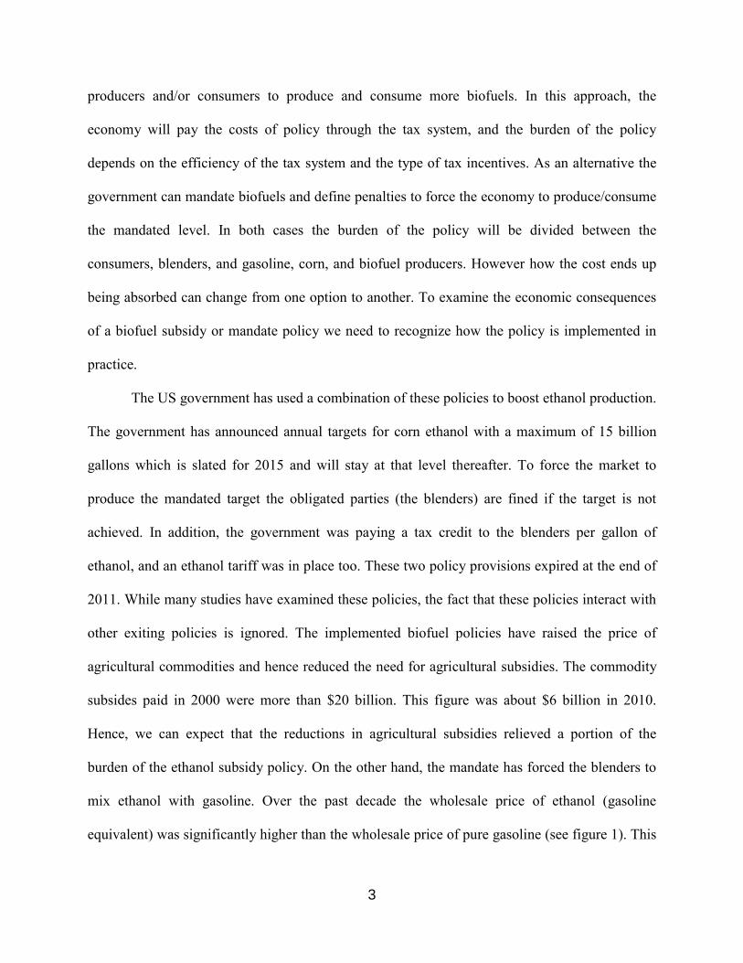
The US government has used a combination of these policies to boost ethanol production.

The government has announced annual targets for corn ethanol with a maximum of 15 billion

gallons which is slated for 2015 and will stay at that level thereafter. To force the market to

produce the mandated target the obligated parties (the blenders) are fined if the target is not

achieved. In addition, the government was paying a tax credit to the blenders per gallon of

ethanol, and an ethanol tariff was in place too. These two policy provisions expired at the end of

2011. While many studies have examined these policies, the fact that these policies interact with

other exiting policies is ignored. The implemented biofuel policies have raised the price of

agricultural commodities and hence reduced the need for agricultural subsidies. The commodity

subsides paid in 2000 were more than $20 billion. This figure was about $6 billion in 2010.

Hence, we can expect that the reductions in agricultural subsidies relieved a portion of the

burden of the ethanol subsidy policy. On the other hand, the mandate has forced the blenders to

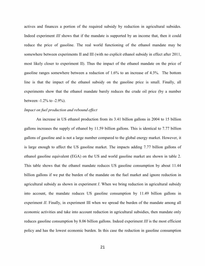
mix ethanol with gasoline. Over the past decade the wholesale price of ethanol (gasoline

equivalent) was significantly higher than the wholesale price of pure gasoline (see figure 1). This

4

means that the price of the blended fuel was higher in cost than pure gasoline, and the economy

has paid the higher price due to the mandate. One can consider the difference between the prices

of gasoline and ethanol (gasoline equivalent) as an implicit tax on the blended fuel. Of course

consumers and producers shared the burden of this implicit tax. To correctly assess the economic

impacts of the ethanol policy the explicit and implicit component of this policy and the interplay

between the mandate and other exiting tax policies should be recognized and taken into account.

This paper develops analytical and numerical general equilibrium models to examine the

importance of the implicit and explicit portions of the USA ethanol policy and their interactions

with other pre-exiting distortionary policies (such as agricultural or income taxes) for the

economic analyses of this policy. In this paper we first develop a stylized analytical general

equilibrium framework which represents interactions between economic activities and

government policies in a simple economy. The stylized analytical model is developed based on

the work done by Goulder et al. (1999) and Taheripour et al. (2008). The first paper examined

the cost effectiveness of alternative air pollution reduction policies in a second-best setting, and

the second paper analyzed welfare impacts of alternative polices for agricultural pollution control

again in a second best setting. The analytical work decomposes the welfare impacts of a

representative mandate policy into several components and shows how they affect welfare and

interact with the implemented policy. The analytical work also indicates how the economy

substitutes ethanol with gasoline and examines under what conditions the mandate could induce

a rebound effect. Then we use a computable general equilibrium model to quantify the economic

impacts of the US ethanol policy. For the numerical analyses we rely on the GTAP-BIO-ADV

model developed by Taheripour, Tyner, and Wang (2011).

2. Literature Review

5

The economic and environmental consequences of the US ethanol mandate have been

examined from different angles using a wide range of economic modeling approaches. Many

papers have used partial equilibrium models and highlighted the economic implications of this

policy for the US economy. Early studies in this area examined the role of ethanol as an additive

to gasoline and argued that using ethanol as an alternative for MTBE (another oxygenate) could

increase economic welfare and reduce emissions (for example see Gallagher et al. 2003). Several

papers examined the importance of government fixed ethanol subsidy for agricultural and energy

markets and its economic consequences. In this context Gardner (2007) examined the choice

between crop and ethanol subsidies and claimed that a deficiency payment program (a direct

subsidy to corn producers) that costs the same to tax payer as ethanol subsidy will induce an

annual deadweight losses of $37 million in long run. His corresponding estimate for the

deadweight loss of ethanol subsidy was about $665 million. He missed the fact that an increase

in ethanol subsidy could reduce the need for agricultural subsidies. Tyner and Quear (2006) and

Tyner and Taheripour (2007) showed that replacing the fixed per gallon ethanol subsidy with a

variable-rate subsidy could reduce the social costs of the government intervention and still

protect the ethanol industry from the adverse consequences of down ward shifts in crude price.

Taheripour and Tyner (2007) and de Gorter and Just (2007) studied the efficiency and

distributive effects of a biofuel subsidy. Rajagopal et al. (2007) argued that the ethanol tax credit

reduces the price of gasoline by 3% and could improve the welfare of the US economy by $11

billion. On the other hand, de Gorter and Just (2009) showed that in the presence of farm

subsidies the ethanol tax credit will reduce the welfare of the US economy by $1.3 billion.

In another line of research several papers examined the implications of ethanol subsidy

for fuel demand. These papers usually employed partial equilibrium models and to argue that the

6

ethanol subsidy could reduce the price E10 and raise the demand for this product. These papers

claim that the increased demand for E10 due to the ethanol subsidy may mitigate environmental

and security benefits of ethanol production because the subsidy generates a rebound effect which

eventually leads to higher demand for gasoline and more imports of crude oil (for example: see

Vedenov and Wetzstein, (2007) and Khanna et al., (2008)). Several papers also examined the

effect of ethanol mandate on gasoline demand. For example, de Gorter and Just (2008) examine

the effects of a tax credit in the presence of a blend mandate. They showed that a tax credit with

a mandate results in a subsidy to fuel consumers and higher fuel consumption. Hochman et al.

(2010) also claimed that introducing biofuels into the energy market generates a rebound effect

at a global scale.

Almost of the analyses mentioned above are based on partial equilibrium models, which

manly highlighted consequences of the US ethanol policy for agricultural and/or fuel markets.

These analyses usually ignore the rest of the economy and disregard the fact that resources are

limited and that the biofuel mandates interact with other policies and pre-existing distortionary

taxes.

By the second half of the 2007, the importance of indirect land use emissions induced by

biofuel production were introduced in to the literature. The early papers in this field suggested

that biofuel production could have extraordinary land use implications (Tokgoz et al., 2007;

Kammen et al., 2007; Searchinger et al., 2008; Fargione et al., 2008). For example, Searchinger

et al. (2008) provided the first peer-reviewed estimate for the ILUC (about 0.73 hectares of new

cropland area per 1000 gallon of ethanol capacity). Those authors used a partial equilibrium

modeling framework (FAPRI) to assess the ILUC due to US ethanol program. However, the

more recent studies find the early estimates have overstated the land use implications of US

7

ethanol production (Hertel et al., 2010; Al-Riffai et al., 2010; EPA, 2010; Taheripour et al.,

2010; Tyner et al., 2010; and Laborde, 2011). For example, Hertel et al. (2010) using a general

equilibrium model showed that full accounting for market mediated price responses to ethanol

production, as well as the geography of world trade, contributed to significant reductions in

estimated ILUC impacts. Those authors estimated that the ILUC for the US ethanol program is

about 0.29 hectares per 1000 gallons of ethanol.

Almost all research studies which examined the induced land use changes also ignored

the that the US ethanol policy has reduced the need for agricultural subsidies and their

experiments poorly represent the way that the policy is implements in real world. In this paper

we show that including reduction in agricultural production subsidies could significantly alter the

induced land use changes due to ethanol production.

3. Why Simple Partial Equilibrium Models Could Be Misleading

In this section we employ a simple partial equilibrium model which has been frequently

used to assess the welfare impacts of biofuel policies. In this analysis it is assumed that gasoline

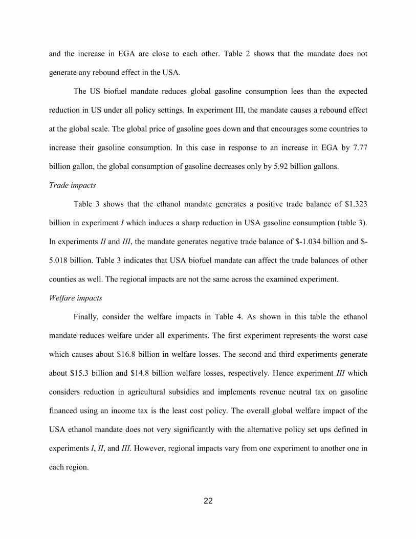
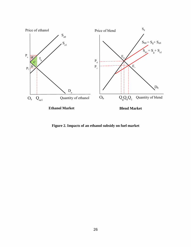
and ethanol are perfect substitutes and they have identical energy contents. Consider the left

panel of Figure 2 which represents the market for ethanol. In this market the supply of and

demand for ethanol with no government intervention are shown with Se0 and De. The demand

curve for ethanol represents the derived demand of the blender which blends ethanol with

gasoline at an arbitrary rate and supplies the blend to the market for the blended fuel. This figure

assumes that with no government support, ethanol production is zero. This means that the

marginal cost of ethanol production is higher than the blender’s willingness to pay for ethanol at

any production level of this fuel. Now assume that the government subsidizes ethanol production

with a fixed rate of te per gallon of ethanol. Ignore the fact that the government needs to finance

8

the policy. In this partial equilibrium framework the supply of ethanol will shift to Se1. With this

subsidy the equilibrium price and quantity of ethanol will be pe1 and QSe1 . At this equilibrium

the ethanol producer receives pe per gallon of ethanol and the blender pays pe1 per gallon. With

this set up the change in benefits received by the ethanol producer, the change in benefits

received by the blender, and the amounts of subsidy paid by the government are equal to the

areas of a, b, and a+b+c, respectively. The deadweight losses observed due to the ethanol

subsidy would be equal to c1. Now for a moment assume that the policy has no other welfare

impacts. With this assumption in mind now consider the right panel of Figure 2 which depicts

the market for the blended fuel. Given that the market for pure ethanol (say E85) is negligible we

assumed that the consumers only consume the blended fuel and that the curve Db represents their

demand curve for this product. When ethanol is not subsidized the supply curve of Sb = Sg+ Se0

represents the market supply. With this supply curve the market equilibrium for the blend would

be at E0 with no ethanol blended with gasoline. When the government pays ethanol subsidy then

the curve Sb = Sg+ Se1 represents the supply curve of the blend and the market equilibrium for the

blended fuel moves to E1. At this equilibrium supplies of gasoline, ethanol, and the blended fuel

would be equal to ObQg, OeQSe1=QgQ1, and ObQ1, respectively. In this situation one can

conclude that the ethanol subsidy creates a rebound effect because it increases the consumption

of the blended fuel by QoQ1.

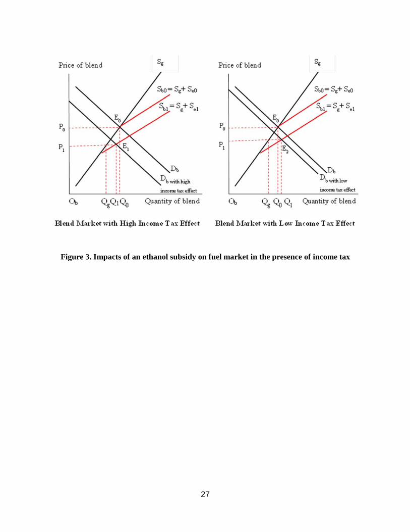
We now take into account the fact that the government needs to finance the ethanol

subsidy. There are several ways to finance the policy. Reduction in existing subsidies, an

additional fuel tax on gasoline production, an income tax, and or changing in tax rates imposed

1 The deadweight losses mention here belongs to changes in ethanol market. Ethanol subsidy could affect consumers and producers surpluses in other markets as well. A partial equilibrium model can trace the changes in consumers and producers surpluses in few other markets such as markets for corn and E10, but they fail to capture the welfare impacts through the entire economy.

9

on other goods and services are some options to finance the ethanol subsidy. Using either of

these options or a combination of them will affect the above partial equilibrium analyses. To

examine how the financing issue could alter the above rebound effect conclusion, consider a

simple income tax. The income tax shrinks the households’ disposable incomes which eventually

reduces demands for goods and services including the demand for fuel. Consider now a case

where the income elasticity of demand for fuel is high and the income tax hits the demand for

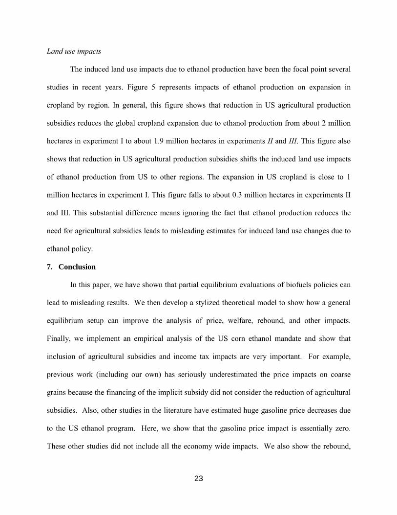
this commodity significantly. The left panel of Figure 3 represents this situation. This figure

indicates that if the induced income tax effect of the ethanol subsidy is high, then the demand

curve for ethanol shifts back significantly and no rebound effect is observed in the new

equilibrium of E1 where Q1<Q0. On the other hand, if the income elasticity of the demand for

fuel is low, then the demand shifts back slightly and results in a minor rebound effect (see the

right panel of figure 3). This simple example shows that including the possibility of an income

tax for supporting the ethanol subsidy could alter the results of our partial equilibrium analyses.

In general, studies which argued for rebound effect used partial equilibrium models which ignore

the fact that the ethanol subsidy needs to be financed through the tax system.

Consider now a case where the government does not pay any subsidy but forces a fuel

blend including a certain share of ethanol per gallon of the blend, say α. Given that the price of

ethanol is more expensive than the price of gasoline we can assume that: pe=(1+β)pg. Here pe

and pg represent the prices of ethanol and gasoline, respectively, and β>0. Following an average

pricing rule the supply price of the blend will be: pb=(1+μ)pg where μ=β(1-α)>0. Hence, in this

case the blending mandate increases the supply price of the fuel with an equivalent ad valorem

rate of μ=β(1-α)>0. The left panel of Figure 4 represents the supply curve of the blended fuel for

this case with Sb. In this panel the market equilibrium is at E1 with the equilibrium price of pb

10

(higher than the initial price of p0) and the equilibrium quantity of Qb (less than the initial

quantity of Q0). With a blending mandate in place the ethanol producer receives pe and the

gasoline price received by gasoline producer is pg. As shown in the right panel of figure 4 the

difference between these two prices represents the social costs of the mandate per gallon of

produced ethanol. In this case the partial equilibrium analysis does not produce a rebound effect

because the price paid by the consumer of the blended fuel increases due to the mandate.

However, it shows that the price received by the gasoline producer drops from p0 to pg and the

quantity of gasoline supply falls from Q0 to Qg. The reduction in gasoline price received by the

gasoline producer with reduction in gasoline consumption in a country with mandate can open

the room for other countries to expand their gasoline consumption and that could lead to a

rebound effect at the global scale. The global numerical general equilibrium analysis provided in

this paper indicates that the US ethanol mandate causes a week rebound effect at the global scale.

The above partial equilibrium analysis showed that imposing a mandate could not cause a

rebound effect in the country which imposes the mandate. This could be a misleading

conclusion. For example, in the US case the ethanol mandate could lead to increases in crop

prices, raise farmers’ incomes, increase land prices, generate higher income from trade of

commodities, reduction in agricultural subsidies, and cause many other impacts. The compound

effect of these changes could alter our conclusion from the above partial equilibrium analysis.

4. An Analytical General Equilibrium Framework

The analytical model developed in this section follows the work done by Goulder et al.

(1999). These authors employed a stylized analytical general equilibrium framework and

examined the cost effectiveness of alternative air emissions reduction policies in the presence of

pre-existing distortionary labor tax. Taheripour et al. (2008) extended their work and examined

11

the economic efficiency of agricultural pollution reduction policies in the presence of labor and

agricultural support policies. We revise this model by introducing ethanol into the modeling

structure.

Consider an open economy with three commodities - gasoline (X), ethanol (E), and food

(Y) with constant returns to scale production technologies. Gasoline consumption generates two

externality costs. It increases emissions and reduces national security. The per gallon social costs

of gasoline consumption are ω. The economy consists of three producers each producing only

one commodity; a representative consumer who consumes good and services and owns

endowments including labor ( L ), land ( R ), and capital ( K ); and a government which

determines income tax rates on labor (tL), land (tR), and capital (tK), regulates externality costs of

gasoline using a fixed tax rate (tX) per gallon of produced gasoline, supports food production

using a production subsidy (SE), regulates imports of gasoline to match the world price of

gasoline with its domestic market price using a tariff rate of tm on imported gasoline, and pays

transfer payments (G). The representative consumer derives utility from consumption of gasoline

(CX), Ethanol (CE), Food (CY), and leisure (l) and disutility from gasoline externality costs (N )

through the following utility function:

( , , , ) ( )X E Yu u C C C l Nφ= − . (1)

Here l L L= − , where L represents labor supply. The consumer receives disposable income from

work ( (1 )Lt L− : wage is the numeraire and hence equals one) and non-labor income (Q)

including capital income ( (1 )K Kt r K− : rK represents price of capital), land income ( (1 )R Rt r R− :

rR represents price of land), and government transfer payments (G: no tax on transfer payments).

The consumer allocates this income to purchase gasoline (CX), Ethanol (CE), and (CY) with

market prices of pX, pE, and pY, respectively. Hence the consumer budget constraint is:

12

(1 )X X E E Y Y Lp C p C p C t L Q+ + = − + . (2)

The economy is competitive, exports (y) some part of food production, and imports (x)

some part of its gasoline consumption. The economy imports gasoline (the dirty good) at the

world price (pXW) and exports food at domestic market price (pY). The trade is in balance as

shown in the following:

( )XW Y Yp x p y p= . (3)

Here pXW=pX-tm, where tm stands for any difference between the domestic and world prices of

gasoline, which implies a tariff/subsidy per unit of imported gasoline.

In this economy producers use Constant Returns to Scale (CRS) technologies. This

implies zero profits in production process of gasoline, ethanol, and food in a competitive market

zero profit condition. Under these assumptions the marginal and average costs are equal to each

other in the absence of regulation. These assumptions in combination with the existing

regulations introduced above imply:

( , )X X R K Xp MC r r t= + , (4)

( , )E E R K Ep MC r r S= − , (5)

( , )Y Y R K Yp MC r r S= − . (6)

Finally, with the assumptions and the regulations defined above, the government budget

constraint can be defined in as follow.

( )X X m L R R K K E E Y Yt O x t t L t r R t r K s O s O G+ + + + = + + . (7)

Here OX, OE, and OY represent outputs of gasoline, ethanol, and food. In this equation the first

two elements of the left hand side show revenues from production and imports of gasoline. Other

13

components of the left hand side measure revenues from income taxes. The right hand side of the

government constraint measures government’s payments to support ethanol and food production

and transfer payments.

In order to reduce emissions caused by gasoline consumption the government has several

options to follow in this simple economy. Some important options are: an increase in gasoline

tax, an increase in ethanol subsidy, a mandate on gasoline consumption or production, a mandate

on ethanol consumption or production, introducing a tax on emissions, introducing an emissions

reduction subsidy, and/or a combination of these policies. These policies could induce different

welfare impacts and affect the economy in different ways. Given that the US has in the past used

an ethanol tax credit, we examine the welfare impacts of an increase in ethanol subsidy to reduce

total externality costs of gasoline consumption (N =ωCY).

To achieve this goal consider a marginal increase in ethanol subsidy. To finance this

policy the government can increase income tax rates, reduce food subsidies, change gasoline

tariff rate, reduce transfer payments, or a combinations of these methods. To assess a general

case assume that all of these options are all on the table.

To determine the welfare impacts of a marginal increase in ethanol subsidy in a general

case, we differentiate the utility function with respect to SE, enforce the household budget

constraint, impose the trade balance, take into account the government budget constraint, apply

the market clearing condition, and use Slutsky equation and Shepard’s lemma and several other

microeconomic theories2. The welfare impacts are classified into several components and are

shown in the following equation:

2 A similar approach is used in Goulder et al. (1999) and Taheripour et al. (2008). The decomposition process used in this paper is available upon request from the authors.

14

E

du

dsλ=

Pr

YY

E

imary food effect

dOs

ds− ( )

Pr Re

m X X X E E E E

imary bound Effect

t O x s Oε θ ε θ+ + −

Pr

(1 ) (1 ) mX Yx X y Y

E E E E E

imary Trade Effect

dtdp dpdx dyx p y p x

ds ds ds ds dsε ε− + + + − + + (8)

Re Re

LTR

E

venue cycling Effect

dNM

ds

+

, ,

( ) JL J G

J X E Y J E

Tax Interaction Effect

dpLt C S

p dsτ τ

=

∂ ′− − + ∂ L LQ

N N

N on Labor Income Effect

L dQ dGt

Q dt dtτ ε

−

+ −

.

The first three components measure the primary impacts of an increase in ethanol

subsidy. The primary food effect is expected to be welfare improving. An increase in ethanol

subsidy moves resources away from food to ethanol production and reduces the need for food

subsidy. This item shows only the direct efficiency gain due to reduction in food subsidy. The

second terms measures the impact of rebound effect on welfare. In this component Xθ and Eθ

show percentage changes in consumption of gasoline and ethanol, and Xε and Eε stand for the

demand price elasticities of these commodities. This component could increase or decrease

welfare. In this component E E E Es O ε θ− is always welfare improving. However, ( )m X X Xt O x ε θ+

could be positive or negative. The percentage change in gasoline consumption, Xθ , determines

the sign of this subcomponent. If Xθ <0, then this subcomponent is positive and hence the overall

primary rebound effect is welfare improving. However, if Xθ >0, then the welfare impact of

primary rebound effect could be positive, negative, or zero.

The next component is the primary trade effect. In general, when the demand for the

exported food is inelastic, the world price of gasoline remains constant (or goes down), and the

15

tariff (tm) remains unchanged, then the trade effect will be welfare improving. Otherwise it could

be either positive, negative or zero.

The next component in equation 8 shows the revenue recycling effect. If the ethanol

subsidy is financed using a labor tax, then the revenue recycling effect would be welfare

decreasing. The next component is labeled tax interaction effect. The tax interaction effect

measures efficiency costs due to interaction between the ethanol and labor tax. This secondary

effect could be either positive or negative. Finally, the last component of the above equation

measures efficiency costs due to interaction between labor supply and non-labor incomes. The

policy will likely increase the price of land, which leads to an increase in leisure and reduces

labor supply. This will reduce welfare. For more detail about the last three components of

equation (8) see Taheripour et al. (2008).

We now analyze the consequences of the ethanol subsidy for the substitution between

gasoline and ethanol. Using the budget constraint defined in equation (2) in combination with

some standard derivations it is straightforward to show that:

1 11X X Y Y Y E E E

E EX E YE E X IE E X

dC C C p p

dC C C p p

ε α εε ε ε ε

+ += − − + −

. (9)

In the derivation process of this equation, it is assumed the government does not increase

income tax rates to support the ethanol subsidy. This equation indicates that the displacement

ratio between gasoline and ethanol (dCX/dCE) is a function of own and cross price elasticities,

relative prices, and relative consumption of commodities. This ratio measures rebound effect

according to the following chart:

- If dCX/dCE ≥ 0, then an increase in ethanol consumption due to an increase ethanol

consumption does not reduce consumption of gasoline. In this case total consumption of

16

fuel (CX+CE) goes up by (dCE+dCX: where dCX ≥ 0). We refer to this as strong rebound

effect.

- If 0 > dCX/dCE > -1, then an increase in ethanol consumption due to an increase in

ethanol subsidy decreases consumption of gasoline with an amount less than the increase

in ethanol production. In this case total consumption of fuel (CX+CE) goes up by

(dCE+dCX: where dCX <0). We refer to this as weak rebound effect.

- If dCX/dCE ≤ -1, then an increase in ethanol consumption due to an increase in ethanol

subsidy decreases consumption of gasoline with an amount equal or larger than the

increase in ethanol production. In this case total consumption of fuel (CX+CE) goes down

or stays the same. We refer to this case as no rebound effect.

Since ethanol is a substitute for gasoline, then > 0, and hence the first term in equation (8) is

always negative. Consider the sign of the next two components of this equation. If food and fuel

(ethanol) are compliments, then < 0. Therefore, with an inelastic food demand the second

term is positive. Finally, if the income elasticity of demand for ethanol is positive, and its own

price elasticity is less than one then the third term is positive too. With these assumptions the

displacement ratio can be either positive or negative. Hence in general an ethanol subsidy may or

may not generate a rebound effect. In general we can conclude that:

From the above analysis it clear that if ethanol and gasoline are compliments then the

first component of equation (8) will become positive. The combination of this assumption and

other assumptions on the income and price elasticities noted above implies a strong rebound

effect. This means that if ethanol is an additive for gasoline, then it is likely to observe a strong

rebound effect due to the ethanol subsidy.

17

5. N umerical Model

To evaluate the economic impacts of the US ethanol policy we modify the GTAP-BIO-

ADV model developed in Taheripour, Tyner, and Wang (2011)3. This model is designed and

used to assess the land use impacts of alternative biofuel pathways. The GTAP-BIO-ADV is a

CGE mode which takes into account the interactions between a wide range of economic

activities (including biofuels) and handles production, consumption, and trade of goods and

services at a global scale, while it allocates scarce resources such as land, labor and capital

among economic activities. This model covers production and consumption of the first and

second generation of biofuels and links them with other industries and services.

This model includes the traditional fuels markets as well. The oil, gas, and coal industries

supply materials to the processed petroleum, electricity, and other industries at the global scale.

In general, the model considers liquid biofuels (ethanol, biodiesel, and bio-gasoline), as direct

substitutes for gasoline. However, it assumes low degrees of substitutions among all energy

commodities at the firm and household levels as well.

The model takes into account the competition for land among the land use industries such

as forestry, livestock, and crop industries. Production of biofuel (except for corn stover)

increases competition for land among the land use industries. In this model cropland pasture is a

part of cropland and is an input in the production processes of the livestock industry.

The model handles the production, consumption, and trade of a wide range of

commodities at a global scale. It aggregates the world economy into 43 groups of commodities

3 The model is an advanced version of GTAP-BIO model which developed by Taheripour et al. (2010), Hertel, Tyner, and Birur (2010), and Taheripour, Hertel, and Tyner (2011) and Tyner et al. (2011).

18

(including biofuels, DDGS, and oilseed meals) and 19 regions and represents the world economy

in 2004.

The GTAP-BIO model and its successors substitute ethanol and gasoline volumetrically.

Given that the energy content of ethanol is about 67% of gasoline, the volumetric approach could

generate misleading results. To fix this problem we made proper changes in the model to

compare ethanol and gasoline based on their energy contents. We use the modified GTAP-

BIO_AEZ model to examine the economic impacts of the USA ethanol mandate.

The RFS2 is the core component of the US ethanol policy. This mandate forces the

economy to consume 15 billion gallons of corn ethanol in 2015. At the same time the mandate

has been supported by an ethanol tax credit and a trade tariff until the end of 2011. We can

consider reduction in agricultural subsidy as a portion of ethanol policy as well. To introduce all

components of the ethanol policy into the GTAP simulation process we have several options to

follow. Consider the following three options.

Option 1

To implement the mandate and enforce the market to produce and consume 15 billion

gallons of ethanol we need to introduce a market incentive into the GTAP-BIO-AEZ Model. The

market incentive could be a revenue neutral tax credit for ethanol production financed by a

gasoline tax. This method imposes the main burden of the policy on parties involved in fuel

market (ethanol producer, refineries, and fuel consumers). This method does not simulate the

actual ethanol policy, but measures the economic impacts if we ignore other components of the

policy. This method constitutes our first simulation. We refer to this simulation as experiment I.

Option 2

19

This option brings reduction in agricultural production subsidy into account. We know

that in reality ethanol production has decreased the need for agricultural production subsidies.

The GTAP model uses ad valorem subsidies and thus cannot adjust them as commodity prices

increase However, many tax rates are flexible in real world. For example, the US production

subsidies go down if crop prices go up. We fixed this problem in option 2 by reducing US

agricultural production output subsidies to zero, while other agricultural subsidies remain in

effect according to their 2004 rates presented in the base data. In this option a portion of required

ethanol subsidy comes from reduction in agricultural subsidy, and as a result, a lower gasoline

tax is required to achieve the mandated level of 15 billion gallons of ethanol. We refer to this

simulation as experiment II.

Option 3

Options 1 and 2 mainly impose the burden of the mandate policy on fuel market. In

option 3 we assume that the government cuts agricultural production subsidies, and then finances

the rest of required ethanol subsidies to produce 15 billion gallons of ethanol using an income tax

increase. This method spreads the burden of the mandate to all economic activities. We refer to

this option as experiment III.

In conclusion the above experiments can be defined as:

Experiment I: An increase in USA ethanol production from its 3.41 billion gallons in 2004 to 15

billion gallons mandated for 2015 using an incentive production subsidy per gallon of ethanol

financed using a gasoline production tax.

20

Experiment II: An increase in USA ethanol production from its 3.41 billion gallons in 2004 to 15

billion gallons mandated for 2015 using a production subsidy per gallon of ethanol financed

using a gasoline production tax and by reduction of US agricultural subsidies to zero.

Experiment III: An increase in USA ethanol production from its 3.41 billion gallons in 2004 to

15 billion gallons mandated for 2015 using a production subsidy per gallon of ethanol financed

using a an income tax and by reduction of US agricultural subsidies to zero.

6. N umerical Results

The numerical analyses provide in this section are all based on the results obtained from

the experiments introduced in the previous sections. The numerical analyses cover impacts of the

ethanol mandate on commodity prices, crude oil and gasoline prices, fuel production, trade

balance, and welfare.

Price impacts

The ethanol mandate increases market prices of crop commodities. Among the alternative

options, experiment I generates the lowest impact on crop prices. This is because this experiment

assumes that agricultural activities will continue to receive production subsidies in the presence

of the ethanol mandate. The crop price impacts obtained from experiments II and III are very

similar and significantly higher than the price impacts of experiment I. For example, experiments

I, II, and III predict that the ethanol mandate increases the price of coarse grains by about 7.2%,

16.9%, and 16.8% respectively.

On the other hand experiment I predicts the highest price impact for gasoline and crude

oil, because this experiment ignores the fact that a portion of required subsidy for ethanol is

financed due to reduction in agricultural subsidies. On the other hand, experiment III predicts the

lowest price impact for gasoline, because it spread the burden of the policy on all economic

21

actives and finances a portion of the required subsidy by reduction in agricultural subsides.

Indeed experiment III shows that if the mandate is supported by an income that, then it could

reduce the price of gasoline. The real world functioning of the ethanol mandate may be

somewhere between experiments II and III (with no explicit ethanol subsidy in effect after 2011,

most likely closer to experiment II). Thus the impact of the ethanol mandate on the price of

gasoline ranges somewhere between a reduction of 1.6% to an increase of 4.3%. The bottom

line is that the impact of the ethanol subsidy on the gasoline price is small. Finally, all

experiments show that the ethanol mandate barely reduces the crude oil price (by a number

between -1.2% to -2.9%).

Impact on fuel production and rebound effect

An increase in US ethanol production from its 3.41 billion gallons in 2004 to 15 billion

gallons increases the supply of ethanol by 11.59 billion gallons. This is identical to 7.77 billion

gallons of gasoline and is not a large number compared to the global energy market. However, it

is large enough to affect the US gasoline market. The impacts adding 7.77 billion gallons of

ethanol gasoline equivalent (EGA) on the US and world gasoline market are shown in table 2.

This table shows that the ethanol mandate reduces US gasoline consumption by about 11.44

billion gallons if we put the burden of the mandate on the fuel market and ignore reduction in

agricultural subsidy as shown in experiment I. When we bring reduction in agricultural subsidy

into account, the mandate reduces US gasoline consumption by 11.49 billion gallons in

experiment II. Finally, in experiment III when we spread the burden of the mandate among all

economic activities and take into account reduction in agricultural subsidies, then mandate only

reduces gasoline consumption by 8.06 billion gallons. Indeed experiment III is the most efficient

policy and has the lowest economic burden. In this case the reduction in gasoline consumption

22

and the increase in EGA are close to each other. Table 2 shows that the mandate does not

generate any rebound effect in the USA.

The US biofuel mandate reduces global gasoline consumption lees than the expected

reduction in US under all policy settings. In experiment III, the mandate causes a rebound effect

at the global scale. The global price of gasoline goes down and that encourages some countries to

increase their gasoline consumption. In this case in response to an increase in EGA by 7.77

billion gallon, the global consumption of gasoline decreases only by 5.92 billion gallons.

Trade impacts

Table 3 shows that the ethanol mandate generates a positive trade balance of $1.323

billion in experiment I which induces a sharp reduction in USA gasoline consumption (table 3).

In experiments II and III, the mandate generates negative trade balance of $-1.034 billion and $-

5.018 billion. Table 3 indicates that USA biofuel mandate can affect the trade balances of other

counties as well. The regional impacts are not the same across the examined experiment.

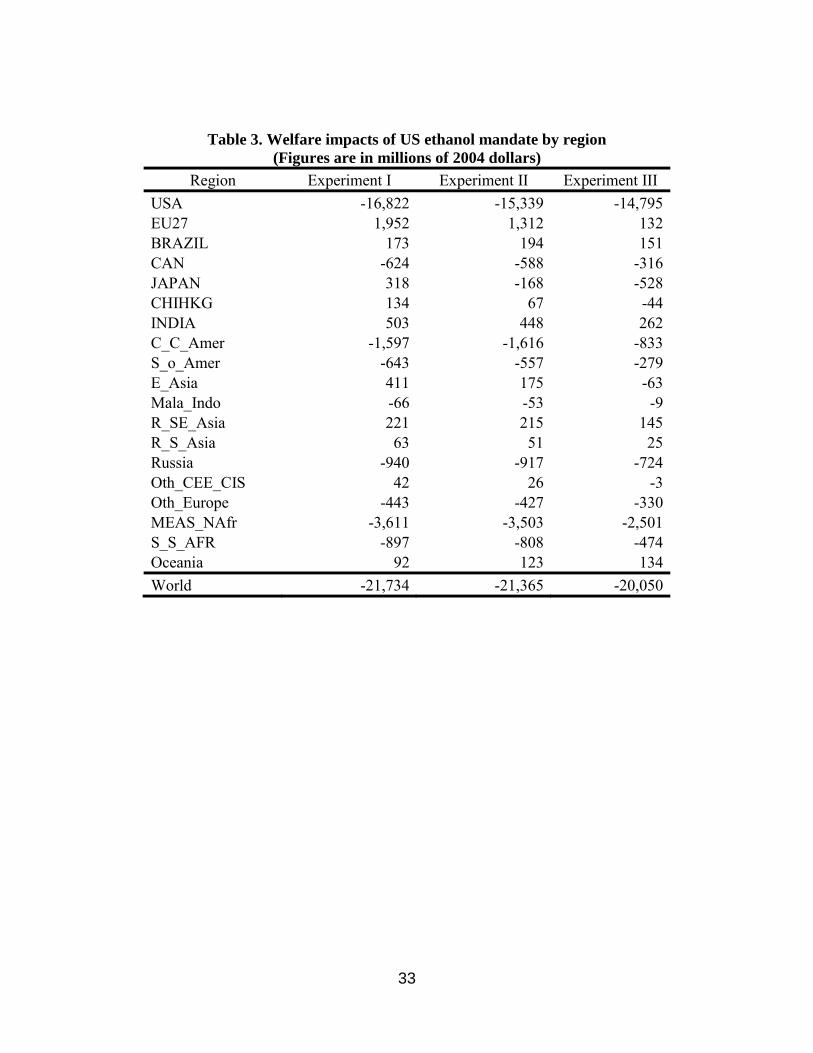
Welfare impacts

Finally, consider the welfare impacts in Table 4. As shown in this table the ethanol

mandate reduces welfare under all experiments. The first experiment represents the worst case

which causes about $16.8 billion in welfare losses. The second and third experiments generate

about $15.3 billion and $14.8 billion welfare losses, respectively. Hence experiment III which

considers reduction in agricultural subsidies and implements revenue neutral tax on gasoline

financed using an income tax is the least cost policy. The overall global welfare impact of the

USA ethanol mandate does not very significantly with the alternative policy set ups defined in

experiments I, II, and III. However, regional impacts vary from one experiment to another one in

each region.

23

Land use impacts

The induced land use impacts due to ethanol production have been the focal point several

studies in recent years. Figure 5 represents impacts of ethanol production on expansion in

cropland by region. In general, this figure shows that reduction in US agricultural production

subsidies reduces the global cropland expansion due to ethanol production from about 2 million

hectares in experiment I to about 1.9 million hectares in experiments II and III. This figure also

shows that reduction in US agricultural production subsidies shifts the induced land use impacts

of ethanol production from US to other regions. The expansion in US cropland is close to 1

million hectares in experiment I. This figure falls to about 0.3 million hectares in experiments II

and III. This substantial difference means ignoring the fact that ethanol production reduces the

need for agricultural subsidies leads to misleading estimates for induced land use changes due to

ethanol policy.

7. Conclusion

In this paper, we have shown that partial equilibrium evaluations of biofuels policies can

lead to misleading results. We then develop a stylized theoretical model to show how a general

equilibrium setup can improve the analysis of price, welfare, rebound, and other impacts.

Finally, we implement an empirical analysis of the US corn ethanol mandate and show that

inclusion of agricultural subsidies and income tax impacts are very important. For example,

previous work (including our own) has seriously underestimated the price impacts on coarse

grains because the financing of the implicit subsidy did not consider the reduction of agricultural

subsidies. Also, other studies in the literature have estimated huge gasoline price decreases due

to the US ethanol program. Here, we show that the gasoline price impact is essentially zero.

These other studies did not include all the economy wide impacts. We also show the rebound,

24

trade, and welfare impacts of the policy cases. The welfare impacts, interestingly, do not differ

significantly across the cases.

We also show that ignoring the reduction of agricultural output subsidies due to higher

coarse grain prices induced by biofuels demand leads to very misleading geographical

distribution of land use changes. Taking into account the agricultural subsidy reduction

diminishes land use change in the US by about 70%, while reducing global land use change only

about 5%.

25

Figure 1. Ethanol and unleaded gasoline average rack prices

26

Db

E1

Sg

E0

Sb0 = Sg+ Se0

Q1 Q

0

P1

P0

Qg

Se0

Se1

De

te

Qse1

P1

a

b c

Sb1

= Sg+ S

e1

Pe

Quantity of ethanol Quantity of blend

Price of ethanol Price of blend

Ethanol Market Blend Market

Ob Oe

Figure 2. Impacts of an ethanol subsidy on fuel market

27

Figure 3. Impacts of an ethanol subsidy on fuel market in the presence of income tax

28

Db

Sg

E0

QbQ0

P0

Qg

Sb with mandate

Quantity of blend

Price of blend

Blend Market with Mandate

Ob

E1

Pb

Pg

Se0

Pe

Oe Q

se1

Pg

Implicit costs of mandated blend.

Quantity of ethanol

Ethanol Market with Mandate

Price of ethanol

De

Figure 4. Impacts of an ethanol mandate for fuel market with no explicit economic incentive

29

Figure 5. Expansion in cropland due to expansion in US ethanol production

30

Table 1. Price impacts of ethanol mandate under alternative experiments (Figures are percentage changes due to ethanol shock)

Commodity Experiment I Experiment II Experiment III

Paddy Rice 2.4 7.2 6.9 Wheat 1.9 1.6 1.4 Coarse Grains 7.2 16.9 16.8 Oilseeds 2.5 2.6 2.6 Sugar Crops 3.5 0.9 0.9 Other Crops 2.5 3.0 3.0 Crude Oil -2.9 -2.5 -1.2 Gasoline 6.2 4.3 -1.6

31

Table 2. Impacts of ethanol mandate on gasoline consumption (Figures are in billion gallon gasoline equivalent except otherwise noted)

Experiments Increase in US Ethanol Supply

Reduction in US gasoline

consumption

Reduction in global gasoline consumption

US rebound effect*

Global rebound effect*

Experiment I 7.77 -12.44 -9.36 -1.60 -1.21 Experiment II 7.77 -11.49 -8.62 -1.48 -1.11 Experiment III 7.77 -8.06 -5.92 -1.04 -0.76 *Rebound effect is defined as: Reduction in gasoline / Increase in ethanol

32

Table 3. Impacts of ethanol mandate on trade balance by region (Figures are in millions of 2004 dollars)

Region Experiment I Experiment II Experiment III

USA 1,323 -1,034 -5,018 EU27 -413 505 2,343 BRAZIL 18 67 130 CAN 10 56 141 JAPAN -101 309 1,054 CHIHKG 222 369 498 INDIA -65 -12 105 C_C_Amer 228 403 411 S_o_Amer -157 -80 42 E_Asia -12 24 78 Mala_Indo 1 30 46 R_SE_Asia -40 23 111 R_S_Asia -7 8 44 Russia -329 -301 -245 Oth_CEE_CIS -46 4 120 Oth_Europe -30 6 55 MEAS_NAfr -640 -515 -223 S_S_AFR 26 74 148 Oceania 14 62 160

33

Table 3. Welfare impacts of US ethanol mandate by region (Figures are in millions of 2004 dollars)

Region Experiment I Experiment II Experiment III

USA -16,822 -15,339 -14,795 EU27 1,952 1,312 132 BRAZIL 173 194 151 CAN -624 -588 -316 JAPAN 318 -168 -528 CHIHKG 134 67 -44 INDIA 503 448 262 C_C_Amer -1,597 -1,616 -833 S_o_Amer -643 -557 -279 E_Asia 411 175 -63 Mala_Indo -66 -53 -9 R_SE_Asia 221 215 145 R_S_Asia 63 51 25 Russia -940 -917 -724 Oth_CEE_CIS 42 26 -3 Oth_Europe -443 -427 -330 MEAS_NAfr -3,611 -3,503 -2,501 S_S_AFR -897 -808 -474 Oceania 92 123 134

World -21,734 -21,365 -20,050

34

References (incomplete)

- Al-Riffai, P., Dimaranan B., and Laborde D. 2010. Global trade and environmental impact

study of the EU biofuels mandate. International Food Policy Research Institute, Washington,

DC, USA (2010).

- de Gorter, H., and D.R. Just. 2007. “The welfare economics of an excise-tax exemption for

biofuels.” Working Paper 13, Department of Applied Economics and Management, Cornell

University, Ithaca, NY.

- de Gorter, H. and D. Just. 2008. “The law of unintended consequences: How the U.S. biofuel

tax credit with a mandate subsidizes oil consumption and has no impact on ethanol

consumption”, Department of Applied Economics and Management, Cornell University,

Ithaca, New York, USA.

- de Gorter, H., and D. Just. 2009. “The welfare economics of a biofuel tax credit and the

interaction effects with price-contingent farm subsidies.” American Journal of Agricultural

Economics 91(2): 477-488.

- Gallagher, P., H. Shapouri, J. Price, G. Schamel, and H. Brubaker. 2003. “Some long-run

effects of growing markets and renewable fuel standards on additives markets and the US

ethanol industry.” J. Pol. Modeling 25(6–7):585–608.

- Hertel, T., A. Golub, A. Jones, M. O’Hare, R. Pelvin, and D. Kammen. 2010. “Effects of US

maize ethanol on global land use and greenhouse gas emissions: Estimating market-mediated

responses”. BioScience, 60(3), 223-231.

- EPA. 2010. “Renewable fuel standard program (RFS2) regulatory impact analysis, ” United

States Environmental Protection Agency, Washington, DC, USA.

35

- Fargione, J., J. Hill, D. Tilman, S. Polasky, and P. Hawthorne. 2008. “Land clearing and the

biofuel carbon debt,” Science, 319(5867), 1235–1238.

- Gardner, B. 2007. “Fuel ethanol subsidies and farm price support, ” Journal of Agricultural &

Food Industrial Organization 5 article 4: 1-20.

- Goulder, L.H., I.W.H. Parry, R.C. Williams III, and D. Burtraw. 1999. “The cost-effectiveness

of alternative instruments for environmental protection in a second best setting,” Journal of

Public Economics 72:329–60.

- Hochman, G., D. Rajagopal, and D. Zilberman. 2010. “The effect of biofuels on crude oil

markets”, AgBioForum 13(2):112-118.

- Khanna, M, A. Ando, and F Taheripour. 2008. “Welfare effects and unintended consequences

of ethanol subsidies”, Review of Agricultural Economics, 30(3):411-421.

- Kammen, D.M., A.E. Farrell, R.J. Plevin, A.D. Jones, M.A. Delucchi, and G. F. Nemet. 2007.

“Energy and greenhouse impacts of biofuels: A framework for analysis,” Discussion paper 2.

Joint Transport Research Centre.

- Laborde, D. 2011. “Assessing the land use change consequences of European biofuels

policies,” International Food Policy Research Institute, Washington, DC, USA .

- Rajagopal, D., S. Sexton, D. Roland-Holst, D. Zilberman. 2007. “Challenge of biofuel: Filling

the tank without emptying the stomach?,” Environ Res Lett 2: 1−9.

- Searchinger, T., R. Heimlich, R. Houghton , F. Dong, A. Elobeid, J. Fabiosa, S. Tokgoz , D.

Hayes, and T. Yu. 2008. “Use of U.S. Croplands for biofuels increases greenhouse gases

through emissions from land-use change”. Science, 319(5867), 1238-1240.

36

- Taheripour, F., M. Khanna, and C. Nelson. 2008. “Welfare impacts of alternative policies for

environmental protection in agriculture in an open economy: A general equilibrium

framework”, American Journal of Agricultural Economics, 90 (3).

- Taheripour, F., M. Khanna, and C. Nelson 1999. “Welfare impacts of alternative policies for

environmental protection in agriculture in an open economy: A general equilibrium

framework,” American Journal of Agricultural Economics 90(3): 701-718.

- Taheripour, F. and W. Tyner. 2008. “Ethanol subsidies, who gets the benefits?,” in Outlaw,

Duffield,, and Ernstes (eds.), Biofuel, Food & Feed Tradeoffs, Proceeding of a conference held

by the Farm Foundation/USDA, at St. Louis, Missouri, April 12-13 2007, Farm Foundation,

Pak Brook, IL: 91-98.

- Taheripour, F., T. Hertel, W. Tyner, J. Bechman, and D. Birur. 2010. Biofuels and Their By-

Products: Global Economic and Environmental Implications. Biomass and Bioenergy, 34(3),

278-289.

- Tokgoz, S., A. Elobeid, J.F. Fabiosa, D.J. Hayes, B.A. Babcock, T. Yu, F. Dong, C.E. Hart,

and J.C. Beghin, 2007. Emerging Biofuels: Outlook of Effects on U.S. Grain, Oilseed, and

Livestock Markets. Staff Report 07-SR 101, Center for Agricultural and Rural Development,

Iowa State University.

- Tyner,W.E., and J. Quear. 2006. “Comparison of a fixed and variable corn ethanol subsidy.”

Choices 21 (3): 199–202.

- Tyner W. and F. Taheripour. 2007. “Renewable Energy Policy Alternatives for the Future,”

American Journal of Agricultural Economics 89(5): 1303-1310.

37

- Tyner, W., F. Taheripour, Q. Zhuang, D. Birur, and U. Baldos. 2010. Land Use Changes and

Consequent CO2 Emissions due to US Corn Ethanol Production: A Comprehensive Analysis.

Department of Agricultural Economics, Purdue University.

- Vedenov, D. and M. Wetzstein. 2008. “Toward an optimal U.S. ethanol fuel subsidy,” Energy

Econ 30 (5): 2073−2090.