Network of Excellence onEmbedded Systems Design

Welcome to the Course onReal-Time Kernels for Microcontrollers:

Theory and Practice

Scuola Superiore Sant’Anna, PisaJune 23-25, 2008

2

Course ProgramDay 1: Monday, June 23

Morning: RT scheduling & resource management (G. Buttazzo)RT kernels for embedded systems (P. Gai)

Afternoon: The FLEX development board (M. Marinoni)Erika kernel and the OSEK standard (P. Gai)

Day 2: Tuesday, June 24

Morning: Developing RT appl. with Erika (P. Gai – M. Marinoni)

Afternoon: Laboratory practice (P. Gai – M. Marinoni)

Day 3: Wednesday, June 25

Morning: Embedded Systems andWireless Communication (P. Pagano – G. Franchino)

Afternoon: Laboratory practice (P. Pagano – G. Franchino)

3

Lecture Schedule09:00 Morning Lecture - Part 1

11:00 Coffee Break

11:15 Morning Lecture - Part 2

13:00 Lunch Break

14:30 Afternoon Lecture - Part 1

16:15 Coffee Break

16:30 Afternoon Lecture - Part 2

18:00 End of Lectures

Real-Time Scheduling and Resource Management

Scuola Superiore Sant’Anna

Giorgio ButtazzoE-mail: buttazzo@sssup.it

6

GoalProvide some background of RT theory forimplementing control applications:

Background and basic concepts

Modeling real-time activities

Real-Time Task Scheduling

Timing analysis

Handling shared resources

7

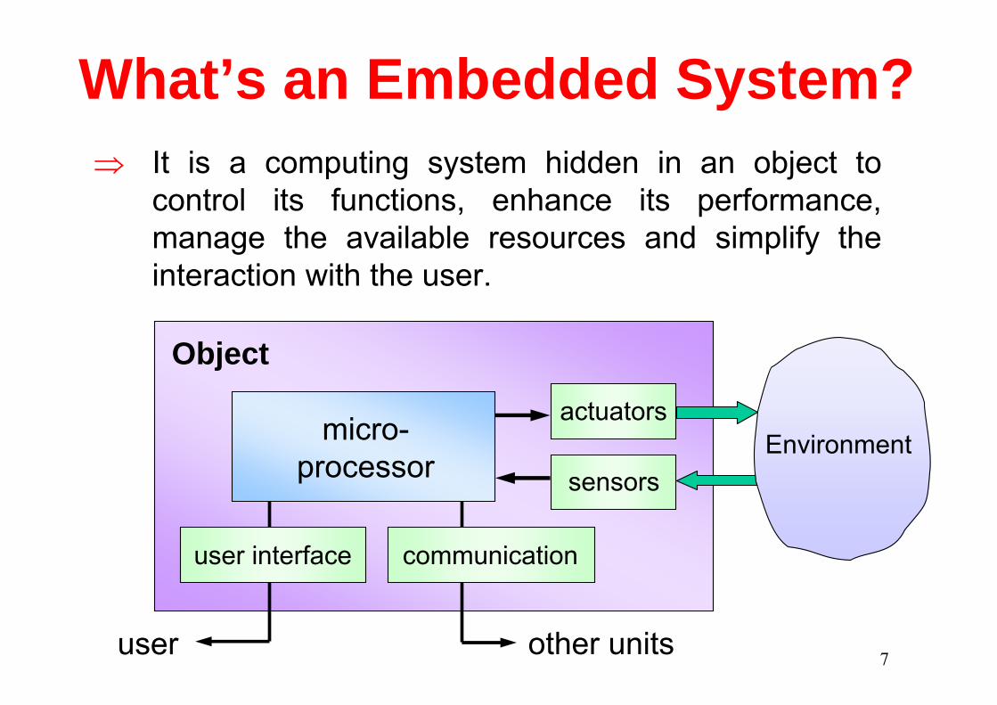
⇒ It is a computing system hidden in an object to control its functions, enhance its performance, manage the available resources and simplify the interaction with the user.

Environmentactuators

sensors

user other units

Object

communication

micro-processor

user interface

What’s an Embedded System?

What’s special in Embedded Systems?Stringent constraints on space, weight, energy, cost⇒ Scarce resources (processing power, memory)

⇒ Efficient resource usage at the OS level

Interaction with the environment⇒ High responsiveness and timing constraints

⇒ Schedulability analysis and predictable behavior (RTOS)

Robustness (tolerance to parameter variations)⇒ Overload management and system adaptation, to cope

with variable resource needs and high load variations.

9

… and many others• mobile robot systems

• small embedded devices⇒ cell phones⇒ videogames⇒ smart sensors⇒ intelligent toys

Criticality

digital tv

Timing constraints

soft firm hard

QoS management High performance Safety critical

System Requirements

digital tv

Timing constraints

soft firm hard

QoS management High performance Safety critical

efficiency predictability

12

Importance of the RTOSThe Operating System is responsible for:

managing the available resources in an efficient way (memory, devices, energy);

Enforcing timing constraints on computational activities;

Providing a standard programming interface to develop portable applications.

Providing suitable monitoring mechanisms to trace the system evolution to support debugging.

13

Software Vision

Environment

processor

actuators

sensorsA/D

D/A

Task Resource

14

Activation modes

Aperiodic tasks: (event driven)tasks are activated upon the arrival of an event(interrupt or explicit activation)

Periodic tasks: (time driven)tasks are automatically activated by the kernel at regular time intervals:

<read data><process data>

<write data><wait for next period>

buffer

buffer

<perform some action>event

15

OS support for periodic taskstask τi

wait_for_next_period();

while (condition) {

}

ready

running

idle

activeactive

idle idle

16

The IDLE state

Timer

end_cyclewake_up IDLE

dispatching

preemption

signal wait

RUNNINGREADYterminateactivate

BLOCKED

17

SLEEP state

dispatching

preemption

signal wait

end_cycle

wake_up

RUNNING

IDLE

BLOCKED

READY

Timer

terminateactivate

create sleepSLEEP

18

Periodic task modelτi (Φi , Ci , Ti , Di )

ri,k = Φi + (k−1) Ti

di,k = ri,k + Di

oftenΦi = 0 Di = Ti

ri,k ri,k+1 t

Ti

Ci

ri,1 = Φi

relativedeadline

Di

periodabsolutedeadline

di,k

19

Aperiodic task model

• Aperiodic: ri,k+1 > ri,k

• Sporadic: ri,k+1 ≥ ri,k + Ti

ri,k ri,k+1t

τiCi

ri,1

Job 1 Job 2 Job 3

20

Periodic Task Scheduling• We have n periodic tasks: {τ1 , τ2 … τn}

GoalExecute all tasks within their deadlinesVerify feasibility before runtime

τi (Ci , Ti , Di )

Assumptions• Tasks are execute in a single processor• Tasks are independent (do not block or self-suspend)• Tasks are synchronous (all start at the same time)• Relative deadlines are equal to periods (Di = Ti)

21

Timeline Scheduling(cyclic scheduling)

It has been used for 30 years in militarysystems, navigation, and monitoring systems.

Examples– Air traffic control

– Space Shuttle

– Boeing 777

22

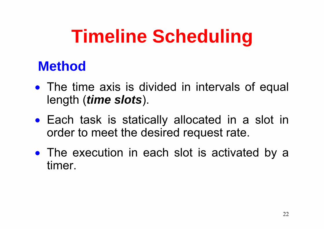
Timeline Scheduling

• The time axis is divided in intervals of equallength (time slots).

• Each task is statically allocated in a slot in order to meet the desired request rate.

• The execution in each slot is activated by a timer.

Method

23

Example

40 Hz

20 Hz

10 Hz

25 ms

50 ms

100 ms

f TA

task

B

C

∆ = GCD (minor cycle)

T = lcm (major cycle)

T

0 25 50 75 100 125 150 175 200

∆

CA + CB ≤ ∆CA + CC ≤ ∆

Guarantee:

24

Implementation

AB

AC

AB

A

timer

timer

timer

timer

minorcycle

majorcycle

25

Timeline scheduling

• Simple implementation (no real-time operating system is required).

• Low run-time overhead.

• It allows jitter control.

Advantages

26

Timeline scheduling

• It is not robust during overloads.

• It is difficult to expand the schedule.

• It is not easy to handle aperiodic activities.

Disadvantages

27

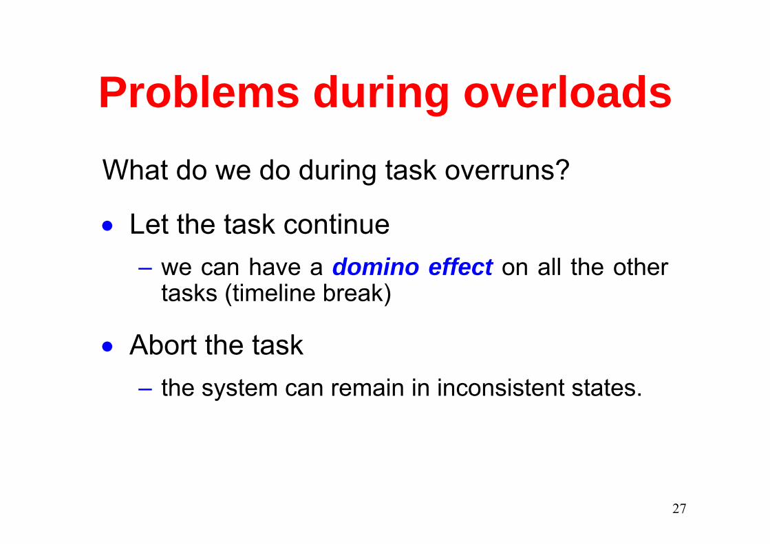
Problems during overloadsWhat do we do during task overruns?

• Let the task continue– we can have a domino effect on all the other

tasks (timeline break)

• Abort the task– the system can remain in inconsistent states.

28

ExpandibilityIf one or more tasks need to be upgraded, we may have to re-design the wholeschedule again.

Example: B is updated but CA + CB > ∆

0 25

∆

A B

29

Expandibility• We have to split task B in two subtasks

(B1, B2) and re-build the schedule:

0 25 50 75 100

B1 B1B2 B2A A A AC• • •

CA + CB1 ≤ ∆CA + CB2 + CC ≤ ∆

Guarantee:

30

ExpandibilityIf the frequency of some task is changed, the impact can be even more significant:

25 ms

50 ms

100 ms

25 ms

40 ms

100 ms

T TA

task

B

C

before after

∆ = 25 ∆ = 5T = 100 T = 200

minor cycle:major cycle:

40 sync.per cycle!

31

Example

T

0 25 50 75 100 125 150 175 200

∆

0 25 50 75 100 125 150 175 200

∆

T

32

Priority Scheduling

• Each task is assigned a priority based on itstiming constraints.

• We verify the feasibility of the schedule usinganalytical techniques.

• Tasks are executed on a priority-basedkernel.

Method

33

Priority Assignments

• Rate Monotonic (RM):pi ∝ 1/Ti (static)

• Earliest Deadline First (EDF):pi ∝ 1/di (dynamic)

ri,k ri,k+1 t

Ti

Ci

ri,1 = 0

τi (Ci , Ti , Di )

di,k = ri,k + Di

Di = Ti

34

Rate Monotonic (RM)• Each task is assigned a fixed priority

proportional to its rate.

0

500 10025 75τA

τB

0τC

40 80

100

35

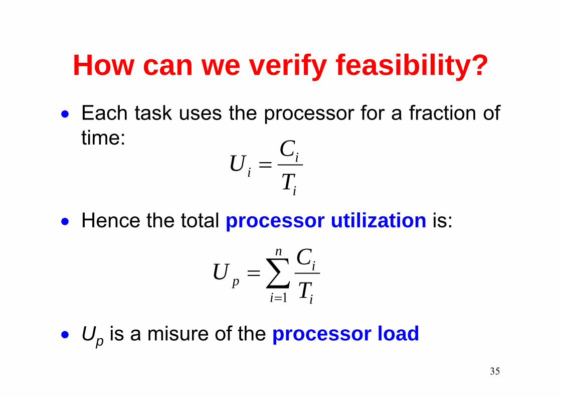
How can we verify feasibility?• Each task uses the processor for a fraction of

time:

i

ii T

CU =

• Hence the total processor utilization is:

∑=

=n

i i

ip T

CU1

• Up is a misure of the processor load

36

A necessary condition

If Up > 1 the processor is overloaded hencethe task set cannot be schedulable.

However, there are cases in which Up < 1but the task is not schedulable by RM.

37

An unfeasible RM schedule

0 9 18

6 120 183

3 6 12

9

15

15

deadline miss

τ1

τ2

944.094

63

=+=pU

38

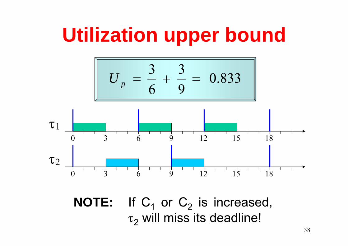
Utilization upper bound

833.093

63

=+=pU

0 9 18

6 120 183

3 6 12

9

15

15τ1

τ2

NOTE: If C1 or C2 is increased, τ2 will miss its deadline!

39

A different upper bound

184

42

=+=pU

The upper bound Uub depends on the specific task set.

0

4 120 8 16τ1

τ24 128 16

40

The least upper bound

1

Γ

Uub

Ulub

. . .

41

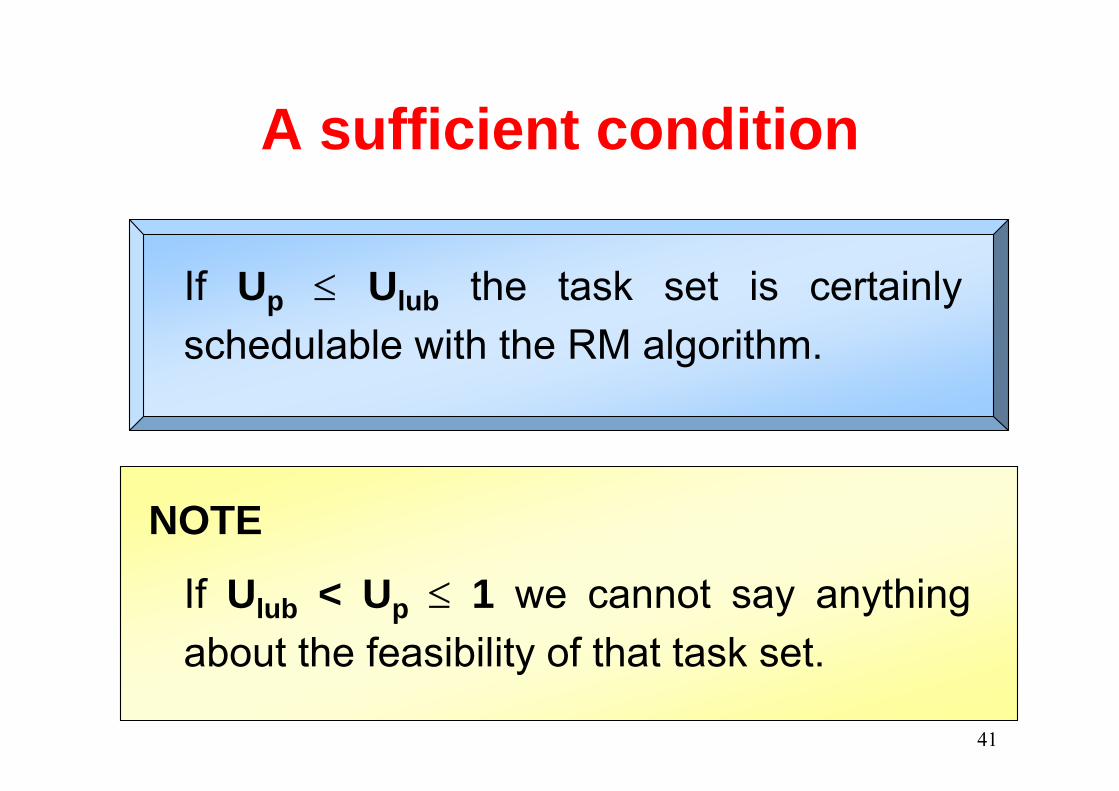
A sufficient condition

If Up ≤ Ulub the task set is certainlyschedulable with the RM algorithm.

If Ulub < Up ≤ 1 we cannot say anythingabout the feasibility of that task set.

NOTE

42

Basic results

( )121

1

−≤∑=

nn

i i

i nTCunder RM

In 1973, Liu & Layland proved that a set of nperiodic tasks can be feasibly scheduled

if

if and only ifunder EDF 11

≤∑=

n

i i

i

TC

Assumptions:Independent tasks

Di = TiΦi = 0

43

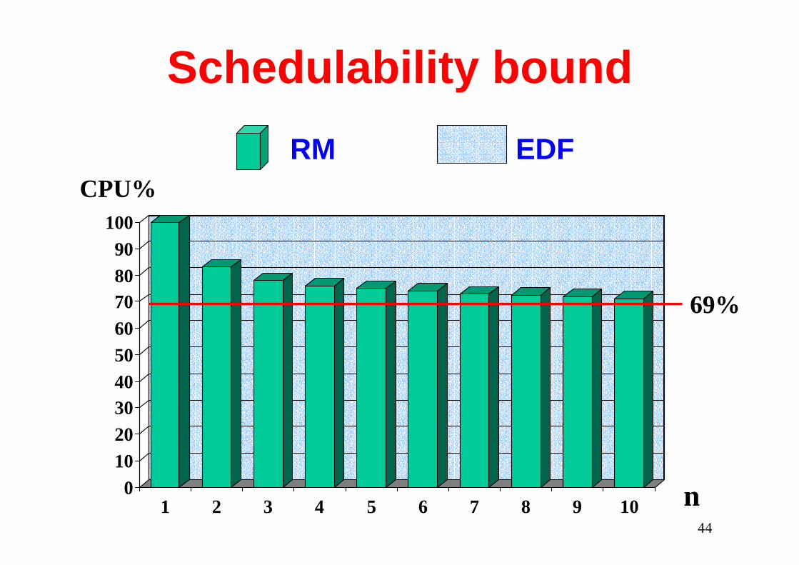
RM bound for large n

( )12 /1lub −= nRM nU

for n →∞ Ulub → ln 2

44

Schedulability bound

0102030405060708090

100

1 2 3 4 5 6 7 8 9 10

69%

n

CPU%RM EDF

45

A special case

184

42

=+=pU

If tasks have harmonic periods Ulub = 1.

0

4 120 8 16τ1

τ24 128 16

46

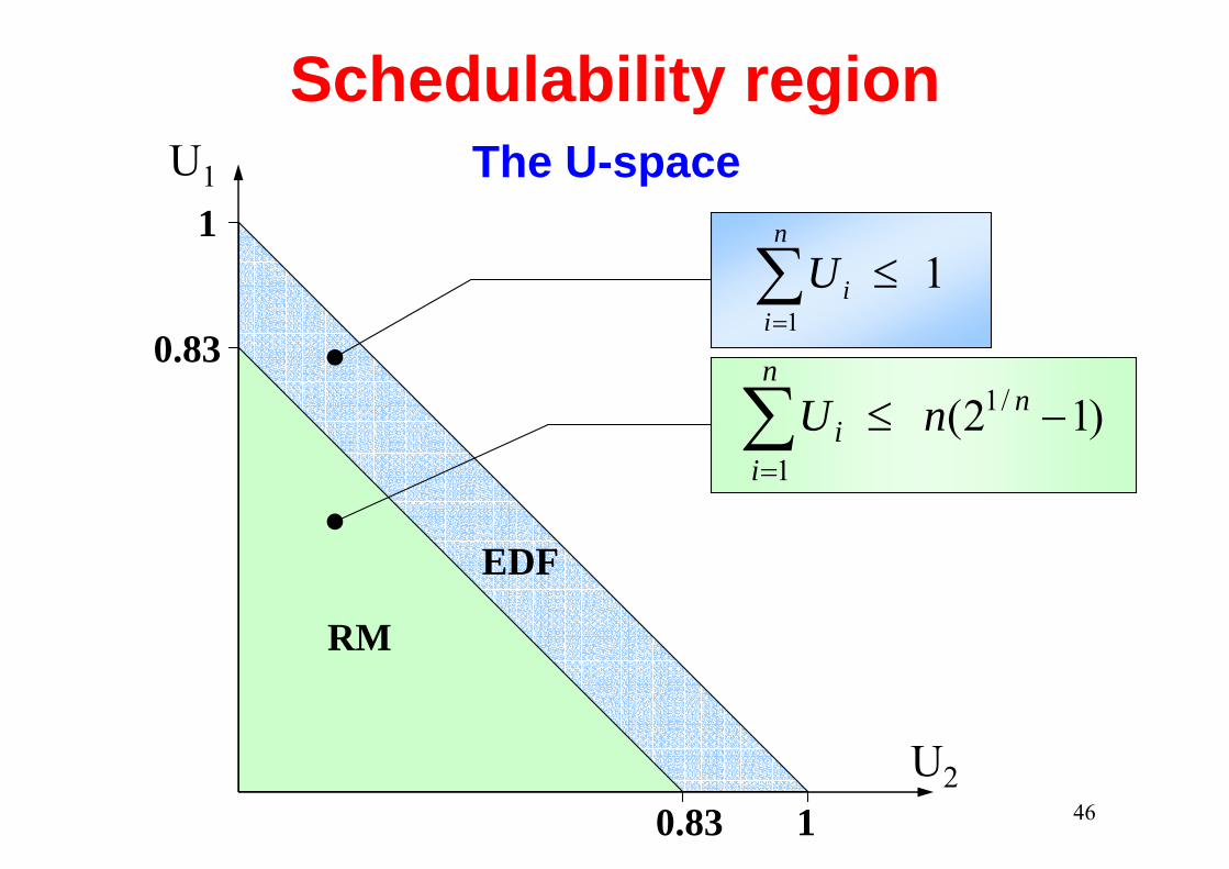
Schedulability region

1U1

U210.83

0.83

)12( /1

1

−≤∑=

nn

ii nU

11

≤∑=

n

iiU

The U-space

RM

EDF

47

Schedulability region

1U1

U210.83

0.83

The U-space

RM

EDF

τ1

τ2

Ci Ti

3

4

6

9

94.094

63

=+=pU

4/9

1/2

48

Schedule

0 9 18

6 120 183

3 6 12

9

15

15τ1

τ2

EDF

RM

0 9 18

6 120 183

3 6 12

9

15

15

deadline miss

τ1

τ2

49

RM OptimalityRM is optimal among all fixed priorityalgorithms:

If there exists a fixed priority assignmentwhich leads to a feasible schedule for Γ, then the RM assignment is feasible for Γ.

If Γ is not schedulable by RM, then itcannot be scheduled by any fixed priorityassignment.

50

EDF Optimality

EDF is optimal among all algorithms:

If there exists a feasible schedule for Γ, then EDF will generate a feasible schedule.

If Γ is not schedulable by EDF, then itcannot be scheduled by any algorithm.

51

Critical InstantFor any task τi, the longest response time occurs when itarrives together with all higher priority tasks.

τ1

τ2

R2

τ1

τ2

R2

52

The Hyperbolic Bound

• In 2000, Bini et al. proved that a set of nperiodic tasks is schedulable with RM if:

2)1(1

≤+∏=

n

iiU

53

Schedulability region

1U1

U210.83

0.83

)12( /1

1

−≤∑=

nn

ii nU

11

≤∑=

n

iiU

The U-space

RM

EDF

54

Schedulability region

1U1

U210.83

0.83

)12( /1

1

−≤∑=

nn

ii nU

11

≤∑=

n

iiU

The U-space

2)1(1

≤+∏=

n

iiU

RM

EDF

55

Extension to tasks with D < T

ri,k di,k

Ci

tτi

Di

Ti

ri,k+1

• Deadline Monotonic: pi ∝ 1/Di (static)

• Earliest Deadline First: pi ∝ 1/di (dynamic)

Scheduling algorithms

56

Deadline Monotonic

τ2

τ1

0 4 8 12 16 20 24 28

Problem with the Utilization Bound

116.163

32

1>=+== ∑

=

n

i i

ip D

CU

but the task set is schedulable.

57

How to guarantee feasibility?

ri,k di,k

Ci

tτi

Di

Ti

ri,k+1

• Fixed priority: Response Time Analysis (RTA)

• EDF: Processor Demand Criterion (PDC)

58

Response Time Analysis[Audsley ‘90]

• For each task τi compute the interferencedue to higher priority tasks:

• compute its response time asRi = Ci + Ii

• verify if Ri ≤ Di

∑<

=ik DD

ki CI

59

Computing the interference

0 Ri

τi

τk

Interference of τk on τiin the interval [0, Ri]: k

k

iik C

TRI =

Interference of highpriority tasks on τi: k

k

ii

ki C

TRI ∑

−

=

=1

1

60

Computing the response time

kk

ii

kii C

TRCR ∑

−

=

+=1

1

Iterative solution:

kk

si

i

ki

si C

TRCR

)1(1

1

−−

=∑+=

ii CR =0

iterate until)1( −> s

isi RR

61

Processor Demand Criterion[Baruah, Howell, Rosier 1990]

In any interval of time, the computationdemanded by the task set must be no greaterthan the available time.

)(),(,0, 122121 ttttgtt −≤>∀

For checking the existence of feasibile scheduleand for EDF

62

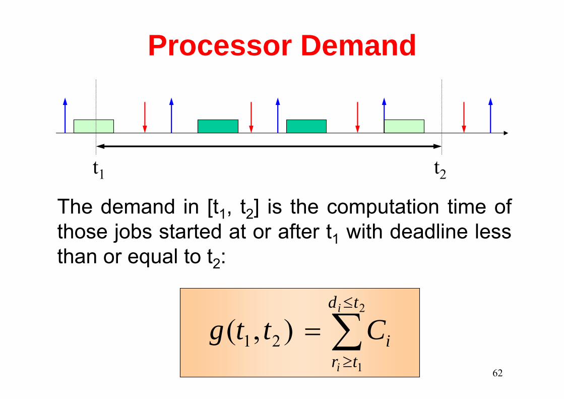
Processor Demand

t1 t2

∑≤

≥

=2

1

),( 21

td

tri

i

i

Cttg

The demand in [t1, t2] is the computation time of those jobs started at or after t1 with deadline lessthan or equal to t2:

63

Processor DemandFor synchronous task sets we can only analyze intervals [0,L]

LDi Ti + Di 2Ti + Di 3Ti + Di

0 L

τi

g(0, L) ∑=

+−=

n

ii

i

ii CT

TDL1

g(0, L)

64

Processor Demand Test

How can we bound the number of intervals in which the test has to be performed?

Question

LCT

TDLLn

ii

i

ii ≤+−

>∀ ∑=1

0

65

Example

τ2

τ1

0 2 6 124 8 10 14 16

0

2

4

6

8

g(0, L)

L

L

66

Bounding complexity• Since g(0,L) is a step function, we can check

feasibility only at deadline points.

• If tasks are synchronous and Up < 1, we can check feasiblity up to the hyperperiod H:

H = lcm(T1, … , Tn)

67

Bounding complexity• Moreover we note that: g(0, L) ≤ G(0, L)

∑=

⎟⎟⎠

⎞⎜⎜⎝

⎛ −+=

n

ii

i

ii CT

DTLLG1

),0(

i

in

iii

n

i i

i

TCDT

TCL ∑∑

==

−+=11

)(

∑=

−+=n

iiii UDTLU

1)(

68

Limiting L

g(0, L)

L

G(0, L)∑=

−+=n

iiii UDTLULG

1)(),0( L

L*

for L > L*

g(0,L) ≤ G(0,L) < L

U

UDTL

n

iiii

−

−=∑=

1

)(1*

69

Processor Demand Test

D = {dk | dk ≤ min (H, L* )}

H = lcm(T1, … , Tn)

U

UDTL

n

iiii

−

−=∑=

1

)(1*

LCT

TDLLn

ii

i

ii ≤+−

>∀ ∑=1

0U < 1 AND

A set of n periodic tasks with D ≤ T is schedulable byEDF if and only if

70

Summarizing: RM vs. EDF

RM

EDF

Di = Ti Di ≤ Ti

ΣUi ≤ 1

LL: ΣUi ≤ n(21/n –1)

HB: Π(Ui+1) ≤ 2

LLgL ≤>∀ ),0(,0

O(n)

∀i Ri ≤ Di

pseudo-polynomial

kk

ii

kii C

TRCR ∑

−

=

+=1

1

pseudo-polynomialpolynomial:

Suff.: polynomial O(n)

RTAExact pseudo-polynomial

Response Time Analysis

Processor Demand Analysis

Inter-task communicationmechanisms

• Shared memory

• Message passing ports

• Asynchonous buffers

Handling sharedresources

Problems caused bymutual exclusion

73

Critical sections τ2τ1

globlalmemory buffer

write readx = 3;y = 5;

a = x+1;b = y+2;c = x+y;

int x;int y;

wait(s)

signal(s)

wait(s)

signal(s)

74

Blocking on a semaphore

CS

τ1 τ2

CS

p1 > p2

τ1

τ2

∆

It seems that the maximum blockingtime for τ1 is equal to the length of the critical section of τ2, but …

75

priority ∆

Priority Inversion

Occurs when a high priority task is blocked bya lower-priority task a for an unbounded

interval of time.

76

Resource Access Protocols

Under fixed priorities• Non Preemptive Protocol (NPP)• Highest Locker Priority (HLP)• Priority Inheritance Protocol (PIP)• Priority Ceiling Protocol (PCP)

Under EDF• Stack Resource Policy (SRP)

77

Non Preemptive Protocol• Preemption is forbidden in critical sections.

• Implementation: when a task enters a CS, itspriority is increased at the maximum value.

PROBLEMS: high priority tasks that do not use CS may also block

ADVANTAGES: simplicity

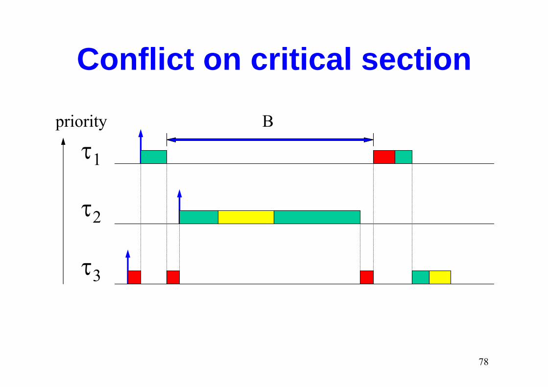
78

Conflict on critical section

τ1

priority B

τ2

τ3

79

Schedule with NPP

priority

τ1

τ2

τ3

PCS = max{P1, … Pn}

80

Problem with NPP

priority

τ1

τ2

τ3

τ1 cannot preemt, although it could

uselessblocking

81

Highest Locker Priority

A task in a CS gets the highest priorityamong the tasks that use it.

FEATURES:

• Simple implementation.

• A task is blocked when attempting to preempt, not when entering the CS.

82

Schedule with HLPpriority

τ1

τ2

τ3

τ2 is blocked, but τ1 can preempt within a CS

PCS = max {Pk | τk uses CS}

83

Problem with HLP

CS

test

τ1

CS

τ2

τ1

τ2

p1p2

τ1 blocks just in case ...

84

Priority Inheritance Protocol[Sha, Rajkumar, Lehoczky, 90]

• A task in a CS increases its priority only if itblocks other tasks.

• A task in a CS inherits the highest priorityamong those tasks it blocks.

PCS = max {Pk | τk blocked on CS}

85

Schedule with PIPpriority

τ1

τ2

τ3

p1

p3

direct blocking

push-through blocking

86

Types of blocking• Direct blocking

A task blocks on a locked semaphore

• Push-through blockingA task blocks because a lower prioritytask inherited a higher priority.

BLOCKING:a delay caused by a lower priority task

87

Identifying blocking resources• A task τi can be blocked by those

semaphores used by lower priority tasks and• directly shared with τi (direct blocking) or

• shared with tasks having priority higher than τi(push-through blocking).

Theorem: τi can be blocked at most once by each of such semaphores

Theorem: τi can be blocked at most once by each lower priority task

88

Bounding blocking times• If n is the number of tasks with priority less

than τi

• and m is the number of semaphores on which τi can be blocked, then

Theorem: τi can be blocked at most forthe duration of min(n,m) criticalsections

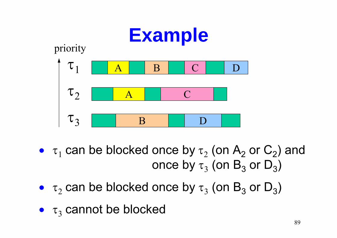
89

Examplepriority

B Cτ1

τ2

τ3

A

C

DB

A

D

• τ1 can be blocked once by τ2 (on A2 or C2) andonce by τ3 (on B3 or D3)

• τ2 can be blocked once by τ3 (on B3 or D3)

• τ3 cannot be blocked

90

Schedule with PIPpriority

τ1

τ2

τ3

τ4

P2

P1

91

Remarks on PIP

ADVANTAGES• It is transparent to the programmer.

• It bounds priority inversion.

PROBLEMS• It does not avoid deadlocks and

chained blocking.

92

Chained blocking with PIP

Theorem: τi can be blocked at most once by each lower priority task

priority B1

τ1

τ2

τ3

B2 B3

τ4

93

Priority Ceiling Protocol

• Can be viewed as PIP + access test.

• A task can enter a CS only if it is free and thereis no risk of chained blocking.

To prevent chained blocking, a task may stop at the entrance of a free CS (ceiling blocking).

94

Resource Ceilings

C(sk) = max {Pj : τj uses sk}

• Each semaphore sk is assigned a ceiling:

Pi > max {C(sk) : sk locked by tasks ≠ τi}

• A task τi can enter a CS only if

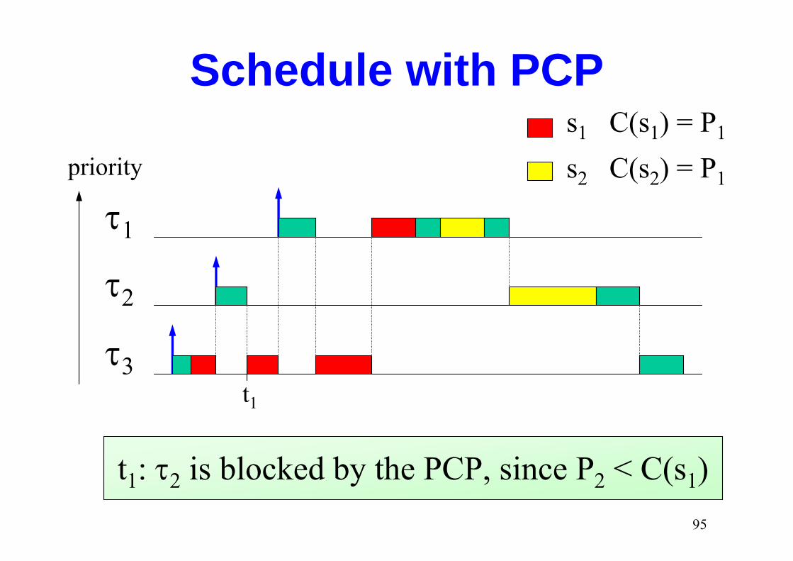
95

Schedule with PCPs1 C(s1) = P1

s2 C(s2) = P1priority

τ1

τ2

τ3t1

t1: τ2 is blocked by the PCP, since P2 < C(s1)

96

PCP propertiesTheorem 1

Under PCP, each task can block at most once.

Theorem 2

PCP prevents chained blocking.

Theorem 3

PCP prevents deadlocks.

97

Remarks on PCP

ADVANTAGES• Blocking is reduced to only one CS

• It prevents deadlocks

PROBLEMS• It is not transparent to the programmer:

semaphores need ceilings

98

Typical Deadlockτ1 τ2

τ1

τ2

blocked

blocked

P1 > P2

A

B

B

A

99

Deadlock avoidance with PCPτ1 τ2

τ1

τ2

P1 > P2

A

B

B

A

CA = P1

CB = P1

ceiling blocking

100

Guarantee with resourceconstraints

• We select a scheduling algorithm and a resource access protocol.

• We compute the maximum blocking times(Bi) for each task.

• We perform the guarantee test including the blocking terms.

101

Guarantee with RM (D = T)

preemptionby HP tasks

τi

blocking byLP tasks

( )1211

1

−≤+

+∀ ∑−

=

/i

i

iii

k k

k iT

BCTCi

By LL test:

102

Guarantee with RM (D ≤ T)

preemptionby HP tasks

τi

blocking byLP tasks

kk

ii

kiii C

TRBCR ∑

−

=

++=1

1

∀i Ri ≤ DiBy RTA test:

103

Resource Sharing under EDFThe protocols analyzed so far have been originally developed for fixed priority scheduling schemes. However:

• NPP can also be used under EDF

• PIP has been extended under EDF by Spuri (1997).

• PCP has been extended under EDF by Chen-Lin(1990)

• In 1990, Baker proposed a new protocol that works both under fixed and dynamic priorities.

104

Stack Resource Policy [Baker 1990]

• It works both with fixed and dynamicpriority

• It limits blocking to 1 critical section

• It prevents deadlock

• It supports multi-unit resources

• It allows stack sharing

• It is easy to implement

105

Stack Resource Policy [Baker 90]

• For each resource Rk:⇒ Maximum units: Nk

⇒ Available units: nk

Nk

nk

Rk

• For each task τi the system keeps:

⇒ its resource requirements:

⇒ a priority pi:

⇒ a static preemption level:

ii Tp 1∝ ii dp 1∝

ii D1∝π

RM EDF

µi(Rk)

106

Resource ceiling

System ceiling { })(max kkks nC=Π

Stack Resource Policy [Baker 90]

)(:max)( kjkjjkk RnnC µπ <=

SRP Rule

A job cannot preempt untilpi is the highest and πi > Πs

107

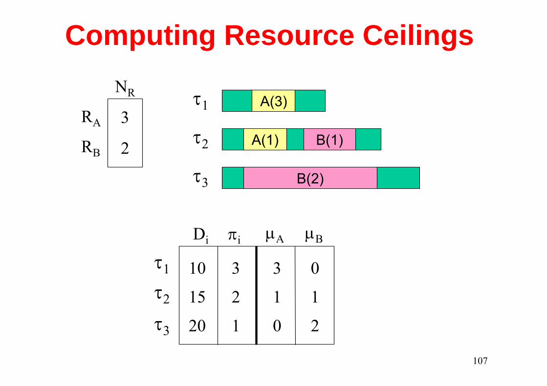
Computing Resource Ceilings NR

3

2

RA

RB

A(3)

B(1)A(1)

B(2)

τ1

τ2

τ3

τ1

τ2

τ3

Di πi

3

2

1

10

15

20

µA µB

3

1

0

0

1

2

108

Computing Resource Ceilings NR

3

2

RA

RB

CR(3)

0

-

RA

RB

CR(2) CR(1) CR(0)

3

0

3

1

3

2

τ1

τ2

τ3

Di πi

3

2

1

10

15

20

µA µB

3

1

0

0

1

2

109

Schedule with SRP

τ1

τ2

τ3

Πsπ3

π2

π1

NR CR(3) CR(2) CR(1) CR(0)0-

RA

RB

30

31

32

32

B

B B

A

A

A task blocks when attempting to preempt

A(3)

B(1)A(1)

B(2)

τ1τ2τ3

110

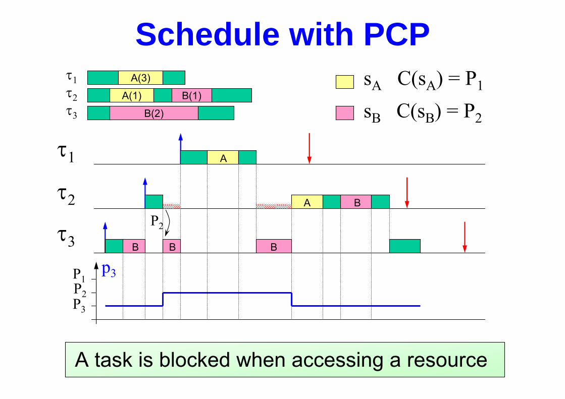
Schedule with PCP

τ1

τ2

τ3

p3

P3

P2

P1

B

B

A

A

sA C(sA) = P1

sB C(sB) = P2

B B

P2

A task is blocked when accessing a resource

A(3)

B(1)A(1)

B(2)

τ1τ2τ3

111

Lemma

SRP Properties

If πi > CR(nk) then there exist enough units of R

1. to satisfy the requirements of τi

2. to satisfy the requirements of all tasks that can make preemption on τi

112

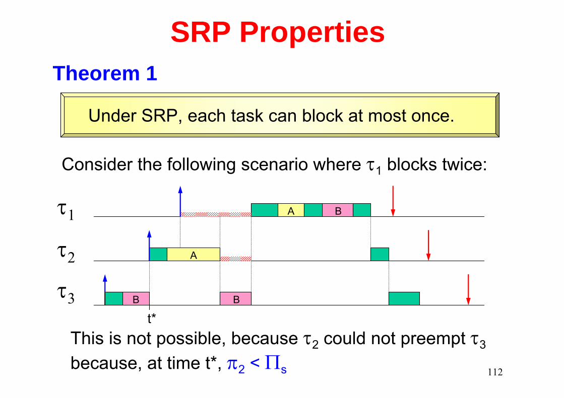
SRP PropertiesTheorem 1

Under SRP, each task can block at most once.

τ1

τ2

τ3

B

B B

A

A

Consider the following scenario where τ1 blocks twice:

This is not possible, because τ2 could not preempt τ3

because, at time t*, π2 < Πs

t*

113

SRP Properties

If πi > Πs then τi will never block once started.

Theorem 2

Since Πs = max{CR(nk)}, then there are enough resources to satisfy the requirements of τi and those of all tasks that can preempt τi .

Proof

QuestionIf a task can never block once started, can we get rid of the wait / signal primitives?

114

SRP Properties

SRP prevents deadlocks.

Theorem 3

From Theorem 2, if a task can never block once started, then no deadlock can occur.

Proof

115

Deadlock avoidance with SRPτ1 τ2

τ1

τ2

π1 > π2

A

B

B

A

116

11

1

≤+

+∀ ∑−

= i

iii

k k

k

TBC

TCi

Schedulability Analysisunder EDF

When Di = Ti

Bi can be computed as under PCP and refers to the length of longest critical section that can block τi.

117

EDF Guarantee: PD test (Di ≤ Ti )

τ1

τi

...

τk

τn

Tasks are ordered by decreasing preemption level

118

Schedulability Analysisunder EDF

When Di ≤ Ti

LCT

DTLBn

kk

k

kki ≤

−++ ∑

=1

A task set is schedulable if U < 1 and ∀L ∈ D

∀i

where D = {dk | dk ≤ min (H, L* )}

H = lcm(T1, … , Tn) U

UDTL

n

iiii

−

−=∑=

1

)(1*

119

Stack SharingEach task normally uses a private stack for

• saving context (register values)• managing functions• storing local variables

stack

stack pointerPUSH

POP

120

Stack Sharing

stack

τ1

τ2SP2

SP1

Why stack cannot be normally shared?

Suppose tasks share a resource: A

blockedbig problems

121

Stack SharingWhy stack can be shared under SRP?

stack

τ1

τ2SP2

SP1

SP2

122

Saving Stack SizeTo really save stack size, we should use a small number of preemption levels.

100 tasks

10 Kb stack per taskstack size = 1 Mb

10 preemption levels

10 tasks per groupstack size = 100 Kb

stack saving = 90 %

123

NOTE on SRPSRP for fixed priorities and single-unit resources is equivalent to Higher Locker Priority.

It is also referred to as Immediate Priority Ceiling

τ1

τ2

τ3

Πsπ3

π2

π1

B

B B

A

A

124

Non-preemtive schedulingIt is a special case of preemptive scheduling where all tasks share a single resource for their entire duration.

τ1

τ2

τ3 R

R

R

The max blocking time for task τi is given by the largest Ck among the lowest priority tasks:

Bi = max{Ck : Pk < Pi}

125

Advantages of NP scheduling• Reduces runtime overhead

Less context switches

No semaphores are needed for critical sections

• Reduces stack size, since no more than one task can be in execution.

• Preserves program locality, improving the effectiveness of

Cache memory

Pipeline mechanisms

Prefetch queues

126

• As a consequence, task execution times areSmaller

More predictable

preemptive

non-preemptive

Cmin C

Advantages of NP scheduling

127

τ1

τ20

100 205 15 25

217 14

30

28 35

35

RM

τ1

τ20

100 205 15 25

217 14

30

28 35

35

NP-RMdeadline miss

97.074

52

≅+=U

Advantages of NP schedulingIn fixed priority systems can improve schedulabiilty:

128

τ1

τ2 ∞T2

T1

C1 = ε

C2 = T1

U = ε

T1+

∞

C2 0

Disadvantages of NP scheduling• In general, NP scheduling reduces schedulability.

• The utilization bound under non preemptive scheduling drops to zero:

129

Non preemptive scheduling anomalies

τ1

τ2

τ3

τ1

τ2

τ3

deadline missdouble speed

130

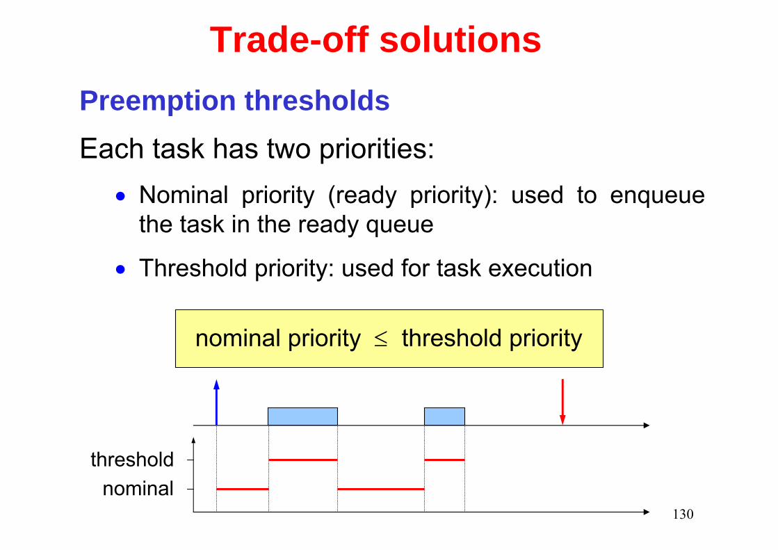
Trade-off solutionsPreemption thresholdsEach task has two priorities:

• Nominal priority (ready priority): used to enqueue the task in the ready queue

• Threshold priority: used for task execution

thresholdnominal

nominal priority ≤ threshold priority

131

Preemption thresholds

• Nominal pr. = threshold: ⇒ fully preemptive

• Threshold = Pmax ⇒ fully non preemptive

P2

P1

P3

thresholds

θ1 = P1

θ2 = P2

θ3 = P2

In general:

132

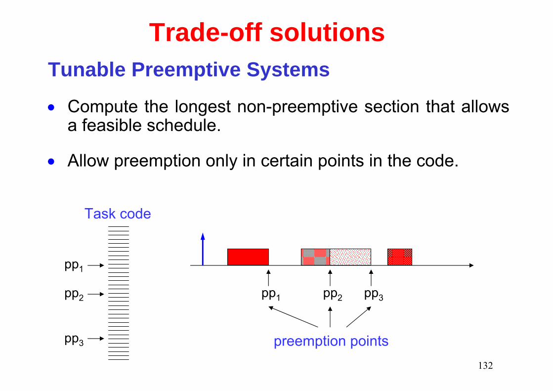
Trade-off solutionsTunable Preemptive Systems

• Compute the longest non-preemptive section that allows a feasible schedule.

• Allow preemption only in certain points in the code.

pp1

pp2

pp3

pp1 pp2 pp3

Task code

preemption points