Weighted Sum-Rate Maximization in Wireless Networks: A - Oulu
165
Foundations and Trends R in Networking Vol. 6, Nos. 1-2 (2011) 1–163 c 2012 P. C. Weeraddana, M. Codreanu, M. Latva-aho, A. Ephremides and C. Fischione DOI: 10.1561/1300000036 Weighted Sum-Rate Maximization in Wireless Networks: A Review By Pradeep Chathuranga Weeraddana, Marian Codreanu, Matti Latva-aho, Anthony Ephremides and Carlo Fischione Contents 1 Introduction 3 1.1 Motivation 4 1.2 Global Methods for WSRMax in Wireless Networks 7 1.3 Local Methods for WSRMax in Wireless Networks 8 1.4 Distributed WSRMax in Wireless Networks 10 1.5 Outline of the Volume 12 2 A Branch and Bound Algorithm 15 2.1 System Model and Problem Formulation 16 2.2 Algorithm Derivation 21 2.3 Computation of Upper and Lower Bounds 26 2.4 Extensions to Multicast Networks 37 2.5 Numerical Examples 38 2.6 Summary and Discussion 57 3 Low Complexity Algorithms 59 3.1 System Model and Problem Formulation 60 3.2 Algorithm Derivation: CGP and Homotopy Methods 66
Transcript of Weighted Sum-Rate Maximization in Wireless Networks: A - Oulu

Foundations and TrendsR© inNetworkingVol. 6, Nos. 1-2 (2011) 1–163c© 2012 P. C. Weeraddana, M. Codreanu,M. Latva-aho, A. Ephremides and C. FischioneDOI: 10.1561/1300000036
Weighted Sum-Rate Maximizationin Wireless Networks: A Review
By Pradeep Chathuranga Weeraddana,Marian Codreanu, Matti Latva-aho,
Anthony Ephremides and Carlo Fischione
Contents
1 Introduction 3
1.1 Motivation 41.2 Global Methods for WSRMax in Wireless Networks 71.3 Local Methods for WSRMax in Wireless Networks 81.4 Distributed WSRMax in Wireless Networks 101.5 Outline of the Volume 12
2 A Branch and Bound Algorithm 15
2.1 System Model and Problem Formulation 162.2 Algorithm Derivation 212.3 Computation of Upper and Lower Bounds 262.4 Extensions to Multicast Networks 372.5 Numerical Examples 382.6 Summary and Discussion 57
3 Low Complexity Algorithms 59
3.1 System Model and Problem Formulation 603.2 Algorithm Derivation: CGP and Homotopy Methods 66

3.3 Extensions to Wireless Networkswith Advanced Transceivers 80
3.4 Numerical Examples 863.5 Summary and Discussion 109
4 A Distributed Approach 111
4.1 System Model and Problem Formulation 1124.2 Problem Decomposition, Master Problem,
and Subproblems 1154.3 Distributed Algorithm 1244.4 Numerical Examples 1314.5 Summary and Discussion 139
5 Conclusions 141
A Improving Upper Bound for Branchand Bound via ComplementaryGeometric Programming 145
B The Barrier Method 147
Acknowledgments 149
Notations and Acronyms 150
References 152

Foundations and TrendsR© inNetworkingVol. 6, Nos. 1-2 (2011) 1–163c© 2012 P. C. Weeraddana, M. Codreanu,M. Latva-aho, A. Ephremides and C. FischioneDOI: 10.1561/1300000036
Weighted Sum-Rate Maximizationin Wireless Networks: A Review
Pradeep Chathuranga Weeraddana1,Marian Codreanu2, Matti Latva-aho3,
Anthony Ephremides4 and Carlo Fischione5
1 Automatic Control Lab, KTH Royal Institute of Technology, Stockholm,100-44, Sweden, [email protected]
2 Centre for Wireless Communications, University of Oulu, Oulu, 90014,Finland, [email protected]
3 Centre for Wireless Communications, University of Oulu, Oulu, 90014,Finland, [email protected]
4 University of Maryland, College Park, MD, 20742, USA,[email protected]
5 Automatic Control Lab, KTH Royal Institute of Technology, Stockholm,100-44, Sweden, [email protected]
Abstract
A wide variety of resource management problems of recent inter-est, including power/rate control, link scheduling, cross-layer control,network utility maximization, beamformer design of multiple-inputmultiple-output networks, and many others are directly or indirectlyreliant on the weighted sum-rate maximization (WSRMax) problem.In general, this problem is very difficult to solve and is NP-hard. Inthis review, we provide a cohesive discussion of the existing solution

methods associated with the WSRMax problem, including global, fastlocal, as well as decentralized methods. We also discuss in depth theapplications of general optimization techniques, such as branch andbound methods, homotopy methods, complementary geometric pro-gramming, primal decomposition methods, subgradient methods, andsequential approximation strategies, in order to develop algorithmsfor the WSRMax problem. We show, through a number of numericalexamples, the applicability of these algorithms in various applicationdomains.

1Introduction
Consider a general wireless network with L interfering links. Theachievable rate of each link is a scalar function and is denoted by rl.Then the general weighted sum-rate maximization (WSRMax) problemhas the form:
maximize∑L
l=1 βlrl(y)subject to y ∈ Y.
(1.1)
Here y = (y1, . . . ,yn) is the optimization variable of the problem, pos-itive scalar βl is the weight associated with link l, and the (possiblynonconvex) set Y is the feasible set of the problem. In general, rl is notconvex in y. Therefore, problem (1.1) is surprisingly difficult to solve,though it appears to be very simple.
In this section, we first provide a discussion that emphasizes theimportance of WSRMax problem (1.1) in wireless networks. Next wediscuss the importance of global, fast local, as well as distributed solu-tion methods for WSRMax problem. Finally, the existing key literaturethat address the problem is presented. Applications of optimizationtechniques for developing algorithms for the problem will be covered inlater sections, with more technical detail.
3

4 Introduction
1.1 Motivation
Among various resource management policies, the WSRMax foran arbitrary set of interfering links plays a central role in manynetwork control and optimization methods. For example, the prob-lem is encountered in network utility maximization (NUM) [88], theresource allocation (RA) subproblem in various cross-layer control poli-cies [43, 81], MaxWeight link scheduling in multihop wireless net-works [120], power/rate allocation in wireless networks, as well as inwireline networks [115, 124], joint optimization of transmit beamform-ing patterns, transmit powers, and link activations in multiple-inputmultiple-output (MIMO) networks [34], and finding achievable rateregions of singlecast/multicast wireless networks [87], among others.
1.1.1 Network Utility Maximization (NUM)
In the late nineties, Kelly et al. [59, 60] introduced the concept of NUMfor fairness control in wireline networks. It was shown therein thatmaximizing the sum-rate under the fairness constraint is equivalentto maximizing certain network utility functions and different networkutility functions can be mapped to different fairness criteria. For auseful discussion of many aspects of the NUM concept in the case ofwireless network, see [88] and the references therein. In this context,the WSRMax problem appears as a part of the Lagrange dual problemof the overall NUM problem; see [89] and the references therein.
1.1.2 Cross-layer Control Policies for Wireless Networks
For useful discussions of cross-layer control policies, see [40, 43, 68, 71,81, 90, 142] and the references therein. Many of these policies are essen-tially identical. It has been shown that an optimal cross-layer controlpolicy, which achieves data rates arbitrarily close to the optimal oper-ating point, can be decomposed into three subproblems that are nor-mally associated with different network layers. Specifically, flow controlresides at the transport layer, routing and in-node scheduling1 resides
1 in-node scheduling refers to selecting the appropriate commodity and it is not to be con-fused with the links scheduling mechanism which is handled by the resource allocationsubproblem [43].

1.1 Motivation 5
at the network layer, and resource allocation (or RA) is usually associ-ated with the medium access control and physical layers [43]. The firsttwo subproblems are convex optimization problems and can be solvedrelatively easily. It turns out that under reasonably mild assumptions,the RA subproblem can be cast as a general WSRMax problem overthe instantaneous achievable rate region [43]. The weights of the linksare given by the differential backlogs and the policy resembles the well-known backpressure algorithm introduced by Tassiulas and Ephremidesin [120, 121] and further extended by Neely to dynamic networks withpower control; see [81] and the references therein.
1.1.3 MaxWeight Link Scheduling for Wireless Networks
Maximum weighted link scheduling for wireless networks [41, 68, 105,120, 121, 138] is a place, in which the problem of WSRMax is directlyused. Note that, for networks with fixed link capacities, the maximumweighted link scheduling problem reduces to the classical maximumweighted matching problem and can be solved in polynomial time [68].However, no solution is known for the general case when the link ratesdepend on the power allocation of all other links.
1.1.4 Power/rate Control Policies
We see sometimes that the WSRMax problem is directly used asthe basis for the power/rate control policy in wireless, as well as inwireline networks [115, 124]. For example, in DSL networks, thereis considerable research on resource management policies, which relydirectly on the WSRMax problem for multiuser spectrum balanc-ing [3, 27, 28, 39, 74, 94, 97, 127, 128, 129, 139, 140]. Direct applicationof WSRMax as an optimization criterion can also been seen exten-sively in joint power control and subcarrier assignment algorithms forOFDMA networks [7, 50, 54, 67, 104, 106, 145].
1.1.5 Resource Management in MIMO Networks
There are also a number of resource management algorithms in mul-tiuser MIMO networks, which rely on the problem of WSRMax. Forexample, the methods proposed in [34, 35, 111, 122] rely on WSRMax

6 Introduction
for joint design of linear transmit and receive beamformers. In addition,many references have applied WSRMax directly as an optimization cri-terion for beamformer design in MIMO networks, e.g., [45, 151].
1.1.6 Finding Achievable Rate Regions in WirelessNetworks
In multiuser systems many users share the same network resources, forexample, time, frequency, codes, space, etc. Thus, there is naturally atradeoff between the achievable rates of the users. In other words, onemay require to reduce its rate if another user wants a higher rate. Insuch multiuser systems, the achievable rate regions are important sincethey characterize the tradeoff achievable by any resource managementpolicy [124]. By invoking a time sharing argument, one can alwaysassume that the rate region is convex [124]. Therefore, any boundarypoint of the rate region can be obtained by using the solution of aWSRMax problem for some weights.
Thus, WSRMax is a central component in many network designproblems as we discussed above. Unfortunately, the general WSRMaxproblem is not yet amendable to a convex formulation [76]. In fact,it is NP-hard [75]. Therefore, we must rely on global optimizationapproaches [5, 52] for computing an exact solution of the WSRMaxproblem. Such global solution methods are increasingly importantbecause they can be used to provide performance benchmarks byback-substituting them into any network design method, which relieson WSRMax. They are also very useful for evaluating the perfor-mance loss encountered by any heuristic algorithm for the WSRMaxproblem.
Although global methods find the solution of the WSRMax problem,they are typically slow. Even small problems, with a few tens ofvariables, can take a very long time to solve WSRMax. Therefore, it isnatural to seek suboptimal algorithms for WSRMax that are efficientenough, and still close to optimal; the compromise is optimality [22].Such algorithms are of central importance since they can be fastand widely applicable in large-scale network control and optimizationmethods.

1.2 Global Methods for WSRMax in Wireless Networks 7
Due to the explosion of problem size and the signal overheadrequired in centralized network control and optimization methods, it ishighly desirable to develop decentralized variants of those algorithms.Therefore, finding distributed methods for the WSRMax problem is ofcrucial importance from a theoretical, as well as from a practical per-spective for decentralized implementation of many network control andoptimization methods, such as those investigated in [81, 120].
1.2 Global Methods for WSRMax in Wireless Networks
The general WSRMax problem is NP-hard [75]. It is therefore naturalto rely on global optimization approaches [5, 52] for computing an exactsolution. One straightforward approach is based on exhaustive searchin the variable space [28]. The main disadvantage of this approachis the prohibitively expensive computational complexity, even in thecase of very small problems. A better approach is to apply branchand bound techniques [52], which essentially implement the exhaustivesearch in an intelligent manner; see [3, 39, 57, 97, 129, 135, 139]. Branchand bound methods based on difference of convex functions (DC) pro-gramming [52] have been proposed in [3, 39, 139] to solve (a subclassof) WSRMax. Although DC programming is the core of their algo-rithms, it also limits the generality of their method to the problems inwhich the objective function cannot easily be expressed as a DC [52].For example, in the case of multicast wireless networks, expressing theobjective function as a DC cannot be easily accomplished, even whenShannon’s formula is used to express the achievable link rates. Anotherbranch and bound method has been used in [129] in the context ofDSL bit loading, where the search space is discretized in advance. Asa result of discretization, this method does not allow a complete con-trol of the accuracy of the solution. An alternative optimal methodwas proposed in [97], where the WSRMax problem is cast as a gener-alized linear fractional program [96] and solved via a polyblock algo-rithm [48]. The method works well for small scale problems, but aspointed out in [5, chap. 2, pp. 40–41] and [96, sec. 6.3], it may showmuch slower convergence than branch and bound methods as the prob-lem size increases. A special form of the WSRMax problem is presented

8 Introduction
in [23, p. 78] [128], where the problem data and the constraints mustobey certain properties and, consequently, the problem can be reducedto a convex formulation. However, these required properties correspondto very unlikely events in wireless/wireline networks, and therefore themethod has a very limited applicability.
1.3 Local Methods for WSRMax in Wireless Networks
The worst case computational complexity for solving the general WSR-Max problem by applying global optimization approaches can increasemore than polynomially with the number of variables. As a result, thesemethods are prohibitively expensive, even for off line optimization ofmoderate size networks. Therefore, the problem of WSRMax deservesefficient algorithms, which even though suboptimal, perform well inpractice.
Several approximations have been proposed for the case when alllinks in the network operate in certain signal-to-interference-plus-noiseratio (SINR) regions. For example, the assumption that the achievablerate is a linear function of the SINR (i.e., low SINR region) is widelyused in the ultra-wide-band systems, e.g., [98]. Other references, whichprovide solutions for the power and rate control in low SINR regionsinclude [37, 69, 99]. The high SINR region is treated in [29, 58, 86].However, at the optimal operating point different links correspondto different SINR regions, which is usually the case with multihopnetworks. Therefore, all methods mentioned above that are based oneither the low or the high SINR assumptions can fail to solve thegeneral problem.
One promising method is to cast the WSRMax problem intoa signomial program (SP) formulation [20, sec. 9] or into a com-plementary geometric program (CGP) [6, 30], where a suboptimalsolution can be obtained efficiently; we can readily convert an SPto a CGP and vice versa [30, sec. 2.2.5]. Applications of SP andCGP, or closely related solution methods, have been demonstratedin various signal processing and digital communications problems,e.g., [30, 31, 34, 35, 78, 94, 122, 127]. There are a number of other impor-tant papers proposing suboptimal solution methods for the WSRMax

1.3 Local Methods for WSRMax in Wireless Networks 9
problem, such as [2, 27, 33, 45, 68, 70, 74, 105, 111, 116, 131, 151],among others.
Though the suboptimal methods mentioned above, includingSP/CGP based algorithms, can perform reasonably well in many cases,2
it is worth pointing out that not all of them can handle the generalWSRMax problem. The reason is the self-interference problem, whicharises when a node transmits and receives simultaneously in the samefrequency band. Since there is a huge imbalance between the trans-mitted signal power and the received signal power of nodes, the trans-mitted signal strength is typically few orders of magnitude larger thanthe received signal strength. Thus, when a node transmits and receivessimultaneously in the same channel, the useful signal at the receiver ofthe incoming link is overwhelmed by the transmitted signal of the nodeitself. As a result, the SINR values at the incoming link of a node thatsimultaneously transmits in the same channel is very small. Therefore,the self-interference problem plays a central role in WSRMax in generalwireless networks [133].
Thus, in the case of general multihop wireless networks, theWSRMax problem must also cope with the self-interference problem.Under such circumstances SP/CGP cannot be directly applicable evento obtain a better suboptimal solution, since initialization of the algo-rithms is critical. One approach to dealing with self interference con-sists of adding supplementary combinatorial constraints, which preventany node in the network from transmitting and receiving simultane-ously [13, 14, 24, 38, 46, 61, 71, 138]. This is sometimes called thenode-exclusive interference model; only subsets of mutually exclusivelinks can simultaneously be activated in order to avoid the large selfinterference encountered if a node transmits and receives in the samefrequency band. Of course, such approaches induce a combinatorialnature for the WSRMax problem in general. The combinatorial natureis circumvented in [134], where homotopy methods (or continuationmethods) [4] together with complementary geometric programming [6]are adopted to derive efficient algorithms for the general WSRMax
2 For example, when a node does not transmits and receives simultaneously in the samefrequency band.
10 Introduction
problem. Here, the term “efficient” can mean faster convergence, orconvergence to a point with better objective value.
1.4 Distributed WSRMax in Wireless Networks
The emergence of large scale communication networks, as well asaccompanying network control and optimization methods with hugesignalling overheads triggered a considerable body of recent researchon developing distributed algorithms for resource management, see [21,79, 141] and the references therein. Such distributed algorithms relyonly on local observations and are carried out with limited access toglobal information. These algorithms essentially involve coordinatingmany local subproblems to find a solution to a large global problem. Itis worth emphasizing that the convexity of the problems is crucial indetermining the behavior of the distributed algorithms [21, chap. 9]. Forexample, in the case of nonconvex problems such algorithms need notconverge, and if they do converge, they need not converge to an opti-mal point, which is the case with the WSRMax problem. Nevertheless,finding even a suboptimal yet distributed method is crucial for deploy-ing distributively many network control and optimization methods,e.g., [41, 68, 81, 83, 84, 105, 118, 120, 138], which rely on WSRMax.
Distributed implementation of the WSRMax problem has beeninvestigated in [27, 93, 94, 127, 144] in the context of digital sub-scriber loops (DSL) networks. Those systems are inherently consistingof single-input and single-output (SISO) links. Related algorithms forSISO wireless ad hoc networks and SISO orthogonal frequency divi-sion multiple access cellular systems are found in [53, 117, 147, 146].However, in the case of multi antenna cellular systems, the decisionvariables space is, of course, larger, for example, joint optimizationof transmit beamforming patterns, transmit powers, and link activa-tions is required. Therefore, designing efficient distributed methods forWSRMax is a more challenging task due to the extensive amount ofmessage passing required to resolve the coupling between variables. Inthe sequel, we limit ourselves to basic, but still very important, resultsthat develop distributed coordinated algorithms for resource manage-ment in networks with multiple antennas.
1.4 Distributed WSRMax in Wireless Networks 11
Several distributed methods for WSRMax in multiple-input andsingle-output (MISO) cellular networks have been proposed in [10, 11,72, 95, 130, 132, 136]. Specifically, in [95] a two-user MISO interferencechannel (IC)3 is considered and a distributed algorithm is derived byusing the commonly used high SINR approximation [29]. Moreover,another approximation, which relies on zero forcing (ZF) beamformingis introduced in [95] to address the problem in the case of multiuserMISO IC.
The methods proposed in [10, 11, 130] derived the necessary (butnot sufficient) optimality conditions for the WSRMax problem and usedit as the basis for their distributed solution. However, many parame-ters must be selected heuristically to construct a potential distributedsolution and there is, in general no systematic method for finding thoseparameters. In particular, the algorithms in [10, 11] are designed forsystems with very limited backhaul signaling resources and do notconsider any iterative base station (BS) coordination mechanism toresolve the out-of-cell interference coupling. Even though the methodproposed in [130] relies on stringent requirements on the message pass-ing between BSs during each iteration of the algorithm, their resultsshow that BS coordination can provide considerable gains comparedto uncoordinated methods. An inexact cooperate descent algorithm forthe case where each BS is serving only one cell edge user has beenproposed in [72]. The method proposed in [66] is designed for sum-ratemaximization and uses high SINR approximation. A cooperative beam-forming algorithm is proposed in [152] for MISO IC, where each BS cantransmit only to a single user. Their proposed method employs an iter-ative BS coordination mechanism to resolve the out-of-cell interferencecoupling. However, the convexity properties exploited for distributionof the problem are destroyed when more than one user is served byany BS. Thus, their proposed method is not directly applicable to theWSRMax problem. Recently, an interesting distributed algorithm forWSRMax is proposed by Shi et al. [110], which exploits a nontrivialequivalence between the WSRMax problem and a weighted sum mean
3 K-user MISO IC means that there are K transmitter–receiver pairs, where the transmittershave multiple antennas and the receivers have single antennas.

12 Introduction
squared error minimization problem. This algorithm relies on user ter-minal assistance, such as signal covariance estimations, computationand feedback of certain parameters form user terminals to BSs overthe air interface. In practice, performing perfect covariance estimationand perfect feedback during each iteration can be very challenging. Inthe presence of user terminal imperfections, such as estimation andfeedback errors, the algorithms performance can degrade and its con-vergence can be less predictable.
Algorithms based on game theory are found in [49, 55, 65, 107,108, 109]. Their proposed methods are restricted to interference chan-nels, for example, MISO IC, MIMO IC. The methods often require thecoordination between receiver nodes and the transmitter nodes duringalgorithm’s iterations.
Many optimization criteria other than the weighted sum-rate havebeen considered in references [12, 113, 123, 143, 148, 149, 150] to dis-tributively optimize the system resources (e.g., beamforming patterns,transmit powers, etc.) in multi antenna cellular networks. In particu-lar, the references [12, 148, 149, 150] used the characterization of thePareto boundary of the MISO interference channel [56] as the basisfor their distributed methods. Their proposed methods do not employany BS coordination mechanism to resolve the out-of-cell interferencecoupling. In [113, 123, 143] distributed algorithms have been derivedto minimize a total (weighted) transmitted power or the maximum perantenna power across the BSs subject to SINR constraints at the userterminals.
1.5 Outline of the Volume
Section 2 presents a solution method, based on the branch andbound technique, which solves globally the nonconvex WSRMaxproblem with an optimality certificate. Efficient analytic boundingtechniques are introduced and their impact on convergence is numer-ically evaluated. The considered link-interference model is generalenough to model a wide range of network topologies with variousnode capabilities, for example, single- or multipacket transmission

1.5 Outline of the Volume 13
(or reception), simultaneous transmission and reception. Diverse appli-cation domains of WSRMax are considered in the numerical results,including cross-layer network utility maximization and maximumweighted link scheduling for multihop wireless networks, as well as find-ing achievable rate regions for singlecast/multicast wireless networks.
Section 3 presents fast suboptimal algorithms for the WSRMaxproblem in multicommodity, multichannel wireless networks. First, thecase where all receivers perform singleuser detection4 is considered andalgorithms are derived by applying complementary geometric program-ming and homotopy methods. Here we apply the algorithms within ageneral cross-layer utility maximization framework to examine quan-titative impact of gains that can be achieved at the network layer interms of end-to-end rates and network congestion. In addition, we show,through examples, that the algorithms are well suited for evaluating thegains achievable at the network layer when the network nodes employself interference cancelation techniques with different degrees of accu-racy. Finally, a case where all receivers perform multiuser detectionis considered and solutions are presented by imposing additional con-straints, such as that only one node can transmit to others at a timeor that only one node can receive from others at a time.
Section 4 presents an easy to implement distributed method for theWSRMax problem in a multicell multiple antenna downlink system.The algorithm is based on primal decomposition and subgradientmethods, where the original nonconvex problem is split into a mas-ter problem and a number of subproblems (one for each base station).A sequential convex approximation strategy is used to address thenonconvex master problem. Unlike the recently proposed minimumweighted mean-squared error based algorithms, the method presentedhere does not rely on any user terminal assistance. Only base stationto base station synchronized signalling via backhaul links. All the nec-essary computation is performed at the BSs. Numerical experiments
4 That is, a receiver decodes each of its intended signals by treating all other interferingsignals as noise.
14 Introduction
are provided to examine the behavior of the algorithm under differentdegrees of BS coordination.
Finally, in Section 5, we present our conclusions. The detailed workpresented in this volume is based on the research performed by theauthors that led to several recent journal and conference publications.

2A Branch and Bound Algorithm
In this section we present a branch and bound method for solving glob-ally the general WSRMax problem for a set of interfering links. At eachstep, the algorithm computes upper and lower bounds for the optimalvalue. The algorithm terminates when the difference between the upperand the lower bounds is within a pre-specified accuracy level. Efficientanalytic bounding techniques are introduced and their impact on theconvergence is numerically evaluated. The considered link-interferencemodel is general enough to model a wide range of network topolo-gies with various node capabilities, for example, single- or multipackettransmission (or reception), simultaneous transmission and reception.In contrast to the other branch and bound based techniques [3, 39, 139],the method presented here does not rely on the convertibility of theproblem into a DC problem. Therefore, it applies to a broader classof WSRMax problems (e.g., WSRMax in multicast wireless networks).Moreover, the method discussed here is not restricted to WSRMax; itcan also be used to maximize any system performance metric that canbe expressed as a Lipschitz continuous and increasing function of SINRvalues.
15
16 A Branch and Bound Algorithm
The branch and bound method given in this section shows someanalogy to the one proposed in [129] in terms of the initial searchdomain and the basic bounding techniques. However, the two methodsare fundamentally different in terms of branching techniques, as thealgorithm proposed in [129] is designed specifically to search over adiscrete space whilst the method here is optimized for a continuoussearch space. We also provide improved bounding techniques whichsubstantially improve the convergence speed of the algorithm.
Given its generality, the algorithm can be adapted to a wide range ofnetwork control and optimization problems. Performance benchmarksfor various network topologies can be obtained by back-substitutingit into any network design method which relies on WSRMax. Severalapplications, including cross-layer network utility maximization andmaximum weighted link scheduling for multihop wireless networks, aswell as finding achievable rate regions for singlecast/multicast wirelessnetworks, are presented. As suboptimal but low-complex algorithmsare typically used in practice, the given algorithm can also be used forevaluating their performance loss.
2.1 System Model and Problem Formulation
The network considered consists of a collection of nodes which cansend, receive, and relay data across a set of links. The set of allnodes is denoted by N and we label the nodes with the integer valuesn = 1, . . . ,N . A link is represented as an ordered pair (i, j) of distinctnodes. The set of all links is denoted by L and we label the links withthe integer values l = 1, . . . ,L. We define tran(l) as the transmitter nodeof link l, and rec(l) as the receiver node of link l. The existence of a linkl ∈ L implies that a direct transmission is possible from node tran(l)to node rec(l). Note that, in the most general case, L may consist ofa combination of wireless and wireline links, for example, in the caseof hybrid networks. We define O(n) as the set of links that are out-going from node n, and I(n) as the set of links that are incoming tonode n. Furthermore, we denote the set of transmitter nodes by Tand the set of receiver nodes by R, i.e., T = {n ∈ N|O(n) �= ∅} andR = {n ∈ N|I(n) �= ∅}.
2.1 System Model and Problem Formulation 17
(a) (b) (c) (d)
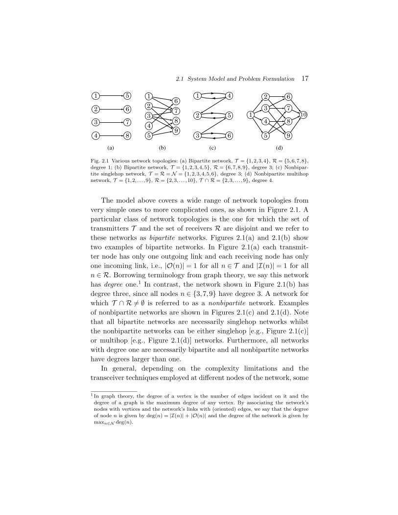
Fig. 2.1 Various network topologies: (a) Bipartite network, T = {1,2,3,4}, R = {5,6,7,8},degree 1; (b) Bipartite network, T = {1,2,3,4,5}, R = {6,7,8,9}, degree 3; (c) Nonbipar-tite singlehop network, T = R = N = {1,2,3,4,5,6}, degree 3; (d) Nonbipartite multihopnetwork, T = {1,2, . . . ,9}, R = {2,3, . . . ,10}, T ∩ R = {2,3, . . . ,9}, degree 4.
The model above covers a wide range of network topologies fromvery simple ones to more complicated ones, as shown in Figure 2.1. Aparticular class of network topologies is the one for which the set oftransmitters T and the set of receivers R are disjoint and we refer tothese networks as bipartite networks. Figures 2.1(a) and 2.1(b) showtwo examples of bipartite networks. In Figure 2.1(a) each transmit-ter node has only one outgoing link and each receiving node has onlyone incoming link, i.e., |O(n)| = 1 for all n ∈ T and |I(n)| = 1 for alln ∈ R. Borrowing terminology from graph theory, we say this networkhas degree one.1 In contrast, the network shown in Figure 2.1(b) hasdegree three, since all nodes n ∈ {3,7,9} have degree 3. A network forwhich T ∩ R �= ∅ is referred to as a nonbipartite network. Examplesof nonbipartite networks are shown in Figures 2.1(c) and 2.1(d). Notethat all bipartite networks are necessarily singlehop networks whilstthe nonbipartite networks can be either singlehop [e.g., Figure 2.1(c)]or multihop [e.g., Figure 2.1(d)] networks. Furthermore, all networkswith degree one are necessarily bipartite and all nonbipartite networkshave degrees larger than one.
In general, depending on the complexity limitations and thetransceiver techniques employed at different nodes of the network, some
1 In graph theory, the degree of a vertex is the number of edges incident on it and thedegree of a graph is the maximum degree of any vertex. By associating the network’snodes with vertices and the network’s links with (oriented) edges, we say that the degreeof node n is given by deg(n) = |I(n)| + |O(n)| and the degree of the network is given bymaxn∈N deg(n).

18 A Branch and Bound Algorithm
nodes may have restricted transmit and receive capabilities. For exam-ple, certain nodes may have only singlepacket receive and/or trans-mit capabilities2 and some nodes may not be able to transmit andreceive simultaneously. These limitations create subsets of mutuallyexclusive links and induce a combinatorial nature for the power andrate optimization in the case of networks with degree larger thanone [9, 25, 26, 62, 68, 112, 138]. An example is the maximum weightedlink scheduling for multihop wireless networks [120].
We assume that all links share a common channel and the inter-ference is controlled via power allocation. We denote the channel gainfrom the transmitter of link i to the receiver of link j by hij . For anypair of distinct links i �= j, we denote the interference coefficient fromlink i to link j by gij . In the case of nonadjacent links (i.e., links i
and j do not have a common node), gij represents the power of theinterference signal at the receiver node of link j when one unit ofpower is allocated to the transmitter node of link i, i.e., gij = |hij |2.When links i and j are adjacent (i.e., links i and j do have a com-mon node), the value of gij also depends on the transmit and receivecapabilities of the common node. Specifically, we set gij = ∞ if linksi and j are mutually exclusive and gij = |hij |2 if links i and j can besimultaneously activated. Thus, gij = gji = ∞ for any pair of mutuallyexclusive links. Figure 2.2 illustrates three examples of choosing thevalue of the interference coefficient in the case of adjacent links. Notethat in the case of nonbipartite networks, when i ∈ O(n) and j ∈ I(n),the term gij represents the power gain within the same node from itstransmitter to its receiver, and is referred to as the self-interferencecoefficient [see Figure 2.2(c)]. In the case of wireless networks, thesegains can be several orders of magnitude larger than the power gainsbetween distinct nodes. References [47, 100, 102, 119] discuss variousself interference cancelations techniques that provide different degreesof accuracy. When such schemes are employed, gij models the residualself-interference coefficient after a certain (imperfect) self interferencecancelation technique was performed.
2 We say that a node has singlepacket receive capability if it can only receive from a singleincoming link at a time. Similarly, we say that a node has singlepacket transmit capabilityif it can transmit only through a single outgoing link at a time.

2.1 System Model and Problem Formulation 19
(a) (b) (c)
Fig. 2.2 Choosing the value of interference coefficient in the case of adjacent links: (a)i, j ∈ I(n), gij = gji = ∞ if node n has singlepacket receive capability or gij = |hii|2, gji =|hjj |2 if node n has multipacket receive capability; (b) i, j ∈ O(n), gij = gji = ∞ if node nhas singlepacket transmit capability or gij = |hjj |2, gji = |hii|2 if node n has multipackettransmit capability; (c) i ∈ O(n), j ∈ I(n), gij = gji = ∞ if node n can not transmit andreceive simultaneously or gij = |hij |2 and gji = |hji|2 if node n can transmit and receivesimultaneously.
It is worth noting that the interference model described previouslycan easily be extended to accommodate different multiple access tech-niques by appropriately reinterpreting the interference coefficients. Forexample, in the case of wireless CDMA networks, the interference coef-ficient gij would model the residual interference at the output of thedespreading filter of node rec(j) [124]. Similarly, in the case of wirelessSDMA networks, where nodes are equipped with multiple antennas,gij represents the equivalent interference coefficient measured at theoutput of the antenna combiner of node rec(j) [124]. Extensions toa multichannel scenario (e.g., FDMA or FDMA-SDMA networks) arealso possible by introducing multiple links between nodes, one link foreach available spectral channel, and by setting gij = 0 if links i and j
correspond to orthogonal channels. However, many such extensions arebeyond the main scope of this volume.
We consider the case where all receiver nodes are using singleuserdetection (i.e., a receiver decodes each of its intended signals by treatingall other interfering signals as noise) and assume that the achievablerate of link l is given by
rl = log
(1 +
gllpl
σ2 +∑
j �=l gjlpj
), (2.1)
where pl is the power allocated to link l, σ2 represents the power ofthe thermal noise at the receiver, and gll represents the power gain

20 A Branch and Bound Algorithm
of link l, i.e., gll = |hll|2. The use of the Shannon formula3 for theachievable rate in (2.1) is common practice (see, e.g., [115, 124]) but itmust be noted that this is not strictly correct in the case of finite lengthpackets. However, as the packet length increases, it is asymptoticallycorrect.
Let us first consider the case of singlecast networks, where all linkscarry different information. Let βl denote an arbitrary nonnegativenumber which represents the weight associated with link l. Assumingthat the power allocation is subject to a maximum power constraint∑
l∈O(n) pl ≤ pmaxn for each transmitter node n ∈ T ,4 the problem of
weighted sum-rate maximization can be expressed as
maximize∑
l∈L βl log(
1 +gllpl
σ2 +∑
j �=l gjlpj
)subject to
∑l∈O(n) pl ≤ pmax
n , n ∈ Tpl ≥ 0, l ∈ L,
(2.2)
where the variable is (pl)l∈L.In the case of multicast networks, a transmitter can simultaneously
send common information to multiple receiver nodes. We consider thegeneral case where each transmitter node can have several multicasttransmissions. Thus, for each n ∈ T we partition O(n) into Mn disjointsubsets of links, i.e., O(n) = ∪Mn
m=1Om(n), where Mn is the number ofmulticast transmissions from node n and the set Om(n) contains alllinks associated with the mth multicast transmission of node n (seeFigure 2.3). Let pm
n and βmn be the power and the nonnegative weight
allocated to the mth multicast transmission of node n. Moreover, letp = (pm
n )n∈T , m=1,...,Mn and denote the SINR of the lth link belongs to
3 The algorithm presented in this section can be used for any other rate versus SINR depen-dence. The only restriction is that the rate must be a nondecreasing and Lipschitz contin-uous function of SINR.
4 For the sake of clarity we only consider the case of sum-power constraints for each trans-mitter node. However, supplementary sum-power constraints can be also handled by thegiven algorithm. For example, in the case of a cellular downlink employing the cooper-ation of several multiantenna base stations, sum-power constraints per subsets of nodes(one subset of nodes corresponds to a base station) should be also considered [122].

2.2 Algorithm Derivation 21
Fig. 2.3 Multicast network: Different line styles represent different multicast transmissions.T = {1,2}, M1 = 2, M2 = 1, O1(1) = {1,2}, O2(1) = {3,4}, and O1(2) = {5,6}.
the mth multicast transmission of the nth node by SINRmln (p), where
SINRmln (p)=
gllpmn
σ2+∑
j∈T ,j �=n
∑Mj
k=1 pkj maxi∈Ok(j)
gil+∑Mn
k=1,k �=m pkn max
i∈Ok(n)gil
for all n ∈ T , m = 1, . . . ,Mn. (2.3)
Clearly, for any link in the mth multicast transmission of node n, i.e.,l ∈ Om(n), interference at rec(l) is created by the other multicast trans-missions of node n itself and by multicast transmissions of other nodes.The max(·) operator in the denominator of SINR expressions is usedto impose mutually exclusive multicast transmissions, for example, ifnode 6 in Figure 2.3 has singlepacket reception capability, then O2(1)and O1(2) are mutually exclusive.
Thus, by noting that the maximum rate achievable by all links inOm(n) is given by rm
n = minl∈Om(n) rl, the weighted sum-rate maxi-mization problem can be expressed as
maximize∑
n∈T∑Mn
m=1 βmn min
l∈Om(n)log
(1 + SINRml
n (p))
subject to∑Mn
m=1 pmn ≤ pmax
n , n ∈ Tpm
n ≥ 0, n ∈ T , m = 1, . . . ,Mn,
(2.4)
where the variable is (pmn )n∈T , m=1,...,Mn .
2.2 Algorithm Derivation
For the sake of clarity, let us first address the case of single-cast networks. Extension to multicast case is presented separatelyin Section 2.4. We start by equivalently reformulating the original

22 A Branch and Bound Algorithm
problem (2.2) as minimization of a nonconvex function over an L-dimensional rectangle. Then, we present the algorithm based on abranch and bound technique [16] to minimize the nonconvex functionover the L-dimensional rectangle.
By introducing auxiliary variables γl, l ∈ L we first reformulateproblem (2.2) in the following equivalent form:
minimize∑
l∈L −βl log(1 + γl)
subject to γl ≤ gllpl
σ2 +∑
j �=l gjlpj, l ∈ L∑
l∈O(n) pl ≤ pmaxn , n ∈ T
pl ≥ 0, l ∈ L,
(2.5)
where the variables are (pl)l∈L and (γl)l∈L. The equivalence betweenproblems (2.2) and (2.5) follows from the monotone increasing propertyof the log(·) function. Clearly, any feasible γl, l ∈ L in problem (2.5)represents an achievable SINR value for link l. Let us denote the objec-tive function of problem (2.5) by f0(γ) =
∑l∈L −βl log(1 + γl) and the
feasible set for the variables γ = (γ1, . . . ,γL) (or the achievable SINRvalues) by G, i.e.,
G =
γ
∣∣∣∣∣∣∣∣γl ≤ gllpl
σ2 +∑
j �=l gjlpj, l ∈ L∑
l∈O(n) pl ≤ pmaxn , n ∈ T
pl ≥ 0, l ∈ L
. (2.6)
The optimal value of problem (2.5) can be expressed compactly ast� = inf
γ∈Gf0(γ).
For clarity, let us define a new function f : IRL+ → IR as
f(γ) ={
f0(γ) γ ∈ G0 otherwise
(2.7)
and note that for any D ⊆ IRL+ such that G ⊆ D, we have
infγ∈D
f(γ) = infγ∈G
f0(γ) = t�, (2.8)
where the first equality follows from that for any γ ∈ IRL+ we have
f0(γ) ≤ 0. It is also worth noting that the function f is nonconvex overD and f0 is a global lower bound on f , i.e., f0(γ) ≤ f(γ) for all γ ∈ D.
2.2 Algorithm Derivation 23
Let us now define the L-dimensional rectangle
Qinit ={γ∣∣0 ≤ γl ≤ σ−2gllp
maxtran(l), l ∈ L
},
which encloses the set of all achievable SINR values, i.e., G ⊆ Qinit. Byusing (2.8), it follows that
t� = infγ∈Qinit
f(γ).
Thus, we have reformulated problem (2.2) equivalently as a minimiza-tion of the nonconvex function f over the rectangle Qinit. In whatfollows we show how the branch and bound technique is used to mini-mize f over Qinit.
Let Q be a L-dimensional rectangle defined as
Q = {γ |γl,min ≤ γl ≤ γl,max, l ∈ L} ,
where γl,min and γl,max are real numbers such that γl,min ≤γl,max for all l ∈ L. For any L-dimensional rectangle Q ⊆ Qinit, let usnow define the following function:
φmin(Q) = infγ∈Q
f(γ). (2.9)
Note that
φmin(Qinit) = infγ∈Qinit
f(γ) = t�. (2.10)
The key idea of the branch and bound method is to gener-ate a sequence of asymptotically tight upper and lower bounds forφmin(Qinit). At each iteration k, the lower bound Lk and the upperbound Uk are updated by partitioning Qinit into smaller rectangles. Toensure convergence, the bounds should become tight as the number ofrectangles in the partition of Qinit grows. To do this, the branch andbound method uses two functions φub(Q) and φlb(Q), defined for anyrectangle Q ⊆ Qinit such that the following conditions are satisfied [16].
C1 : The functions φlb(Q) and φub(Q) compute a lower boundand an upper bound respectively on φmin(Q), i.e.,
∀Q ⊆ Qinit we have φlb(Q) ≤ φmin(Q) ≤ φub(Q). (2.11)
24 A Branch and Bound Algorithm
C2 : As the maximum half length of the sides of Q(i.e.,
size(Q)=12 max
l∈L{γl,max − γl,min}
)goes to zero, the difference
between the upper and lower bounds uniformly converges tozero, i.e.,
∀ε > 0 ∃δ > 0 s.t. ∀Q ⊆ Qinit,size(Q) ≤ δ
⇒ φub(Q) − φlb(Q) ≤ ε. (2.12)
For the sake of clarity, the definition and computation of φlb andφub are described in Section 2.3. In the remainder of this section wewill present the branch and bound method in more detail.
Let ε be an a priori specified tolerance. The algorithm starts bycomputing φub(Qinit) and φlb(Qinit). If φub(Qinit) − φlb(Qinit) ≤ ε, thealgorithm terminates and C1 in (2.11) confirms that we have an upperbound φub(Qinit), which is at most ε-away from the optimal value t�.Otherwise, we start partitioning Qinit into smaller rectangles. At thekth partitioning step, Qinit is split into k rectangles such that Qinit =Q1 ∪ Q2 ∪ . . . ∪ Qk and φub(Qk) and φlb(Qk) are computed. Then thelower bound Lk and upper bound Uk are updated as follows:
Lk = mini∈{1,2,...,k}
φlb(Qi) ≤ φmin(Qinit) = t� ≤ mini∈{1,2,...,k}
φub(Qi) = Uk.
(2.13)
Note that the lower bound Lk and the upper bound Uk are refined ateach step and they represent the best lower and upper bounds obtainedso far. If the difference between new bounds become smaller than ε,then the algorithm terminates. Otherwise, further partitioning of Qinit
is required until the difference between Uk and Lk is less than ε. Thecondition C2 in (2.12) ensures that, the difference Uk − Lk eventuallybecomes smaller than ε for some finite k. The algorithm based on thebranch and bound method can be summarized as follows:
The first step initializes the algorithm and the upper and lowerbounds are computed over the initial rectangle Qinit. The second stepchecks the difference between the best upper and lower bounds foundso far [bounds Uk and Lk are given by (2.13)]. The algorithm repeatssteps 3 to 6 until Uk − Lk < ε.

2.2 Algorithm Derivation 25
Algorithm 2.1 Branch and bound method for WSRMax.1. Initialization; given tolerance ε > 0. Set k = 1, B1 = {Qinit},
U1 = φub(Qinit), and L1 = φlb(Qinit).2. Stopping criterion; if Uk − Lk > ε go to step 3, otherwise
STOP.3. Branching;
(a) pick Q ∈ Bk for which φlb(Q) = Lk and set Qk = Q.
(b) split Qk along one of its longest edge into QI andQII .
(c) form Bk+1 from Bk by removing Qk and adding QI
and QII .
4. Bounding;
(a) set Uk+1 = minQ∈Bk+1{φub(Q)}.
(b) set Lk+1 = minQ∈Bk+1{φlb(Q)}.
5. Pruning;
(a) pick all Q ∈ Bk+1 for which φlb(Q) ≥ Uk+1.
(b) update Bk+1 by removing all Q obtained in the abovestep 5-(a).
6. Set k = k + 1 and go to step 2.
Step 3 is the branching mechanism of the algorithm. Here we adoptthe following branching rule: select from the current partition of Qinit
(i.e., Bk) the rectangle with the smallest lower bound and split it in twosmaller rectangles along its longest edge. Splitting the chosen rectanglealong its longest edge ensures the convergence of the algorithm [16].At step 4 the best upper bound Uk and the best lower bound Lk areupdated according to (2.13).
Step 5 is used to eliminate (or prune) rectangles for which the lowerbound is larger than the best upper bound found so far, since thoserectangles can never contain a minimizer of the function f . Note thatpruning does not affect the speed of the main algorithm since none ofthe rectangles that were pruned will be selected later in the branching

26 A Branch and Bound Algorithm
step 3 for further splitting. The advantage of pruning is the release ofthe memory otherwise used for storing unnecessary rectangles.
The convergence of the above algorithm is established by the fol-lowing theorem.
Theorem 2.1. For any Q ⊆ Qinit with Q ={γ∣∣γl,min ≤ γl ≤ γl,max,
l ∈ L}, if the functions φub(Q) and φlb(Q) satisfy the conditions C1
and C2, then Algorithm 2.1 converges in a finite number of iterationsto a value arbitrarily close to t�, i.e., ∀ε > 0, ∃K > 0 s.t. UK − t� ≤ ε.
Proof. The proof is given in [16, 8] and is not reproduced here for thesake of brevity.
2.3 Computation of Upper and Lower Bounds
Note that the main challenge in designing a global optimization algo-rithm based on the branch and bound method is to find cheaply com-putable functions φub(Q) and φlb(Q) such that the conditions givenin (2.11) and (2.12) are satisfied. The essence of the branch and boundmethod is based on that for any Q ⊆ Qinit, the bounds φub(Q) andφlb(Q) are substantially easier to compute than the true minimumφmin(Q) [16].
In this section we present several candidates for φlb(Q) and φub(Q)in Algorithm 2.1. To simplify the presentation, first we describe twobasic lower and upper bound functions, prove that they satisfy the con-ditions C1 and C2 [see (2.11) and (2.12)] and present efficient methodsfor computing them. Computationally efficient better bounds are pre-sented later in this section.
2.3.1 Basic Lower and Upper Bounds
Recall that Q = {γ |γl,min ≤ γl ≤ γl,max, l ∈ L}. We now define thefunctions φBasic
lb (Q) and φBasicub (Q) as
φBasiclb (Q) =
{f0(γmax) γmin ∈ G0 otherwise ;
(2.14)

2.3 Computation of Upper and Lower Bounds 27
φBasicub (Q) = f(γmin) =
{f0(γmin) γmin ∈ G0 otherwise,
(2.15)
where γmax = (γ1,max, . . . ,γL,max), γmin = (γ1,min, . . . ,γL,min), and G isdefined in (2.6). Note that the most computationally expensive part ofevaluating φBasic
lb (Q) and φBasicub (Q) is to check the condition γmin ∈ G.
An efficient method for checking this condition is provided soon afterestablishing the following important properties of φBasic
lb and φBasicub .
Lemma 2.2. The functions φBasiclb (Q) and φBasic
ub (Q) satisfy the condi-tion C1.
Proof. If γmin �∈ G, then φBasiclb (Q) = φmin(Q) = φBasic
ub (Q) = 0, andtherefore the inequalities in C1 hold with equalities. If γmin ∈ G, thenwe have
φmin(Q) = infγ∈Q
f(γ) ≤ f(γmin) = f0(γmin) = φBasicub (Q). (2.16)
The first equality follows from (2.9), the inequality follows sinceγmin ∈ Q, and the second equality follows from (2.7). Moreover, wehave
φmin(Q) = infγ∈Q
f(γ) ≥ infγ∈Q
f0(γ) = f0(γmax) = φBasiclb (Q), (2.17)
where the inequality follows from that f(γ) ≥ f0(γ) and the secondequality is from that Q is a rectangle and f0(γ) is monotonicallydecreasing in each variable γl, l ∈ L. From (2.16) and (2.17) we con-clude that φBasic
lb (Q) ≤ φmin(Q) ≤ φBasicub (Q).
Lemma 2.3. The functions φBasiclb (Q) and φBasic
ub (Q) satisfy the condi-tion C2.
Proof. We first show that the function f0(γ) =∑
l∈L −βl log(1 + γl) is
Lipschitz continuous on IRL+ with the constant D =
√∑l∈L β2
l , i.e.,
|f0(µ) − f0(ν)| ≤ D ||µ − ν||2 (2.18)

28 A Branch and Bound Algorithm
for all µ,ν ∈ IRL+. We start by noting that f0(γ) is convex. Therefore,
for all µ,ν ∈ IRL+ we have [22, sec. 3.1.3]
f0(µ) − f0(ν) ≤ ∇f0(µ)T(µ − ν). (2.19)
Without loss of generality, we can assume that f0(µ) − f0(ν) ≥ 0. Oth-erwise, we can obtain exactly the same results by interchanging µ and ν
in (2.19), i.e., f0(ν) − f0(µ) ≤ ∇f0(ν)T(ν − µ). Thus, we have
|f0(µ) − f0(ν)| ≤ |∇f0(µ)T(µ − ν)| (2.20)
≤ ||∇f0(µ)||2||(µ − ν)||2 (2.21)
≤ maxγ∈IRL+
||∇f0(γ)||2||(µ − ν)||2 (2.22)
= maxγ∈IRL
+
√√√√∑l∈L
β2l
(1 + γl)2||(µ − ν)||2 (2.23)
= D||(µ − ν)||2, (2.24)
where (2.20) follows from (2.19), (2.21) follows from the Cauchy–Schwarz inequality, (2.22) follows from the maximization operation,(2.23) follows by noting that [∇f0(γ)]l = βl/(1 + γl), l ∈ L, and (2.24)follows by setting γl = 0 for all l ∈ L.
Now we can write the following relations:
φBasicub (Q) − φBasic
lb (Q) ≤ f0(γmin) − f0(γmax) (2.25)
≤ D ||γmin − γmax||2 (2.26)
= D
∥∥∥∥∑l∈L
(γl,max − γl,min)el
∥∥∥∥2
(2.27)
≤ D∑
l∈L(γl,max − γl,min) (2.28)
≤ 2DL size(Q). (2.29)
The first inequality (2.25) follows from (2.14) and (2.15) by noting thatf0 is nonincreasing, (2.26) follows from (2.18), (2.27) follows clearlyby noting that el is the lth standard unit vector, (2.28) follows fromtriangle inequality, and (2.29) follows from the definition of size(Q) (seeC2). Thus, for any given ε > 0, we can select δ such that δ ≤ ε/2DL,which in turns implies that condition C2 is satisfied.

2.3 Computation of Upper and Lower Bounds 29
In the sequel, we present a computationally efficient methodof checking the condition γmin ∈ G, which is central in computingφBasic
lb (Q) and φBasicub (Q) efficiently. Without loss of generality, we can
assume that γmin > 0. Note that the method can be extended to thecase where there are links l for which γl,min = 0 in a straightforwardmanner; then, checking the original condition γmin ∈ G is equivalent tochecking a modified condition γmin ∈ G, where γmin and G are obtainedby eliminating the dimensions (or link indexes) for which γl,min = 0 andthus, we have γmin > 0.
Let us first consider the first set of inequalities in the description ofG, i.e.,
γl ≤ gllpl
σ2 +∑
j �=l gjlpj, l ∈ L. (2.30)
Let p = (p1, . . . ,pL). By rearranging the terms and by using ≥ to denotecomponentwise inequalities, (2.30) is equivalent to [114, 35]
(I − B(γ)G)p ≥ σ2B(γ)1, (2.31)
where the matrices B(γ) ∈ IRL×L+ and G ∈ IRL×L
+ are defined by
B(γ) = diag(
γ1
g11, . . . ,
γL
gLL
); [G]i,j =
{gji i �= j
0 otherwise. (2.32)
Here diag(x) denotes the diagonal matrix with the elements of vectorx on the main diagonal. For the notational simplicity, let
A(γ) = I − B(γ)G and b(γ) = σ2B(γ)1. (2.33)
Thus, (2.30) can be compactly expressed as A(γ)p ≥ b(γ). Let usdenote the spectral radius [51, p. 5] of matrix B(γ)G by ρ(B(γ)G).The following theorem helps us to check if γ ∈ G.
Theorem 2.4. For any γ > 0, the following implications hold:
1. ρ(B(γ)G) ≥ 1 ⇒ γ �∈ G.2. ρ(B(γ)G) < 1 and
∑l∈O(n) pl ≤ pmax
n for all n ∈ T , wherep = A−1(γ)b(γ) ⇒ γ ∈ G.
3. ρ(B(γ)G) < 1 and ∃n ∈ T s.t.∑
l∈O(n) pl > pmaxn , where
p = A−1(γ)b(γ) ⇒ γ �∈ G.

30 A Branch and Bound Algorithm
Proof. The proof is similar to the one provided in [135, app. A] and itis not reproduced here for the sake of brevity.
Based on Theorem 2.4, the condition γmin ∈ G can be checked asfollows:
Algorithm 2.2 Checking for condition γmin ∈ G
1. Construct B(γmin) and G according to (2.32).2. If ρ(B(γmin)G) ≥ 1, then γmin �∈ G and STOP. Otherwise,
letp = A−1(γmin)b(γmin).
3. If∑
l∈O(n) pl ≤ pmaxn for all n ∈ T , then γmin ∈ G and STOP.
Otherwise, γmin �∈ G and STOP.
2.3.2 Improved Lower and Upper Bounds
Finding tighter bounds is very important as they can substantiallyincrease the convergence speed of Algorithm 2.1. By exploiting themonotonically nonincreasing property of f0 [i.e., γ1 ≤ γ2 ⇒ f0(γ1) ≥f0(γ2)], one improved lower bound and two improved upper boundsare presented in this subsection. Efficient methods of computing themare provided as well.
Note that, in the case of γmin �∈ G [i.e., Q ∩ G = ∅, see Figure 2.4(a)],f(γ) = 0 for any γ ∈ Q. Thus, both the basic lower bound (2.14)and the basic upper bound (2.15) are trivially zero and no furtherimprovement is possible since they are tight. Consequently, tighterbounds can be found only in the case γmin ∈ G [i.e., Q ∩ G �= ∅, seeFigure 2.4(b)]. Thus, we consider only this case in the sequel, unlessotherwise specified.
2.3.2.1 Improved Lower Bound
Roughly speaking, a tighter lower bound can be obtained as follows.We first construct the smallest rectangle Q� ⊆ Q, which encloses theintersection Q ∩ G [see Figure 2.4(b)]. Let us denote this rectangle as

2.3 Computation of Upper and Lower Bounds 31
(a) (b) (c)
Fig. 2.4 Illustration of the sets G, Qinit, Q, and Q� in a 2-dimensional space.
Q� = {γ |γl,min ≤ γl ≤ γ�l , l ∈ L}. The improved lower bound is given
by f0(γ�1 , . . . , γ�
L).5
Recall that Q = {γ |γl,min ≤ γl ≤ γl,max, l ∈ L}. For any Q ⊆ Qinit,the improved lower bound can be formally expressed as
φImplb (Q) =
{f0(γ�) γmin ∈ G0 otherwise,
(2.34)
where γ� = (γ�1 , . . . , γ�
L) and γ�i is the optimal value of the following
optimization problem:
maximizegiipi
σ2 +∑
j �=i gjipj
subject togiipi
σ2 +∑
j �=i gjipj≤ γi,max
γl,min =gllpl
σ2 +∑
j �=l gjlpj, l ∈ L \ {i}
∑l∈O(n) pl ≤ pmax
n , n ∈ T
pl ≥ 0, l ∈ L,
(2.35)
where the variable is (pl)l∈L. The first inequality constraint ensuresthat Q� ⊆ Q, and it is active if and only if the corner point
5 Further improvement can be obtained by constructing an outer polyblock approxima-tion [96] for Q� ∩ G that lies inside Q�. If {vi}i∈V are the proper vertices of the polyblock,it is easy to see that an improved bound is given by mini∈V f0(vi). Though interesting,in this volume we do not consider these possible extensions, which can be carried outin a straightforward manner. But we refer the reader to [5, chap. 2, sec. 7], where simi-lar bound improving techniques are discussed in the context of (difference of) monotonicoptimization problems.

32 A Branch and Bound Algorithm
ai = γmin + (γi,max − γi,min)ei lies inside G, i.e., ai ∈ G [see a1 inFigure 2.4(c)]. Therefore, when ai ∈ G, γ�
i = γi,max. Otherwise (i.e.,ai �∈ G), γ�
i is limited by the power constraints. In this case, the firstconstraint of problem (2.35) can be safely dropped and the resultingproblem can be readily converted into a standard geometric program(or GP) [22] so that the solution can be obtained numerically by usinga GP solver, for example, GGPLAB, GPPOSY, GPCVX [15]. However,it turns out that the particular structure of problem (2.35) allows us toanalytically find the optimal value. This provides a more computation-ally efficient way to compute φImp
lb (Q) without relying on a GP solver.This method is described soon after the following important propertyof φImp
lb (Q) is established.
Lemma 2.5. For any Q ⊆ Qinit, the lower bound φImplb (Q) (2.34) is
better than the basic lower bound φBasiclb (Q) (2.14), i.e., φmin(Q) ≥
φImplb (Q) ≥ φBasic
lb (Q).
Proof. If γmin �∈ G, we have φmin(Q) = φImplb (Q) = φBasic
lb (Q) = 0. Oth-erwise, i.e., when γmin ∈ G we obtain
φmin(Q) = infγ∈Q
f(γ) = infγ∈G∩Q
f(γ) = infγ∈G∩Q
f0(γ)
≥ f0(γ�) = φImplb (Q) ≥ f0(γmax) = φBasic
lb (Q), (2.36)
where the first equality is from (2.9), the second equality follows fromthe fact that G ∩ Q is nonempty and f(γ) = 0 for all γ ∈ Q \ (G ∩ Q),the third equality follows from f(γ) = f0(γ) for all γ ∈ G ∩ Q, the firstinequality follows by noting that γ� ≥ γ for all γ ∈ Q ∩ G and f0 ismonotonically decreasing in each dimension, and the last inequalityfollows since γmax ≥ γ� and f0 is monotonically decreasing.
We describe now an efficient method to find γ�i by solving prob-
lem (2.35) when γmin ∈ G and ai �∈ G. We can assume without lossof generality that γl,min > 0 for all l ∈ L \ {i}; the method can beextended to the case where there are links for which γl,min = 0 for somel ∈ L \ {i}. In such cases the original problem (2.35) is equivalent to

2.3 Computation of Upper and Lower Bounds 33
a modified problem obtained by eliminating the dimensions l ∈ L \ {i}(i.e., link indexes) for which γl,min = 0.
The method can be summarized as follows. By using the equalityconstraints we eliminate the L − 1 variables (pl)l∈L\{i} and transformproblem (2.35) into a single-variable optimization problem (with thevariable pi). This facilitates finding the optimal power p�
i (and implic-itly γ�
i ), in an efficient and straightforward manner.For a detailed description of the above method it is useful to
introduce a virtual network obtained from the original network byremoving the ith link. Such a network is referred to as reducednetwork. For notational convenience let us define the followingvectors and matrices associated to the reduced network: pi andγmin,i are obtained from p and γmin by removing the ith entries,i.e., pi = (p1, . . . ,pi−1,pi+1, . . . ,pL) and γmin,i = (γ1,min, . . . ,γi−1,min,γi+1,min, . . . ,γL,min); similarly, Bi(γmin,i) and Gi are obtained fromB(γmin) and G [see (2.32)] by removing the ith rows and the ithcolumns. It is important to note that if SINR vector γmin is achievablein the original network then γmin,i is also achievable in the reducednetwork.
Now we turn to problem (2.35). By rearranging the terms, the equal-ity constraints can be expressed compactly as
[I − Bi(γmin,i)Gi]pi + di(γmin,i)pi = σ2Bi(γmin,i)1, (2.37)
where
di(γmin,i)= −(
gi1
g11γ1,min, . . . ,
gii−1
gi−1i−1γi−1,min,
gii+1
gi+1i+1γi+1,min, . . .
. . . ,giL
gLLγL,min
).
Similarly to (2.33), let us denote
Ai(γmin,i) = I − Bi(γmin,i)Gi ; bi(γmin,i) = σ2Bi(γmin,i)1 (2.38)
and rewrite (2.37) equivalently as
Ai(γmin,i)pi + di(γmin,i)pi = bi(γmin,i). (2.39)
34 A Branch and Bound Algorithm
Since γmin ∈ G it follows that the SINR vector γmin,i > 0 is achievablein the reduced network. Thus, Theorem 2.4 (applied to the reducednetwork) implies that the spectral radius of the matrix Bi(γmin,i)Gi
is strictly smaller than one, i.e., ρ(Bi(γmin,i)Gi) < 1. This, in turn,ensures that matrix Ai(γmin,i) is invertible and its inverse has non-negative entries, i.e., A−1
i (γmin,i) ≥ 0 [51, thm. 2.5.3, items 2 and 17].Therefore, we can parameterize all solutions of (2.37), using pi as a freeparameter [22, sec. C.5, p. 681]. Thus, we obtain[
pi
pi
]=
[−A−1
i (γmin,i)di(γmin,i)1
]pi +
[A−1
i (γmin,i)bi(γmin,i)0
]
=[qi
qi
]pi +
[si
si
], (2.40)
where qi =1, si =0, qi = − A−1i (γmin,i)di(γmin,i), and si = A−1
i (γmin,i)bi(γmin,i). The vectors qi and si are introduced for notational simplicityand they have the following structure:
qi = (q1, . . . , qi−1, qi+1, . . . , qL) ; si = (s1, . . . ,si−1,si+1, . . . ,sL).
Furthermore, since A−1i (γmin,i) ≥ 0 and by noting that di(γmin,i) ≤ 0
and bi(γmin,i) ≥ 0 [see (2.38)], we can see that all entries in vectorsqi and si are nonnegative, qi ≥ 0 and si ≥ 0. Finally, we can rewriteparametrization (2.40) as
pj = qjpi + sj , j ∈ L, (2.41)
where qj ≥ 0, sj ≥ 0 for all j ∈ L, and qi = 1, si = 0.Next we use parametrization (2.41) to convert problem (2.35)
(with L power variables) into an equivalent one with a single-powervariable pi. To do this, we first express the objective function of prob-lem (2.35) gi(p) as a function of single variable pi, i.e.,
gi(p) =giipi
σ2+∑j �=i
gjipj=
giipi
σ2 +∑j �=i
gji (qjpi + sj)= gi(pi). (2.42)
The sum-power constraints of problem (2.35) (i.e.,∑
l∈O(n) pl ≤pmax
n , n ∈ T ) can be expressed as
pi ≤pmax
n −∑
l∈O(n) sl∑l∈O(n) ql
, n ∈ T . (2.43)

2.3 Computation of Upper and Lower Bounds 35
Furthermore, since qj ≥ 0, sj ≥ 0, all L nonnegativity power constraintsof problem (2.35) can be replaced by pi ≥ 0, i.e., pi ≥ 0 in parametriza-tion (2.41) implies that pj ≥ 0 for all j ∈ L. Recall that we considerthe nontrivial case ai �∈ G, and therefore the first inequality constraintof problem (2.35) can be safely dropped, and therefore problem (2.35)can be expressed equivalently as
maximize gi(pi)
subject to pi ≤pmax
n −∑
l∈O(n) sl∑l∈O(n) ql
, n ∈ T
pi ≥ 0,
(2.44)
where the variable is pi. By recalling that sl ≥ 0 for all l ∈ L, it is easyto see that the first derivative of the objective function gi(pi) is strictlypositive. Hence, the maximum gi(pi) can be found by increasing pi
until one power constraint become active. Thus, in the case of ai �∈ G,we have
p�i = min
n∈T
pmaxn −
∑l∈O(n) sl∑
l∈O(n) ql(2.45)
and we can express the optimal γ�i as γ�
i = gi(p�i ). Hence, the general
solution of problem (2.35) can be expressed as
γ�i =
{γi,max ai ∈ Ggi(p�
i ) otherwise.(2.46)
Note that, the method presented for checking γmin ∈ G (i.e., Algo-rithm 2.3.1) can be readily applied to check the condition ai ∈ Gin (2.46) as well.
2.3.2.2 Improved Upper Bound
Based on monotonicity of f0, L tighter upper bounds can be easilyobtained by evaluating f0 at the vertices of Q� adjacent to γmin. Specif-ically, they are given by f0(al), l ∈ L, where al = γmin + (γ�
l − γl,min)el
[see a1 and a2 in Figures 2.4(b) and 2.4(c)]. Note that the valuesγ�
l , l ∈ L have already been found for computing the improved lowerbound φImp
lb (Q) (2.34). Let l� be the index of the vertex which provide

36 A Branch and Bound Algorithm
the best (smallest) upper bound, i.e., l� = argminl∈L f0(al). Thus, thefirst improved upper bound is given by
φImpub (Q) =
{f0(al�) γmin ∈ G0 otherwise.
(2.47)
The following lemma ensures that φImpub (Q) is tighter than the basic
upper bound φBasicub (Q).
Lemma 2.6. For any Q ⊆ Qinit and γ ∈ G ∩ Q we have φmin(Q) ≤f0(γ) ≤ f0(γmin) = φBasic
lb (Q).
Proof. First note from (2.36) that, φmin(Q) = infγ∈G∩Q
f0(γ). Moreover,
by noting that γ ∈ G ∩ Q, we have infγ∈G∩Q
f0(γ) ≤ f0(γ) and since
γmin ≤ γ and f0 is monotonically decreasing in each dimension, wehave f0(γ) ≤ f0(γmin). Thus, we can combine these relations togetherand the result follows.
We can further improve the previously obtained bound by usingefficient local optimization techniques. Specifically, we can use as aninitial point γ = al� and (locally) minimize f0(γ) subject to γ ∈ G ∩ Q,i.e.,
minimize f0(γ)subject to γ ∈ G ∩ Q,
(2.48)
where the variable is γ. Let us denote the obtained local optimum byγImpCGP. Thus, the second improved upper bound is given by
φImpCGPub (Q) =
{f0(γImpCGP) γmin ∈ G0 otherwise.
(2.49)
One simple approach to efficiently compute γImpCGP via complemen-tary geometric programming (or CGP) [6] is presented in Appendix A.
Since all improved bounds are tighter than the basic ones (seeLemmas 2.5 and 2.6), any possible combination of a lower and an upperbound pair must also satisfy the conditions C1 and C2. This ensuresthe convergence of the Algorithm 2.1.

2.4 Extensions to Multicast Networks 37
2.4 Extensions to Multicast Networks
In this section we consider the problem of WSRMax in multicast net-works [i.e., problem (2.4)] and show how Algorithm 2.1 can be adaptedto find the solution of problem (2.4). By noting the monotonicallyincreasing property of log(·) function, problem (2.4) can be expressedin the following equivalent form:
maximize∑
n∈T∑Mn
m=1 βmn log
(1+ min
l∈Om(n)SINRml
n (p))
subject to∑Mn
m=1 pmn ≤ pmax
n , n ∈ Tpm
n ≥ 0, n ∈ T , m = 1, . . . ,Mn,
(2.50)
where the variable is (pmn )n∈T , m=1,...,Mn . By introducing auxiliary
variables γmn , n ∈ T ,m = 1, . . . ,Mn, we can equivalently express prob-
lem (2.50) as
minimize∑
n∈T∑Mn
m=1 −βmn log(1+γm
n )
subject to γmn ≤ SINRml
n (p),n∈T , m = 1, . . . ,Mn,
l ∈ Om(n)∑Mnm=1 pm
n ≤ pmaxn , n ∈ T
pmn ≥ 0, n ∈ T , m = 1, . . . ,Mn,
(2.51)
where the variables are (pmn )n∈T , m=1,...,Mn and (γm
n )n∈T , m=1,...,Mn . Aclose comparison of problems (2.51) and (2.5) reveals that they have avery similar structure. Therefore, the branch and bound method (i.e.,Algorithm 2.1) can be applied to solve problem (2.51) by redefiningappropriately the following sets and functions.
1. γ = (γ1, . . . ,γL) is replaced by γ = (γmn )n∈T , m=1,...,Mn .
2. f0(γ) is replaced by f0(γ), where f0(γ) =∑n∈T
∑Mnm=1 −βm
n log(1 + γmn ).
3. G is replaced by G, where
G =
γ
∣∣∣∣∣∣∣∣∣γm
n ≤ SINRmln (p),
n ∈ T , m = 1, . . . ,Mn,
l ∈ Om(n)∑Mnm=1 pm
n ≤ pmaxn , n ∈ T
pmn ≥ 0, n ∈ T , m = 1, . . . ,Mn
.
38 A Branch and Bound Algorithm
4. Qinit is replaced by Qinit, where
Qinit ={
γ
∣∣∣∣ 0 ≤ γmn ≤ min
l∈Om(n)gll
pmaxn
σ2 , n∈T , m = 1, . . . ,Mn
}.
5. Q is replaced by Q, where
Q ={γ∣∣γm
n,min ≤ γmn ≤ γm
n,max, n ∈ T , m = 1, . . . ,Mn
}.
Note that the definitions of the lower and upper bound functions pro-vided in the case of singlecast networks [i.e., (2.14), (2.15), (2.34),and (2.47)] are applicable in the case of multicast networks as well.However, instead of the given efficient methods based on M-matrixtheory [51, p. 112] for checking γ ∈ G (see Algorithm 2.3.1) and forevaluating γ�
i [see (2.46)], in the case of multicast networks, we have torely on a linear programming (LP) or a GP solver.
2.5 Numerical Examples
In this section we first compare the impact of the considered lowerbounds and upper bounds (Section 2.3) on the convergence of thebranch and bound method (Algorithm 2.1 in Section 2.2). Next, weprovide various applications of Algorithm 2.1 and numerical examplesfor the considered applications. In summary, those applications include:sum-rate maximization in singlecast wireless networks, the problem ofmaximum weighted link scheduling for wireless multihop networks [120,sec. III-B,V-A], [68, sec. 4], cross-layer control policies for network util-ity maximization (NUM) in multihop wireless networks [43, sec. 5],finding achievable rate regions in singlecast, as well as in multicast,wireless networks.
To simplify the presentation we use the abbreviations: LBBasic forthe basic lower bound given in (2.14), UBBasic for the basic upper boundgiven in (2.15), LBImp for the improved lower bound given in (2.34),UBImp for the improved upper bound given in (2.47), and UBImpCGP
for the improved upper bound given in (2.49).

2.5 Numerical Examples 39
2.5.1 Impact of Different Lower Bounds andUpper Bounds on BB
To gain insight into the impact of the lower and upper bounds onthe convergence of Algorithm 2.1, we focus first on the problem ofsum-rate maximization in a simple bipartite network of degree 1 [seeFigure 2.5(a)]. The channel power gain between distinct nodes are mod-eled as
|hij |2 = µ|i−j|cij , i, j ∈ L, (2.52)
where cijs are small-scale fading coefficients and the scalar µ ∈ [0,1] isreferred to as the interference coupling index, which parameterizes theinterference between direct links. The fading coefficients are assumedto be exponentially distributed independent random variables to modelRayleigh fading. An arbitrarily generated set C of fading coefficients,where C = {cij | i, j ∈ L} is referred to as a single fading realization; weuse a discrete argument t sometimes, to indicate the fading realizationindex. For example C(t) represents the tth fading realization. We definethe signal-to-noise ratio (SNR) operating point as (pmax
n = pmax0 for all
n ∈ T )
SNR =pmax0σ2 . (2.53)
We consider first the nonfading case, i.e., cij = 1, i, j ∈ L, and Algo-rithm 2.1 was run with all possible combinations of the lower andupper bound pairs. Figure 2.6 shows the evolution of the upper and
(a) (b)
Fig. 2.5 (a) Bipartite network, degree 1, N = 8, L = 4; (b) Bipartite network, degree 1,N = 4, L = 2.

40 A Branch and Bound Algorithm
lower bounds for the optimal value of problem (2.5)6 for SNR = 15dB, µ = 0.25, and βl = 0.25 for all l ∈ L. Specifically in Figure 2.6(a),we used the basic lower bound LBBasic in conjunction with all upper
50 100 150 200−5
−4.5
−4
−3.5
−3
−2.5
−2
−1.5
−1
−0.5
0
Iteration, k
Low
er b
ound
and
upp
er b
ound
val
ues
LBBasic
and UBBasic
LBBasic
and UBImp
LBBasic
and UBImpCGP
Lower bounds: all are overlapped
Upper bounds
(a)
(b)
50 100 150 200−5
−4.5
−4
−3.5
−3
−2.5
−2
−1.5
−1
−0.5
0
Iteration, k
Low
er b
ound
and
upp
er b
ound
val
ues
LBImp
and UBBasic
LBImp
and UBImp
LBImp
and UBImpCGP
Lower bounds: all are overlapped
Upper bounds
Fig. 2.6 Evolution of lower and upper bounds: (a) Basic lower bound in conjunction withall upper bounds; (b) Improved lower bound in conjunction with all upper bounds.
6 The optimal value of problem (2.5) is the negative of the optimal value of problem (2.2).

2.5 Numerical Examples 41
bounds and in Figure 2.6(b) we used the improved lower bound LBImp
in conjunction with all upper bounds. The results show that the conver-gence speed of Algorithm 2.1 can be substantially increased by improv-ing the lower bound whilst the tightness of the upper bound has a muchreduced impact. Note that this is in general the behavior of a branchand bound method, where an approximative solution can be found rel-atively fast but certifying it typically takes a much larger number ofiterations [16]. Note that in both Figures 2.6(a) and 2.6(b) the evolu-tion of lower bounds is independent of the upper bound used. This isdue to the fact that in each iteration the branching mechanism dependsonly on the lower bound.
In order to provide a statistical description of the speed of con-vergence we turn to the fading case and run Algorithm 2.1 for a largenumber of fading realizations. For each one we store the number of itera-tions and the total CPU time required to find the optimal value of prob-lem (2.5) within an accuracy of ε = 10−1 for SNR = 15 dB, µ = 0.25,and βl = 0.25 for all l ∈ L. Figure 2.7 shows the empirical cumulativedistribution function (CDF) plots of the total number of iterations [Fig-ure 2.7(a)] and the total CPU time [Figure 2.7(b)] for all possible com-binations of lower and upper bounds pairs. Figure 2.7(a) shows that,irrespective of the upper bound we use, the improved lower boundLBImp provides a remarkable reduction in the total number of iterationswhen compared to LBBasic. Results further show that, even though theimproved upper bound UBImpCGP makes use of advanced optimiza-tion techniques, such as complementary geometric programming (seeAlgorithm A.0.1, Appendix A), the benefits from UBImpCGP over theimproved upper bound UBImp is marginal in terms of the total numberof iterations. In terms of the total CPU time [Figure 2.7(b)], significantimprovements are often achieved by using the lower and upper boundpairs (LBImp, UBImp) and (LBImp, UBBasic). Interestingly, the lowerand upper bound pair (LBImp, UBImpCGP) performs very poorly. Thisbehavior is due to the complexity of step 2 of Algorithm A.0.1, wherewe have to rely on a GP solver.
Therefore, in all of the following numerical examples, Algorithm 2.1is run with the lower and upper bound pair (LBImp, UBImp), unlessotherwise specified.

42 A Branch and Bound Algorithm
0 1000 2000 3000 4000 5000 6000 70000
0.1
0.2
0.3
0.4
0.5
0.6
0.7
0.8
0.9
1
Number of iterations, x
CD
F(x
)
LBImp
and UBImpCGP
LBImp
and UBImp
LBImp
and UBBasic
LBBasic
and UBImpCGP
LBBasic
and UBImp
LBBasic
and UBBasic
( LBBasic
, UBImp
)
( LBBasic
, UBBasic
)
( LBBasic
, UBImpCGP
)
( LBImp
, UBImpCGP
)
( LBImp
, UBImp
)
( LBImp
, UBBasic
)
0 5 10 15 200
0.1
0.2
0.3
0.4
0.5
0.6
0.7
0.8
0.9
1
CPU time, t [s]
(a)
(b)
CD
F(t
)
LBImp
and UBImp
LBImp
and UBBasic
LBImp
and UBImpCGP
LBBasic
and UBImp
LBBasic
and UBBasic
LBBasic
and UBImpCGP
( LBImp
, UBImpCGP
)
( LBImp
, UBImp
)
( LBImp
, UBBasic
)
( LBBasic
, UBImp
)
( LBBasic
, UBBasic
)
( LBBasic
, UBImpCGP
)
Fig. 2.7 Empirical CDF plots of: (a) Total number of iterations; (b) Total CPU time.
2.5.2 Sum-rate Maximization in SinglecastWireless Networks
Let us now consider the problem of sum-rate maximization in a bipar-tite singlecast network. To evaluate the benefits from multipackettransmit/receive capabilities of nodes, we chose a network setup with

2.5 Numerical Examples 43
Fig. 2.8 Bipartite network, degree 3, N = 5, L = 5.
degree 3, as shown in Figure 2.8. The network is symmetric and thedistances between nodes are chosen as shown in the figure. We assumean exponential path loss model, where the channel power gains betweendistinct nodes are given by
|hij |2 =(
dij
d0
)−η
cij , (2.54)
where dij is the distance from the transmitter of link i to the receiverof link j, d0 is the far field reference distance [64], η is the path lossexponent, and cij are defined as in (2.52). Note that the interferencecoefficients gij s are chosen as we discussed in Section 2.1. The first termof (2.54) represents the path loss factor and the second-term modelsRayleigh small-scale fading. The SNR operating point is defined as(pmax
n = pmax0 for all n ∈ T )
SNR =pmax0σ2
(D0
d0
)−η
. (2.55)
In the following simulations we set D0/d0 = 10 and η = 4.Figure 2.9(a) shows the dependence of average sum-rate (i.e., βl = 1
for all l ∈ L) on the SNR. Results show that the average sum-rate, inthe case of multipacket transmission/reception, is always better than, orequal to, the case of singlepacket transmission/reception and the perfor-mance gap increases as SNR decreases. However, as expected for prac-tical SNR values, the benefits of multipacket transmission/receptionare negligible when the receivers perform singleuser detection [124]. Forcomparison, we also plot the result obtained from a suboptimal solutionmethod based on complementary geometric programming [6, 20, 30].

44 A Branch and Bound Algorithm
−20 −15 −10 −5 0 5 10 15
10−1
100
SNR [dB]
Ave
rage
sum
−ra
te [b
its/s
/Hz]
Alg. 2.1, multipacket tran./rec.CGP alg., multipacket tran./rec.Alg. 2.1, singlepacket tran./rec.
0 500 1000 1500 20000
0.1
0.2
0.3
0.4
0.5
0.6
0.7
0.8
0.9
1
Number of iterations, x
(a)
(b)
CD
F(x
)
singlepacket tran./rec., SNR = 10 dBmultipacket tran./rec., SNR = 10 dB
Fig. 2.9 (a) Dependence of the average sum-rate on SNR; (b) Empirical CDF of the totalnumber of iterations.
We refer to this suboptimal method as CGP algorithm for the rest ofthe section. Note that, CGP algorithm is equivalent to running Algo-rithm A.0.1 (Appendix A) with Q = Qinit and a proper initializationγ. Specifically, we found the initial γl, l ∈ L according to (2.30) by

2.5 Numerical Examples 45
using a uniform feasible power allocation, which will be referred to asuniform initialization in the rest of the section. Let us first focus onCGP performance in the case of multipacket transmission/reception.Results show that there is a significant performance loss due to thesuboptimality of CGP algorithm, especially for SNR > 0 dB. In thecase of singlepacket transmission/reception, the average sum-rate thatis obtained by using CGP algorithm is almost zero, irrespective of theSINR and not plotted in Figure 2.9(a) to preserve clarity. Results con-firm that CGP algorithm cannot handle the huge imbalance betweeninterference coefficient values.7
Figure 2.9(b) shows the empirical CDF plots of the total number ofiterations required to find the sum-rate by using Algorithm 2.1, whichgives insight into the complexity of Algorithm 2.1. The plots are forthe case of SNR = 10 dB and ε = 10−3. Roughly speaking, results showthat the total number of iterations required in the case of singlepackettransmission/reception is smaller compared to the case of multipackettransmission/reception.
2.5.3 Maxweight Scheduling in MultihopWireless Networks
Next, we consider a multihop wireless network, where the nodes haveonly singlepacket transmit/receive capability and no node can transmitand receive simultaneously. In such setups the WSRMax problem isequivalent to the maximum weighted matching8 (MWM) problem [92].Polynomial time algorithms are available for the problem in the caseof fixed link rates [68, sec. 4.2], [92]. When the link rates depend onthe power allocation of all other links, it is worth noting that the givenalgorithm is able to find the MWM.
To show this, we use the symmetric multihop wireless networkshown in Figure 2.10(a). The channel power gains, between nodes aregiven by (2.54) and the SNR operating point is given by (2.55). In thefollowing simulations we set D0/d0 = 10 and η = 4.
7 Recall from Figures 2.2(a) and 2.2(b) that, if nodes have singlepacket transmitter/receivercapabilities, then some of the interference coefficients are infinite.
8 Borrowing terminology from graph theory, a matching is a set of links, no two of whichshare a node [92].
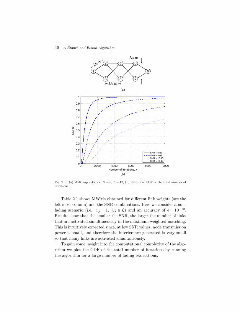
46 A Branch and Bound Algorithm
0 2000 4000 6000 8000 100000
0.1
0.2
0.3
0.4
0.5
0.6
0.7
0.8
0.9
1
Number of iterations, x
(b)
(a)
CD
F(x
)
SNR = 0 dBSNR = 5 dBSNR = 10 dBSNR = 15 dB
Fig. 2.10 (a) Multihop network, N = 8, L = 12; (b) Empirical CDF of the total number ofiterations.
Table 2.1 shows MWMs obtained for different link weights (see theleft most column) and the SNR combinations. Here we consider a non-fading scenario (i.e., cij = 1, i, j ∈ L) and an accuracy of ε = 10−10.Results show that the smaller the SNR, the larger the number of linksthat are activated simultaneously in the maximum weighted matching.This is intuitively expected since, at low SNR values, node transmissionpower is small, and therefore the interference generated is very smallso that many links are activated simultaneously.
To gain some insight into the computational complexity of the algo-rithm we plot the CDF of the total number of iterations by runningthe algorithm for a large number of fading realizations.

2.5 Numerical Examples 47
Tab
le2.
1.M
axim
umw
eigh
ted
mat
chin
gs.
48 A Branch and Bound Algorithm
Figure 2.10(b) shows the empirical CDF plots of the total numberof iterations required to terminate Algorithm 2.1 (or to find theMWM). Plots are drawn for the cases of SNR = 0, 5, 10, and 15 dB,βl = 1 for all l ∈ L, and ε = 10−2. Results show that the smaller theSNR, the smaller the total number of iterations required to find theMWM. For example, in the case of SNR = 0 dB, with probability 0.9,the MWM is found in less than 1500 iterations. However, in the caseof SNR = 5 dB, with the same probability 0.9, the MWM is found inless than 4000 iterations.
2.5.4 Cross-layer Control Policies for NUM
In this section we specifically consider the problem of network utilitymaximization subject to stability constraints [43, sec. 5]. Let us firstrevisit briefly the commodity description of the network. Exogenousdata arrives at the source nodes and they are delivered to the destina-tion nodes over several, possibly multihop, paths. The data is identi-fied by their destinations, i.e., all data with the same destination areconsidered as a single commodity, regardless of their source. We labelthe commodities with integers s = 1, . . . ,S (S ≤ N). For every node,we define Sn ⊆ {1, . . . ,S} as the set of commodities, which can arriveexogenously at node n. The network is time slotted and at each sourcenode, a set of flow controllers decides the amount of each commoditydata admitted in every time slot in the network. Let xs
n(t) denote theamount of data commodity s admitted in the network at node n duringtime slot t. It is assumed that the data that is successfully deliveredto its destination exits the network layer. Associated with each node-commodity pair (n,s)s∈Sn we define a concave and nondecreasing utilityfunction us
n(y), representing the “reward” received by sending data ofcommodity s from node n to node ds at a long term average rate of y
[bits/slot]. Thus, the NUM problem under stability constraints can beformulated as [43, sec. 5]
maximize∑
n∈N∑
s∈Snus
n(ysn)
subject to (ysn)n∈N ,s∈Sn ∈ Λ,
(2.56)
where the variable is (ysn)n∈N ,s∈Sn and Λ represents the network layer
capacity region [43, def. 3.7].

2.5 Numerical Examples 49
An arbitrarily close to optimal solutions for problem (2.56) isachieved by a cross-layer control policy, which consists of solvingthree subproblems: (1) flow control, (2) next-hop routing and in-nodescheduling, and (3) RA, during each time slot [43]. The RA subproblemexactly resembles the WSRMax problem (2.2), where the weights aregiven by the maximum differential backlogs of network links [43]. Here,we implement the cross-layer control algorithm in [43] and, in the thirdstep, we use Algorithm 2.1 to solve the RA subproblem. The cross-layer control algorithm is simulated for at least T = 10,000 time slots,and the average rates xs
n are computed by averaging the last t0 = 3000time slots, i.e., xs
n = 1/t0∑T
t=T−t0xs
n(t). We assume that the rates cor-responding to all node-commodity pairs (n,s)s∈Sn ,n ∈ N are subjectto proportional fairness, and therefore we select the utility functionsus
n(y) = loge(y). For a detailed description of the cross-layer controlpolicy [43] the reader may refer to Section 3.1.2.
Two fully connected multihop wireless network setups, as shownin Figure 2.11 are considered, where all nodes have multipacket trans-mit/receieve capability and no node can transmit and receive simulta-neously. Each of the networks consist of four nodes (i.e., N = 4) andtwo commodities, which arrive exogenously at source nodes. In the caseof the first network setup, shown in Figure 2.11(a), commodity 1 arrivesexogenously at node 1, and is intended for node 4; commodity 2 arrivesexogenously at node 4, and is intended for node 1. Nodes are located ina square grid such that the horizontal and the vertical distance betweenadjacent nodes are D0 meters [m]. In the case of the second network
Fig. 2.11 (a) Multihop network 1, N = 4, fully connected, S = 2; (b) Multihop network 2,N = 4, fully connected, S = 2.

50 A Branch and Bound Algorithm
setup, shown in Figure 2.11(b), commodity 1 arrives exogenously atnode 1, and is intended for node 2; commodity 2 arrives exogenouslyat node 2, and is intended for node 3. Nodes are located such thatthree of them form an equilateral triangle and the fourth one is locatedat its center [see Figure 2.11(b)]. It is assumed that the distance fromthe middle node to any other is D0 m. The channel power gains aregiven by (2.54) and SNR operating point is given by (2.55). We setD0/d0 = 10 and η = 4 in the following simulation.
Figure 2.12 shows the dependence of the average network layer sum-rate on the SNR for the considered network setups. As a reference, wefirst consider a suboptimal and more restrictive RA policy, where onlyone link can be activated during each time slot. This policy is calledbase line single link activation (BLSLA); BLSLA policy consists of acti-vating, during each time slot, only the link that achieves the maximumweighted rate. Other suboptimal RA policy is based on CGP algorithm(see Section 2.5.2). Specifically, we use two initialization methods forCGP algorithm: (1) the initial γl, l ∈ L is found according to (2.30)by using BLSLA power allocation, (2) the uniform initialization, asdiscussed in Section 2.5.2.
Results show that the gains obtained by using Algorithm 2.1 arealways larger compared to other suboptimal methods. The relativegains achieved by Algorithm 2.1 in the case of network setup 1[Figure 2.12(a)] are more significant than in the case of networksetup 2 [Figure 2.12(b)]. Results further show that, the suboptimalCGP algorithm is very sensitive to initialization. For example, in thecase of uniform initialization, CGP algorithm performs extremelypoorly compared to the case of BLSLA based initialization. Moreover,in the case of BLSLA based initialization, the suboptimal CGPalgorithm can not perform beyond the limits that are achieved bysimple BLSLA RA policy.
2.5.5 Achievable Rate Regions in SinglecastWireless Networks
In this section we illustrate how Algorithm 2.1 can be used to find theachievable rate region in singlecast wireless networks. Recall that weconsider the case where all receiver nodes perform singleuser detection,

2.5 Numerical Examples 51
0 2 4 6 8 10 12 14 160
0.5
1
1.5
2
2.5
3
3.5
4
SNR [dB]
Ave
rage
net
wor
k la
yer
sum
−ra
te [b
its/s
lot]
Alg. 2.1BLSLACGP alg., BLSLA init.CGP alg., uniform init.
0 2 4 6 8 10 12 14 160
0.5
1
1.5
2
2.5
3
3.5
4
SNR [dB]
Ave
rage
net
wor
k la
yer
sum
−ra
te [b
its/s
lot]
Alg. 2.1BLSLACGP alg., BLSLA init.CGP alg., uniform init.
Fig. 2.12 (a) Dependence of average network layer sum-rate on SNR for network 1;(b) Dependence of average network layer sum-rate on SNR for network 2.
and therefore the achievable rate regions we are referring to are differentfrom the information theoretic capacity regions [1, 126, 137]. Note thatthe information theoretic capacity region is not known, even in thesimple case of two interfering links [36].

52 A Branch and Bound Algorithm
To facilitate the graphical illustration, we consider a simple bipartitesinglecast network of degree 1, as shown in Figure 2.5(b). The channelpower gains are given by (2.52) and the SNR operating point is givenby (2.53).
We start by defining the directly achievable rate region, the instan-taneous rate region, and the average rate region for singlecast wirelessnetworks. Let RDIR−SC(µ, C(t),pmax
1 ,pmax2 ) denote the directly achiev-
able rate region for a given interference coupling index µ, a given fadingrealization9
C(t) = {c11(t), c12(t), c22(t), c21(t)}, (2.57)
and maximum node transmission power pmax1 and pmax
2 , i.e.,
RDIR−SC(µ, C(t),pmax1 ,pmax
2 )
=
(R1,R2)
∣∣∣∣∣∣∣∣∣∣∣
R1 ≤ log(
1 +c11(t)p1
σ2 + µc21(t)p2
)
R2 ≤ log(
1 +c22(t)p2
σ2 + µc12(t)p1
)0 ≤ p1 ≤ pmax
1 , 0 ≤ p2 ≤ pmax2
. (2.58)
By invoking a time sharing argument, one can obtain the instan-taneous rate region RINS−SC(µ, C(t),pmax
1 ,pmax2 ); the convex hull of
RDIR−SC(µ, C(t),pmax1 ,pmax
2 ). That is,
RINS−SC(µ, C(t),pmax1 ,pmax
2 ) = conv{
RDIR−SC(µ, C(t),pmax1 ,pmax
2 )}
,
where conv{R} denotes the convex hull of the set R. As noted in [48],since the instantaneous rate region RINS−SC(µ, C(t),pmax
1 ,pmax2 ) is con-
vex, any boundary point of the rate region can be obtained by using thesolution of an optimization problem in the form of (2.2) with β1 = α,β2 = (1 − α) for some α ∈ [0,1].
Finally, we define the average rate region RAVE−SC(µ,pmax1 ,pmax
2 )for a given interference coupling index µ and a maximum node
9 The argument t is used to indicate the fading realization index.
2.5 Numerical Examples 53
transmission power pmax1 and pmax
2 as RAVE−SC(µ,pmax1 ,pmax
2 ) =1T
∑Tt=1 RINS−SC(µ, C(t),pmax
1 ,pmax2 ), where addition and scalar multi-
plication of sets is used.10 The nonnegative integer T is the total numberof fading realizations we used in averaging. Note that, any boundarypoint (Rb
1 ,Rb2) of RAVE−SC(µ,pmax
1 ,pmax2 ) is obtained by using the fol-
lowing steps for some α ∈ [0,1]: (1) solve problem (2.2) with β1 = α
and β2 = 1 − α for T fading realizations, (2) for each fading realizationt ∈ {1, . . . , T}, evaluate the rate of link 1 and 2 denoted by r1(t), r2(t)according to (2.1), and (3) average r1(t) and r2(t) over all T fadingrealizations to obtain Rb
1 = 1T
∑Tt=1 r1(t) and Rb
2 = 1T
∑Tt=1 r2(t).
Figure 2.13(a) shows RINS−SC(µ, C(t),pmax1 ,pmax
2 ), the instantaneousrate regions for different values of µ and for an arbitrary chosen fad-ing realization in the case of SNR = 15 dB. Specifically, the fadingcoefficients are c11(t) = 0.4185, c12(t) = 0.3421, c22(t) = 0.3700, andc21(t) = 1.299. As a reference, we also plot the directly achievablerate regions RDIR−SC(µ, C(t),pmax
1 ,pmax2 ) for all the scenarios con-
sidered. Note that the problem of finding any boundary point ofRDIR−SC(µ, C(t),pmax
1 ,pmax2 ) can be easily cast as a GP, or as a problem
of the form (2.35). Results show that the smaller the µ, the larger therate regions. This is intuitively explained by noting that the smallerthe µ, the smaller the interference coefficients, gij between links, andtherefore the higher the rates. When µ ≥ 0.2, the directly achievablerate regions become nonconvex, whereas the instantaneous rate regionis a triangle referred to as time division multiple access (TDMA) rateregion, obtained by time sharing between the maximum rates of R1
and R2. Moreover, when µ < 0.2, the instantaneous rate region expandsbeyond the TDMA rate region and for µ ≤ 0.01, the directly achievablerate region almost overlaps with the instantaneous rate region.
Figure 2.13(b) shows the average rate region RAVE−SC
(µ,pmax1 ,pmax
2 ) for different values of µ in the case of SNR = 15dB. As a reference, we also plot the region obtained by using CGPalgorithm to problem (2.2). Results show that the region obtainedby CGP algorithm is always worse than the average rate region. The
10 For vector sets A1 and A2 and scalars α1,α2, the set α1A1 + α2A2 is defined as {α1a1 +α2a2 |a1 ∈ A1,a2 ∈ A2} [22, p. 38].

54 A Branch and Bound Algorithm
0 0.5 1 1.5 2 2.5 3 3.5 40
0.5
1
1.5
2
2.5
3
3.5
4
R1 [bits/s/Hz]
R2
[bits
/s/H
z]
instantaneous rate regiondirectly achievable rate region
µ ≥ 0.2
µ = 0.15
µ = 0.2
µ = 0.3
µ = 0.5
µ = 1
C2
C1
µ = 0.01,rate regions almost overlap
µ = 0.02rate regions almost overlap
µ = 0rate regions almost overlap
0 0.5 1 1.5 2 2.5 3 3.5 4 4.50
0.5
1
1.5
2
2.5
3
3.5
4
4.5
R1 [bits/s/Hz]
(a)
(b)
R2
[bits
/s/H
z]
average rate regionregion obtained by CGP alg.
C2
C1
µ = 1
µ = 0.1
µ = 0.05
µ = 0.02
µ = 0
Fig. 2.13 Rate regions: (a) Directly achievable and instantaneous rate regions; (b) Averagerate regions.
gap in performance is more pronounced in the case of larger valuesof µ. Note that, even in the case of µ = 1, the average rate region isbounded by a concave function with end points C1 and C2, althoughthe corresponding instantaneous rate regions used in the averaging

2.5 Numerical Examples 55
are triangles [see Figure 2.13(a)] in general. This phenomenon isdue to the property of the set addition used in the definition ofRAVE−SC(µ,pmax
1 ,pmax2 ). Results also show that the smaller the µ, the
larger the average rate region.
2.5.6 Achievable Rate Regions in MulticastWireless Networks
We finally show the applicability of Algorithm 2.1 for finding the rateregions in a multicast wireless networks. A multicast with only twomulticast transmissions [see Figure 2.14(a)] is considered for the sake
0 1 2 3 4 50
0.5
1
1.5
2
2.5
3
3.5
4
R1 [bits/s/Hz]
(b)
(a)
R2
[bits
/s/H
z]
SNR = 0 dBSNR = 5 dBSNR = 10 dBSNR = 15 dBSNR = 20 dB
[1 1]T
Fig. 2.14 (a) Multicast network, T = {1,2}, M1 = 1, M2 = 1, O1(1) = {1,2}, O1(2) ={3,4}; (b) Average rate region.

56 A Branch and Bound Algorithm
of graphical illustration of the rate regions. Node 1 has common infor-mation to send to nodes 3 and 4, whereas node 2 has common informa-tion to send to nodes 3 and 5. We assume that node 3 has multipacketreceiver capability. The channel power gains are given by (2.54) andSNR operating point is given by (2.55). Moreover, we set D0/d0 = 10and η = 4.
As in the case of singlecast wireless networks, we first define thedirectly achievable rate region, instantaneous rate region, and the aver-age rate region for multicast wireless networks. Particularized to thenetwork setup in Figure 2.14(a), for a given set of interference coeffi-cients/power gains
G(t) = {g11(t),g22(t),g33(t),g44(t),g14(t),g32(t)} (2.59)
and maximum node transmission power pmax1 and pmax
2 , the instanta-neous rate region RINS−MC(G(t),pmax
1 ,pmax2 ) is defined as
RINS−MC(G(t),pmax1 ,pmax
2 ) = conv{
RDIR−MC(G(t),pmax1 ,pmax
2 )}
,
(2.60)where RDIR−MC(G(t),pmax
1 ,pmax2 ) denotes the directly achievable rate
region for multicast wireless networks, i.e.,
RDIR−MC(G(t),pmax1 ,pmax
2 )
=
(R1,R2)
∣∣∣∣∣∣∣∣∣∣∣∣∣∣∣∣∣∣∣∣∣∣
R1 ≤ log(
1 +g11(t)p1
1
σ2 + g33(t)p12
)
R1 ≤ log(
1 +g22(t)p1
1
σ2 + g32(t)p12
)
R2 ≤ log(
1 +g33(t)p1
2
σ2 + g11(t)p11
)
R2 ≤ log(
1 +g44(t)p1
2
σ2 + g14(t)p11
)0 ≤ p1
1 ≤ pmax1 , 0 ≤ p1
2 ≤ pmax2
. (2.61)
Finally, for a given maximum node transmission power pmax1 and
pmax2 , the average rate region RAVE−MC(pmax
1 ,pmax2 ) is defined as
RAVE−MC(pmax1 ,pmax
2 ) = 1T
∑Tt=1 RINS−MC(G(t),pmax
1 ,pmax2 ).

2.6 Summary and Discussion 57
Figure 2.14(b) shows the average multicast rate region for differentSNR values. Results show that, when the weights associated with ratesR1 and R2 are same, the resulting R1 is always greater than R2. Forexample, in the case of SNR = 20 dB, we have R1 = 3.71 bits/sec/Hzand R2 = 1.50 bits/sec/Hz. Roughly speaking, this observation can beexplained as follows: R1 is determined by the rate of link 2 (the weakestof link 1 and link 2), R2 is determined by the rate of link 3 (the weakestof link 3 and link 4) and rate of link 2 is larger than that of link 3 dueto path losses.
2.6 Summary and Discussion
We considered the general WSRMax problem for a set of interferinglinks. In fact, this problem is NP-hard. A solution method, based onthe branch and bound technique, was presented for solving the noncon-vex WSRMax problem globally with an optimality certificate. Efficientand analytic bounds were given and their impact on convergence wasnumerically evaluated. The convergence speed of the given algorithmcan be substantially increased by improving the lower bound, whilst thetightness of the upper bound has a much reduced impact. Numericalresults showed that the algorithm converges fairly fast in all consid-ered setups. Nevertheless, since the problem is NP-hard, the worst casecomplexity can be exponential in the number of variables.
The considered link-interference model is fairly general so thatit can model a wide range of network topologies with various nodecapabilities, such as single- or multipacket transmission (or reception)and simultaneous transmission and reception. Unlike other branch andbound based solution methods for WSRMax, the method given doesnot require the problem to be convertible into a DC (difference ofconvex functions) problem. Therefore, the given method applies toa broader class of WSRMax problems (e.g., WSRMax in multicastwireless networks). Moreover, the method can also be used to max-imize any system performance metric that can be expressed as aLipschitz continuous and increasing function of SINR values and isnot restricted to WSRMax. Given its generality, the algorithm can beadapted to address a wide range of network control and optimization

58 A Branch and Bound Algorithm
problems. Performance benchmarks for various network topologies canbe obtained by back-substituting it into any network design methodwhich relies on WSRMax. Several applications, including cross-layernetwork utility maximization and maximum weighted link schedulingfor multihop wireless networks, as well as finding achievable rate regionsfor singlecast/multicast wireless networks, have been presented. Sincethere are a number of suboptimal but low-complex algorithms are typ-ically used in practice, the algorithm can also be used for evaluatingtheir performance loss.

3Low Complexity Algorithms
In this section we first present efficient, low-complexity algorithms forthe WSRMax problem in multicommodity, multichannel wireless net-works by using homotopy methods [4] and complementary geometricprogram (or CGP) [6]. The considered problem formulation is fairlygeneral and it allows frequency reuse by activating multiple links in thesame channel simultaneously. Here, the interference is solely resolvedvia power control. Furthermore, the formulation allows the possibil-ity of exploiting multichannel diversity via dynamic power allocationacross the available channels. The gains that can be achieved at upperlayers in terms of end-to-end rates and network congestion are quanti-tatively analyzed by incorporating the algorithms within Neely’s cross-layer utility maximization framework [43, 80].
The algorithm based on homotopy methods, also handles the self-interference problem in such a way that the combinatorial nature ofthe problem is circumvented. Here the imperfect self interference can-celation is modeled as a variable power gain from the transmitter tothe receiver at all nodes. This simple model gives insight into thebehavior of different network topologies when self interference cancela-tion is employed in network nodes. A similar approach can be used ina straightforward manner to model a wide range of network topologies
59
60 Low Complexity Algorithms
with various node capabilities as well, for example, singlepacket trans-mission, singlepacket reception, and many others. The method can alsobe used to find the required level of accuracy for the self interferencecancelation such that certain gains are achieved at the network layer.In addition, it provides a simple mechanism to evaluate the impact ofscaling the distance between network nodes on the accuracy level of theself interference cancelation. Thus, from a network design perspective,the method presented here can be very useful.
Recall that WSRMax problem is NP-hard and one has to rely onexponentially complex global optimization techniques [5, 16, 52] toobtain the optimal solution. Nevertheless, the numerical results showthat the algorithms presented in this section perform close to globaloptimization methods. We further test the algorithms by carryingthem out on large-scale problems, where global optimization methods[28, 97, 129, 135, 139] cannot be used, due to prohibitive computa-tional complexity. Results show that the given algorithms can providesignificant gains at the network layer, in terms of end-to-end rates andnetwork congestion, by exploiting efficiently the available multichanneldiversity. We also evaluate the potential gains achievable at the net-work layer when the network nodes employ self interference cancelationtechniques with different degrees of accuracy.
Finally, we consider different receiver capabilities and examine theeffect of the use of multiuser detectors.
3.1 System Model and Problem Formulation
3.1.1 Network Model
The wireless network consists of a collection of nodes that can send,receive and relay data across wireless links. The set of all nodesis denoted by N and we label the nodes with the integer valuesn = 1, . . . ,N . A wireless link is represented as an ordered pair (i, j)of distinct nodes. The set of links is denoted by L and we label thelinks with the integer values l = 1, . . . ,L. We define tran(l) as the trans-mitter node of link l, and rec(l) as the receiver node of link l. Theexistence of a link l ∈ L implies that direct transmission is possiblefrom tran(l) to rec(l). We assume that each node can be equipped with

3.1 System Model and Problem Formulation 61
multiple transceivers, that is, any node can simultaneously transmit to,or receive from, multiple nodes. We define O(n) as the set of links thatare outgoing from node n, and I(n) as the set of links that are incom-ing to node n. Furthermore, we denote the set of transmitter nodes byT and the set of receiver nodes by R, i.e., T = {n ∈ N|O(n) �= ∅} andR = {n ∈ N|I(n) �= ∅}.
The network is assumed to operate in slotted time with slots normal-ized to integer values t ∈ {1,2,3, . . .}. All wireless links are sharing a setC of orthogonal channels, labeled with integers c = 1, . . . ,C. When thereare many channels which fade independently, at any one time there is ahigh probability that one of the channels will be strong. Thus, the mainmotivation for considering multiple channels is exploitation of the diver-sity that results from unequal links’ behavior across a given wide band.
Let hijc(t) denote the channel gain from the transmitter of link i
to the receiver of link j in channel c during time slot t. We assumethat hijc(t) are constant for the duration of a time slot and are inde-pendent and identically distributed over the time slots, links as wellas over the channels. Let giic(t) represent the power gain of link i inchannel c during time slot t, i.e., giic(t) = |hiic(t)|2 (see Figure 3.1). Forany pair of distinct links i �= j, we denote the interference coefficientfrom link i to link j in channel c by gijc(t). In the case of nonadjacentlinks (i.e., links i and j do not have common nodes), gijc represents thepower of the interference signal at the receiver node of link j in chan-nel c when one unit of power is allocated to the transmitter node oflink i in channel c, i.e., gijc = |hijc|2. When links i and j are adjacent,the value of gijc represents the power gain in channel c within thesame node from its transmitter to its receiver, and is referred to as the
Fig. 3.1 Choosing the value of interference coefficients, i.e., gij for i �= j and link powergains, i.e., gii and gjj (channel index c and time index t are omitted for clarity): A = {(i, j)},gij = g, gji = |hji|2, gii = |hii|2, and gjj = |hjj |2.

62 Low Complexity Algorithms
self-interference coefficient (see Figure 3.1). For notational conveniencelet A denote the set of all link pairs (i, j) such that links i and j areadjacent. In other words, A represents the set of all link pairs (i, j) forwhich the transmitter of link i and the receiver of link j coincide, i.e.,A = {(i, j)i,j∈L| tran(i) = rec(j)} (see Figure 3.1). Specifically, for all(i, j) ∈ A, we set gijc(t) = g to model the residual self-interference gainsafter a certain self interference cancelation technique was employed atthe network’s nodes in channel c, where g ∈ [0,1] is a scalar. We refer tog as the self-interference gain (see Figure 3.1). A value g = 1 means thatno self interference cancelation technique is used and models the verylarge self interference that would affect the incoming links of a node ifit simultaneously transmitted and received in the same channel. On theother hand, a value g = 0 corresponds to a perfect self interference can-celation. Note that, according to relative distances between network’snodes, gijc(t) for all (i, j) ∈ A (i.e., the self-interference coefficients) canbe several orders of magnitude larger than gijc(t) for all (i, j) �∈ A. Theparticular class of network topologies, for which A = ∅ (i.e., T ∩ R = ∅)is referred to as bipartite networks. On the other hand, the class of net-work topologies, for which A �= ∅ (i.e., T ∩ R �= ∅) is referred to asnonbipartite networks. Note that all multihop networks are necessarilynonbipartite.
In every time slot a network controller decides the power and ratesallocated to each link in every channel. We denote the power allocatedto each link l in channel c during time slot t by plc(t). The power alloca-tion is subject to a maximum power constraint
∑c∈C
∑l∈O(n) plc(t) ≤
pmaxn for each node n.
We consider first the case where all receivers perform singleuserdetection, i.e., any receiver decodes each of its intended signals by treat-ing all other interfering signals as noise. Extensions to more advancedmultiuser detection techniques will be addressed in Section 3.3. Supposethat the achievable rate of link l during time slot t is given by
rl(t) =C∑
c=1
Wc log
(1 +
gllc(t)plc(t)NlWc +
∑j �=l gjlc(t)pjc(t)
), (3.1)
where Wc represents the bandwidth of channel c and Nl is the powerspectral density of the noise at the receiver of link l. Note that for

3.1 System Model and Problem Formulation 63
any link l, interference at rec(l)[i.e., the term
∑j �=l gjlc(t)pjc(t)
]is
created by self transmissions[i.e.,
∑j∈O(rec(l)) gjlc(t)pjc(t)
], as well as
by the other node transmissions[i.e.,
∑j∈L\{O(rec(l))∪{l}} gjlc(t)pjc(t)
].
To simplify the presentation, we assume in the sequel that all channelshave equal bandwidths and that the noise power density is the sameat all receivers (i.e., Wc = W for all c ∈ C and Nl = N0 for all l ∈ L).The extension to the case of unequal bandwidths Wc and noise powerspectral densities Nl is straightforward. Let σ2 = N0W denote the noisepower, which is constant for all receivers in all channels. Furthermore,we denote by P(t) ∈ IRL×C
+ the overall power allocation matrix, i.e.,plc(t) = [P(t)]l,c. The use of the Shannon formula for the achievablerate in (3.1) is approximate in the case of finite length packets andis used to avoid the complexity of rate-power dependence in practicalmodulation and coding schemes. This is common practice but it mustbe noted that this is not strictly correct. However, as the packet lengthincreases it is asymptotically correct.
3.1.2 Network Utility Maximization
Exogenous data arrive at the source nodes and they are delivered to thedestination nodes over several, possibly multihop, paths. We identifythe data by their destinations, i.e., all data with the same destinationare considered as a single commodity, regardless of their source. Actu-ally, formulation considered also permits the anycast case, in which anydata exits the network as soon as any of particular destination set ofnodes receives the data successfully. We label the commodities withintegers s = 1, . . . ,S (S ≤ N) and the destination node of commodity s
is denoted by ds. For every node, we define Sn ⊆ {1, . . . ,S} as the setof commodities that can arrive exogenously at node n.
A network utility maximization, or NUM, framework similar to theone given in [43, sec. 5.1] is considered. Specifically, exogenously arriv-ing data is not directly admitted to the network layer. Instead, theexogenous data is first placed in the transport layer storage reser-voirs. To avoid complications that may arise that are extraneous tothe main focus, we assume that all commodities have infinite demandat the transport layer. Nevertheless, the resource allocation (or RA)

64 Low Complexity Algorithms
algorithms given in this section are still applicable when this assump-tion is relaxed. At each source node, a set of flow controllers decides theamount of each commodity data admitted during every time slot in thenetwork. Let xs
n(t) denote the amount of data of commodity s admit-ted in the network at node n during time slot t. At the network layer,each node maintains a set of S internal queues for storing the currentbacklog (or unfinished work) of each commodity. Let qs
n(t) denote thecurrent backlog of commodity s data stored at node n. We formallylet qs
ds(t) = 0, i.e., it is assumed that data, which is successfully deliv-
ered to its destination, exits the network layer. Associated with eachnode-commodity pair (n,s)s∈Sn we define a concave and nondecreasingutility function us
n(y), representing the “reward” received by sendingdata of commodity s from node n to node ds at a long term averagerate of y [bits/slot].
The NUM problem under stability constraints is [43, sec. 5]
maximize∑
n∈N∑
s∈Snus
n(ysn)
subject to (ysn)n∈N ,s∈Sn ∈ Λ,
(3.2)
where the variable is (ysn)n∈N , s∈Sn and Λ represents the network layer
capacity region. In particular, the network layer capacity region Λ isthe closure of the set of all admissible arrival rate vectors that canbe stably supported by the network, considering all possible strategiesfor choosing the control variables that affect routing, scheduling, andresource allocation (including those with perfect knowledge of futureevents) [43, p. 28].
A dynamic cross-layer control algorithm, which achieves a utilitythat is arbitrarily close to the optimal value of problem (3.2), has beenintroduced in [43, sec. 5]. Specifically, the algorithm’s performance canbe characterized as follows:∑
n∈N
∑s∈Sn
usn(y�s
n) − liminfT→∞
∑n∈N
∑s∈Sn
usn
(1T
∑t=1:T
E{xsn(t)}
)≤ B
V, (3.3)
where (y�sn)n∈N ,s∈Sn is the optimal solution of problem (3.2), B > 0 is
a well defined constant, and V > 0 is an algorithm parameter that canbe used to control the tightness of the achieved utility to the optimalvalue [43, sec. 5.2.1]. The details are extraneous to the central objective

3.1 System Model and Problem Formulation 65
of this section. Particularized to the considered network model, in everytime slot t, the algorithm performs the following steps:
Algorithm 3.1 Dynamic cross-layer control algorithm [43, sec. 5.2].
1. Flow control; each node n ∈ N solves the following problem:
maximize∑
s∈SnV us
n(xsn) − xs
nqsn(t)
subject to∑
s∈Snxs
n ≤ Rmaxn , xs
n ≥ 0,(3.4)
where the variable is (xsn)s∈Sn . Set (xs
n(t) = xsn)s∈Sn . The
parameter V > 0 is a chosen parameter that affects the algo-rithm performance [see (3.3)] and Rmax
n > 0 is used to controlthe burstiness of data delivered to the network layer.
2. Routing and in-node scheduling; for each link l, let
βl(t) = maxs
{qstran(l)(t) − qs
rec(l)(t),0}
c�l (t) = argmax
s
{qstran(l)(t) − qs
rec(l)(t),0}.
(3.5)
If βl(t) > 0, the commodity that maximizes the differentialbacklog, i.e., c�
l (t), is selected for potential routing over link l.This is the well known rule of next-hop transmission underthe backpressure algorithm [120].
3. Resource allocation; the power allocation P(t) is given by Pwhose entries plc solve the following problem
maximize∑l∈L
βl(t)∑c∈C
log(
1+gllc(t)plc
σ2+∑j �=l
gjlc(t)pjc
)
subject to∑c∈C
∑l∈O(n)
plc ≤ pmaxn , n ∈ N
plc ≥ 0, l ∈ L, c ∈ C.
(3.6)
Once the optimal power allocation P(t) is determined, com-pute rate allocation rl(t) for all l ∈ L by using (3.1). Theresulting rate rl(t) is offered to the data of commodity c�
l (t).
In the first step, each node n determines the amount of data of com-modity s
(i.e., xs
n(t) for all s ∈ Sn
)that are admitted in the network,
66 Low Complexity Algorithms
based on the current backlogs(i.e., qs
n(t) for all s ∈ Sn
). In the second
step, each node n computes βl and the corresponding commodity c�l (t)
for all l ∈ O(n). The commodity c�l (t) is selected for potential rout-
ing over link l during time slot t. Recall that in-node scheduling refersto selecting the appropriate commodity and it is not to be confusedwith the links scheduling mechanism, which is handled by the RA sub-problem, i.e., step 3. The third step is the most difficult part of Algo-rithm 3.1, which computes the power allocation P(t) in each link l. Ofcourse, the RA subproblem maximizes the sum of weighted rates, i.e.,WSRMax. The solution P(t) determines implicitly the links/channelsthat should be activated in every time slot t. The power allocation P(t)is used to determine rl(t) [see (3.1)] and the resulting link rate rl(t) isoffered to the data of commodity c�
l (t). Since thw main focus residesin problem (3.6), extensive explanations of Algorithm 3.1 are avoided.However, we refer the reader to [43, sec. 5] for more details.
3.2 Algorithm Derivation: CGP and Homotopy Methods
In this section we focus on resource allocation problem (3.6). By usingstandard reformulation techniques, we first show that problem (3.6)is equivalent to a CGP [6]. Then we obtain a successive approxima-tion algorithm for problem (3.6) in bipartite networks. Next we explainthe challenges of the problem in nonbipartite networks (e.g., multihopnetworks), due to the self-interference problem; when a node simulta-neously transmits and receives in the same channel, its incoming linksare affected by very large self interference levels. Finally, we presenta method based on homotopy methods [4], together with CGP, whichcircumvents the aforementioned difficulties.
3.2.1 CGP for WSRMax
Let us denote the negative of the objective function of problem (3.6)by f0
(P). It can be expressed as
f0(P)
= −∑l∈L
∑c∈C
log(
1 +gllcplc
σ2 +∑
j �=l gjlcpjc
)βl
(3.7)
= log∏l∈L
∏c∈C
(1 + γlc
)−βl , (3.8)

3.2 Algorithm Derivation: CGP and Homotopy Methods 67
where the time index t was dropped for the sake of notational simplicity,and γlc represents the SINR of link l in channel c, i.e.,
γlc =gllcplc
σ2 +∑
j �=l gjlcpjc, l ∈ L, c ∈ C. (3.9)
Since log(·) is an increasing function, problem (3.6) can be reformulatedequivalently as
minimize∏
c∈C∏
l∈L(1 + γlc
)−βl
subject to γlc =gllcplc
σ2 +∑
j �=l gjlcpjc, l ∈ L, c ∈ C
∑c∈C
∑l∈O(n) plc ≤ pmax
n , n ∈ N
plc ≥ 0, l ∈ L, c ∈ C,
(3.10)
where the variables are (plc)l∈L,c∈C and (γlc)l∈L,c∈C . Now we considerthe related problem
minimize∏
c∈C∏
l∈L(1 + γlc
)−βl
subject to γlc ≤ gllcplc
σ2 +∑
j �=l gjlcpjc, l ∈ L, c ∈ C∑
c∈C∑
l∈O(n) plc ≤ pmaxn , n ∈ N
plc ≥ 0, l ∈ L, c ∈ C,
(3.11)
with the same variables (plc)l∈L,c∈C and (γlc)l∈L,c∈C . Note that theequality constraints of problem (3.10) have been replaced with inequal-ity constraints. We refer to these inequality constraints as SINR con-straints for simplicity. Since the objective function of problem (3.11) isdecreasing in each γlc, we can guarantee that at any optimal solutionof problem (3.11), the SINR constraints must be active.1 Therefore wesolve problem (3.11) instead of problem (3.10).
1 Otherwise, we can show by contradiction that the current solution is not optimal.

68 Low Complexity Algorithms
Finally, by introducing the auxiliary variables vlc ≤ 1 + γlc and rear-ranging the terms, problem (3.6) can be further reformulated as
minimize∏
c∈C∏
l∈L v−βllc
subject to vlc ≤ 1 + γlc, l ∈ L, c ∈ Cσ2g−1
llc p−1lc γlc +
∑j �=l g
−1llc gjlcpjcp
−1lc γlc ≤ 1, l ∈ L, c ∈ C∑
c∈C∑
l∈O(n)(pmax
n
)−1plc ≤ 1, n ∈ N
plc ≥ 0, l ∈ L, c ∈ C,(3.12)
where the variables are (plc)l∈L,c∈C , (γlc)l∈L,c∈C , and (vlc)l∈L,c∈C . Prob-lem (3.12) is a CGP.
3.2.2 Successive Approximation Algorithmfor WSRMax in Bipartite Networks
In this section we consider the case of bipartite networks. Recall fromSection 3.1.1 that for such networks we have A = ∅. By inspectingproblem (3.12), we notice the following: (1) the objective is a mono-mial function [20, sec. 2.1], (2) the right-hand side (RHS) terms of thefirst inequality constraints (i.e., 1 + γlc) are posynomial functions, and(3) the left-hand side terms of all the inequality constraints are eithermonomial or posynomial functions. Note that if the RHS terms of thefirst inequality constraints were monomial functions (instead of posyno-mial ones), problem (3.12) would become a geometric program (or GP)in standard form. GPs can be reformulated as convex problems andthey can be solved very efficiently, even for large scale problems [20,sec. 2.5]. These observations suggest that by starting from an initialpoint, one can search for a close local optimum by solving a sequenceof GPs, which locally approximate the original problem (3.12). At eachstep, the GP is obtained by replacing the posynomial functions in theRHS of the first inequality constraints with their best local monomialapproximations near the the solution obtained at the previous step. Thesolution methods achieved by monomial approximations [6, 20] can beconsidered as a subset of a broader class of mathematical optimizationproblems, known in mathematical literature as inner approximationalgorithms for nonconvex problems [77]. The monomial approximation

3.2 Algorithm Derivation: CGP and Homotopy Methods 69
for the RHS terms of the first inequality constraints in problem (3.12)is described in the following lemma.
Lemma 3.1. Consider the function s(γ) = 1 + γ, γ > 0. Let m(γ) =kγa, γ > 0, be a monomial function used to approximate s(γ) near anarbitrary point γ > 0. Then,
1. the parameters a and k of the best monomial local approxi-mation are given by
a = γ(1 + γ)−1, k = γ−a(1 + γ). (3.13)
2. s(γ) ≥ m(γ) for all γ > 0.
Proof. To show the first part we note the following: the monomial func-tion m is the best local approximation of s near the point γ if
m(γ) = s(γ), m′(γ) = s′(γ). (3.14)
By replacing the expressions of m and s in (3.14) we obtain the follow-ing system of equations: {
kγa = 1 + γ
kaγa−1 = 1,(3.15)
which has the solution given by (3.13).The second part follows from (3.14) and noting that s(γ) is affine
and m(γ) is concave on IR+; concavity of m(γ) follows from the factthat k > 0 and 0 < a < 1 [22, sec. 3.1.5].
The approximation given in Lemma 3.1 turns out to be equivalentto the lower bound approximation used in [94, sec. III-B] for dynamicspectrum management in digital subscriber lines.
Let us now turn to the GP obtained by using the local approxi-mation given by Lemma 3.1. The posynomial functions 1 + γlc of thefirst inequality constraints of problem (3.12) are approximated near thepoint γlc. Consequently the approximate inequality constraints become
vlc ≤ klcγalclc , l ∈ L, c ∈ C, (3.16)

70 Low Complexity Algorithms
where alc and klc have the forms given in (3.13). Since the objectivefunction of problem (3.12) is a decreasing function of vlc, l ∈ L, c ∈ C,it can be easily verified that all of these modified inequality constraintswill be active at the solution of the GP. Therefore, we can eliminatethe auxiliary variables vlc and rewrite the objective function of prob-lem (3.12) as
∏l∈L
∏c∈C
v−βllc =
∏l∈L
∏c∈C
k−βllc γ−βlalc
lc = K∏l∈L
∏c∈C
γlc−βl
γlc1+γlc , (3.17)
where K is a multiplicative constant which does not affect the problemsolution.
In the following subsections, we examine computationally efficientalgorithms to obtain a suboptimal solution for problem (3.12). Fornotational convenience it is useful to define the overall SINR matri-ces γ, γ ∈ IRL×C
+ as [γ]l,c = γlc and [γ]l,c = γlc, respectively.A very brief outline of the successive approximation algorithm is
as follows. It solves an approximated version of problem (3.12) inevery iteration and the algorithm consists of repeating this step untilconvergence.
The first step initializes the algorithm and an initial feasible SINRguess γ(i) is computed. For bipartite networks, there is no self-interference problem, and a simple uniform power allocation can beused.
The second step solves an equivalent GP approximation of prob-lem (3.12) around the current guess γ(i) [see problem (3.18)]. Notethat the auxiliary variables (vlc)l∈L,c∈C of problem (3.12) are eliminatedand the objective function of problem (3.12) is replaced by using themonomial approximation at γ(i) given in (3.17); K(i) is a multiplicativeconstant which does not influence the solution of problem (3.18). Thesemonomial approximations are sufficiently accurate only in the closervicinity of the current guess γ(i). Therefore, the first set of inequalityconstraints are added to confine the domain of variables γ to a regionaround the current guess γ(i) [18]. The first set of inequality constraintsof problem (3.18) are sometimes called trust region constraints [18, 20],which are not originally introduced in [6]. Therefore, Algorithm 3.2 isa slightly modified version of the solution method proposed in [6]. The

3.2 Algorithm Derivation: CGP and Homotopy Methods 71
Algorithm 3.2 Successive approximation algorithm for WSRMax1. Initialization; given tolerance ε > 0, a feasible power allo-
cation P0. Set i = 1. The initial SINR guess γ(i) is givenby (3.9).
2. Solving the GP:
minimize K(i) ∏
l∈L
∏
c∈Cγlc
−βlγ(i)lc
1+γ(i)lc
subject to α−1γ(i)lc ≤ γlc ≤ αγ
(i)lc , l ∈ L, c ∈ C
σ2g−1llc p−1
lc γlc +∑
j �=l
g−1llc gjlcpjcp
−1lc γlc ≤ 1, l ∈ L, c ∈ C
∑
c∈C
∑
l∈O(n)
(pmax
n
)−1plc ≤ 1, n ∈ N ,
(3.18)
with the variables (plc)l∈L,c∈C and (γlc)l∈L,c∈C . Denote thesolution by(p�
lc)l∈L,c∈C and (γ�lc)l∈L,c∈C .
3. Stopping criterion; if max(l,c)∈L×C∣∣γ�
lc − γ(i)lc
∣∣ ≤ ε STOP; oth-erwise go to step 4.
4. Set i = i + 1,(γ
(i)lc = γ�
lc
)l∈L,c∈C and go to step 2.
parameter α > 1 controls the desired approximation accuracy. However,it also influences the convergence speed of Algorithm 3.2. At everystep, each entry of the current SINR guess γ(i) can be increased ordecreased at most by a factor α. Thus, a value of α close to 1 providesgood accuracy for the monomial approximations at the cost of slowerconvergence speed, while a value much larger than 1 improves the con-vergence speed at the cost of reduced accuracy. In most practical cases,a fixed value α = 1.1 offers a good speed/accuracy tradeoff [20]. Thoughwe have trust region constraints for problem (3.18), it is not mandataryto include those here and Algorithm 3.2 can still be carried out.
The third step checks whether the SINRs (γ�lc)l∈L,c∈C obtained
from the solution of problem (3.18) have been significantly changedcompared to the entries of the current guess γ(i). If there are nosubstantial changes, then the algorithm terminates and the link

72 Low Complexity Algorithms
rate rl(t) =∑C
c=1 W log(1 + γ�lc) is offered to the data of commod-
ity c�l (t) [given by (3.5)]. Otherwise, the solution (γ�
lc)l∈L,c∈C is takenas the current guess and the algorithm repeats steps 2 to 4 untilconvergence.
Note that the auxiliary variables (vlc)l∈L,c∈C were only used toreformulate problem (3.11) as a CGP [6] [i.e., problem (3.12)], butthey do not appear in Algorithm 3.2. In fact, an identical algorithmresults if, at each step, the objective function of problem (3.11) islocally approximated by a monomial function (see [34, lem. 4.2.2]).This alternative derivation, known in optimization literature as signo-mial programming [20]. Careful comparisons reveal that the algorithmrecently proposed in [78, p. 3034] is almost identical to Algorithm 3.2for single channel case with no trust region constraints, i.e., C = 1 andα = ∞.
The convergence of the Algorithm 3.2 to a Kuhn–Tucker solution ofthe original nonconvex problem (3.12) is guaranteed [77, thm. 1], sincethe algorithm falls into the broader class of mathematical optimizationproblems, inner approximation algorithms for nonconvex problems [77].
One interesting and important remark is that the objective functionof the approximated problem (3.18) in each iteration i yields a upperbound on the objective function of the original problem (3.11), i.e.,
K(i) ∏l∈L
∏c∈C
γlc
−βlγ(i)lc
1+γ(i)lc ≥
∏l∈L
∏c∈C
(1 + γlc
)−βl (3.19)
for (γlc > 0)l∈L, c∈C , with equality when γ = γ(i). This follows directlyfrom the second statement of Lemma 3.1. By using (3.19), we canshow immediately that Algorithm 3.2 is monotonically decreasing; themonotonicity is established by the following theorem.
Theorem 3.2. Let i and i + 1 be any consecutive iterations of Algo-rithm 3.2 and γ(i) and γ(i+1) be the SINR guesses at the beginning ofeach iteration respectively. Then
∏l∈L
∏c∈C
(1 + γ
(i)lc
)−βl
≥∏l∈L
∏c∈C
(1 + γ
(i+1)lc
)−βl
. (3.20)

3.2 Algorithm Derivation: CGP and Homotopy Methods 73
Proof. To show this we write the following relations:
∏l∈L
∏c∈C
(1 + γ
(i)lc
)−βl
= K(i) ∏l∈L
∏c∈C
(γ
(i)lc
)−βlγ(i)lc
1+γ(i)lc (3.21)
≥ K(i) ∏l∈L
∏c∈C
(γ
(i+1)lc
)−βlγ(i)lc
1+γ(i)lc (3.22)
≥∏l∈L
∏c∈C
(1 + γ
(i+1)lc
)−βl
, (3.23)
where (3.21) follows from (3.19), (3.22) follows since γ(i+1) is the solu-tion of problem (3.18), and (3.23) follows again from (3.19).
Therefore we see immediately that Algorithm 3.2 always yields asolution, which is at least as good as the one in the previous iteration.This is important in the context of practical implementations, sincein practice, one can always stop the algorithm within few iterations,before it terminates.
3.2.3 The Self-interference Problemin Nonbipartite Networks
Let us now consider the nonbipartite networks; networks for whichA �= ∅. In other words, the set of nodes cannot be divided into twodistinct subsets, T and R, i.e., T ∩ R �= ∅ (e.g., multihop wirelessnetworks). For example see Figures 3.1 and 3.2. For such networktopologies, there is the self-interference problem and, consequently,the WSRMax problem must also cope with the self-interference prob-lem. The difficulty comes from that the self-interference gains g2 cantypically be a few orders of magnitude larger than the power gainsbetween distinct network nodes {gjjc}j∈L, for example, when there isno self interference cancelation. Therefore there can be a huge imbal-ance between some entries of {gijc}i,j∈L, especially when g is large.Roughly speaking, this can destroy the smoothness of the functionsassociated with the WSRMax problem [e.g., the objective function of
2 Recall that gijc = g for all (i, j) ∈ A.

74 Low Complexity Algorithms
Fig. 3.2 Two node network (channel index c and time index t are omitted for clarity):A = {(1,2), (2,1)}, g12 = 1, g21 = 1, g11 = |h11|2, and g22 = |h22|2.
problem (3.6)] and can ruin the reliability and the efficiency of Algo-rithm 3.2 that solves it, at least suboptimally. In other words, there canbe many highly suboptimal Kuhn–Tucker solutions for problem (3.12)at which Algorithm 3.2 can terminate by returning an undesirable sub-optimal solution. Moreover, the SINR values at the incoming links of anode that simultaneously transmits in the same channel are very smalland the convergence of Algorithm 3.2 can be very slow if it starts withan initial SINR guess γ containing entries with nearly zero values.Therefore, the direct application of Algorithm 3.2 can perform verypoorly and further improvements are necessary.
A standard way to deal with the self-interference problem consistsof adding a supplementary combinatorial constraint into the WSRMaxproblem that does not allow any node in the network to transmit andreceive simultaneously in the same channel [13, 14, 46]. We will refer toa power allocation, which satisfies this constraint as admissible. Notethat this approach would require solving a power optimization problem(by using Algorithm 3.2) for each possible subset of links that can besimultaneously activated. This results in a combinatorial nature for theWSRMax problem in the case of nonbipartite networks [9, 25, 26, 62,68, 112, 138]. Of course, since the complexity of this approach growsexponentially with the number of links and number of channels, thissolution method becomes quickly impractical.
3.2.4 Successive Approximation Algorithm for WSRMax inNonbipartite Networks: A Homotopy Method
To avoid difficulties pointed out in Section 3.2.3, we present an algo-rithm inspired from homotopy methods [4] that can be traced back tolate 80s; see [63] and the references therein. In fact, the well known
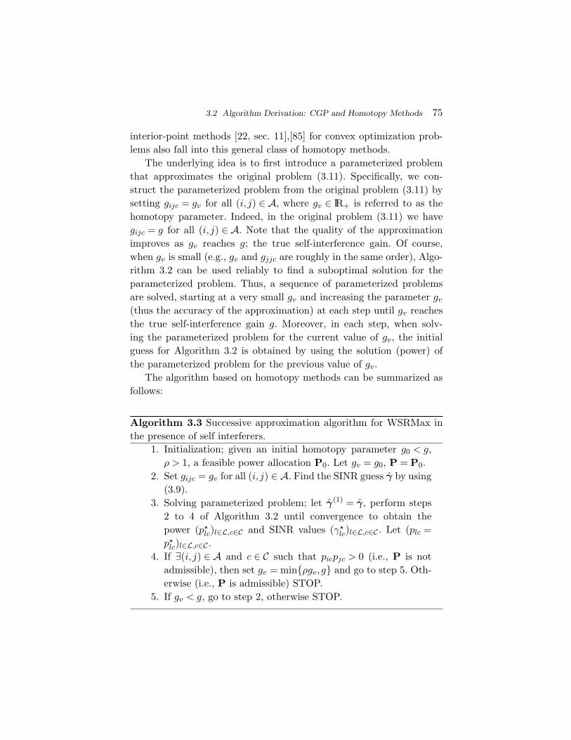
3.2 Algorithm Derivation: CGP and Homotopy Methods 75
interior-point methods [22, sec. 11],[85] for convex optimization prob-lems also fall into this general class of homotopy methods.
The underlying idea is to first introduce a parameterized problemthat approximates the original problem (3.11). Specifically, we con-struct the parameterized problem from the original problem (3.11) bysetting gijc = gv for all (i, j) ∈ A, where gv ∈ IR+ is referred to as thehomotopy parameter. Indeed, in the original problem (3.11) we havegijc = g for all (i, j) ∈ A. Note that the quality of the approximationimproves as gv reaches g; the true self-interference gain. Of course,when gv is small (e.g., gv and gjjc are roughly in the same order), Algo-rithm 3.2 can be used reliably to find a suboptimal solution for theparameterized problem. Thus, a sequence of parameterized problemsare solved, starting at a very small gv and increasing the parameter gv
(thus the accuracy of the approximation) at each step until gv reachesthe true self-interference gain g. Moreover, in each step, when solv-ing the parameterized problem for the current value of gv, the initialguess for Algorithm 3.2 is obtained by using the solution (power) ofthe parameterized problem for the previous value of gv.
The algorithm based on homotopy methods can be summarized asfollows:
Algorithm 3.3 Successive approximation algorithm for WSRMax inthe presence of self interferers.
1. Initialization; given an initial homotopy parameter g0 < g,ρ > 1, a feasible power allocation P0. Let gv = g0, P = P0.
2. Set gijc = gv for all (i, j) ∈ A. Find the SINR guess γ by using(3.9).
3. Solving parameterized problem; let γ(1) = γ, perform steps2 to 4 of Algorithm 3.2 until convergence to obtain thepower (p�
lc)l∈L,c∈C and SINR values (γ�lc)l∈L,c∈C . Let (plc =
p�lc)l∈L,c∈C .
4. If ∃(i, j) ∈ A and c ∈ C such that picpjc > 0 (i.e., P is notadmissible), then set gv = min{ρgv,g} and go to step 5. Oth-erwise (i.e., P is admissible) STOP.
5. If gv < g, go to step 2, otherwise STOP.
76 Low Complexity Algorithms
The first step initializes the algorithm; the homotopy parameter gv
is initialized by g0, where g0 is chosen in the same range of values asthe power gains between distinct nodes. Specifically, in the simulationswe select g0 = maxj∈L,c∈C{gjjc}. Step 2 updates the problem data forthe parameterized problem and a feasible SINR guess is computed. Thethird step finds a suboptimal solution for the parameterized problem.The algorithm terminates in step 4 if P is admissible (thus none ofnodes in the network are transmitting and receiving simultaneously inthe same channel). On the other hand, if P is not admissible, then thehomotopy parameter gv is increased. If gv reaches its extreme allowedvalue (i.e., the actual self-interference gain value of g), the algorithmterminates. Otherwise (i.e., gv < g), it returns to step 2 and continues.Terminating Algorithm 3.3 if the solution is admissible is intuitivelyobvious for the following reason. The data associated with the param-eterized problem that is solved in step 3 of Algorithm 3.3 becomesindependent of the homotopy parameter gv, and therefore a furtherincrease in gv after having an admissible solution has no effect on theresults. Computational experience suggests that Algorithm 3.3 yieldsan admissible solution way before gv reaches value g (e.g., in the caseof no self interference cancelation, i.e., g = 1, an admissible power allo-cation is achieved in about 1−4 iterations with ρ = 2).
Since Algorithm 3.3 runs a finite number of instances of Algo-rithm 3.2, its computational complexity does not increase more thanpolynomially with the problem size. Clearly, Algorithm 3.3 can con-verge to a Kuhn-Tucker solution of the last parameterized problem(the one just before the termination of Algorithm 3.3).
As a specific example to illustrate self interference, consider thesimple network shown in Figure 3.2 and suppose that no self inter-ference cancelation technique is employed at the network’s nodes, i.e.,g = 1. Here, N = 2, L = 2, and C = 1. Note that A = {(1,2),(2,1)}and let β1,β2 �= 0. Suppose that g12 � g22 and g21 � g11, which isoften the case due to path losses. Since the gains g12 = 1 and g21 = 1are very large compared to g22 and g11, for any nonzero power allo-cation p1,p2 = p0 the initial SINR guess γ1, γ2 will have nearly zerovalues. This results in difficulties in using Algorithm 3.2 directly.

3.2 Algorithm Derivation: CGP and Homotopy Methods 77
In Algorithm 3.3 this problem is circumvented by initializing the gainsg12 and g21 by a parameter g0 (e.g., g0 = max{g11,g22}) and executingAlgorithm 3.2 repeatedly, increasing incrementally the parameter gv
until it reaches 1, the true values of g12 and g21.Regarding the complexity of the algorithm we make the following
remarks. The computational complexity of a GP depends on the num-ber of variables and constraints, as well as on the sparsity patternof the problem [20]. Unfortunately, it is difficult to quantify preciselythe sparsity pattern, and therefore a general complexity analysis isnot available. To give a rough idea, let us consider a fully connectednetwork with N = 9 nodes and C = 8 channels. The number of vari-ables in problem (3.18) is 2LC = 1152 and the number of constraintsis 3LC + N = 1737, and it was solved in about 12 seconds on desktopcomputer. The number of iterations depends on the starting point, pmax
n
and channel gains gijc, but typically Algorithm 3.2 required around 100iterations to converge.
Nevertheless, with some slight modifications it is possible to dra-matically decrease the average complexity per iteration, which is veryimportant in the context of practical implementations. Two simplemodifications are as follows:
1. Use a large values for the parameter α in Algorithm 3.2:as we discussed in Section 3.2.2, large α can improve theconvergence speed of Algorithm 3.2 at the cost of reducedaccuracy of the monomial approximation.
2. Eliminate (relatively) insignificant variables; we caneliminate the power variables plc and the associated SINRvariables γlc from problem (3.18) when they have relativelyvery small contributions to the overall objective value of(3.18). Specifically, the exponent term βlγ
(i)lc /
(1 + γ
(i)lc
)in the
objective of (3.18) is evaluated for all l ∈ L, c ∈ C and if
βlγ(i)lc /
(1 + γ
(i)lc
)� max
l∈L,c∈Cβlγ
(i)lc
/(1 + γ
(i)lc
),
then plcs and the associated γlcs are eliminated in succes-sive GPs.

78 Low Complexity Algorithms
3.2.5 Impact of Scaling the Node Distances on theAccuracy of Self Interference Cancelation
Based on a simple exponential path loss model, in this section we dis-cuss the impact of scaling the distance between network nodes on theaccuracy level of the self interference cancelation.
For simplicity, we focus on the single-channel case (i.e., C = 1).Suppose an exponential path loss model, where the channel power gains|hij(t)|2, between distinct nodes are given by
|hij(t)|2 =(
dij
d0
)−η
cij(t). (3.24)
Here dij is the distance from the transmitter of link i to the receiverof link j, d0 is the far field reference distance [64], η is the path lossexponent, and cij(t) are exponentially distributed random variableswith unit mean, independent of the time slots and links. The first termof (3.24) represents the path loss factor and the second term modelsRayleigh small-scale fading.
Suppose pmaxn = pmax
0 for all n ∈ N . For all l ∈ L we define the signal-to-noise ratio (or SNR) of link l as
SNRl =pmax0σ2
(dll
d0
)−η
. (3.25)
It represents the average SNR at rec(l) when tran(l) allocates all itstransmission power to link l and all the other nodes are silent. Let p(t) ∈IRL
+ denote the overall power allocation matrix, i.e., pl(t) = [p(t)]l (notethat the channel index is dropped for simplicity, since C = 1).
Let us consider a network that is obtained from another one, byscaling the distance between distinct nodes and the maximum nodetransmission power such that all link’s SNRs [see (3.25)] are conserved.In the sequel, we show that, in order to preserve the achievable rateregion, the accuracy level of the self interference cancelation techniquesmust also be scaled appropriately.
We start by defining two matrices, which will be useful for laterreference. Let D ∈ IRL×L
+ denote the node distance matrix defined as[D]i,j = dij and G(t) ∈ IRL×L
+ denote the interference coefficient andthe power gain matrix during time slot t, defined as [G(t)]i,j = gij(t).

3.2 Algorithm Derivation: CGP and Homotopy Methods 79
The achievable rate region with singleuser detection at receivers fora given G(t) and a maximum node transmission power pmax
0 can beexpressed as
R(G(t),pmax0 ) =
(rl)l∈L
∣∣∣∣∣∣∣∣∣∣rl ≤ log
(1 +
gll(t)pl
σ2 +∑
j �=l gjl(t)pj
), l∈L∑
l∈O(n) pl ≤ pmax0 , n∈N
pl ≥ 0, l∈L
.
(3.26)
From (3.26), it follows that if the matrix G(t) is scaled by a factor of1/κ, and the maximum node transmission power pmax
0 is scaled by afactor of κ, then the achievable rate region is unchanged, i.e.,
R(G(t),pmax0 ) = R(G(t)/κ,κpmax
0 ). (3.27)
Let κ = θη. According to the exponential path loss model given in(3.24), the scaling of G(t) by a factor of 1/κ (or 1/θη) is equivalentto the scaling of node distance matrix D by a factor of θ and the scal-ing of self-interference gains g by a factor of 1/θη. Therefore, with aslight abuse of notation, we rewrite (3.27) as
R(D,g,pmax0 ) = R(θD,g/θη,θηpmax
0 ). (3.28)
To interpret the relation in (3.28), we consider a network characterizedby D,g, and pmax
0 . If we construct another network by scaling D bya factor of θ and by scaling pmax
0 by a factor of θη, then to preservethe achievable rate region, the accuracy level of the self interferencecancelation should be improved to g/θη. This is intuitively obvioussince, the larger the distance between network nodes, the larger thepower levels required to preserve the link SINRs, and therefore thehigher the accuracy level required by the self interference cancelationtechniques to remove the increased transmit power at nodes. Basedon (3.28) we can establish similar equivalences in terms of network layerperformance metrics as well. Roughly speaking, relation (3.28) suggeststhat in networks where the nodes are located far apart (e.g., cellulartype of wireless networks), the accuracy of self interference cancelationis more stringent compared to that in networks where the nodes arelocated in close vicinity (e.g., a wireless network setup in an office).

80 Low Complexity Algorithms
3.3 Extensions to Wireless Networkswith Advanced Transceivers
Until now the receiver structure was basically assumed to be equivalentto a bank of match filters, each of which attempts to decode one ofthe signals of interest at each node while treating the other signalsas noise. This is a suboptimal detector structure that is commonlyassumed. In this section, we investigate the possible gains achievableby using more advanced receiver structures. For clarity, we discussonly the single-channel case; see [134, app. B] for the extension to themultichannel case. We assume that at every node n ∈ N the transmit-ter performs superposition coding over its outgoing links O(n), and thereceiver decodes the signals of incoming links I(n) by using a multiuserreceiver based on successive interference cancelation (SIC) strategy.One may of course assume other detector structure, including theoptimum one that implements maximum likelihood. The largest set ofachievable rates is obtained when the SIC receiver at every node n ∈ Nis allowed to decode and cancel out the signals of all its incominglinks I(n) and any subset of the remaining links in its complementset L \ I(n). Let D(n) denote the set of links, which are decodedat the node n, i.e., D(n) = I(n) ∪ U(n) for some U(n) ⊆ L \ I(n).Furthermore, let RSIC(D(1), . . . ,D(N),pmax
1 , . . . ,pmaxN ) denote the
achievable rate region for given D(1), . . . ,D(N) and maximum nodetransmission power pmax
1 , . . . ,pmaxN . We denote by RSIC(pmax
1 , . . . ,pmaxN )
the achievable rate region, which is obtained as a union of allRSIC(D(1), . . . ,D(N),pmax
1 , . . . ,pmaxN ) over all possible 2
∑n∈N (L−|I(n)|)
combinations of sets D(1), . . . ,D(N), i.e.,
RSIC(pmax1 , . . . ,pmax
N ) = ⋃D(1),...,D(N)|∀n∈N ∃U(n)⊆L\I(n) s.t. D(n)=I(n)∪U(n)
RSIC(D(1), . . . ,D(N),pmax1 , . . . ,pmax
N ).
(3.29)
The receiver of each node n ∈ N is allowed to perform SIC inits own order. Let πn =
(πn(1), . . . ,πn(|D(n)|)
)be an arbitrary per-
mutation of the links in D(n), which describes the decoding and

3.3 Extensions to Wireless Networks with Advanced Transceivers 81
cancelation order at node n. Specifically, the signal of link πn(l) isdecoded after all codewords of links πn(j), j < l have been decoded andtheir contribution to the signal received at node n has been canceled.Thus, only the signals of the links πn(j), j > l act as interference. Therate region RSIC(D(1), . . . ,D(N),pmax
1 , . . . ,pmaxN ) is obtained by consid-
ering all possible combinations of decoding orders for all nodes, i.e., allpossible
∏n∈N (|D(n)| !) combinations π
∆= π1 × π2 × ·· · × πN . Thus,RSIC(D(1), . . . ,D(N),pmax
1 , . . . ,pmaxN ) can be expressed as
RSIC(D(1), . . . ,D(N),pmax1 , . . . ,pmax
N ) =
⋃π
(r1, . . . , rL)
∣∣∣∣∣∣∣∣∣∣∣∣
rπn(l) ≤ log(
1 +Gπn(l)n(t) pπn(l)
σ2 +∑
j>l Gπn(j)n(t) pπn(j)
),
∀(n, l) s.t. n ∈ N , l ∈ {1, . . . , |D(n)|}∑l∈O(n) pl ≤ pmax
n , n ∈ Npl ≥ 0, l ∈ L
,
(3.30)
where Gln, l ∈ L, n ∈ N represents the power gain from the transmit-ter of link l to the receiver at node n, and pl represents the powerallocated for the signal of link l. Clearly, the computational complexityexperiences a formidable increase. Nevertheless, the RA subproblem atthe third step of Dynamic Cross-Layer Control Algorithm 3.1 can bewritten as3
maximize∑
l∈L βl(t)rl
subject to (rl)l∈L ∈ RSIC(pmax1 , . . . ,pmax
N ),(3.31)
where the variable is (rl)l∈L.The combinatorial description of RSIC(pmax
1 , . . . ,pmaxN ) implies that
solving problem (3.31) requires optimization over all possible combi-nations of decoding sets D(1), . . . ,D(N) and decoding orders π. Thisis intractable, even for off line optimization of moderate size networks.
3 Note that RSIC(pmax1 , . . . ,pmax
N ) represents the set of directly achievable rates. By invokinga time sharing argument, one can extend the achievable rate region to the convex hull ofRSIC(pmax
1 , . . . ,pmaxN ). However, this would not affect the optimal value of problem (3.31)
because the objective function is linear [69].

82 Low Complexity Algorithms
Therefore, in the following we present two alternatives to find the solu-tion of a more constrained version of problem (3.31) instead of solvingproblem (3.31) itself. The first alternative limits the access protocol sothat only one node can transmit in all its outgoing links in each timeslot. The second alternative adopts a similar view by assuming thatonly one node can receive from all its incoming links in each time slot.The main advantage of the alternatives above is their simplicity. As aresult, a cheaply computable lower bound on the optimal value of prob-lem (3.31) can be obtained. Moreover, these simple access protocols canbe useful in practical applications with more advanced communicationsystems.
3.3.1 Single Node Transmission Case
By imposing the additional constraint that only one node can trans-mit during each slot, problem (3.31) is reduced to a problem wherethe optimal power and rate allocation can be computed via convexprogramming. Specifically, problem (3.31) is reduced to N WSRMaxproblems for the scalar broadcast channel, one for each possible trans-mitting node.
For any node n ∈ N , let ρn =(ρn(1), . . . ,ρn(|O(n)|)
)be a permuta-
tion of the set of outgoing links O(n) such that
gρn(1)ρn(1)(t) ≤ gρn(2)ρn(2)(t) ≤ . . . ≤ gρn(|O(n)|)ρn(|O(n)|)(t),
where gii(t) denotes the power gain from the transmitter of link i to thereceiver of link i during time slot t. Now we consider the case where noden is the transmitter. This results in a scalar Gaussian broadcast channelwith |O(n)| users. Thus for all i ∈ {1, . . . , |O(n)|}, the optimal decodingand cancelation order at the receiver node of links ρn(i) is specifiedby ρn [124, sec. 6]. Specifically, the receiver of the link ρn(i) decodesits own signal after all the codewords of links ρn(j), j < i have beendecoded and their contribution to the received signal has been canceled.Thus, only the signals of the links ρn(j), j > i act as interference atthe receiver of the link ρn(i). Now we can rewrite problem (3.31) byusing the capacity region descriptions of the scalar Gaussian broadcast

3.3 Extensions to Wireless Networks with Advanced Transceivers 83
channels [125] as
maximize∑
l∈O(n) βlrl
subject to n ∈ N
rρn(i) ≤ log(
1+gρn(i)ρn(i) pρn(i)
σ2+gρn(i)ρn(i)∑|O(n)|
j=i+1 pρn(j)
),
i ∈ {1, . . . , |O(n)|}∑l∈O(n) pl ≤ pmax
n
pl ≥ 0, l ∈ O(n)
pl = 0, l /∈ O(n),
(3.32)
where the variables are n, (pl)l∈L, and (rl)l∈L. Note that the time indext is dropped for notational convenience. The solution of problem (3.32)is obtained in two steps. First, we solve N independent subproblems(one subproblem for each possible transmitting node n ∈ N ). Then weselect the solution of the subproblem with the largest objective value.The subproblem can be expressed as
maximize∑|O(n)|
i=1 βρn(i)rρn(i)
subject to rρn(i) = log(
1 +gρn(i)ρn(i) pρn(i)
σ2+gρn(i)ρn(i)∑|O(n)|
j=i+1 pρn(j)
),
i ∈ {1, . . . , |O(n)|}∑l∈O(n) pl ≤ pmax
n
pl ≥ 0, l ∈ O(n),
(3.33)
where the variables are (pl)l∈O(n) and (rl)l∈O(n). Problem (3.33) rep-resents the WSRMax over the capacity region of a scalar Gaussianbroadcast channel [125, sec. 2] with |O(n)| users. The barrier method[22, sec. 11.3.1], or the explicit greedy method proposed in [125,sec. 3.2], can be used to efficiently solve this problem. Here we use thebarrier method and refer the reader to Appendix B for more details.Let g(n), p
(n)l , and r
(n)l denote the optimal objective value and the cor-
responding optimal solution (i.e., power and rate) respectively. Then

84 Low Complexity Algorithms
the rate/power relation can be expressed as
r(n)ρn(i) = log
1+
gρn(i)ρn(i) p(n)ρn(i)
σ2+gρn(i)ρn(i)∑|O(n)|
j=i+1 p(n)ρn(j)
, i ∈ {1, . . . , |O(n)|}
(3.34)and the optimal solution of problem (3.32) is given by
n� = argmaxn∈N
g(n) ;
p�l =
{p(n�)l l ∈ O (n�)
0 otherwise ;(3.35)
r�l =
{r(n�)l l ∈ O (n�)
0 otherwise.
Next we consider the case where only one node can receive during eachslot.
3.3.2 Single Node Reception Case
In this case, the associated problem (3.31) is reduced to a simpler formwhere the optimal power and rate allocation can be computed very effi-ciently by considering N WSRMax problems for the Gaussian multipleaccess channel, one for each possible receiving node.
We start by considering the capacity region descriptions of theGaussian multiaccess channel with |I(n)|, n ∈ N users [126],[124, sec. 6].For any receiving node n ∈ N , the capacity region of a the |I(n)| userGaussian multiaccess channel, with power constraints pl, l ∈ I(n), isgivenby the set of rate vectors that lie in the intersection of the constraints
∑l∈V(n) rl ≤ log
(1 +
∑l∈V(n) gllpl
σ2
)(3.36)
for every subset V(n) ⊆ I(n). Thus, we can rewrite problem (3.31) as
maximize∑
l∈I(n) βlrl
subject to n ∈ N∑l∈V(n) rl ≤ log
(1 +
∑l∈V(n) gllpl
σ2
), V(n) ⊆ I(n)
0 ≤ pl ≤ pmaxtran(l), l ∈ I(n)
pl = 0, l /∈ I(n),
(3.37)

3.3 Extensions to Wireless Networks with Advanced Transceivers 85
where the variables are n, (pl)l∈L, and (rl)l∈L. Again, the solution isobtained in two steps. First, we solve N independent subproblems (onesubproblem for each possible receiving node n ∈ N ). Then we selectthe solution of the subproblem with the largest objective value. Thesubproblem has the form:
maximize∑
l∈I(n) βlrl
subject to∑
l∈V(n) rl ≤ log
(1 +
∑l∈V(n) gllpl
σ2
), V(n) ⊆ I(n)
0 ≤ pl ≤ pmaxtran(l), l ∈ I(n),
(3.38)where the variables are (pl)l∈I(n) and (rl)l∈I(n). Problem (3.38) isequivalent to the WSRMax over the capacity region of the Gaussianmultiaccess channel with |I(n)| users [124, sec. 6]. The solution is read-ily obtained by considering the polymatroid structure of the capacityregion [126, lem. 3.2]. Again we denote by g(n), p
(n)l , and r
(n)l the opti-
mal objective value and the optimal solution of problem (3.38) respec-tively. Thus, the solution of problem (3.38) can be written in closedform as p
(n)l = pmax
tran(l) for all l ∈ I(n) and
r(n)�n(i) = log
1+
g�n(i)�n(i) p(n)�n(i)
σ2+∑|I(n)|
j=i+1 g�n(j)�n(j) p(n)�n(j)
, i ∈ {1, . . . , |I(n)|},
(3.39)where �n = (�n(1), . . . ,�n(|I(n)|)) is a permutation of the set of incom-ing links I(n) such that
β�n(1) ≤ β�n(2) ≤ ·· · ≤ β�n(|I(n)|). (3.40)
One can in fact identify �n as the SIC order at the receivingnode n ∈ N . Finally, the optimal solution of problem (3.37) can beexpressed as
n� = argmaxn∈N
g(n) ;
p�l =
{p(n�)l l ∈ I (n�)
0 otherwise ;
r�l =
{r(n�)l l ∈ I (n�)
0 otherwise.
(3.41)

86 Low Complexity Algorithms
3.4 Numerical Examples
In this section, we use the algorithms of the preceding sections to iden-tify the solutions to the selected NUM problem and their properties,so as to get insight into network design and provisioning methods.Specifically, in every time slot t, the rate allocation at step 3 of theDynamic Cross-Layer Control Algorithm (i.e., Algorithm 3.1, sec. 3.1)is obtained by using the algorithms presented for WSRMax describedin Sections 3.2 and 3.3.
We assume a block fading Rayleigh channel model where the channelgains are constant during each time slot and change independently fromslot-to-slot. The small-scale fading components of the channel gains areassumed to be independent and identically distributed over the timeslots, links, and channels. Recall that we consider equal power spectraldensity for all receivers, i.e., Nl = N0 for all l ∈ L and equal channelbandwidths, i.e., Wc = W for all c ∈ C. Furthermore, the maximumpower constraint is assumed to be the same for all nodes, i.e., pmax
n =pmax0 for all n ∈ N (independent of the number of channels C). For a
fair comparison between cases with different numbers of channels, wehave assumed that the total available bandwidth is constant regardlessof C, i.e.,
∑Cc=1 Wc = Wtot. In all the simulations we have selected the
total bandwidth to be normalized to one, i.e., Wtot = 1 Hz.For comparing different algorithms, we consider the following two
performance metrics: (1) the average sum-rate∑
n∈N∑
s∈Snxs
n and(2) the average network congestion
∑n∈N
∑Ss=1 qs
n. For each net-work instance, the Dynamic Cross-Layer Control Algorithm (i.e.,Algorithm 3.1) is simulated for at least T = 10,000 time slots andthe average rates xs
n and queue sizes qsn are computed by averag-
ing the last t0 = 3000 time slots, i.e., xsn = 1/t0
∑Tt=T−t0
xsn(t) and
qsn = 1/t0
∑Tt=T−t0
qsn(t). We assume that the rates corresponding to
all node-commodity pairs (n,s)s∈Sn ,n ∈ N are subject to proportionalfairness, and therefore we select the utility functions us
n(y) = loge(y).In all considered setups, we selected V = 100 [see (3.4)] and the param-eters Rmax
n [see (3.4)] were chosen such that all conditions presented in[82, sec. III-D] were satisfied.

3.4 Numerical Examples 87
We start with a simple network instance (Section 3.4.1); a bipartitenetwork where no self interferers exist (i.e., A = ∅) and the succes-sive approximation algorithm, Algorithm 3.2 (Section 3.2.2) is usedin resource allocation. The associated results show important conse-quences on upper layers due to the successive approximation algorithm.We then consider more general networks (Section 3.4.2), with the pres-ence of self interferers (i.e., A �= ∅) and no self interference cancelationat network’s nodes (i.e., g = 1). Here Algorithm 3.3 (Section 3.2.4) isused in resource allocation. The gains achievable at the network layer,due to different degrees of the self interference cancelation performedat the network nodes, are investigated quantitatively in Section 3.4.3.By changing g in the interval [0,1], the results are able to capture theeffect of self interference cancelation performed with different levelsof accuracy. Finally, we look at the multiuser receiver scenario, againusing the same network instance as in Section 3.4.2. The associatedresults (Section 3.4.4) show impacts in upper layer performance due toadvanced receiver architectures.
3.4.1 NUM for Bipartite Networks with SingleuserDetection at Receivers
A bipartite network, as shown in Figure 3.3, is considered. Thereare N = 8 nodes, L = 4 links, and S = 4 commodities. One distinctcommodity arrives exogenously at every node n from the subset{1,2,3,4} ⊆ N . Without loss of generality we assume that the nodesand commodities are labeled such that commodity i arrives at node i for
Fig. 3.3 Bipartite wireless network with N = 8 nodes, L = 4 links, and S = 4 commodities.
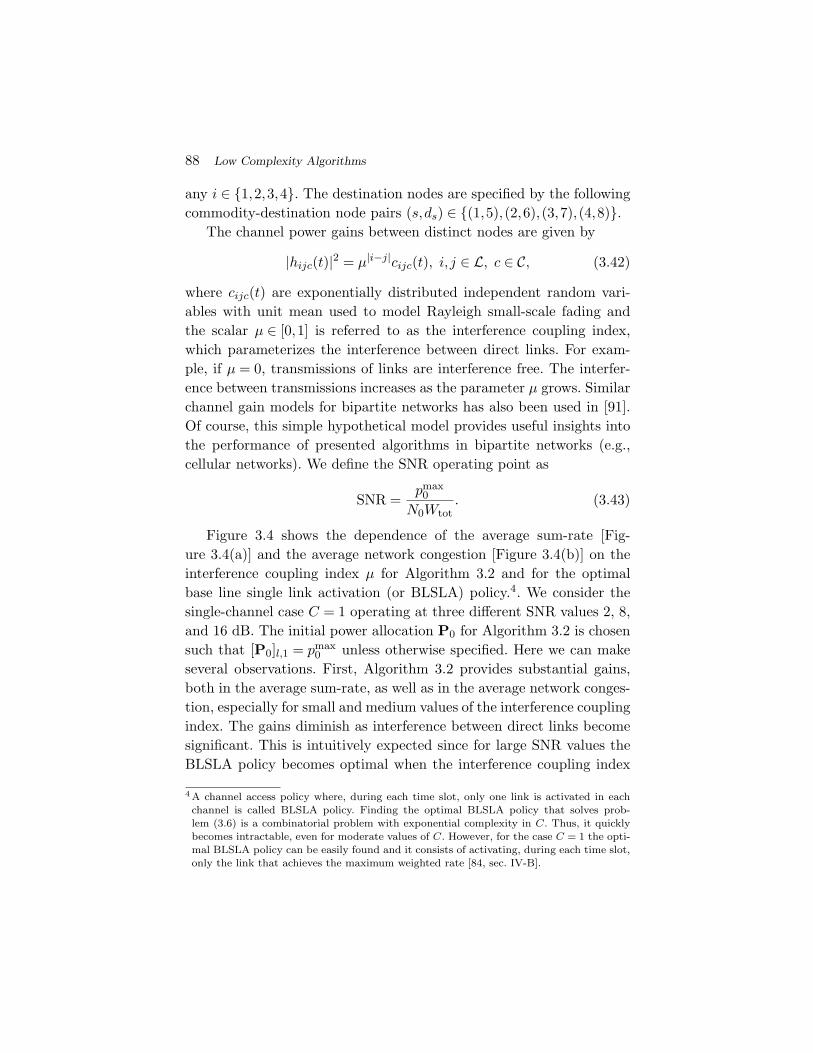
88 Low Complexity Algorithms
any i ∈ {1,2,3,4}. The destination nodes are specified by the followingcommodity-destination node pairs (s,ds) ∈ {(1,5),(2,6),(3,7),(4,8)}.
The channel power gains between distinct nodes are given by
|hijc(t)|2 = µ|i−j|cijc(t), i, j ∈ L, c ∈ C, (3.42)
where cijc(t) are exponentially distributed independent random vari-ables with unit mean used to model Rayleigh small-scale fading andthe scalar µ ∈ [0,1] is referred to as the interference coupling index,which parameterizes the interference between direct links. For exam-ple, if µ = 0, transmissions of links are interference free. The interfer-ence between transmissions increases as the parameter µ grows. Similarchannel gain models for bipartite networks has also been used in [91].Of course, this simple hypothetical model provides useful insights intothe performance of presented algorithms in bipartite networks (e.g.,cellular networks). We define the SNR operating point as
SNR =pmax0
N0Wtot. (3.43)
Figure 3.4 shows the dependence of the average sum-rate [Fig-ure 3.4(a)] and the average network congestion [Figure 3.4(b)] on theinterference coupling index µ for Algorithm 3.2 and for the optimalbase line single link activation (or BLSLA) policy.4. We consider thesingle-channel case C = 1 operating at three different SNR values 2, 8,and 16 dB. The initial power allocation P0 for Algorithm 3.2 is chosensuch that [P0]l,1 = pmax
0 unless otherwise specified. Here we can makeseveral observations. First, Algorithm 3.2 provides substantial gains,both in the average sum-rate, as well as in the average network conges-tion, especially for small and medium values of the interference couplingindex. The gains diminish as interference between direct links becomesignificant. This is intuitively expected since for large SNR values theBLSLA policy becomes optimal when the interference coupling index
4 A channel access policy where, during each time slot, only one link is activated in eachchannel is called BLSLA policy. Finding the optimal BLSLA policy that solves prob-lem (3.6) is a combinatorial problem with exponential complexity in C. Thus, it quicklybecomes intractable, even for moderate values of C. However, for the case C = 1 the opti-mal BLSLA policy can be easily found and it consists of activating, during each time slot,only the link that achieves the maximum weighted rate [84, sec. IV-B].
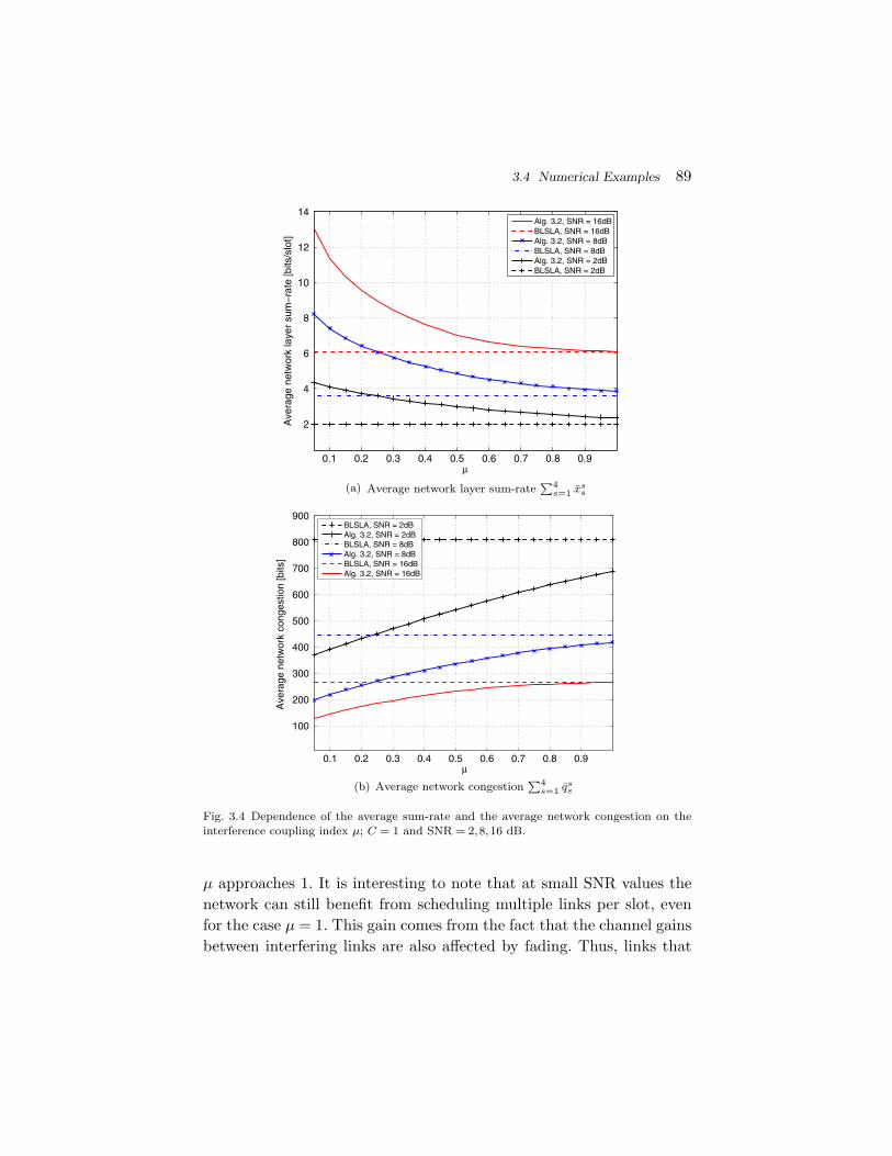
3.4 Numerical Examples 89
0.1 0.2 0.3 0.4 0.5 0.6 0.7 0.8 0.9
2
4
6
8
10
12
14
µ
Ave
rage
net
wor
k la
yer
sum
−ra
te [b
its/s
lot]
Alg. 3.2, SNR = 16dBBLSLA, SNR = 16dBAlg. 3.2, SNR = 8dBBLSLA, SNR = 8dBAlg. 3.2, SNR = 2dBBLSLA, SNR = 2dB
0.1 0.2 0.3 0.4 0.5 0.6 0.7 0.8 0.9
100
200
300
400
500
600
700
800
900
µ
Ave
rage
net
wor
k co
nges
tion
[bits
]
BLSLA, SNR = 2dBAlg. 3.2, SNR = 2dBBLSLA, SNR = 8dBAlg. 3.2, SNR = 8dBBLSLA, SNR = 16dBAlg. 3.2, SNR = 16dB
Fig. 3.4 Dependence of the average sum-rate and the average network congestion on theinterference coupling index µ; C = 1 and SNR = 2,8,16 dB.
µ approaches 1. It is interesting to note that at small SNR values thenetwork can still benefit from scheduling multiple links per slot, evenfor the case µ = 1. This gain comes from the fact that the channel gainsbetween interfering links are also affected by fading. Thus, links that

90 Low Complexity Algorithms
experience low instantaneous interference levels can be simultaneouslyscheduled. Results suggest that, especially for small and medium val-ues of the interference coupling index, the given method often yieldsdesigns that are far superior to those obtained by BLSLA.
Figure 3.5 shows the dependence of the average sum-rate[Figure 3.5(a)] and of the average network congestion [Figure 3.5(b)]on the number of iterations of Algorithm 3.2. We consider the single-channel case C = 1 with interference coupling index µ = 0.5 and SNRvalues 2, 8, and 16 dB. To facilitate faster convergence, Algorithm 3.2is run without considering the trust region constraints; to do this, wecan simply set the parameter α in Algorithm 3.2 to a very large positivenumber, e.g., α = 10100 [see problem (3.18)]. As a reference, we considerthe optimal BLSLA policy. Results show that the incremental benefitsare very significant for the first few iterations and are marginal later.For example, in the case of SNR = 16 dB, when the numbers of iter-ations changes from 1 to 3, the improvement in the average sum-rateis around 18.1%, whereas when it changes from 7 to 9, the improve-ment is around 0.30%. Therefore, by running Algorithm 3.2 for a fewiterations (e.g., 5 iterations) we can yield performance levels that arealmost indistinguishable from those that would have been obtained byrunning Algorithm 3.2 until it terminates (see the stopping criterion instep 3). This observation can be very useful in practice, since we canterminate Algorithm 3.2 when the incremental improvements betweenconsecutive iterations become negligible.
Figure 3.6 shows the dependence of the average sum-rate[Figure 3.6(a)] and of the average network congestion [Figure 3.6(b)]on the SNR for Algorithm 3.2 and optimal BLSLA policy. We haveconsidered the case C = 1 and µ = 0.3. For comparison, we also plotthe results due to a commonly used high SINR approximation [29]where the achievable rates log(1 + γlc) are approximated by log(γlc).In particular, the objective function of problem (3.11) is approximatedby
∏c∈C
∏l∈L γ−βl
lc . Recall that γlc represents the SINR of link l inchannel c and βl represents the differential backlog of link l. Thisresults in a convex approximation (i.e., a GP) of problem (3.11).One should not confuse high SINR with high SNR, since those arefundamentally different and a high SNR value does not ensure high

3.4 Numerical Examples 91
1 2 3 4 5 6 7 8 9 10
2
3
4
5
6
7
8
9
Iteration
Ave
rage
net
wor
k la
yer
sum
−ra
te [b
its/s
lot]
Alg. 3.2, SNR = 16dBBLSLA, SNR = 16dBAlg. 3.2, SNR = 8dBBLSLA, SNR = 8dBAlg. 3.2, SNR = 2dBBLSLA, SNR = 2dB
1 2 3 4 5 6 7 8 9 10200
300
400
500
600
700
800
900
Iteration
Ave
rage
net
wor
k co
nges
tion
[bits
]
BLSLA, SNR = 2dBAlg. 3.2, SNR = 2dBBLSLA, SNR = 8dBAlg. 3.2, SNR = 8dBBLSLA, SNR = 16dBAlg. 3.2, SNR = 16dB
Fig. 3.5 Dependence of the average sum-rate and the average network congestion on theiteration; µ = 0.5, C = 1, and SNR = 2,8,16 dB.
SINR values in all links. Results show that, when compared with othermethods, RA based on Algorithm 3.2 offers larger average sum-rateas well as reduced average network congestion. The relative gainsof Algorithm 3.2 reduce, compared to the BLSLA at high SNR, forexample, the relative gain offered by Algorithm 3.2 in the average
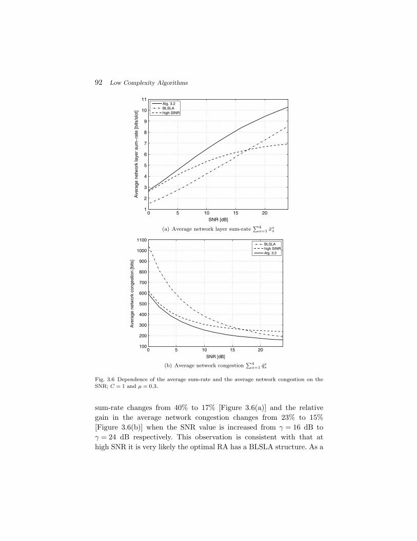
92 Low Complexity Algorithms
0 5 10 15 201
2
3
4
5
6
7
8
9
10
11
SNR [dB]
Ave
rage
net
wor
k la
yer
sum
−ra
te [b
its/s
lot]
Alg. 3.2BLSLAhigh SINR
0 5 10 15 20100
200
300
400
500
600
700
800
900
1000
1100
SNR [dB]
Ave
rage
net
wor
k co
nges
tion
[bits
]
BLSLAhigh SINRAlg. 3.2
Fig. 3.6 Dependence of the average sum-rate and the average network congestion on theSNR; C = 1 and µ = 0.3.
sum-rate changes from 40% to 17% [Figure 3.6(a)] and the relativegain in the average network congestion changes from 23% to 15%[Figure 3.6(b)] when the SNR value is increased from γ = 16 dB toγ = 24 dB respectively. This observation is consistent with that athigh SNR it is very likely the optimal RA has a BLSLA structure. As a

3.4 Numerical Examples 93
result, at the optimal RA, different links correspond to different SINRregions, and therefore the high SINR approximation is, of course,unreasonable and suffers a large penalty, especially at high SNR values.This poor performance is qualitatively consistent with intuition: thesolution obtained by employing high SINR approximation in RA mustcontain all nonzero entries (i.e., nonzero γlc) to drive the approximatedobjective
(i.e.,
∏c∈C
∏l∈L γ−βl
lc
)into a nonzero value, and therefore
never yields a solution to the form of BLSLA.Figure 3.7 shows the dependence of the average sum-rate [Fig-
ure 3.7(a)] and of the average network congestion [Figure 3.7(b)] onthe number of channels C for Algorithm 3.2. We consider the caseSNR = 16 dB and µ = 0.3 and the initial power allocation P0 forAlgorithm 3.2 is simply chosen such that [P0]l,c = pmax
0 /C. The plotsillustrate that increasing the number of channels will yield betterperformance in both the average sum-rate and the average networkcongestion (e.g., when the number of channels C changes from 1 to 8,the improvement in the average sum-rate and the reduction in averagenetwork congestion is around 12% and 12.4%, respectively). We stressthat the benefits are solely achieved by opportunistically exploitingthe available multichannel diversity in the network via Algorithm 3.2without any supplementary bandwidth or power consumption. More-over, the incremental benefits are very significant for small C, forexample, when the number of channels C changes from 1 to 2, theimprovement in the average sum-rate is around 6%, whereas whenC changes from 7 to 8, the improvement is around 0.25%. The plotsgive much insight into why multichannel designs are important andbeneficial compared to the single-channel counterpart.
3.4.2 NUM for Nonbipartite Networks with SingleuserDetection at Receivers
First, two small fully connected multihop wireless network setups,which are identical to the once shown in Figure 2.11 are considered.
We assume an exponential path loss model; the channel power gains|hijc(t)|2 between distinct nodes are given by
|hijc(t)|2 =(
dij
d0
)−η
cijc(t), (3.44)
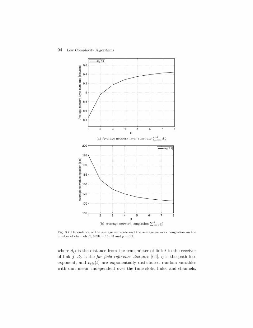
94 Low Complexity Algorithms
1 2 3 4 5 6 7 8
8.4
8.6
8.8
9
9.2
9.4
9.6
C
Ave
rage
net
wor
k la
yer
sum
−ra
te [b
its/s
lot]
Alg. 3.2
1 2 3 4 5 6 7 8165
170
175
180
185
190
195
200
C
Ave
rage
net
wor
k co
nges
tion
[bits
]
Alg. 3.2
Fig. 3.7 Dependence of the average sum-rate and the average network congestion on thenumber of channels C; SNR = 16 dB and µ = 0.3.
where dij is the distance from the transmitter of link i to the receiverof link j, d0 is the far field reference distance [64], η is the path lossexponent, and cijc(t) are exponentially distributed random variableswith unit mean, independent over the time slots, links, and channels.

3.4 Numerical Examples 95
The first term of (3.44) represents the path loss factor and the secondterm models Rayleigh small-scale fading. The SNR operating point isdefined as
SNR =pmax0
N0Wtot
(D0
d0
)−η
. (3.45)
In the following simulations we set D0/d0 = 10 and η = 4.Figure 3.8 shows the dependence of the average network layer sum-
rate on the SNR for the considered network setups, where we use C = 1.As a benchmark, we first consider the branch and bound algorithm pre-sented in Section 2.2 to optimally solve the RA subproblem. It shouldbe stressed that the optimality of the algorithm given in Section 2.2is achieved at the expense of prohibitive computational complexity,even in the case of very small problem instances. We then considerthe optimal BLSLA policy and Algorithm 3.3 with two initializationmethods: (1) Uniform initialization and (2) BLSLA based initializa-tion. In the case of uniform initialization the initial power allocationP0 is chosen such that [P0]l,1 = pmax
0 /(|Otran(l)|). In the case of BLSLAbased initialization the initial power allocation P0 is chosen such that[P0]l�,1 : [P0]j,1 = P : 1 for all j ∈ L, j �= l� where l� is the index of theactive link obtained based on the optimal BLSLA policy and P � 1 is areal number. For comparison, we also plot the results for Algorithm 3.2with uniform and BLSLA initializations.
Results show that the performance of Algorithm 3.3 is very close tothe optimal branch and bound algorithm. Specifically, Algorithm 3.3with BLSLA initialization is almost indistinguishable from the opti-mum and at least as good as the optimal BLSLA, for all consideredcases. In contrast, Algorithm 3.3 with uniform initialization exhibitssignificant deviations from both the optimal branch and bound algo-rithm and BLSLA, specially at high SNR values. This behavior is notsurprising since Algorithm 3.3 is a local method for the nonconvexproblem (3.6). Therefore, the initialization point of the algorithm caninfluence the resulting solution [22, sec. 1.4.1]. Nevertheless, a care-fully selected initialization point can improve the performance of Algo-rithm 3.3 to very close to the optimum. For example, at high SNRvalues, the performance of Algorithm 3.3 with BLSLA initialization is

96 Low Complexity Algorithms
0 2 4 6 8 10 12 14 160
0.5
1
1.5
2
2.5
3
3.5
SNR [dB]
Ave
rage
net
wor
k la
yer
sum
−ra
te [b
its/s
lot]
Alg. 2.1 (section 2.2)Alg. 3.3, BLSLA init.Alg. 3.3, uniform init.BLSLAAlg. 3.2, BLSLA init.Alg. 3.2, uniform init.
0 2 4 6 8 10 12 14 160
0.5
1
1.5
2
2.5
3
SNR [dB]
Ave
rage
NW
laye
r su
m−
rate
[bits
/slo
t]
Alg. 2.1 (section 2.2)Alg. 3.3, BLSLA init.Alg. 3.3, uniform init.BLSLAAlg. 3.2, BLSLA init.Alg. 3.2, uniform init.
Fig. 3.8 (a) Dependence of the average network layer sum-rate on SNR for network 1[Figure 2.11(a)]; (b) Dependence of the average network layer sum-rate on SNR for network 2[Figure 2.11(b)].
almost identical to the optimum, whereas the performance with uni-form initialization deviates a bit from the optimum. It is important toremark that at low and moderate values of SNR, results derived fromAlgorithm 3.3 are not significantly affected by the initialization method.

3.4 Numerical Examples 97
Results also show that, in the presence of self interferers, Algorithm 3.2cannot perform well and it can converge to a very bad suboptimal point,as we pointed out in Section 3.2.4. Therefore, even though the com-putational complexity of Algorithm 3.3 does not increase more thanpolynomially with the problem size, results show that Algorithm 3.3with a proper initialization performs close to the optimum.
Next, a larger network; a fully connected multihop, multicommoditywireless network as shown in Figure 3.9 is considered. There are N = 9nodes and S = 3 commodities. The commodities arrive exogenouslyat different nodes in the network as described in Table 3.1. Thus wehave S1 = {2},S2 = {3},S3 = {3},S5 = {2},S7 = {1,3}, and Si = ∅ forall i ∈ {4,6,8,9}. The nodes are located in a rectangular grid such thatthe horizontal and vertical distances between adjacent nodes are D0 m.The channel power gains, between nodes, are given by (3.44) and theSNR operating point is given by (3.45). Moreover, we set D0/d0 = 10and η = 4.
Figure 3.10 shows the dependence of the average sum-rate[Figure 3.10(a)] and of the average network congestion [Figure 3.10(b)]
Fig. 3.9 Multihop wireless network with N = 9 nodes and S = 3 commodities.
Table 3.1. Network commodities, destination nodes, andsource nodes.
Commodity (s) Destination node (ds) Source nodes
1 2 72 3 1,53 9 2,3,7

98 Low Complexity Algorithms
0 5 10 15 20 25 30 35 400
1
2
3
4
5
6
7
8
9
10
11
SNR [dB]
Ave
rage
net
wor
k la
yer
sum
−ra
te [b
its/s
lot]
Alg. 3.3, BLSLA init.Alg. 3.3, uniform init.BLSLAAlg. 3.2, greedy partitioningAlg. 3.2, random partitioninghigh SINR, greedy partitioninghigh SINR, random partitioning
0 5 10 15 20 25 30 35 40
0.2
0.4
0.6
0.8
1
1.2
1.4
1.6
1.8
2x 10
4
SNR [dB]
Ave
rage
net
wor
k co
nges
tion
[bits
]
high SINR, random partitioninghigh SINR, greedy partitioningAlg. 3.2, random partitioningAlg. 3.2, greedy partitioningBLSLAAlg. 3.3, uniform init.Alg. 3.3, BLSLA init.
Fig. 3.10 Dependence of the average sum-rate and the average network congestion on theSNR; C = 1.
on the SNR for several algorithms, where we use C = 1. First we haveconsidered the optimal BLSLA policy and Algorithm 3.3 with the twoinitialization methods: (1) Uniform initialization and (2) BLSLA basedinitialization (the same initializations as used when plotting Figure 3.8).

3.4 Numerical Examples 99
For comparison, we also plot the results for the low-complex approacheswhere the set of nodes N is first partitioned into two disjoint subsets,the set of transmitting nodes T and the set of receiving nodes R andthen Algorithm 3.2 and high SINR approximation are used in RA. Thepartitioning of the set of nodes N into two disjoint subsets is performedusing two simple methods: (1) random partitioning and (2) greedy par-titioning based on differential backlogs. In random partitioning, eachnode is allocated either to T or to R with equal probabilities. Greedypartitioning is performed as follows. We start with an empty set of linksL = ∅. At each step, the link l� from the set L \ L which has the largestdifferential backlog βl (i.e., l� = argmaxl∈L\L βl) is added to the set L.Then all links outgoing from rec(l�) and all links incoming to tran(l�)are deleted from L. This procedure continues until there are no linksleft in L \ L. The sets T and R can be found as T = {tran(l)|l ∈ L}and R = {rec(l)|l ∈ L}.
From Figure 3.10 we make the following observations. First, Algo-rithm 3.3 with BLSLA based initialization yields results better than anyother counterpart. In contrast, Algorithm 3.3 with uniform initializa-tion shows significant deviations from the BLSLA solution at high SNR,especially in the terms of average sum-rate [Figure 3.10(a)]. Moreover,it is important to observe again that at low and moderate values ofSNR, results derived from Algorithm 3.3 are not substantially affectedby the initialization method. These observations are almost the sameas those we saw in Figure 3.8. We also observe that Algorithm 3.3 witha proper initialization, can significantly outperform Algorithm 3.2 inconjunction with either random or greedy partitioning. This elaboratesthe importance of gradual self-interference gain increments (i.e., step 4of Algorithm 3.3) in finding a better RA compared to the direct appli-cation of Algorithm 3.2 with heuristic partitioning. In most cases thereis no advantage to using high SINR approximation. These observa-tions are very useful in practice since they illustrate that Algorithm 3.3often works well when initialized with a reasonable starting point (e.g.,BLSLA based initialization). In addition, we note that even with a verysimple initialization, for example, uniform initialization, Algorithm 3.3yields substantial gains, especially at small and moderate SNR values(e.g., 0 dB–20 dB).

100 Low Complexity Algorithms
1 2 3 4 5 6 7 83
3.5
4
4.5
5
5.5
6
6.5
C
Ave
rage
net
wor
k la
yer
sum
−ra
te [b
its/s
lot]
Alg. 3.3, uniform init.Alg. 3.2, greedy partitioningAlg. 3.2, random partitioning
1 2 3 4 5 6 7 8
1800
2000
2200
2400
2600
2800
3000
C
Ave
rage
net
wor
k co
nges
tion
[bits
]
Alg. 3.2, random partitioningAlg. 3.2, greedy partitioningAlg. 3.3, uniform init.
Fig. 3.11 Dependence of the average sum-rate and the average network congestion on thenumber of channels C; SNR = 16 dB.
Figure 3.11 shows the dependence of the average sum-rate[Figure 3.11(a)] and of the average network congestion [Figure 3.11(b)]on the numbers of channels C for Algorithm 3.3. We have consideredthe case SNR = 16 dB and have considered a uniform initialization for

3.4 Numerical Examples 101
Algorithm 3.3 where the initial power allocation P0 is chosen such that[P0]l,c = pmax
0 /(C.|Otran(l)|). For comparison, we also plot the resultsfor Algorithm 3.2 with random and greedy partitioning of nodes N .The results are consistent with the previous observations in Figure 3.7,that is, as the number of channels increases better performance in boththe average sum-rate and the average network congestion is achieved.These benefits are again obtained by opportunistically exploiting theavailable multichannel diversity in the network via the algorithms pre-sented. Moreover, the results suggest that using Algorithm 3.3 in theRA can increase the gains very significantly, compared to the RA basedon simple extensions to Algorithm 3.2, which runs with either randomor greedy partitioning of nodes. For example, the relative gains in theaverage sum-rate are above 23% [Figure 3.11(a)] and the relative gainsin the average network congestion are above 4.7% [Figure 3.11(b)] overthe range of interest, C = 1 to C = 8.
3.4.3 Effect of Self Interference Cancelation
For the considered network setups in this section, the channel powergains between nodes are given by (3.44) and the SNR operating point isgiven by (3.45). For illustration purposes we consider a single-channelcase (i.e., C = 1). Moreover, we set D0/d0 =
√10 and η = 4. In all the
simulations in this subsection, Algorithm 3.3 with BLSLA based ini-tialization is considered.
Inspired by the Gaussian two-way channel [36], we first consider asimple two node wireless network as shown in Figure 3.12(a). There aretwo commodities, the first one arrives at node 1, and is intended fornode 2; the second commodity arrives at node 2, and is intended for
(a) (b)
Fig. 3.12 (a) Two node wireless network with N = 2 nodes, L = 2 links, and S = 2 com-modities. Different commodities are represented by different color; (b) Tandem wirelessnetwork with N = 4 nodes and S = 2 commodities. Different commodities are representedby different color.
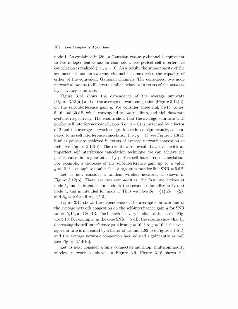
102 Low Complexity Algorithms
node 1. As explained in [36], a Gaussian two-way channel is equivalentto two independent Gaussian channels where perfect self interferencecancelation is realized (i.e., g = 0). As a result, the sum-capacity of thesymmetric Gaussian two-way channel becomes twice the capacity ofeither of the equivalent Gaussian channels. The considered two nodenetwork allows us to illustrate similar behavior in terms of the networklayer average sum-rate.
Figure 3.13 shows the dependence of the average sum-rate[Figure 3.13(a)] and of the average network congestion [Figure 3.13(b)]on the self-interference gain g. We consider three link SNR values,5,16, and 30 dB, which correspond to low, medium, and high data ratesystems respectively. The results show that the average sum-rate withperfect self interference cancelation (i.e., g = 0) is increased by a factorof 2 and the average network congestion reduced significantly, as com-pared to no self interference cancelation (i.e., g = 1); see Figure 3.13(a).Similar gains are achieved in terms of average network congestion aswell; see Figure 3.13(b). The results also reveal that, even with animperfect self interference cancelation technique, we can achieve theperformance limits guaranteed by perfect self interference cancelation.For example, a decrease of the self-interference gain up to a valueg = 10−4 is enough to double the average sum-rate for link SNR = 5 dB.
Let us now consider a tandem wireless network, as shown inFigure 3.12(b). There are two commodities, the first one arrives atnode 1, and is intended for node 4; the second commodity arrives atnode 4, and is intended for node 1. Thus we have S1 = {1},S4 = {2},and Sn = ∅ for all n ∈ {2,3}.
Figure 3.14 shows the dependence of the average sum-rate and ofthe average network congestion on the self-interference gain g for SNRvalues 5,16, and 30 dB. The behavior is very similar to the case of Fig-ure 3.13. For example, in the case SNR = 5 dB, the results show that bydecreasing the self-interference gain from g = 10−1 to g = 10−4 the aver-age sum-rate is increased by a factor of around 1.82 [see Figure 3.14(a)]and the average network congestion has reduced significantly as well[see Figure 3.14(b)].
Let us next consider a fully connected multihop, multicommoditywireless network as shown in Figure 3.9. Figure 3.15 shows the

3.4 Numerical Examples 103
0
2
4
6
8
10
12
14
16
18
20
Ave
rage
net
wor
k la
yer
sum
−ra
te [b
its/s
lot]
Alg. 3.3, SNR = 30dBBLSLA, SNR = 30dBAlg. 3.3, SNR = 16dBBLSLA, SNR = 16dBAlg. 3.3, SNR = 5dBBLSLA, SNR = 5dB
10−10 10−8 10−6 10−4 10−2 1000
500
1000
1500
2000
2500
g
10−10 10−8 10−6 10−4 10−2 100
g
Ave
rage
net
wor
k co
nges
tion
[bits
]
BLSLA, SNR = 5dBAlg. 3.3, SNR = 5dBBLSLA, SNR = 16dBAlg. 3.3, SNR = 16dBBLSLA, SNR = 30dBAlg. 3.3, SNR = 30dB
Fig. 3.13 Dependence of the average sum-rate and of the average network congestion onthe self-interference gain g in the case of the two node wireless network.
dependence of the average sum-rate and of the average network con-gestion on the self-interference gain g for SNR values 5,16, and 30 dB.Let us first consider the case of a low SNR value, i.e., SNR = 5 dB. Theresults show that by decreasing the self-interference gain from g = 10−1
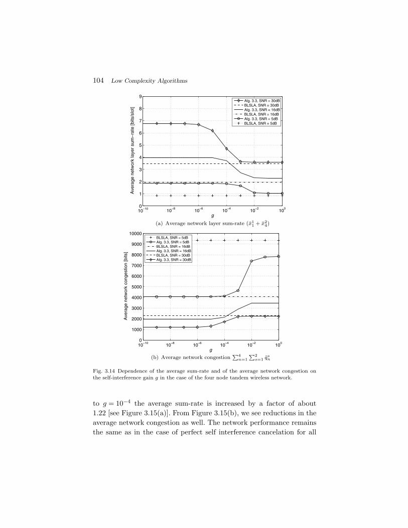
104 Low Complexity Algorithms
0
1
2
3
4
5
6
7
8
9
Ave
rage
net
wor
k la
yer
sum
−ra
te [b
its/s
lot]
Alg. 3.3, SNR = 30dBBLSLA, SNR = 30dBAlg. 3.3, SNR = 16dBBLSLA, SNR = 16dBAlg. 3.3, SNR = 5dBBLSLA, SNR = 5dB
10−10
10−8
10−6
10−4
10−2
100
0
1000
2000
3000
4000
5000
6000
7000
8000
9000
10000
g
Ave
rage
net
wor
k co
nges
tion
[bits
]
BLSLA, SNR = 5dBAlg. 3.3, SNR = 5dBBLSLA, SNR = 16dBAlg. 3.3, SNR = 16dBBLSLA, SNR = 30dBAlg. 3.3, SNR = 30dB
10−10 10
−810
−610
−410
−210
0
g
Fig. 3.14 Dependence of the average sum-rate and of the average network congestion onthe self-interference gain g in the case of the four node tandem wireless network.
to g = 10−4 the average sum-rate is increased by a factor of about1.22 [see Figure 3.15(a)]. From Figure 3.15(b), we see reductions in theaverage network congestion as well. The network performance remainsthe same as in the case of perfect self interference cancelation for all

3.4 Numerical Examples 105
10−10 10−8 10−6 10−4 10−2 100
2
3
4
5
6
7
8
9
10
11
g
Ave
rage
net
wor
k la
yer
sum
−ra
te [b
its/s
lot]
Alg. 3.3, SNR = 30dBBLSLA, SNR = 30dBAlg. 3.3, SNR = 16dBBLSLA, SNR = 16dBAlg. 3.3, SNR = 5dBBLSLA, SNR = 5dB
1000
1500
2000
2500
3000
3500
4000
4500
5000
5500
6000
6500
Ave
rage
net
wor
k co
nges
tion
[bits
]
BLSLA, SNR = 5dBAlg. 3.3, SNR = 5dBBLSLA, SNR = 16dBAlg. 3.3, SNR = 16dBBLSLA, SNR = 30dBAlg. 3.3, SNR = 30dB
10−10 10−8 10−6 10−4 10−2 100
g
Fig. 3.15 Dependence of the average sum-rate and of the average network congestion onthe self-interference gain g in the case of the nine node multihop wireless network.
values of g < 10−4. In this region the network performance is limitedby the interference between distinct nodes, and no further improve-ment is possible by only increasing the accuracy of the self interferencecancelation. On the other hand, no gain in the network performance is
106 Low Complexity Algorithms
achieved by using an imperfect self interference cancelation techniquewhich leads to g > 10−1. In this region the RA solution provided byAlgorithm 3.3 is always admissible (i.e., no node transmits and receivessimultaneously).
In each considered network setup (i.e., Figures 3.12(a), 3.12(b),and 3.9) a similar behavior of the results holds for medium and highSNR values as well (i.e., SNR = 16 and 30 dB). Moreover, as we changeSNR from low values to high values, the accuracy level required bythe self interference cancelation becomes more stringent. For example,in the case of the fully connected multihop, multicommodity wirelessnetwork in figure 3.9, if the SNR operating point is changed from5 to 30 dB, then the accuracy level required by the self interferencecancelation should be improved from g = 10−1 to g = 10−3 to startgaining in network layer performances. This is intuitively expectedsince, the larger the SNR operating point, the larger the power levelsof the nodes, and therefore the higher the accuracy level required bythe self interference cancelation techniques to remove the increasedtransmit power at nodes.
Note that the relative gains due to self interference cancelationin the considered fully connected multihop network [Figure 3.9] aresmaller compared to the relative gains experienced in the tandem wire-less network [Figure 3.12(b)]. This behavior is intuitively explainedby looking in to the network topology. When the self interference issignificantly canceled, the resultant interference at the receiver nodeof any link in the case of the tandem multihop wireless network inFigure 3.12(b) is smaller on average to that of the multihop wirelessnetwork in Figure 3.9; note that any receiver node of the fully con-nected multihop network has many adjacent interfering nodes. Thus,with zero self interference, links in the tandem network can operate atlarger rates, and therefore yields larger relative gains.
Finally, we show by an example, how to apply rate-equivalence (3.28) to find the required value of self-interferencegain g in order to preserve network layer performances if the distancebetween nodes is scaled. Let us construct a new network by scaling thedistances between the nodes of the original network (see Figure 3.9) by

3.4 Numerical Examples 107
a factor of θ =√
10 and the maximum node transmission power pmax0
by a factor of θη = 100 (note that η = 4). We refer to this new networkas the scaled network. To illustrate the idea let us consider the caseSNR = 5 dB in Figure 3.10 and focus to the point g = 10−4 for whichthe average sum-rate is 3.5 [bits/slot]. The value of g at this point canbe considered as the minimum required accuracy level of self inter-ference cancelation to achieve an average sum-rate of 3.5 bits/slot inthe original network. Now we ask what is the required self-interferencegain gnew that would result in the same average sum-rate value (i.e.,3.5 bits/slot) in the scaled network. From (3.28) it follows that therequired accuracy level of self interference cancelation should beimproved at least to a level of gnew = g/θη = 10−4/100 = 10−6.
3.4.4 NUM for Networks with Multiuser Detection atReceivers
The network in Figure 3.9 is considered. The assumptions and thesimulation parameters are exactly the same as in Section 3.4.2.
Figure 3.16 shows the dependence of the average sum-rate[Figure 3.16(a)] and of the average network congestion [Figure 3.16(b)]on the SNR for RA where only one node is allowed to transmit in eachslot and receivers perform multiuser detection. For illustration pur-poses we consider the single-channel case (i.e., C = 1). We also showthe results for a nonfading case [i.e., by having cijc(t) = 1 in (3.24)]for comparison. Here we can make several observations. Fading cansignificantly improve the overall performance in average sum-rate andaverage network congestion. This observation has an analogy with mul-tiuser diversity in downlink fading channels [124, sec. 6.6]. Intuitionsuggests that when there are many links which fade independently, atany time slot there is a high probability that the resulting rate andpower allocation yields a better schedule (see [43, sec. 4.7]) comparedto the nonfading case. There are significant advantages to having mul-tiuser detection, especially for high SNR values. At low SNR, gains aremarginal. Thus, multiuser detectors have a practical advantage oversingleuser detectors, especially in a high SINR regime. For example,
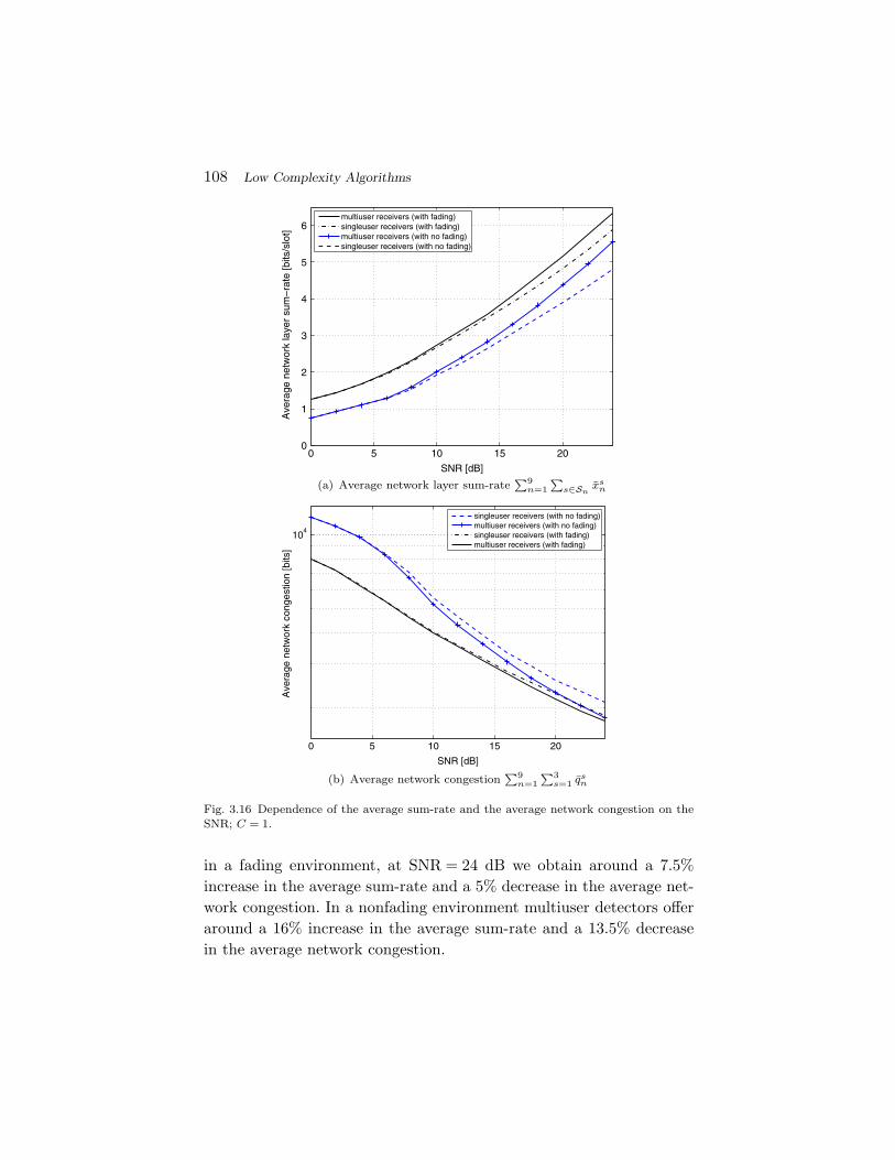
108 Low Complexity Algorithms
0 5 10 15 200
1
2
3
4
5
6
SNR [dB]
Ave
rage
net
wor
k la
yer
sum
−ra
te [b
its/s
lot]
multiuser receivers (with fading)singleuser receivers (with fading)multiuser receivers (with no fading)singleuser receivers (with no fading)
0 5 10 15 20
104
SNR [dB]
Ave
rage
net
wor
k co
nges
tion
[bits
]
singleuser receivers (with no fading)multiuser receivers (with no fading)singleuser receivers (with fading)multiuser receivers (with fading)
Fig. 3.16 Dependence of the average sum-rate and the average network congestion on theSNR; C = 1.
in a fading environment, at SNR = 24 dB we obtain around a 7.5%increase in the average sum-rate and a 5% decrease in the average net-work congestion. In a nonfading environment multiuser detectors offeraround a 16% increase in the average sum-rate and a 13.5% decreasein the average network congestion.

3.5 Summary and Discussion 109
3.5 Summary and Discussion
We considered the power and rate control problem in a wireless net-work in conjunction with the next-hop routing/scheduling and the flowcontrol problem. Thus, although the focus lies on the so-called resourceallocation problem that is confined to the physical/medium access con-trol layers, its formulation captures interactions with the higher-layersin a manner similar to the one employed in [82]. The result is a crosslayer formulation. The problem, unfortunately, is NP-hard, and there-fore there are no polynomial time algorithms to solve it. Our presen-tation has been to consider first a general access operation, but witha relatively simple form of receiver structure (bank of match filters),and then to limit the access operation to a single node at a time (eithertransmitting or receiving) but allowing for increased multiuser detectorcomplexity at the receiver.
In the first case, we presented a new optimization methodologybased on homotopy methods and complementary geometric program-ming solution methods. Numerical results showed that the presentedalgorithms perform close to exponentially complex optimal solutionmethods. In addition, they are in fact fast and are capable of handlinglarge-scale problems.
The considered method was also used to evaluate the gains achiev-able at the network layer when the network nodes employ selfinterference cancelation techniques with different degrees of accuracy.Numerical results showed that the self interference cancelation requiresa certain level of accuracy to obtain quantifiable gains at the networklayer. The gains saturate after a certain cancelation accuracy. The levelof accuracy required by the self interference cancelation techniquesdepends on many factors, such as the distances between the networknodes and the operating power levels of the network nodes. For theconsidered network setups, the numerical results showed that a selfinterference reduction in the range 20−60 dB leads to significant gainsat the network layer. We emphasize that this level of accuracy is prac-tically achievable, for example, the recent proposals [32, 100, 101, 102]provide cost effective mechanisms for an up to 55 dB reduction in theself-interference coefficient. These observations are indeed important in
110 Low Complexity Algorithms
the context of certain future cellular systems. For example, as the trendin cellular systems is to increase the data rates of users by introducingvery small cells (e.g., femtocells), the difference between transmittedand received power might not be very large. Therefore, self interfer-ence cancelation strategies can be of great benefit to such systems.Numerical results further showed that the topology of the network hasa substantial influence on performance gains. For example, in the caseof tandem multihop wireless networks, the benefits due to self inter-ference cancelation are more pronounced when compared to those of amultihop network, in which the nodes are located in a square grid.
In the second case, we obtained a complete solution and illustratenumerically the performance gain due to multiuser detector capability.The main benefit here is the simplicity of the solution methods. As aresult, these simple access protocols can be potentially useful in prac-tical applications with more advanced communication systems.

4A Distributed Approach
This section present a distributed method for WSRMax problem ina multicell MISO downlink system. Unlike the WMMSE algorithm1
proposed in [110], the method presented in this section does not relyon user terminals’ assistance such as estimations, computations, andfeedback information to base stations over the air interface. Only basestation to base station (BS) synchronized communication is required,where all the signalling overhead is exchanged through reliable back-haul links (e.g., fiber and microwave links). All the necessary com-putation can be carried out asynchronously at each BS without anyinvolvement of the user terminals. Thus, the algorithm presented inthis section is well suited for systems where the user terminal sup-port is not allowed or not desirable. The algorithm is based on primaldecomposition methods and subgradient methods [17, 19]. Specifically,primal decomposition techniques [17] are applied to split the probleminto a master problem and many subproblems. In the case of masterproblem, a sequential convex approximation strategy [18] together witha subgradient method [19] that relies on BS coordinations is adopted.
1 We use the same acronym WMMSE to refer to this algorithm as suggested in [110].
111
112 A Distributed Approach
In the case of subproblems, an existing algorithm originally proposedin [34, sec. 4.3], which is based on second-order cone programming(SOCP) [73] and geometric programming (or GP) [20] is adopted. Thesubproblems (or BS optimizations) can be carried out in a fully asyn-chronous manner. With appropriate choice of stopping criteria, themonotonic convergence of the algorithm is guaranteed. Practical stop-ping criteria, which are favorable for implementing the algorithm, butat the expense of a sacrificing the monotone convergence are also pre-sented. Numerical results are provided to compare this method withWMMSE algorithm [110], the GP/SOCP based algorithm proposedin [34, sec. 4.3], and the distributed algorithm proposed in [10, 11].The behavior of the algorithm under different degrees of BS coordina-tion is also discussed and numerically illustrated.
4.1 System Model and Problem Formulation
A multicell MISO downlink system, with N BSs each equipped with T
transmit antennas is considered. The set of all BSs is denoted by N andwe label them with the integer values n = 1, . . . ,N . The transmissionregion of each BS is modeled as a disc with radius RBS centered atthe location of the BS. Single data stream is transmitted for each user.We denote the set of all data streams in the system by L and labelthem with the integer values l = 1, . . . ,L. The transmitter node (i.e.,the BS) of lth data stream is denoted by tran(l) and the receiver nodeof lth data stream is denoted by rec(l). We have L = ∪n∈N L(n), whereL(n) denotes the set of data streams transmitted by nth BS. Note thatthe users of the data streams transmitted by each BS are necessarilylocated inside the transmission region of the BS (see Figure 4.1).
The antenna signal vector transmitted by nth BS is given by
xn =∑
l∈L(n)√
pldlvl, (4.1)
where pl ∈ IR+ denotes the power, dl ∈ C represents the informationsymbol, and vl ∈ CT is the beamformer, all associated to lth datastream. We assume that dl and vl are normalized such that E|dl|2 = 1and ‖vl‖2 = 1. Moreover, we assume independent data streams, i.e.,E{dld
∗j} = 0 for all l, j ∈ L, where l �= j.

4.1 System Model and Problem Formulation 113
The signal received at rec(l) is given by
yl = hHll
√pldlvl +
∑j∈L(tran(l)),j �=l
hHjl√
pjdjvj +∑
j∈L\L(tran(l))hH
jl√
pjdjvj + zl
(4.2)
= hHll
√pldlvl+
∑j∈L(tran(l)),j �=l
hHjl√
pjdjvj +∑
i∈N\{tran(l)}
∑j∈L(i)
hHjl√
pjdjvj+zl,
(4.3)
where hHjl ∈ C1×T is the channel matrix between tran(j) and rec(l), and
zl is circular symmetric complex Gaussian noise with variance σ2l . Note
that the second term in (4.3) represents the intra-cell interference. Thethird term represents the out-of-cell interference. The received SINR oflth data stream is given by
γl =pl|hH
llvl|2
σ2l +
∑j∈L(tran(l)),j �=l
pj |hHllvj |2 +
∑i∈N\{tran(l)}
zil
, (4.4)
where zil =∑
j∈L(i) pj |hHjlvj |2 represents the out-of-cell interference
power from ith BS to rec(l), which is typically known as interferencetemperature [152].
The out-of-cell interference term in (4.4) (i.e.,∑
i∈N\{tran(l)} zil
)pre-
vents resource allocation (RA) on an intra-cell basis and demands cen-tralized RA methods. To facilitate potential distributed algorithms forRA, we make the following assumption: transmissions from ith BS dointerfere the lth data stream transmitted by BS n �= i, if the distancebetween ith BS and rec(l) is smaller than a threshold Rint.2 The discwith radius Rint centered at the location of any BS is referred to asthe interference region of the BS (see Figure 4.1). Thus, if ith BS islocated at a distance larger than Rint to rec(l), then the associated zil
components are set to zero.3 Based on the assumption above, we can
2 Similar assumptions are made in [44] in the context of arbitrary wireless networks.3 The value of Rint is chosen such that the power of the interference term is below the noiselevel and this commonly used approximation is made to avoid unnecessary coordinationsbetween distant BSs. The effect of nonzero zil terms can be accurately modeled by chang-ing the statistical characteristics of noise zl at rec(l). However, those issues are extraneousto the main focus of the section.

114 A Distributed Approach
2
3 6
9
1
4 8
7
5
10 11
12
1 2
3
Fig. 4.1 Multicell network, N = {1,2,3}, L = {1, . . . ,12}, L(1) = {1, . . . ,4}, L(2) ={5, . . . ,8}, L(3) = {9, . . . ,12}. The area inside solid-lined circles around BS 1,2, and 3 rep-resent the associated transmission regions of each BS and the area inside dash-lined circlesaround BSs represent the associated interference regions of each BS.
express γl as
γl =pl|hH
llvl|2
σ2l +
∑j∈L(tran(l)),j �=l
pj |hHllvj |2 +
∑i∈Nint(l)
zil
, (4.5)
where Nint(l) ⊆ N \ {tran(l)} is the set of out-of-cell interfering BSsthat are located at a distance less than Rint to rec(l). For example,in Figure 4.1 we have Nint(9) = {1}, Nint(12) = {2}, Nint(6) = {1,3},and Nint(l) = ∅ for all l ∈ L \ {6,9,12}. Finally, it is useful to definethe set Lint of data streams that are subject to out-of-cell interference,i.e., Lint = {l | l ∈ L,Nint(l) �= ∅}. For example, in Figure 4.1 we haveLint = {6,9,12}.
Let βl be an arbitrary positive weight associated with lth datastream. We consider the case where all receivers are using single-userdetection (i.e., a receiver decodes its intended signal by treating allother interfering signals as noise). Assuming that the power allocationis subject to a maximum power constraint
∑l∈L(n) pl||vl||2 ≤ pmax
n for
4.2 Problem Decomposition, Master Problem, and Subproblems 115
each BS n ∈ N , the problem of WSRMax can be expressed as
maximize∑
n∈N
∑l∈L(n)
βl ln
1 +
pl|hHllvl|2
σ2l +
∑j∈L(n),j �=l
pj |hHllvj |2 +
∑i∈Nint(l)
zil
subject to zil =∑
j∈L(i) pj |hHjlvj |2, l ∈ Lint, i ∈ Nint(l)∑
l∈L(n) pl||vl||22 ≤ pmaxn , n ∈ N
||vl||2 = 1, pl ≥ 0, l ∈ L,(4.6)
where the variables are (pl,vl)l∈L and (zil)l∈Lint,i∈Nint(l) and ln(·) is thenatural logarithm.
4.2 Problem Decomposition, Master Problem,and Subproblems
In this section, we present the main building blocks required to derivethe distributed algorithm for problem (4.6), namely, the master prob-lem and the subproblems. To do this, we first break problem (4.6) into amaster problem and N subproblems (one for each BS), by treating out-of-cell interference powers {zil}l∈Lint,i∈Nint(l) as complicating variables.In the case of the master problem, a sequential convex approximationstrategy to circumvent the difficulties due to the inherent nonconvexityof problem (4.6) is presented. In the case of the subproblem, we adoptthe method originally proposed in [34, sec. 4.3], which is essentiallybased on SOCP and GP techniques.
4.2.1 Primal Decomposition
We start by first reformulating problem (4.6) as
minimize −∑
n∈N
∑l∈L(n)
βl ln
1+
pl|hHllvl|2
σ2l +
∑j∈L(n),j �=l
pj |hHllvj |2 +
∑i∈Nint(l)
zil
subject to zil ≥∑
j∈L(i) pj |hHjlvj |2, l ∈ Lint, i ∈ Nint(l)∑
l∈L(n) pl||vl||22 ≤ pmaxn , n ∈ N
||vl||2 = 1, pl ≥ 0, l ∈ L,(4.7)

116 A Distributed Approach
where the variables are (pl,vl)l∈L and (zil)l∈Lint,i∈Nint(l). Problem (4.6)and (4.7) are equivalent, since (1) function ln(·) is increasing and (2) theobjective function of problem (4.7) is increasing in zil, and thereforethe first set of constraints holds with equality at the optimal point.
Let Lint(n) denote the set of links for which base station n acts asan out-of-cell interferer. In particular, Lint(n) = {l|l ∈ Lint,n ∈ Nint(l)}.By noting that the sets {(l, i)|l ∈ Lint, i ∈ Nint(l)} and {(l,n)|n ∈ N , l ∈Lint(n)} are identical, we can rewrite the first inequality constraint ofproblem (4.7) as
znl ≥∑
j∈L(n) pj |hHjlvj |2, n ∈ N , l ∈ Lint(n). (4.8)
Now we treat znl as complicating variables and use primal decom-position techniques to split problem (4.7) into a master problem and N
subproblems (one for each BS). The master problem updates the com-plicating variables (znl)n∈N ,l∈Lint(n) to maximize the overall weighedsum rate [i.e., to maximize the objective of original problem (4.6)].To express the master problem compactly, let us denote the vector(znl)n∈N ,l∈Lint(n) of out-of-cell interference components by z. The mas-ter problem is given by
minimize∑
n∈N fn (z)subject to z � 0,
(4.9)
where the variable is z and fn(z) is the optimal value of the nth sub-problem given by
minimize −∑
l∈L(n)βl ln
1+
pl|hHllvl|2
σ2l +
∑j∈L(n),j �=l
pj |hHllvj |2 +
∑i∈Nint(l)
zil
subject to znl ≥∑
j∈L(n) pj |hHjlvj |2, l ∈ Lint(n)∑
l∈L(n) pl||vl||22 ≤ pmaxn
||vl||2 = 1, pl ≥ 0, l ∈ L(n),
(4.10)
with variables (pl,vl)l∈L(n). To simplify the presentation, it isalso useful to introduce the following equivalent reformulation of
4.2 Problem Decomposition, Master Problem, and Subproblems 117
problem (4.10):
minimize −∑
l∈L(n) βl ln(1 + γl)
subject to γl ≤ pl|hHllvl|2
σ2l +
∑j∈L(n),j �=l
pj |hHllvj |2 +
∑i∈Nint(l)
zil, l ∈ L(n)
znl ≥∑
j∈L(n) pj |hHjlvj |2, l ∈ Lint(n)∑
l∈L(n) pl||vl||22 ≤ pmaxn
||vl||2 = 1, pl ≥ 0, l ∈ L(n),(4.11)
where the variable is (pl,γl,vl)l∈L(n). The equivalence of problem (4.10)and (4.11) follows since the objective function of problem (4.11) isdecreasing in γl, and therefore the first set of constraints holds withequality at the optimal point.
4.2.2 Master Problem
Computing the objective value of the master problem (4.9) requires thesolution of each subproblem (4.10), which is NP-hard [75]. Moreover,even if we would be able to solve the subproblems, we cannot applystandard subgradient methods to solve the master problem (4.9) sinceit is not convex. To address these difficulties, we present a method thatsolves successive approximated variants of the original master prob-lem (4.9). Each approximated problem can be transformed into a con-vex problem by a change of variables. To solve the resulting convexproblems, we use a subgradient method. It is important to note that,the approximations and variable transformations mentioned above aresuch that we can always rely on subproblems (4.10) (i.e., BS optimiza-tions) to compute a subgradient. Details of the subproblem solutionmethod are deferred to Section 4.2.3.
We start by approximating the objective function of problem (4.9)with an upper bound function, which in turn is used to obtain theapproximation of the master problem. We refer to the resulting approx-imation as the approximated master problem. Next, we derive an equiv-alent convex form of the approximated master problem, followed by thesubgradient methods to solve it.

118 A Distributed Approach
4.2.2.1 Derivation of an Upper Bound Function for theMaster Problem
The key idea is as follows: we first carry out partial minimization ofproblem (4.11) to yield an initial upper bound on fn (z).4 Then theinitial upper bound is further modified by using a well known monomialapproximation, so that convex optimization techniques can be readilyemployed.
To simplify the presentation, let H denote the feasible set ofproblem (4.11). For some fixed normalized vl, let H((vl)l∈L(n)) ={(pl,γl)l∈L(n)
∣∣(pl,γl, vl)l∈L(n) ∈ H}. Now we can write the following
relations:
fn (z) = inf(pl,γl,vl)l∈L(n)∈H
−∑
l∈L(n) βl ln(1 + γl) (4.12)
≤ inf(pl,γl)l∈L(n)∈H((vl)l∈L(n))
−∑
l∈L(n) βl ln(1 + γl) (4.13)
= inf(pl,γl)l∈L(n)∈H((vl)l∈L(n))
ln(∏
l∈L(n)(1 + γl)−βl)
(4.14)
≤ inf(pl,γl)l∈L(n)∈H((vl)l∈L(n))
ln
( ∏l∈L(n)
(γ
− γl1+γl
l (1 + γl) γl
γl1+γl
)−βl)
(4.15)
= ln
(inf
(pl,γl)l∈L(n)∈H((vl)l∈L(n))
∏l∈L(n)
(γ
− γl1+γl
l (1 + γl) γl
γl1+γl
)−βl
︸ ︷︷ ︸fn(z)
)
(4.16)
= ln(fn (z)
). (4.17)
The first equality follows from the definition of fn(z) and from theequivalence of problems (4.10) and (4.11), (4.13) follows from partialminimization of the function over (pl,γl)l∈L(n) while (vl)l∈L(n) beingfixed such that (vl = vl)l∈L(n), (4.14) follows trivially from the proper-ties of ln(·) function, (4.15) follows from the monomial lower bound on
4 The minimum value of a function with respect to the all set of variables is always betterthan the minimum value of the function with respect to a subset of variables while othersbeing fixed.

4.2 Problem Decomposition, Master Problem, and Subproblems 119
1 + γl, i.e., 1 + γl ≥ γ− γl
1+γll (1 + γl)γl
γl1+γl , where γl is an arbitrary posi-
tive number5[134, lem. 1], (4.16) follows from the monotonic propertiesof ln(·), and fn (z) is the optimal value of the following problem6:
minimize∏
l∈L(n)(γ
−γl/(1+γl)l (1 + γl)
)−βl ∏l∈L(n) γl
−βlγl
1+γl
subject to γl ≤ pl|hHll vl|2
σ2l +
∑j∈L(n),j �=l
pj |hHll vj |2+
∑i∈Nint(l)
zil, l ∈ L(n) \ Llocal(n)
γl ≤ pl|hHll vl|2
σ2l +
∑j∈L(n),j �=l
pj |hHll vj |2
, l ∈ Llocal(n)
znl ≥∑
j∈L(n) pj |hHjlvj |2, l ∈ Lint(n)∑
l∈L(n) pl ≤ pmaxn
pl ≥ 0, l ∈ L(n),(4.18)
where the variable is (pl,γl)l∈L(n) and Llocal(n) is the subset of datastreams transmitted by nth BS, which are not interfered by any out-of-cell interference, i.e., Llocal(n) = {l | l ∈ L(n),Nint(l) = ∅}. Note that,the inequality (4.13) holds with equality if the optimal normalizedbeamforming directions of problem (4.11) is identical to (vl)l∈L(n) andthe inequality (4.15) holds with equality if (γl = γl)l∈L(n).
From (4.12)–(4.17) we have fn (z) ≤ ln(fn (z)
), which holds for all
n ∈ N . Thus we have∑n∈N fn (z) ≤
∑n∈N ln
(fn (z)
), (4.19)
which gives an upper bound on the objective function of (4.9). Theapproximated master problem is obtained by replacing the objectivefunction of the original master problem (4.9) by the upper bound func-tion given in (4.19), i.e.,
minimize∑
n∈N ln(fn (z)
)subject to z � 0,
(4.20)
5 This bound is typically used in conjunction with an iterative method, which uses localapproximations. The parameter γl is usually the point at which the approximation ismade.
6 Here we have explicitly characterized the constraint (pl,γl)l∈L(n) ∈ H((vl)l∈L(n)).

120 A Distributed Approach
where the variables is z. Though Problem (4.20) is not convex in itscurrent form, it can be equivalently reformulated into a convex problemvia a variable transformation as shown in the next section.
4.2.2.2 Convex Reformulation of the ApproximatedMaster Problem
Let us first transform problem (4.20) by the logarithmic change ofvariables zil = lnzil (so zil = ezil). This yields the problem
minimize∑
n∈N ln(fn
(ez
)), (4.21)
where the variable is z = (zil)l∈Lint,i∈Nint(l). Here we use the nota-tion ey, where y is a vector, to mean componentwise exponentiation:[ey]k = eyk .
Next we show that problem (4.21) is convex. To see this, wecapitalize on perturbation and sensitivity analysis results for convexoptimization problems [22, 42, 89].7 In particular, we apply pertur-bation results to the convex form of GP (4.18). To do this, let usfirst perform the logarithmic change of variables pl = lnpl, γl = lnγl,logarithmic change of parameters zil = lnzil, and a logarithmic trans-formation of the objective and constraint functions of GP (4.18) toget its convex form:
minimize∑
l∈L(n)βlγl
1 + γlγl + ln
(∏l∈L(n)
(γ
− γl1+γl
l (1 + γl))−βl
)
subject to ln(
g−1ll eγl−pl
(σ2
l +∑
j∈L(n),j �=l
gjlepj +
∑i∈Nint(l)
ezil
))≤ 0,
l ∈ L(n) \ Llocal(n)
ln(
g−1ll eγl−pl
(σ2
l +∑
j∈L(n),j �=l gjlepj
))≤ 0, l ∈ Llocal(n)
ln(∑
j∈L(n) gjle−znlepj
)≤ 0, l ∈ Lint(n)
ln(∑
l∈L(n)(pmaxn )−1epl
)≤ 0,
(4.22)
7 Basic sensitivity results are documented in [22, sec. 5.6] and more general results can befound in [42, chap. 2] and [89, sec. 5.6].

4.2 Problem Decomposition, Master Problem, and Subproblems 121
where the variable is (pl, γl)l∈L(n) and gjl = |hHjlvj |2. Problem (4.22)
possesses the following key features:
1. Since the optimal value of GP (4.18) is fn (z), the optimalvalue of problem (4.22) is given by ln(fn (ez)).
2. Objective function of problem (4.22) is jointly convex in(pl, γl)l∈L(n) and z.
3. The constraint functions of problem (4.22) become jointlyconvex in (pl, γl)l∈L(n) and z.
By using the perturbation and sensitivity result given in [89, lem. 1] itfollows that ln
(fn
(ez
))is convex in z. Consequently, problem (4.21) is
convex.
4.2.2.3 Subgradient Method to Solve the Convex Form ofthe Approximated Master Problem
In this subsection, we derive the subgradient method for solving prob-lem (4.21). By invoking [89, lem. 1], we can compute a subgradi-ent of
∑n∈N ln
(fn
(ez
))at z. Specifically, a subgradient is given by∑
n∈N (dnil(z))l∈Lint,i∈Nint(l) and
dnil(z) =
λ�l (e
z)ezil
σ2l +
∑j∈L(n),j �=l
gjlep�
j (ez) +∑
m∈Nint(l)ezml
l ∈ L(n) \ Llocal(n),
i ∈ Nint(l)
−µ�l (e
z) l ∈ Lint(n), i = n
0 otherwise,(4.23)
where (λ�l (e
z))l∈L(n)\Llocal(n) denotes the optimal Lagrange multipli-ers associated with the first set of constraints of problem (4.22),(µ�
l (ez))l∈Lint(n) denotes the optimal Lagrange multipliers associated
with the third set of constraints of (4.22), and (p�l (e
z), γ�l (ez))l∈L(n)
denotes the optimal solution of problem (4.22). Each BS n can compute(dn
il(z))l∈Lint,i∈Nint(l) independently, which in turn are used to constructthe subgradient of
∑n∈N ln
(fn
(ez
))at z via BS–BS coordination. Note
that the zero in Equation (4.23) are used to simplify the presenta-tion, and these zeros need not be exchanged between BSs during theircoordinations.

122 A Distributed Approach
The subgradient method for problem (4.21) is given by [19]
z(j+1)il = z
(j)il − θ(j)∑
n∈N dnil(z
(j)), l ∈ Lint, i ∈ Nint(l) (4.24)
= z(j)il − θ(j)
(di
il(z(j)) + d
tran(l)il (z(j))
), l ∈ Lint, i ∈ Nint(l).
(4.25)
where j is the current iteration index of the subgradient method andθ(j) ∈ IR+ is a step size.8 The second equality (4.25) follows from (4.23)after ignoring the zero elements. This suggest that, for computing the(i, l)th component of the subgradient, only two BSs [i.e., i and tran(l)]need to coordinate.
4.2.3 Subproblem: BS Optimization
Note that subproblem (4.11) is NP-hard [75], and therefore any solutionmethod is reliant on approximations. The subproblem solution methodpresented in this section is essentially based on Algorithm 4.3.1 origi-nally proposed in [34, sec. 4.3]. Here we briefly discuss the key idea ofthis algorithm for the sake of completeness.
The key idea of the algorithm is to carry out the optimization withrespect to different subsets of variables by considering others fixed [34,sec. 4.3]. First, by fixing the beamformers (vl)l∈L(n), a GP of theform (4.18) is solved which locally approximates the original subprob-lem (4.11). This is a decent step. Then, for fixed (γl)l∈L(n) values, amaximum power reduction factor t� is found such that the SINR val-ues are preserved. The maximum power reduction factor is given bythe optimum t� that solves the following problem:
minimize t
subject to γl ≤ pl|hHllvl|2
σ2l +
∑j∈L(n),j �=l
pj |hHllvj |2 +
∑i∈Nint(l)
zil, l ∈ L(n)
t2znl ≥∑
j∈L(n) pj |hHjlvj |2, l ∈ Lint(n)∑
l∈L(n) pl||vl||22 ≤ t2pmaxn
||vl||2 = 1, pl ≥ 0, l ∈ L(n),
(4.26)
8 We chose diminishing nonsummable step lengths (i.e., θ(j) = 1/j), that guarantees theasymptotic convergence of the subgradient method [19].

4.2 Problem Decomposition, Master Problem, and Subproblems 123
where the variables are t and (pl,vl)l∈L(n).9 Note that, we alwayshave t� ≤ 1, and, hence, the saved power can be used to decreasethe objective of original problem (4.11) by (1) setting (vl = v�
l )l∈L(n)and (pl = p�
l /t�)l∈L(n) and (2) increasing (γl)l∈L(n) until the SINR con-straints become tight. The result is again a descent step. The discus-sion above leads to the following descent algorithm which can be asyn-chronously solved by nth BS:
Algorithm 4.1 Finding a suboptimal solution for BS optimizationproblem (4.11) [34, sec. 4.3]
1. Initialization; given a feasible beamformer configuration(v(0)
l
)l∈L(n), a feasible power allocation
(p(0)l
)l∈L(n), and z.
Set iteration index i = 0.2. By setting pl = p
(i)l and vl = v(i)
l , compute γl for all l ∈ L(n)from (4.5).
3. By setting vl = v(i)l for all l ∈ L(n), solve problem (4.18).
Denote the solution by (p�l ,γ
�l )l∈L(n) and the optimal
Lagrange multipliers by (λ�l )l∈L(n)\Llocal(n) and (µ�
l )l∈Lint(n).4. Stopping criterion; if the stopping criterion is satisfied STOP
by returning dnil(·) by using (4.23) and the suboptimal
solution (pl, γl, vl)l∈L(n), where pl = p�l . Otherwise, update
achieved SINR values γtmpl = γ�
l for all l ∈ L(n).5. By setting γl = γtmp
l for all l ∈ L(n), solve problem (4.26).Denote the solution by t� and (p�
l ,v�l )l∈L(n). Update p
(i+1)l =
p�l /(t�)2 and v(i+1)
l = v�l for all l ∈ L(n). Set i = i + 1 and go
to step 2.
The block diagram shown in Figure 4.2(a) summarizes Algorithm 4.1.It is a descent algorithm and we refer the reader to [34] for more details.
Note that, step 3 of Algorithm 4.1 solves problem (4.18) for somenormalized vl. This is the problem that should be solved to finddn
il(z) given in (4.23), which is then used to compute a subgradi-ent
∑n∈N (dn
il(v))l∈Lint,i∈Nint(l) for the objective of the approximated
9 It is well known that problem (4.26) is equivalently formulated as a SOCP (see [34, sec. 4.3])

124 A Distributed Approach
Fig. 4.2 Block diagrams of the algorithms.
master problem (4.21). The observations above suggest that the localBS optimizations (i.e., Algorithm 4.1) can be employed to compute thesubgradient in a distributed fashion. Specifically, the dual variables andthe optimal solutions required to compute the subgradient elementsdn
il(z) are obtained as a by-product of the BS optimization process.These are, of course, desirable and favorable features that are exploitedin the distributed WSRMax algorithm discussed in Section 4.3.
4.3 Distributed Algorithm
In this section we blend (1) the subgradient method, which solves anapproximation of the master problem (4.9) (see Section 4.2.2) and(2) Algorithm 4.1, which finds a suboptimal solution to subprob-lem (4.10) (see Section 4.2.3). The result is an algorithm, which solvesa series of approximated variants of the original master problem (4.9)via a subgradient method. Subgradients for the subgradient method arecomputed by coordinating the subproblems or the BS optimizations.
The main skeleton of the distributed algorithm is depicted inFigure 4.2(b), which is a smooth integration of the subgradient

4.3 Distributed Algorithm 125
method (4.24) and Algorithm 4.1 in an iterative manner. The detailedalgorithm is as follows (see Figure 4.2(b) for a concise block diagram).
Algorithm 4.2 Distributed algorithm for WSRMax1. Initialization; given the globally agreed initial out-of-
cell interference z, a feasible beamformer configuration(v(0)
l
)l∈L(n), and a feasible power allocation
(p(0)l
)l∈L(n). Set
subgradient iteration index j = 0.2. for n = 1 to N
— perform Algorithm 4.1 and return the subgradientcontribution (dn
il(z))l∈Lint,i∈Nint(l) and the suboptimalsolution (pl, γl, vl)l∈L(n).
3. Set (z(j)il = lnzil)l∈Lint,i∈Nint(l) and perform (4.24) to yield
(z(j+1)il )l∈Lint,i∈Nint(l) and set z =
(ez
(j+1)il
)l∈Lint,i∈Nint(l)
.4. for n = 1 to N
— solve problem (4.18). Denote the solution by(p�
l (z),γ�l (z))l∈L(n) and the optimal Lagrange multi-
pliers by (λ�l (e
z))l∈L(n)\Llocal(n) and (µ�l (e
z))l∈Lint(n).
— Compute dnil(z) by using (4.23).
5. Stopping criterion; if the stopping criterion is satisfied, resetsubgradient iteration index j, i.e., j = 0, set
(v(0)
l = vl
)l∈L(n),(
p(0)l = p�
l (z))l∈L(n), and go to step 2. Otherwise increment
subgradient iteration index j, i.e., j = j + 1 and go to step 3.
The first step initializes Algorithm 4.2. Steps 2 represent the BSoptimizations that are performed asynchronously in a decentralizedfashion by each BS for fixed out-of-cell interference z. BS optimiza-tions terminate after the per BS stopping criterion is satisfied; seestep 4 of Algorithm 4.1. At this stage each BS has its own solution andthe subgradient part (dn
il(z))l∈Lint,i∈Nint(l). BS coordination is initiatedat step 3. For example each BSs coordinate to construct a subgradi-ent
∑n∈N (dn
il(z))l∈Lint,i∈Nint(l) and perform subgradient method (4.24).This updates global out-of-cell interference variable z. At step 4, each

126 A Distributed Approach
BS performs their own GP to compute (dnil(z))l∈Lint,i∈Nint(l) for the
next subgradient iteration. Step 5, is the stopping criterion for thesubgradient method. If the stopping criterion is satisfied, Algorithmswitches back to BS optimizations, i.e., step 2. Otherwise, the subgra-dient method is performed until the stopping criterion is satisfied. Thealgorithm continues in an iterative manner.
Figure 4.3(a) depicts graphically the behavior of Algorithm 4.2. Thenonconvex curve is the objective function of the master problem (4.9)after the logarithmic change of variables zil = lnzil. The convex curvesare the objective functions of approximated master problems of theform (4.21), which are essentially parameterized by the current beam-forming directions. The vertical arrows correspond to asynchronous perBS optimizations, i.e., step 2 depicted in Figure 4.2(b). The horizontalarrows correspond to the subgradient method, i.e., step 3–5 depicted inFigure 4.2(b). Figure 4.3(a) shows that the algorithm switches betweenthe per BS optimizations and the subgradient method. For example, byfixing out-of-cell interference at z1, the algorithm performs per BS opti-mizations. Once a specified stopping criterion is satisfied, the algorithmstops BS optimizations and performs the subgradient method until aspecified stopping criterion is satisfied. As a result, the out-of-cell inter-ference values are changed from z1 to z2. The algorithm continues inan iterative manner.
The algorithm presented in this section has following features, whichsimplify its practical implementation:
1. Asynchronism: All the subproblems or BS optimizations canbe carried out in a fully asynchronous fashion until a stoppingcriterion is satisfied.
2. Fast Local optimization: Each subsystem need to solve convexproblems, which can be performed very fast provided thesignificant computing power available at each BS.
3. Thin protocol : Each BS does not need to reveal the entiretyof its own subproblem during the BS coordination; only alittle communication is needed, and therefore the protocolbetween BSs can be very light.

4.3 Distributed Algorithm 127
Fig. 4.3 The behavior of Algorithm 4.2; the objective function of problem (4.9) and (4.21)are shown in the domain of z.

128 A Distributed Approach
4. Reliability : To carry out the algorithm, only BS to BSsynchronized signalling is required. This signalling can becarried out via reliable backhaul communication links suchas microwave and fibre links.
5. No user terminal involvement : The user terminals do notrequire performing any processing associated with algorithmiterations and user to BS signalling is not required.
4.3.1 Monotonic Convergence of Algorithm 4.2
In this section we first show that Algorithm 4.2 can generate a mono-tonically nonincreasing sequence of objective values, with appropriatechoice of stopping criteria. In particular, we measure the objectivevalue given by the algorithm just after each GP; see point “F1” of Fig-ure 4.2(a) and point “F2” of Figure 4.2(b). Then we show the monotonicconvergence of Algorithm 4.2.
Algorithm 4.2 starts with Algorithm 4.1 (see step 2). Letf (0),f (1), . . . ,f (K1) denote the sequence of objective values obtainedduring Algorithm 4.1 iterations. Here K1 is the number of Algorithm 4.1iterations until its stopping criterion is satisfied. Natural stopping cri-teria includes (1) running Algorithm 4.1 for a fixed number of itera-tions or (2) running Algorithm 4.1 until the objective value decrementbetween two successive iterations is below a certain predefined thresh-old. Since Algorithm 4.1 contains nonascent steps (see Section 4.2.3)we have
f (0) ≥ f (1) ≥ ·· · ≥ f (K1), (4.27)
as depicted in Figure 4.3(b).Next, Algorithm 4.2 switches to the subgradient method (4.24) (see
step 3). Note that, the subgradient method is not a descent algorithm.Therefore, in order to obtain a monotonically nonincreasing sequenceof objective values, we consider the following stopping criterion: run-ning subgradient method until an objective value f (K2) is achieved,such that f (K1) ≥ f (K2) [see Figure 4.3(b)], where K2 is the number of
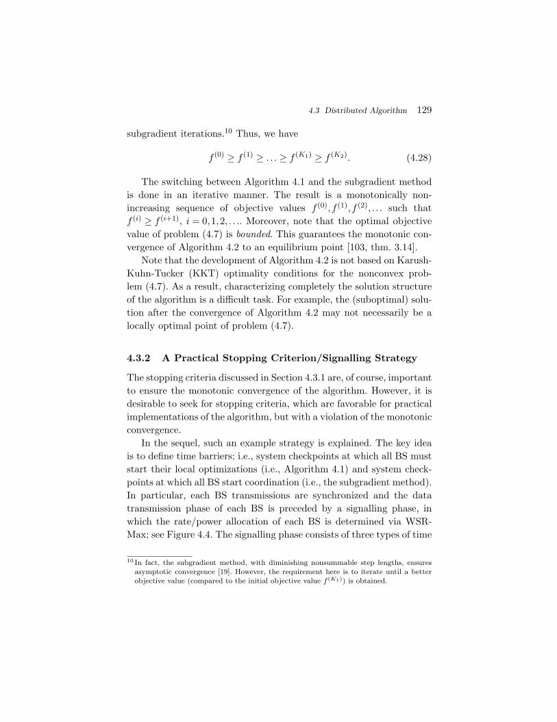
4.3 Distributed Algorithm 129
subgradient iterations.10 Thus, we have
f (0) ≥ f (1) ≥ . . . ≥ f (K1) ≥ f (K2). (4.28)
The switching between Algorithm 4.1 and the subgradient methodis done in an iterative manner. The result is a monotonically non-increasing sequence of objective values f (0),f (1),f (2), . . . such thatf (i) ≥ f (i+1), i = 0,1,2, . . .. Moreover, note that the optimal objectivevalue of problem (4.7) is bounded. This guarantees the monotonic con-vergence of Algorithm 4.2 to an equilibrium point [103, thm. 3.14].
Note that the development of Algorithm 4.2 is not based on Karush-Kuhn-Tucker (KKT) optimality conditions for the nonconvex prob-lem (4.7). As a result, characterizing completely the solution structureof the algorithm is a difficult task. For example, the (suboptimal) solu-tion after the convergence of Algorithm 4.2 may not necessarily be alocally optimal point of problem (4.7).
4.3.2 A Practical Stopping Criterion/Signalling Strategy
The stopping criteria discussed in Section 4.3.1 are, of course, importantto ensure the monotonic convergence of the algorithm. However, it isdesirable to seek for stopping criteria, which are favorable for practicalimplementations of the algorithm, but with a violation of the monotonicconvergence.
In the sequel, such an example strategy is explained. The key ideais to define time barriers; i.e., system checkpoints at which all BS muststart their local optimizations (i.e., Algorithm 4.1) and system check-points at which all BS start coordination (i.e., the subgradient method).In particular, each BS transmissions are synchronized and the datatransmission phase of each BS is preceded by a signalling phase, inwhich the rate/power allocation of each BS is determined via WSR-Max; see Figure 4.4. The signalling phase consists of three types of time
10 In fact, the subgradient method, with diminishing nonsummable step lengths, ensuresasymptotic convergence [19]. However, the requirement here is to iterate until a betterobjective value (compared to the initial objective value f (K1)) is obtained.

130 A Distributed Approach
Fig. 4.4 An example signalling frame structure.
slots called initial signalling window, BS optimization window, and BScoordination window. The initial signalling window is used for step 1of Algorithm 4.2, i.e., the initialization step. The latter two types ofwindows (i.e., BS optimization window and BS coordination window)are repeated until the data transmission phase is reached as shownin Figure 4.4. We define the BS optimization windows to be the timeperiods where Algorithm 4.1 is performed asynchronously. Therefore,during BS optimization windows, step 2 of Algorithm 4.2 is carriedout. The width of the window is determined by the maximum numberof Algorithm 4.1 iterations. The BS coordination windows are definedto be the time periods where the subgradient method is performed.Therefore, during any BS coordination window, step 3, step 4, andstep 5 of Algorithm 4.2 are carried out repeatedly. The width of the BScoordination window is determined by the maximum number of sub-gradient iterations. Typically, we may assume that the time period ofany BS optimization window is significantly smaller compared to thetime period of any BS coordination window because of the followingreasons: (1) significant computing power available at BSs so that the BSoptimization can be performed very fast, (2) BS coordination requirebackhaul message exchanges between BSs, which in turn demand strin-gent time requirements.

4.4 Numerical Examples 131
4.4 Numerical Examples
In this section we run Algorithm 4.2 (Section 4.3) in multiuser multicellenvironments and the benefits due to different degrees of BS coordina-tion are numerically evaluated. As benchmarks, we consider three algo-rithms: (1) distributed WMMSE algorithm [110], (2) GP-SOCP basedcentralized algorithm proposed in [34, sec. 4.3], and (3) the distributedalgorithm proposed in [10, 11], which is based on a ZF beamformingstrategy. To emphasize the practical relevance of the algorithm, weconsider only the stopping criterion discussed in Section 4.3.2, which isbased on time barriers or system checkpoints as shown in Figure 4.4.
We consider an exponential path loss model, where the channelgains between BSs and users are given by
hij =
√(dij
d0
)−η
cij , (4.29)
where dij is the distance from the transmitter of ith data stream tothe receiver of jth data stream, d0 is the far field reference distance[64], η is the path loss exponent, and cij ∈ CT such that cij ∼ CN (0,I)(i.e., frequency-flat fading with uncorrelated antennas). The first termof (4.29) represents the path loss factor and the second term modelsthe Rayleigh small-scale fading. An arbitrarily generated set C of fadingcoefficients where C = {cij | i, j ∈ L} is referred to as a single fadingrealization. The variance of the noise is considered equal for all datastreams, i.e., σ2
l = N0 for all l ∈ L and the maximum power constraintis assumed the same for all nodes, i.e., pmax
n = pmax0 for all n ∈ N . We
define the signal-to-noise ratio (or SNR) operating point at a distanced [distance units] as
SNR(d) =
pmax0N0
d ≤ d0
pmax0N0
(d
d0
)−η
otherwise.(4.30)
In all the simulations we set d0 =1, η=4, pmax0 /N0 =45 dB, SNR
(Rint) = 0 dB, where Rint is the radius of the interference regions of
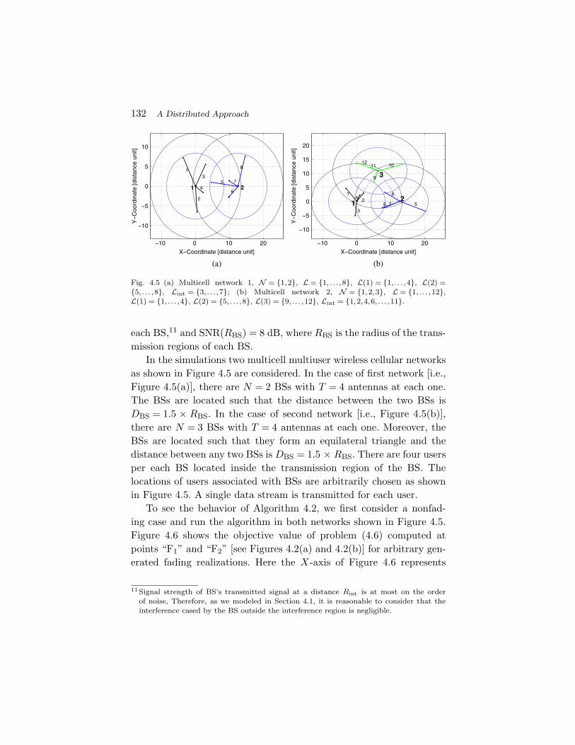
132 A Distributed Approach
−10 0 10 20
−10
−5
0
5
10
X−Coordinate [distance unit]
Y−
Coo
rdin
ate
[dis
tanc
e un
it]
1
2
3
45
6
7
8
1 2
(a)
−10 0 10 20
−10
−5
0
5
10
15
20
X−Coordinate [distance unit]
Y−
Coo
rdin
ate
[dis
tanc
e un
it]
12
3
456, 7
8
9
101112
12
3
(b)
Fig. 4.5 (a) Multicell network 1, N = {1,2}, L = {1, . . . ,8}, L(1) = {1, . . . ,4}, L(2) ={5, . . . ,8}, Lint = {3, . . . ,7}; (b) Multicell network 2, N = {1,2,3}, L = {1, . . . ,12},L(1) = {1, . . . ,4}, L(2) = {5, . . . ,8}, L(3) = {9, . . . ,12}, Lint = {1,2,4,6, . . . ,11}.
each BS,11 and SNR(RBS) = 8 dB, where RBS is the radius of the trans-mission regions of each BS.
In the simulations two multicell multiuser wireless cellular networksas shown in Figure 4.5 are considered. In the case of first network [i.e.,Figure 4.5(a)], there are N = 2 BSs with T = 4 antennas at each one.The BSs are located such that the distance between the two BSs isDBS = 1.5 × RBS. In the case of second network [i.e., Figure 4.5(b)],there are N = 3 BSs with T = 4 antennas at each one. Moreover, theBSs are located such that they form an equilateral triangle and thedistance between any two BSs is DBS = 1.5 × RBS. There are four usersper each BS located inside the transmission region of the BS. Thelocations of users associated with BSs are arbitrarily chosen as shownin Figure 4.5. A single data stream is transmitted for each user.
To see the behavior of Algorithm 4.2, we first consider a nonfad-ing case and run the algorithm in both networks shown in Figure 4.5.Figure 4.6 shows the objective value of problem (4.6) computed atpoints “F1” and “F2” [see Figures 4.2(a) and 4.2(b)] for arbitrary gen-erated fading realizations. Here the X-axis of Figure 4.6 represents
11 Signal strength of BS’s transmitted signal at a distance Rint is at most on the orderof noise, Therefore, as we modeled in Section 4.1, it is reasonable to consider that theinterference cased by the BS outside the interference region is negligible.

4.4 Numerical Examples 133
(a)
(b)
20 40 60 80 100 1208
9
10
11
12
13
14
15
(Algorithm 4.1 iterations + subgradient iterations)
WS
R v
alue
[bits
/sec
/Hz]
WMMSE [110]centralized alg. [34, section 4.3]Alg. 4.2, J
subgrad = 1
Alg. 4.2, Jsubgrad
= 10
Alg. 4.2, Jsubgrad
= 50
distributed alg. [10]
22% Alg. 4.1 subg.Alg. Alg. 4.1 subg.
Alg.
20 40 60 80 100 12018
20
22
24
26
28
30
32
(Algorithm 4.1 iterations + subgradient iterations )
WS
R v
alue
[bits
/sec
/Hz]
WMMSE [110]centralized alg. [34, section 4.3]Alg. 4.2, J
subgrad = 1
Alg. 4.2, Jsubgrad
= 50
distributed alg. [10]
23%
Fig. 4.6 Objective value versus GP iteration: (a) Multicell network 1; (b) Multicellnetwork 2.
combined Algorithm 4.1 iterations and subgradient iterations. For sim-plicity, we denote the number of Algorithm 4.1 iterations carried outduring the BS optimization window by JBS−opt and denote the numberof subgradient iterations performed during the BS coordination windowby Jsubgrad.
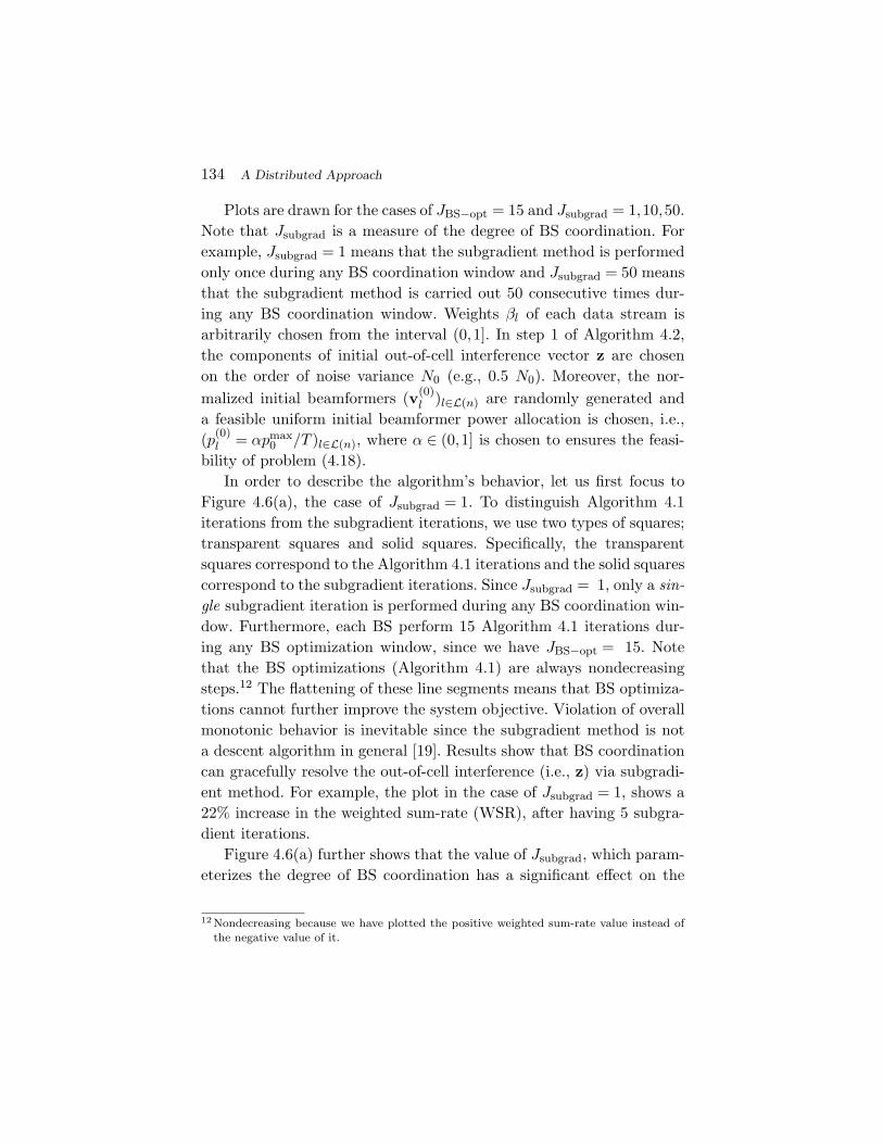
134 A Distributed Approach
Plots are drawn for the cases of JBS−opt = 15 and Jsubgrad = 1,10,50.Note that Jsubgrad is a measure of the degree of BS coordination. Forexample, Jsubgrad = 1 means that the subgradient method is performedonly once during any BS coordination window and Jsubgrad = 50 meansthat the subgradient method is carried out 50 consecutive times dur-ing any BS coordination window. Weights βl of each data stream isarbitrarily chosen from the interval (0,1]. In step 1 of Algorithm 4.2,the components of initial out-of-cell interference vector z are chosenon the order of noise variance N0 (e.g., 0.5 N0). Moreover, the nor-malized initial beamformers (v(0)
l )l∈L(n) are randomly generated anda feasible uniform initial beamformer power allocation is chosen, i.e.,(p(0)
l = αpmax0 /T )l∈L(n), where α ∈ (0,1] is chosen to ensures the feasi-
bility of problem (4.18).In order to describe the algorithm’s behavior, let us first focus to
Figure 4.6(a), the case of Jsubgrad = 1. To distinguish Algorithm 4.1iterations from the subgradient iterations, we use two types of squares;transparent squares and solid squares. Specifically, the transparentsquares correspond to the Algorithm 4.1 iterations and the solid squarescorrespond to the subgradient iterations. Since Jsubgrad = 1, only a sin-gle subgradient iteration is performed during any BS coordination win-dow. Furthermore, each BS perform 15 Algorithm 4.1 iterations dur-ing any BS optimization window, since we have JBS−opt = 15. Notethat the BS optimizations (Algorithm 4.1) are always nondecreasingsteps.12 The flattening of these line segments means that BS optimiza-tions cannot further improve the system objective. Violation of overallmonotonic behavior is inevitable since the subgradient method is nota descent algorithm in general [19]. Results show that BS coordinationcan gracefully resolve the out-of-cell interference (i.e., z) via subgradi-ent method. For example, the plot in the case of Jsubgrad = 1, shows a22% increase in the weighted sum-rate (WSR), after having 5 subgra-dient iterations.
Figure 4.6(a) further shows that the value of Jsubgrad, which param-eterizes the degree of BS coordination has a significant effect on the
12 Nondecreasing because we have plotted the positive weighted sum-rate value instead ofthe negative value of it.

4.4 Numerical Examples 135
overall WSR value. It is interesting to note that, a smaller number ofconsecutive subgradient iterations (e.g., Jsubgrad = 1,10) can performbetter compared to a larger number of consecutive subgradient itera-tions (e.g., Jsubgrad = 50). Such a behavior is very important in prac-tice to reduce significantly the backhaul message exchanges during anyBS coordination window. We can intuitively explain the behavior byconsidering the two points “A” and “B” in Figure 4.3(a). In partic-ular, point “A” corresponds to a smaller Jsubgrad, where the (convexform) approximated master problem (4.21) is solved to a low accu-racy. Point “B” corresponds to a larger Jsubgrad, where the (convexform) approximated master problem is solved to a high accuracy. Ofcourse, point “B” is better than point “A” for the approximated mas-ter problem, but not necessarily for the original master problem (4.9);see the master objective depicted in Figure 4.3(a). This suggest thatone need not solve each approximation to a high accuracy. Refining theapproximation more often (which corresponds to a smaller Jsubgrad),rather than solving some approximated master problem to a high accu-racy (which corresponds to a larger Jsubgrad) is more beneficial.
Figure 4.6(b) shows the algorithm behavior in the case of networksetup 2 in Figure 4.5(b). The behavior is very similar to the previ-ous plots in Figure 4.6(a). The network can yield substantial gains byperforming just one subgradient iterations during any BS coordinationwindow, that is, less backhaul message exchanges between BSs. Forexample, the plot in the case of Jsubgrad = 1, shows a 23% increasein the WSR, after having 5 subgradient iterations; see Figure 4.6(a).Figure 4.6 also shows the performance of the considered benchmarkalgorithms after their convergence. In both networks, for the consid-ered channel realizations, the performance of the distributed algorithmin [10] is significantly low. It is intuitively clear that the performancedrop is due to the lack of degrees of freedom available at BS transmis-sions to avoid interference. Results further show that the distributedWMMSE algorithm outperforms Algorithm 4.2 in both scenarios. Suchresults are intuitively expected because WMMSE algorithm do relyon user terminal assistance during algorithm’s iterations compared toAlgorithm 4.2. The good performance of the centralized algorithmcompared to Algorithm 4.2 agrees with the intuition that methods
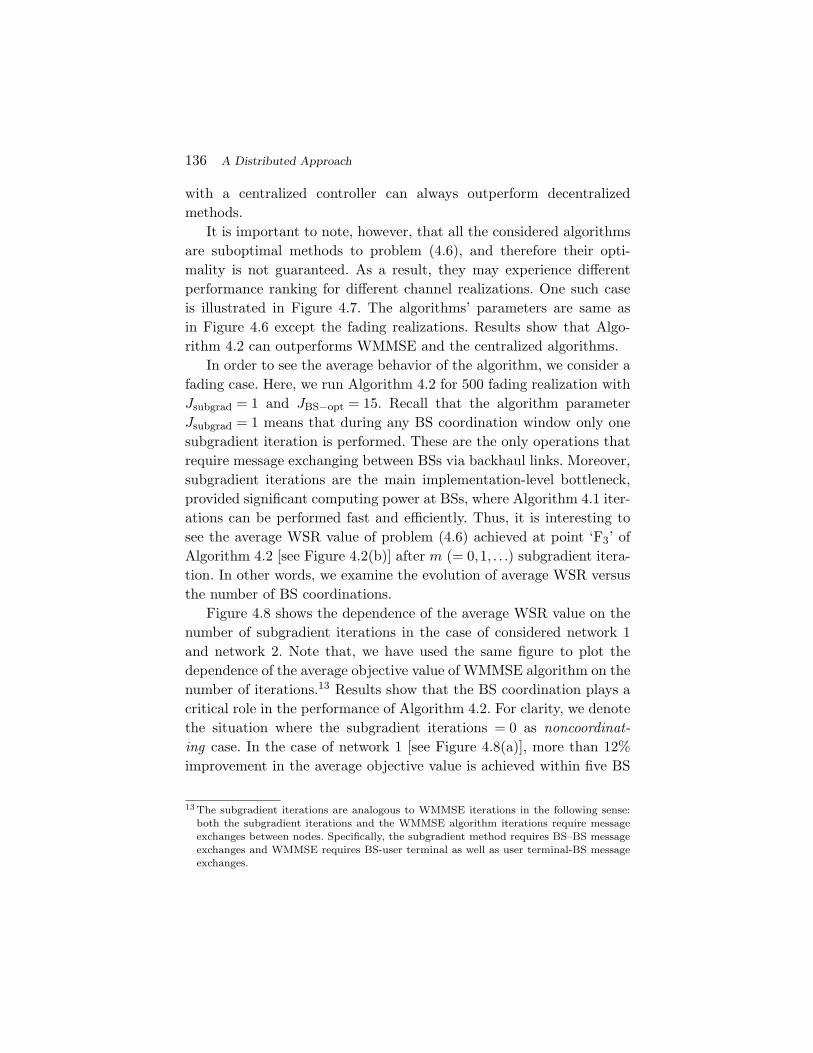
136 A Distributed Approach
with a centralized controller can always outperform decentralizedmethods.
It is important to note, however, that all the considered algorithmsare suboptimal methods to problem (4.6), and therefore their opti-mality is not guaranteed. As a result, they may experience differentperformance ranking for different channel realizations. One such caseis illustrated in Figure 4.7. The algorithms’ parameters are same asin Figure 4.6 except the fading realizations. Results show that Algo-rithm 4.2 can outperforms WMMSE and the centralized algorithms.
In order to see the average behavior of the algorithm, we consider afading case. Here, we run Algorithm 4.2 for 500 fading realization withJsubgrad = 1 and JBS−opt = 15. Recall that the algorithm parameterJsubgrad = 1 means that during any BS coordination window only onesubgradient iteration is performed. These are the only operations thatrequire message exchanging between BSs via backhaul links. Moreover,subgradient iterations are the main implementation-level bottleneck,provided significant computing power at BSs, where Algorithm 4.1 iter-ations can be performed fast and efficiently. Thus, it is interesting tosee the average WSR value of problem (4.6) achieved at point ‘F3’ ofAlgorithm 4.2 [see Figure 4.2(b)] after m (= 0,1, . . .) subgradient itera-tion. In other words, we examine the evolution of average WSR versusthe number of BS coordinations.
Figure 4.8 shows the dependence of the average WSR value on thenumber of subgradient iterations in the case of considered network 1and network 2. Note that, we have used the same figure to plot thedependence of the average objective value of WMMSE algorithm on thenumber of iterations.13 Results show that the BS coordination plays acritical role in the performance of Algorithm 4.2. For clarity, we denotethe situation where the subgradient iterations = 0 as noncoordinat-ing case. In the case of network 1 [see Figure 4.8(a)], more than 12%improvement in the average objective value is achieved within five BS
13 The subgradient iterations are analogous to WMMSE iterations in the following sense:both the subgradient iterations and the WMMSE algorithm iterations require messageexchanges between nodes. Specifically, the subgradient method requires BS–BS messageexchanges and WMMSE requires BS-user terminal as well as user terminal-BS messageexchanges.
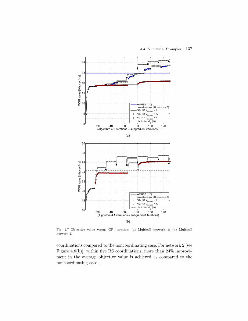
4.4 Numerical Examples 137
(a)
(b)
20 40 60 80 100 1208
9
10
11
12
13
14
(Algorithm 4.1 iterations + subgradient iterations )
WS
R v
alue
[bits
/sec
/Hz]
WMMSE [110]centralized alg. [34, section 4.3]Alg. 4.2, J
subgrad = 1
Alg. 4.2, Jsubgrad
= 10
Alg. 4.2, Jsubgrad
= 50
distributed alg. [10]
20 40 60 80 100 12016
18
20
22
24
26
28
30
(Algorithm 4.1 iterations + subgradient iterations)
WS
R v
alue
[bits
/sec
/Hz]
WMMSE [110]centralized alg. [34, section 4.3]Alg. 4.2, J
subgrad = 1
Alg. 4.2, Jsubgrad
= 50
distributed alg. [10]
Fig. 4.7 Objective value versus GP iteration: (a) Multicell network 1; (b) Multicellnetwork 2.
coordinations compared to the noncoordinating case. For network 2 [seeFigure 4.8(b)], within five BS coordinations, more than 24% improve-ment in the average objective value is achieved as compared to thenoncoordinating case.
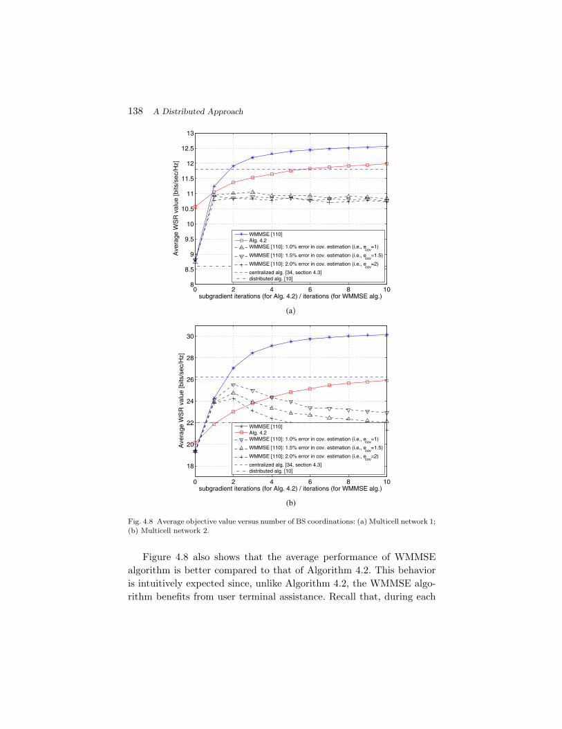
138 A Distributed Approach
(a)
(b)
0 2 4 6 8 108
8.5
9
9.5
10
10.5
11
11.5
12
12.5
13
subgradient iterations (for Alg. 4.2) / iterations (for WMMSE alg.)
Ave
rage
WS
R v
alue
[bits
/sec
/Hz]
WMMSE [110]Alg. 4.2WMMSE [110]: 1.0% error in cov. estimation (i.e., e
cov=1)
WMMSE [110]: 1.5% error in cov. estimation (i.e., ecov
=1.5)
WMMSE [110]: 2.0% error in cov. estimation (i.e., ecov
=2)
centralized alg. [34, section 4.3]distributed alg. [10]
0 2 4 6 8 10
18
20
22
24
26
28
30
subgradient iterations (for Alg. 4.2) / iterations (for WMMSE alg.)
Ave
rage
WS
R v
alue
[bits
/sec
/Hz]
WMMSE [110]Alg. 4.2WMMSE [110]: 1.0% error in cov. estimation (i.e., e
cov=1)
WMMSE [110]: 1.5% error in cov. estimation (i.e., ecov
=1.5)
WMMSE [110]: 2.0% error in cov. estimation (i.e., ecov
=2)
centralized alg. [34, section 4.3]distributed alg. [10]
Fig. 4.8 Average objective value versus number of BS coordinations: (a) Multicell network 1;(b) Multicell network 2.
Figure 4.8 also shows that the average performance of WMMSEalgorithm is better compared to that of Algorithm 4.2. This behavioris intuitively expected since, unlike Algorithm 4.2, the WMMSE algo-rithm benefits from user terminal assistance. Recall that, during each

4.5 Summary and Discussion 139
iterations, WMMSE algorithm requires user terminals assistance suchas signal covariance estimations, computations, and feedback informa-tion to BSs over the air interface. In contrast, the given method requireonly BS-level synchronized communication and all the necessary com-putation is concentrated at the BSs. The result is naturally a tradeoff between performance gains and the implementation-level simplic-ity. For a fair comparison of Algorithm 4.2 and WMMSE algorithm,we examine the sensitivity of WMMSE algorithm to imperfections onthe signal covariance estimations at user terminals. Specifically, dur-ing each WMMSE iteration, we randomly perturb the error free signalcovariance matrix Jl (which is a scalar in the case of MISO) at eachuser terminal l as follows: Jl = Jl + Jl(xecov/100), where x is a randomvariable with 2 equiprobable outcomes −1,1 and ecov is the amountof covariance perturbation. Results show that such small estimationerrors have a significant effect on the performance of WMMSE algo-rithm. Moreover, in such situations, the convergence of the WMMSEmethod becomes less predictable. Thus, the algorithm presented is wellsuited for systems where the user terminal assistance is not desirabledue to potential errors such as estimation errors and feedback errors.
Figure 4.8 further shows that, the performance of Algorithm 4.2within several BS coordinations is comparable with that of the cen-tralized algorithm [34, sec. 4.3]. For example, in the case of network 1,Algorithm 4.2 achieves around 99% of the average WSR value givenby the centralized algorithm [34, sec. 4.3]. Moreover, in the case ofnetwork 2, Algorithm 4.2 yields around 94% of the average WSR valuegiven by the considered centralized algorithm. Finally, we see that thereis a substantial performance gap between Algorithm 4.2 and the dis-tributed algorithm in [10]. The main reason for such a performancedrop of algorithm in [10] is the insufficient degree of freedom availableat BS transmissions to cancel the interference it causes to the userterminals.
4.5 Summary and Discussion
The weighted sum-rate maximization problem in a multicell multiple-input and single-output downlink system was considered. The problem
140 A Distributed Approach
is nonconvex; in fact it is NP-hard. A distributed solution methodfor the problem was presented. The main advantage of the givendistributed algorithm is its implementation-level simplicity. Unlike theminimum weighted mean-squared error based algorithms, the methodpresented does not demand user terminal assistance during eachiteration. It essentially requires base station to base station (BS) com-munication, which are reasonably realizable, provided reliable backhaullinks (e.g., fibre and microwave links) and significant computing powerat BSs. As a result, a good trade-off between the performance gainsand the implementation-level simplicity was achieved. The algorithmwas based on primal decomposition and subgradient methods. Inparticular, the main problem was split into a master problem andmany subproblems (one for each base station). A sequential convexapproximation strategy together with a subgradient method were blentto address the nonconvex master problem. Master problem solutionrelies on synchronous BS coordinations. A descent algorithm based onsecond-order cone programming and a geometric programming wereadopted in the case of subproblems. The subproblems can be performedin a fully asynchronous manner. The monotonic convergence of thealgorithm was established, with appropriate choice of stopping criteriaat intermediate steps. Practical stopping criteria were also presented.Numerical experiments were presented to compare the method withother state-of-the-art algorithms. Results suggest that the algorithmis well suited for systems where the user terminal assistance is notallowed or not desirable. Results further showed that the algorithmcould significantly improve the overall system performance with asmall amount of BS coordinations. These observations are indeedimportant for deriving simple signalling protocols in the context oflarge-scale practical cellular communication systems.

5Conclusions
In this volume a greater emphasis was placed on the general weightedsum-rate maximization (WSRMax) problem, which is NP-hard; it playsan important role in various problems of recent interest in wireless com-munication, including network utility maximization, cross-layer design,link scheduling, and many others.
The first section was mainly intended to highlight the motivationfor the WSRMax problem and to review earlier and parallel work. InSection 2, a global optimization approach based on the branch andbound technique was presented to solve the nonconvex WSRMax prob-lem with an optimality certificate. Efficient analytic bounding methodswere given and their effect on the convergence of the branch and boundalgorithm was analyzed numerically. Though the convergence speed wasdramatically increased by improving the lower bound, the benefits ofimproving the upper bounding methods are imperceptible. This sug-gests that a grater emphasis should be placed on exploring better lowerbounding techniques. Unlike other branch and bound based algorithmsfor WSRMax, the method presented does not rely on the convertibilityof the problem into a DC (difference of convex functions) problem.Therefore, the method applies to a broader class of WSRMax problems
141

142 Conclusions
(e.g., WSRMax in multicast wireless networks). More importantly, itcan address any system performance metric that can be expressed as aLipschitz continuous and increasing function of signal-to-interference-plus-noise ratio (SINR) values (not restricted to WSRMax).
The worst case complexity of the branch and bound algorithmincreases exponentially with the problem size for a given accuracy. Evena small-scale problems (e.g., one with few tens of variables) can takea long time, and therefore such global methods are applicable whenthe computing time requirements are not critical. This means that,in the case of wireless networks, where the computing time is oftencrucial, any global optimization method is hardly applicable. However,it is indeed useful to provide performance benchmarks, e.g., for evalu-ating the performance loss encountered by any suboptimal method forWSRMax.
The link-interference model considered in Section 2 is very general;it accommodates a wide variety of network topologies. Moreover, theconsidered link-interference model supports different node capabilities,including single- or multipacket transmission, single- or multipacketreception, and many others. Numerical examples of diverse applicationdomains of WSRMax were presented to demonstrate the branch andbound algorithm.
Fast, suboptimal algorithms for the WSRMax problem in generalmulticommodity, multichannel wireless networks were considered inSection 3. The algorithms were used within a general cross-layer util-ity maximization framework and the quantitative impact of gains thatcan be achieved at the network layer in terms of end-to-end rates andnetwork congestion was numerically evaluated.
First, a general access operation with a relatively simple form ofreceivers structure (a bank of match filters) was considered; a receiverdecodes each of its intended signals by treating all other interfering sig-nals as noise. The presented algorithms were based on complementarygeometric programming and homotopy methods. The algorithm basedon homotopy methods handled the self-interference problem withoutcombinatorial constraints to enforce simultaneous transmissions andreceptions in the same frequency band; thus the combinatorial natureof the problem has been circumvented. Numerical results showed that

143
the algorithms could exploit the multichannel diversity via dynamicpower allocation across the available channels. It was interesting tosee numerically that they performed closely to the exponentially com-plex optimal branch and bound algorithm. The methods also provide amechanism, based on which the gains achievable at the network layercould be evaluated when the network nodes employ self interferencecancelation techniques with different degrees of accuracy. Numericalresults showed that quantifiable gains at the network layer have beenachieved after a certain level of the self interference cancelation accu-racy, e.g., a self interference reduction in the range 20−60 dB led tosignificant gains at the network layer.
The latter part of Section 3 considered a case where all receiversperform multiuser detection and the gains that can be achieved at thenetwork layer were numerically evaluated. The solution methods herewere obtained by imposing additional constraints, such as that onlyone node can transmit to others at a time or that only one node canreceive from others at a time. The main benefit of such constraintswas the problem tractability and simplicity of the solution methods.Consequently, these simple access protocols can be potentially usefulin practice with more advanced communication systems.
Note that all the algorithms presented in Section 3 are reliant onthe well known interior-point methods. Therefore, the algorithms arefast, compared to the optimal branch and bound algorithm presented inSection 2 and they can be deployed in relatively large-scale problems(e.g., one with few hundreds of variables), which are not, of course,apparently handled by exponentially complex optimal algorithms. How-ever, to facilitate the use of the algorithms in real-time applicationsfurther improvements in the efficiency are required. There are manyimportant issues and methods in linear algebra that can be used toimprove the efficiency of the algorithms. For example, the structure ofthe problem can be heavily exploited. We may assume in a wirelessnetwork that, the problem variables (e.g., power and SINRs) are notfully coupled due to exponential path losses. Such assumptions, whichare reasonable in practice, can result desirable sparsity patterns of theinvolved problem data (e.g., sparse matrices), and can dramaticallyincrease the efficiency of the methods.

144 Conclusions
An easy to implement distributed method for WSRMax problemin a multicell multiple antenna downlink system was presented inSection 4. Unlike the recently proposed minimum weighted mean-squared error based algorithms, where at each iteration all mobileterminals needs to estimate the covariance matrices of their receivedsignals, compute and feedback over the air certain parameters to thebase stations (BS), the presented algorithm operates without anyuser terminal assistance. It requires only BS to BS signalling viareliable backhaul links (e.g. fiber, microwave links) and all requiredcomputation is performed at the BSs. The algorithm is based on primaldecomposition and subgradient methods, where the original nonconvexproblem is split into a master problem and a number of subproblems(one for each BS). A sequential convex approximation strategywas used to address the nonconvex master problem. In the case ofsubproblems, an existing iterative approach based on second-ordercone programming and geometric programming was adopted. Thesubproblems were coordinated to find a (possibly suboptimal) solutionto the master problem. Subproblems can be solved by BSs in a fullyasynchronous manner, though the coordination between subproblemsshould be synchronous. Numerical results were provided to see thebehavior of the algorithm under different degrees of BS coordination.They showed that the algorithm could yield a good tradeoff betweenthe implementation-level simplicity and the performance.

AImproving Upper Bound for Branch
and Bound via ComplementaryGeometric Programming
We show in this appendix how to compute efficiently γImpCGP viaCGP [6], when f0(γ) =
∑l∈L −βl log(1 + γl). Note that this is the only
place where the exact expression of the rate function (2.1) has beenexplicitly taken into account. In the derivation of all other bounds onlythe monotonicity property has been used. We start by equivalentlyreformulating problem (2.48) as
minimize∏
l∈L(1 + γl
)−βl
subject to γl,min ≤ γl ≤ γl,max, l ∈ L
γl ≤ gllpl
σ2 +∑
j �=l gjlpj, l ∈ L
∑l∈O(n) pl ≤ pmax
n , n ∈ Tpl ≥ 0, l ∈ L,
(A.1)
where the variables are (pl)l∈L and (γl)l∈L. The equivalence betweenproblem (2.48) and problem (A.1) follows from the monotonicallyincreasing property of log(·) function and the explicit description of the
145

146 Improving Upper Bound for Branch and Bound
constraints. To obtain a suboptimal solution, we adopt Algorithm 3.2(see Section 3.2.2) in a straightforward manner as follows:
Algorithm A.0.1 CGP based algorithm for finding γImpCGP
1. Given tolerance ε > 0. Let γ = al� .2. Solve the following GP:
minimize∏
l∈L γl−βl
γl1+γl
subject to γl,min ≤ γl ≤ γl,max, l ∈ L
γl ≤ gllpl
σ2 +∑
j �=l gjlpj, l ∈ L∑
l∈O(n) pl ≤ pmaxn , n ∈ T ,
(A.2)
with the variables (pl)l∈L and (γl)l∈L. Denote the solution by(p�
l )l∈L and (γ�l )l∈L.
3. If maxl∈L |γ�l − γl| > ε set (γl = γ�
l )l∈L and go to step 2. Oth-erwise set γImpCGP = γ and STOP.

BThe Barrier Method
In this appendix we outline the basic steps involved in solvingproblem (3.33) using the barrier method [22, sec. 11.3.1]. For thesake of notational simplicity let us define σρn(k) = σ2/gρn(k)ρn(k) fork = 1, . . . , |O(n)| and σρn(|O(n)|+1) = 0. Furthermore, let ui be the ith
column of the upper triangular matrix U ∈ IR|O(n)|×|O(n)|+ with all
nonzero entries being equal to 1.By denoting the feasible set of rate allocation vector rn =
(rρn(1) . . . rρn(|O(n)|)) [125, sec. 3], problem (3.33) can be equivalentlyexpressed as
maximize∑
l∈O(n) βlrl
subject to ui(rn) ≤ 0, i = 1, . . . , |O(n)| + 1,(B.1)
where the variable is rn. The function ui(rn) can be compactlyexpressed as
ui(rn) =
−eTi rn 1 ≤ i ≤ |O(n)|
|O(n)|∑j=1
bn(j)euTj rn − σρn(1) − pmax
n i = |O(n)| + 1,
147
148 The Barrier Method
where bn(j) = σρn(j) − σρn(j+1). Problem (B.1) is a convex optimizationproblem [22], and therefore can be solved efficiently. It is worth notingthat, given any feasible rn the corresponding power variables pρn(k),k = 1, . . . , |O(n)| are given by [125]
pρn(k) = (erρn(k) − 1)∑i≥k
bn(i)e∑
k<j≤i rρn(j) .
The barrier method [22, sec. 11.3.1] can be used to solve problem (B.1).The gradient and the Hessian of the function ui(rn) are given by
∇ui(rn) =
{−ei 1 ≤ i ≤ |O(n)|∑|O(n)|
j=1 bn(j)euTj rnuj i = |O(n)| + 1
and
∇2ui(rn) =
{0 1 ≤ i ≤ |O(n)|∑|O(n)|
j=1 bn(j)euTj rnujuT
j i = |O(n)| + 1.
The expressions above are used to evaluate the gradient and the Hessianof the logarithmic barrier function [22, sec. 11.2.1].

Acknowledgments
The work of P.C. Weeraddana and C. Fischione was supported by theSwedish Research Council and EU projects Hydrobionets and Hycon2.Most of the results have been obtained during Dr. Weeraddan’s doc-toral studies at the University of Oulu, Finland. M. Codreanu andM. Latva-aho were supported by the Finnish Funding Agency forTechnology and Innovation (Tekes), Academy of Finland, Nokia,Nokia Siemens Networks, Renesas Mobile Europe, and Elektrobit.A. Ephremides was supported by the NSF grant CCF-0728966,CCF-0905209, and US Army Research Office grant W911NF-08-1-0238.
149
Notations and Acronyms
E{·} Expectationei ith standard unit vectorI Identity matrix; size of the matrix is implicit1 Vector of 1s, i.e., (1, . . . ,1); size of the vector is implicit|x| Absolute value of the complex number x
||x||2 �2-norm of complex vector xXH Conjugate transpose (Hermtian) of matrix XXT Transpose of matrix XX−1 Inverse of matrix X[X]i,j Element at the ith row and the jth column of matrix X|X | Cardinality of set X∇f(x) Gradient of function f at x∇2f(x) Hessian matrix of function f at xC Set of complex numbersCn Set of complex n-vectorsCm×n Set of complex m × n matrices
150

Notations and Acronyms 151
IR,IR+,IR++ Set of real, and nonnegative real numbersIRn
+ Cone of nonnegative, real n-vectorsIRm×n
+ Set of nonnegative, real m × n matricesCN (m,K) Circularly symmetric complex Gaussian vector
distribution with mean m and covariance matrix K∼ Distributed according to≥ Greater than or equal operator; between real
matrices, it represents componentwise inequality
CGP Complementary Geometric ProgrammingGP Geometric ProgrammingMWM MaxWeight MatchingNUM Network Utility MaximizationRA Resource AllocationSINR Signal-To-Interference-Plus-Noise RatioSNR Signal-To-Noise RatioSOCP Second-Order Cone ProgrammingSP Signomial ProgrammingWSR Weighted Sum-RateWSRMax Weighted Sum-Rate Maximization

References
[1] I. C. Abou-Faycal, M. D. Trott, and S. Shamai, “The capacity of discrete-timememoryless Rayleigh-fading channels,” IEEE Transaction on InformationTheory, vol. 47, no. 4, pp. 1290–1301, May 2001.
[2] R. Agarwal and J. M. Cioffi, “Beamforming design for the MIMO downlinkfor maximizing weighted sum-rate,” in Proceedings on IEEE InternationalSymposium on Information Theory and its Applications, pp. 1–6, Auckland,New Zealand, December 7–10 2008.
[3] H. Al-Shatri and T. Weber, “Optimizing power allocation in interference chan-nels using D.C. programming,” in Proceedings on Workshop on Resource Allo-cation in Wireless Networking, pp. 367–373, Avignon, France, June 4 2010.
[4] E. L. Allgower and K. Georg, Introduction to Numerical Continuation Meth-ods. Philadelphia, PA: SIAM, 2003.
[5] C. Audet, P. Hansen, and G. Savard, Essays and Surveys in Global Optimiza-tion. 233 Spring street, NY 10013, USA: Springer Science + Business Media,Inc, 2005.
[6] M. Avriel and A. C. Williams, “Complementary geometric programming,”SIAM Journal on Appllied Mathematics, vol. 19, no. 1, pp. 125–141, July1970.
[7] C. Bae and D. Cho, “Fairness-aware adaptive resource allocation scheme inmultihop OFDMA systems,” IEEE Communications Letters, vol. 11, no. 2,pp. 134–136, February 2007.
[8] V. Balakrishnan, S. Boyd, and S. Balemi, “Branch and bound algorithm forcomputing the minimum stability degree of parameter-dependent linear sys-tems,” International Journal on Robust and Nonlinear Control, vol. 1, no. 4,pp. 295–317, October–December 1991.
152
References 153
[9] D. E. Barreto and S. S. Chiu, “Decomposition methods for cross-layer opti-mization in wireless networks,” in Proceedings on IEEE Wireless Communica-tions and Networking Conference, pp. 270–275, Kawloon, Hong Kong, March11–15 2007.
[10] E. Bjornson, M. Bengtsson, and B. Ottersten, “Optimality properties and low-complexity solutions to coordinated multicell transmission,” in Proceedings onIEEE Global Telecommunications Confernce, pp. 1–6, Miami, Florida, USA,December 6–10 2010.
[11] E. Bjornson, N. Jalden, M. Bengtsson, and B. Ottersten, “Optimality proper-ties, distributed strategies, and measurement-based evaluation of coordinatedmulticell OFDMA transmission,” IEEE Transactions on Signal Processing,vol. 59, no. 12, pp. 6086–6101, December 2011.
[12] E. Bjornson, R. Zakhour, D. Gesbert, and B. Ottersten, “Cooperative mul-ticell precoding: Rate region characterization and distributed strategies withinstantaneous and statistical CSI,” IEEE Transactions on Signal Processing,vol. 58, no. 8, pp. 4298–4310, August 2010.
[13] S. A. Borbash and A. Ephremides, “The feasibility of matchings in a wirelessnetwork,” IEEE Transactions on Information Theory, vol. 52, no. 6, pp. 2749–2755, June 2006.
[14] S. A. Borbash and A. Ephremides, “Wireless link scheduling with powercontrol and SINR constraints,” IEEE Transactions on Information Theory,vol. 52, no. 11, pp. 5106–5111, November 2006.
[15] S. Boyd, “GGPLAB: A simple matlab toolbox for geometric programming,”[Online]. Available: http://www.stanford.edu/∼boyd/ggplab/, 2006.
[16] S. Boyd, “Branch-and-bound methods,” [Online]. Available: http://www.stanford.edu/class/ee364b/lectures/bb slides.pdf, 2007.
[17] S. Boyd, “Primal and dual decomposition,” [Online]. Available: http://www.stanford.edu/class/ee364b/lectures/decomposition slides.pdf, 2007.
[18] S. Boyd, “Sequential convex programming,” [Online]. Available: http://www.stanford.edu/class/ee364b/lectures/seq slides.pdf, 2007.
[19] S. Boyd, “Subgradient methods,” [Online]. Available: http://www.stanford.edu/class/ee364b/lectures/subgrad method slides.pdf, 2007.
[20] S. Boyd, S. J. Kim, L. Vandenberghe, and A. Hassibi, “A tutorial on geometricprogramming,” Optimization and Engineering, vol. 8, no. 1, pp. 67–127, 2007.
[21] S. Boyd, N. Parikh, E. Chu, B. Peleato, and J. Eckstein, “Distributed opti-mization and statistical learning via the alternating direction method ofmultipliers,” Foundations and Trends in Machine Learning, vol. 3, no. 1,pp. 1–122, 2010.
[22] S. Boyd and L. Vandenberghe, Convex Optimization. Cambridge, UK:Cambridge University Press, 2004.
[23] S. Boyd and L. Vandenberghe, “Additional exercises for convex optimization,”[Online]. Available: http://www.stanford.edu/∼boyd/cvxbook/bv cvxbookextra exercises.pdf, May 2010.
[24] L. Bui, A. Eryilmaz, R. Srikant, and X. Wu, “Asynchronous congestion con-trol in multi-hop wireless networks with maximal matching-based scheduling,”IEEE/ACM Transactions on Networking, vol. 16, no. 4, pp. 826–839, August2008.
154 References
[25] M. Cao, V. Raghunathan, S. Hanly, V. Sharma, and P. R. Kumar, “Powercontrol and transmission scheduling for network utility maximization in wire-less networks,” in Proceedings on IEEE International Conference on Decisionand Control, pp. 5215–5221, New Orleans, LA, USA, December 12–14 2007.
[26] M. Cao, X. Wang, S. Kim, and M. Madihian, “Multi-hop wireless backhaulnetworks: A cross-layer design paradigm,” IEEE Journal on Selected Areas inCommunications, vol. 25, no. 4, pp. 738–748, May 2007.
[27] R. Cendrillon, J. Huang, M. Chiang, and M. Moonen, “Autonomous spectrumbalancing for digital subscriber lines,” IEEE Transactions on Signal Process-ing, vol. 55, no. 8, pp. 4241–4257, August 2007.
[28] R. Cendrillon, W. Yu, M. Moonen, J. Verlinden, and T. Bostoen, “Optimalmultiuser spectrum balancing for digital subscriber lines,” IEEE Transactionson Communications, vol. 54, no. 5, pp. 922–933, May 2006.
[29] M. Chiang, “Balancing transport and physical layers in wireless multihop net-works: Jointly optimal congestion control and power control,” IEEE Journalon Selected Areas in Communications, vol. 23, no. 1, pp. 104–116, January2005.
[30] M. Chiang, “Geometric programming for communication systems,” vol. 2,no. 1-2, pp. 1–154, July 2005.
[31] M. Chiang, C. W. Tan, D. P. Palomar, D. O’Neill, and D. Julian, “Powercontrol by geometric programming,” IEEE Transactions on Wireless Com-munications, vol. 6, no. 7, pp. 2640–2651, July 2007.
[32] J. I. Choi, M. Jain, K. Srinivasan, P. Levis, and S. Katti, “Achieving singlechannel, full duplex wireless communication,” in Proceedings on ACM Inter-national Conference on Mobile Computing and Networking, pp. 1–12, Chicago,Illinois, USA, September 20–24 2010.
[33] S. S. Christensen, R. Agarwal, E. Carvalho, and J. Cioffi, “Weighted sum-ratemaximization using weighted MMSE for MIMO-BC beamforming design,”IEEE Transactions on Wireless Communications, vol. 7, no. 12, pp. 4792–4799, December 2008.
[34] M. Codreanu, “Multidimensional adaptive radio links for broadband com-munications,” Ph.D. thesis, Centre for Wireless Communications, Universityof Oulu, Oulu, Finland: Acta Universitatis Ouluensis, [Online]. Available:http://herkules.oulu.fi/isbn9789514286223, November 2007.
[35] M. Codreanu, A. Tolli, M. Juntti, and M. Latva-aho, “Joint design of Tx-Rx beamformers in MIMO downlink channel,” IEEE Transactions on SignalProcessing, vol. 55, no. 9, pp. 4639–4655, September 2007.
[36] T. M. Cover and J. A. Thomas, Elements of Information Theory. New York,USA: John Wiley, second Edition, 2006.
[37] R. L. Cruz and A. V. Santhanam, “Optimal routing, link scheduling and powercontrol in multi-hop wireless networks,” in Proceedings on IEEE INFOCOM,vol. 1, pp. 702–711, San Diego, CA, April 2003.
[38] T. ElBatt and A. Ephremides, “Joint scheduling and power control for wirelessad hoc networks,” IEEE Transactions on Wireless Communications, vol. 3,no. 1, pp. 74–85, January 2004.

References 155
[39] K. Eriksson, “Dynamic resource allocation in wireless networks,” Exa-mensarbete utfort i Kommunikationssystem vid Tekniska hogskolan iLinkoping, [Online]. Available: http://liu.diva-portal.org/smash/get/diva2:326290/FULLTEXT01, 2010.
[40] A. Eryilmaz and R. Srikant, “Fair resource allocation in wireless networksusing queue-length-based scheduling and congestion control,” IEEE/ACMTransactions on Networking, vol. 15, no. 6, pp. 1333–1344, December 2007.
[41] A. Eryilmaz, R. Srikant, and J. R. Perkins, “Stable scheduling policies forfading wireless channels,” IEEE/ACM Transactions on Networking, vol. 13,no. 2, pp. 411–424, April 2005.
[42] A. V. Fiacco, Introduction to Sensitivity and Stability Analysis in NonlinearProgramming, vol. 165. 111 Fifth Avenue, New York, New York 10003: Aca-demic Press, Inc., 1983.
[43] L. Georgiadis, M. J. Neely, and L. Tassiulas, “Resource allocation and cross-layer control in wireless networks,” Foundations and Trends in Networks,vol. 1, no. 1, pp. 1–144, April 2006.
[44] P. Gupta and P. R. Kumar, “The capacity of wireless networks,” IEEE Trans-actions on Information Theory, vol. 46, no. 2, March 2000.
[45] C. Guthy, W. Utschick, R. Hunger, and M. Joham, “Efficient weighted sumrate maximization with linear precoding,” IEEE Transactions on Signal Pro-cessing, vol. 58, no. 4, pp. 2284–2297, April 2010.
[46] B. Hajek and G. Sasaki, “Link scheduling in polynomial time,” IEEE Trans-actions on Information Theory, vol. 34, no. 5, pp. 910–917, September 1988.
[47] D. Halperin, T. Anderson, and D. Wetherall, “Taking the sting out of carriersense: Interference cancellation for wireless LANs,” in Proceedings on ACMInternational conference on Mobile Computing and Networking, pp. 339–350,San Francisco, California, USA, September 14–19 2008.
[48] S. V. Hanly and D. N. C. Tse, “Multiaccess fading channels — Part II: Delay-limited capacities,” IEEE Transactions on Information Theory, vol. 44, no. 7,pp. 2816–2831, November 1998.
[49] Z. K. M. Ho and D. Gesbert, “Balancing egoism and altruism on the MIMOinterference channel,” IEEE Journal on Selected Areas in Communications,submitted, 2010, [Online]. Available: http://arxiv.org/PS cache/arxiv/pdf/0910/0910.1688v1.pdf.
[50] L. M. C. Hoo, B. Halder, J. Tellado, and M. Cioffi, “Multi user transmitoptimization for multiuser broadcast channels: Asymptotic fdma capacityregion and algorithms,” IEEE Transactions on Communications, vol. 52, no. 6,pp. 922–930, June 2004.
[51] R. A. Horn and C. R. Johnson, Topics in Matrix Analysis. Cambridge, UK:Cambridge University Press, 1994.
[52] R. Horst, P. Pardolos, and N. Thoai, Introdiction to Global Optimization,vol. 48. Dordrecht, Boston, London: Kluwer Academic Publishers, secondEdition, 2000.
[53] J. Huang, R. Berry, and M. Honig, “Distributed interference compensationfor wireless networks,” IEEE Journal on Selected Areas in Communications,vol. 24, no. 5, pp. 1074–1084, May 2006.

156 References
[54] J. Jang and K. B. Lee, “Transmit power adaptation for multiuser OFDMsystems,” IEEE Journal on Selected Areas in Communications, vol. 21, no. 2,pp. 171–178, February 2003.
[55] E. A. Jorswieck and E. G. Larsson, “The MISO interference channel from agame-theoretic perspective: A combination of selfishness and altruism achievespareto optimality,” in Proceedings on IEEE International Conference onAcoustics, Speech, Signal Processing, pp. 5364–5367, Las Vegas, Nevada, USA,March 31–April 4 2008.
[56] E. A. Jorswieck, E. G. Larsson, and D. Danev, “Complete characterization ofthe pareto boundary for the MISO interference channel,” IEEE Transactionson Signal Processing, vol. 56, no. 10, pp. 5292–5296, October 2008.
[57] S. Joshi, P. C. Weeraddana, M. Codreanu, and M. Latva-aho, “Weighted Sum-Rate Maximization for MISO Downlink Cellular Networks via Branch andBound,” IEEE Transactions on Signal Processing, vol. 60, no. 4, pp. 2090–2095, April 2012.
[58] D. Julian, M. Chiang, D. ONeil, and S. Boyd, “QoS and fairness constrainedconvex optimization of resource allocation for wireless cellular and ad-hocnetworks,” in Proceedings on IEEE INFOCOM, vol. 2, pp. 477–486, New York,USA, June 2002.
[59] F. P. Kelly, “Charging and rate control for elastic traffic,” European Transac-tions on Telecommunications, vol. 8, pp. 33–37, 1997.
[60] F. P. Kelly, A. Maulloo, and D. Tan, “Rate control for communication net-works: Shadow prices, proportional fairness, and stability,” Journal of theOperations Research Society, vol. 49, pp. 237–252, 1998.
[61] T. S. Kim, Y. Yang, J. C. Hou, and S. V. Krishnamurthy, “Joint resourceallocation and admission control in wireless mesh networks,” in Proceedings onInt. Symp. on Modelling and Opt. in Mobile, Ad-hoc and Wireless Networks,pp. 1–10, Seoul, Korea, June 23–27 2009.
[62] M. Kodialam and T. Nandagopal, “Characterizing achievable rates in multi-hop wireless mesh networks with orthogonal channels,” IEEE/ACM Transac-tions on Networking, vol. 13, no. 4, pp. 868–880, August 2005.
[63] M. Kojima, N. Megiddo, and T. Noma, “Homotopy continuation methods fornonlinear complementarity problems,” Mathematics of Operational Research,vol. 16, pp. 754–774, 1989.
[64] A. Kumar, D. Manjunath, and J. Kuri, Wireless Networking. Burlington, MA,USA: Elsevier Inc., 2008.
[65] E. G. Larsson and E. A. Jorswieck, “Competition Versus Cooperation on theMISO Interference Channel,” IEEE Journal on Selected Areas in Communi-cations, vol. 26, no. 7, pp. 1059–1069, September 2008.
[66] B. O. Lee, H. W. Je, I. Sohn, O.-S. Shin, and K. B. Lee, “Interference-awaredecentralized precoding for multicell MIMO TDD systems,” in Proceedingson IEEE Global Telecommunications Conference, pp. 1–5, New Orleans, LA,USA, November 30–December 4 2008.
[67] G. Li and H. Liu, “On the Optimality of the OFDMA networks,” IEEE Com-munications Letters, vol. 9, no. 5, pp. 438–440, May 2005.

References 157
[68] X. Lin and N. B. Shroff, “Joint rate control and scheduling in multihop wirelessnetworks,” Technical Reports, Purdue University, [Online]. Available: http://cobweb.ecn.purdue.edu/∼linx/papers.html, 2004.
[69] X. Lin and N. B. Shroff, “Joint rate control and scheduling in multihop wirelessnetworks,” in Proceedings on IEEE International Conference on Decision andControl, vol. 5, pp. 1484–1489, Atlantis, Paradise Island, Bahamas, December14–17 2004.
[70] X. Lin and N. B. Shroff, “The impact of imperfect scheduling on cross-layerrate control in wireless networks,” in Proceedings on IEEE INFOCOM, vol. 3,pp. 1804–1814, Miami, USA, March 13–17 2005.
[71] X. Lin, N. B. Shroff, and R. Srikant, “A tutorial on cross-layer optimizationin wireless networks,” IEEE Journal on Selected Areas in Communications,vol. 24, no. 8, pp. 1452–1463, August 2006.
[72] Y.-F. Liu, Y.-H. Dai, and Z.-Q. Luo, “Coordinated beamforming for MISOinterference channel: Complexity analysis and efficient algorithms,” IEEETransactions on Signal Processing, vol. 59, no. 3, pp. 1142–1157, March 2011.
[73] M. S. Lobo, L. Vandenberghe, S. Boyd, and H. Lebret, “Applications ofsecond-order cone programming,” Linear Algebra and Applications, vol. 284,pp. 193–228, November 1998.
[74] R. Lui and W. Yu, “Low-complexity near-optimal spectrum balancing fordigital subscriber lines,” in Proceedings on IEEE International Conference onCommunications, pp. 1947–1951, Seoul, Korea, May 16–20 2005.
[75] Z. Luo and S. Zhang, “Dynamic spectrum management: Complexity andduality,” IEEE Journal on Selected Areas in Communications, vol. 2, no. 1,pp. 57–73, February 2008.
[76] Z. Q. Luo and W. Yu, “An introduction to convex optimization for commu-nications and signal processing,” IEEE Journal on Selected Areas in Commu-nications, vol. 24, no. 8, pp. 1426–1438, August 2006.
[77] B. R. Marks and G. P. Wright, “A general inner approximation algorithmfor nonconvex mathematical programs,” Operational Research, vol. 26, no. 4,pp. 681–683, July–August 1978.
[78] E. Matskani, N. D. Sidiropoulos, and L. Tassiulas, “Convex approximationalgorithms for back-pressure power control of wireless multi-hop networks,”in Proceedings on IEEE International Conference on Acoustics, Speech, SignalProcessing, pp. 3032–3035, Prague, Czech Republic, May 22–27 2011.
[79] A. Nedic and A. Ozdaglar, “Cooperative distributed multi-agent optimiza-tion,” in Convex Optimization in Signal Processing and Communications,(D. P. Palomar and Y. C. Eldar, eds.), pp. 340–386, Cambridge UniversityPress, 2011.
[80] M. J. Neely, “Dynamic power allocation and routing for satellite and wirelessnetworks with time varying channels,” PhD thesis, Department of ElectricalEngineering and Computer Science, Massachusetts Institute of Technology,Cambridge, MA, 2003.
[81] M. J. Neely, Stochastic Network Optimization with Application to Communi-cation and Queueing Systems, vol. 7 of Synthesis Lectures on CommunicationNetworks. San Rafael, CA: Morgan & Claypool, 2010.

158 References
[82] M. J. Neely, E. Modiano, and C. Li, “Fairness and optimal stochastic con-trol for heterogeneous networks,” IEEE/ACM Transactions on Networking,vol. 16, no. 2, pp. 396–409, April 2008.
[83] M. J. Neely, E. Modiano, and C. E. Rohrs, “Power allocation and routing inmultibeam satellites with time-varying channels,” IEEE/ACM Transactionson Networking, vol. 11, no. 1, pp. 138–152, February 2003.
[84] M. J. Neely, E. Modiano, and C. E. Rohrs, “Dynamic power allocation androuting for time varying wireless networks,” IEEE Journal on Selected Areasin Communications, vol. 23, no. 1, pp. 89–103, January 2005.
[85] Y. Nesterov and A. Nemirovsky, Interior-Point Polynomial Algorithms inConvex Programming. SIAM, 1994.
[86] D. C. Oneill, D. Julian, and S. Boyd, “Optimal routes and flows in congestionconstrained ad-hoc networks,” in Proceedings on IEEE Vehicle TechnologyConference, pp. 702–711, Los Angeles, CA, September 26–29 2004.
[87] D. P. Palomar, “A unified framework for communications through MIMOchannels,” PhD thesis, Department of Signal Theory and Communications,Technical University of Catalonia, Barcelona, Spain, May 2003.
[88] D. P. Palomar and M. Chiang, “A tutorial on decomposition methods fornetwork utility maximization,” IEEE Journal on Selected Areas in Commu-nications, vol. 24, no. 8, pp. 1439–1451, August 2006.
[89] D. P. Palomar and M. Chiang, “Alternative distributed algorithms for networkutility maximization: Framework and applications,” IEEE Transactions onAutomatic Control, vol. 52, no. 12, pp. 2254–2269, December 2007.
[90] A. Pantelidou and A. Ephremides, “A cross-layer view of wireless multicastingunder uncertainty,” in Proceedings on IEEE Information Theory Workshop,pp. 110–114, Volos, Greece, June 10–12 2009.
[91] A. Pantelidou and A. Ephremides, “A cross-layer view of optimal scheduling,”IEEE Transactions on Information Theory, vol. 56, no. 11, pp. 5568–5580,November 2010.
[92] C. H. Papadimitriou and K. Steiglitz, Combinatorial Optimization: Algorithmsand Complexity. Englewood Cliffs NJ: Prentice-Hall, 1982.
[93] J. Papandriopoulos and J. S. Evans, “SCALE: A low-complexity distributedprotocol for spectrum balancing in multiuser DSL networks,” IEEE Transac-tions on Information Theory, vol. 55, no. 8, pp. 3711–3724, August 2009.
[94] J. Papandriopoulos and S. Evans, “Low-complexity distributed algorithmsfor spectrum balancing in multi-user DSL networks,” in Proceedings onIEEE International Conference on Communications, pp. 3270–3275, Istanbul,Turkey, June 11–15 2006.
[95] S.-H. Park, H. Park, and I. Lee, “Distributed beamforming techniques forweighted sum-rate maximization in MISO interference channels,” IEEE Com-munications Letters, vol. 14, no. 12, pp. 1131–1133, December 2010.
[96] N. T. H. Phuong and H. Tuy, A Unified Monotonic Approach to GeneralizedLinear Fractional Programming. Kluwer Academic Publishers, 2003.
[97] L. Qian, Y. J. A. Zhang, and J. Huang, “MAPEL: Achieving global optimal-ity for a non-convex wireless power control problem,” IEEE Transactions onWireless Communications, vol. 8, no. 3, pp. 1553–1563, March 2009.

References 159
[98] B. Radunovic and J. L. Boudec, “Optimal power control, scheduling, and rout-ing in UWB networks,” IEEE Journal on Selected Areas in Communications,vol. 22, no. 7, pp. 1252–1270, September 2004.
[99] B. Radunovic and J. L. Boudec, “Power Control is not Required for WirelessNetworks in the Linear Regime,” in Proceedings on IEEE International Sym-posium World of Wireless, Mobile and Multiple Networks, vol. 5, pp. 417–427,Taormina, Giardini Naxos, Italy, June 13–16 2005.
[100] B. Radunovic, D. Gunawardena, P. Key, A. Proutiere, N. Singh, V. Balan,and G. Dejean, “Rethinking Indoor Wireless: Low Power, Low Frequency,Full-duplex,” Technical Reports MSR-TR-2009-148, Microsoft Research, July2009, [Online]. Available: http://research.microsoft.com/apps/pubs/default.aspx?id=104950.
[101] B. Radunovic, D. Gunawardena, P. Key, A. Proutiere, N. Singh, V. Balan,and G. Dejean, “Rethinking indoor wireless mesh design: Low power, low fre-quency, full-duplex,” in Proceedings on IEEE Works on Wireless Mesh Net-works, pp. 1–6, Boston, USA, June 21 2010.
[102] B. Radunovic, D. Gunawardena, A. Proutiere, N. Singh, V. Balan, andP. Key, “Efficiency and fairness in distributed wireless networks through self-interference cancellation and scheduling,” Technical Reports MSR-TR-2009-27, Microsoft Research, [Online]. Available: http://research.microsoft.com/apps/pubs/default.aspx?id=79933, March 2009.
[103] W. Rudin, Principles of Mathematical Analysis. USA: McGraw-Hill, Inc., 3Edition, 1976.
[104] K. Seong, M. Mohseni, and M. Cioffi, “Optimal resource allocation forOFDMA downlink systems,” in Proceedings on IEEE International Sympo-sium on Information Theory, pp. 1394–1398, Seattle, USA, July 9–14 2006.
[105] G. Sharma, R. R. Mazumdar, and N. B. Shroff, “On the complexity of schedul-ing in wireless networks,” in Proceedings on ACM International Conferenceon Mobile Computation and Networking, pp. 227–238, Los Angeles, CA, USA,September 24–29 2006.
[106] Z. Shen, J. G. Andrews, and B. L. Evans, “Adaptive resource allocation inmultiuser OFDM systems with proportional rate constraints,” IEEE Trans-actions on Wireless Communications, vol. 4, no. 6, pp. 2726–2737, November2005.
[107] C. Shi, R. A. Berry, and M. L. Honig, “Distributed interference pricing withMISO channels,” in Proceedings on Annual Allerton Conference Communica-tions, Cont, Computing, pp. 539–546, Urbana-Champaign, USA, September23–26 2008.
[108] C. Shi, R. A. Berry, and M. L. Honig, “Monotonic convergence of distributedinterference pricing in wireless networks,” in Proceedings on IEEE Interna-tional Symposium on Information Theory, pp. 1619–1623, Seoul, Korea, June28–July 3 2009.
[109] C. Shi, R. A. Berry, and M. L. Honig, “Local interference pricing fordistributed beamforming in MIMO networks,” in Proceedings on IEEE Mil-itary Communications Conference, pp. 1–6, Boston, MA, October 18–212009.

160 References
[110] Q. Shi, M. Razaviyayn, Z.-Q. Luo, and C. He, “An iteratively weighted MMSEapproach to distributed sum-utility maximization for a MIMO interferingbroadcast channel,” IEEE Transactions on Signal Processing, vol. 59, no. 9,pp. 4331–4340, September 2011.
[111] S. Shi, M. Schubert, and H. Boche, “Weighted sum-rate optimization for mul-tiuser MIMO systems,” in Proceedings of the Conference on Information Sci-ences Systems (CISS), pp. 425–430, Baltimore, MD, USA, March 14–16 2007.
[112] Y. Shi and Y. T. Hou, “A distributed optimization algorithm for multi-hopcognitive radio networks,” in Proceedings on IEEE INFOCOM, pp. 1292–1300,Phoenix, AZ, USA, April 13–18 2008.
[113] B. Song, R. L. Cruz, and B. D. Rao, “A simple joint beamforming and powercontrol algorithm for multi-user MIMO wireless networks,” in Proceedings onIEEE Vehicles Technology Conference, pp. 247–251, Los Angeles, CA, Septem-ber 26–29 2004.
[114] B. Song, R. L. Cruz, and B. D. Rao, “Network duality and its application tomulti-user MIMO wireless networks with SINR constraints,” in Proceedingson IEEE International Conference on Communications, vol 4, pp. 2684–2689,Seoul, Korea, May 16–20 2005.
[115] T. Starr, M. Sorbara, J. Cioffi, and P. J. Silverman, DSL Advances. UpperSaddle River, NJ 07458: Prentice-Hall, 2003.
[116] M. Stojnic, H. Vikalo, and B. Hassibi, “Rate maximization in multi-antennabroadcast channels with linear preprocessing,” IEEE Transactions on WirelessCommunications, vol. 5, no. 9, pp. 2338–2342, September 2006.
[117] A. Stolyar and H. Viswanathan, “Self-organizing dynamic fractional frequencyreuse for best-effort traffic through distributed inter-cell coordination,” in Pro-ceedings on IEEE INFOCOM, pp. 1287–1295, Rio De Janeiro, Brazil, April19–25 2009.
[118] A. L. Stolyar, “Maximizing queueing network utility subject to stability:Greedy primal-dual algorithm,” Queing Systems, vol. 50, no. 4, pp. 401–457,August 2005.
[119] H. Suzuki, K. Itoh, Y. Ebin, and M. Sato, “A booster configuration with adap-tive reduction of transmitter-receiver antenna coupling for pager systems,” inProceedings on IEEE Vehicles Technology Conference , vol. 3, pp. 1516–1520,Amsterdam, Netherlands, September 19–22 1999.
[120] L. Tassiulas and A. Ephremides, “Stability properties of constrained queueingsystems and scheduling policies for maximum throughput in multihop radionetworks,” IEEE Transactions on Automatic Control, vol. 37, no. 12, pp. 1936–1949, December 1992.
[121] L. Tassiulas and A. Ephremides, “Dynamic server allocation to parallel queueswith randomly varying connectivity,” IEEE Transactions on Information The-ory, vol. 39, no. 2, pp. 466–478, March 1993.
[122] A. Tolli, M. Codreanu, and M. Juntti, “Cooperative MIMO-OFDM cellularsystem with soft handover between distributed base station antennas,” IEEETransactions on Wireless Communications, vol. 7, no. 4, pp. 1428–1440, April2008.
References 161
[123] A. Tolli, H. Pennanen, and P. Komulainen, “Decentralized minimum powermulti-cell beamforming with limited backhaul signaling,” IEEE Transactionson Wireless Communications, vol. 10, no. 2, pp. 570–580, February 2011.
[124] D. Tse and P. Viswanath, Fundamentals of Wireless Communication.Cambridge, UK: Cambridge University Press, 2005.
[125] D. N. Tse, “Optimal power allocation over parallel gaussian broadcast chan-nels,” Unpublished, a short summary published in Proceedings of InternationalSymposium on Information Theory, Ulm, Germany, 1997.
[126] D. N. C. Tse and S. V. Hanly, “Multiaccess fading channels. I. Polyma-troid structure, optimal resource allocation and throughput capacities,” IEEETransactions on Information Theory, vol. 44, no. 7, pp. 2796–2815, November1998.
[127] P. Tsiaflakis, M. Diehl, and M. Moonen, “Distributed spectrum managementalgorithms for multiuser DSL networks,” IEEE Transactions on Signal Pro-cessing, vol. 56, no. 10, pp. 4825–4843, October 2008.
[128] P. Tsiaflakis, W. Tan, Y. Yi, M. Chiang, and M. Moonen, “Optimality certifi-cate of dynamic spectrum management in multi-carrier interference channels,”in Proceedings on IEEE International Symposium on Information Theory,pp. 1298–1302, Toronto, Canada, July 6–11 2008.
[129] P. Tsiaflakis, J. Vangorp, M. Moonen, and J. Verlinden, “A low complexityoptimal spectrum balancing algorithm for digital subscriber lines,” ElseviserSignal Processing, vol. 87, no. 7, July 2007.
[130] L. Venturino, N. Prasad, and X. Wang, “Coordinated linear beamforming indownlink multi-cell wireless networks,” IEEE Transactions on Wireless Com-munications, vol. 9, no. 4, pp. 1451–1461, April 2010.
[131] N. Vucic, S. Shi, and M. Schubert, “DC programming approach for resourceallocation in wireless networks,” in Proceedings on Workshop on ResourceAllocation in Wireless Networking, pp. 360–366, Avignon, France, June 42010.
[132] P. C. Weeraddana, M. Codreanu, and M. Latva-aho, “Multicell downlinkweighted sum-rate maximization: A distributed approach,” in Proceedings onAnnual Asilomar Conference on Signals, Systems and Computers, to appear,Pacific Grove, CA, USA, November 6–9 2011.
[133] P. C. Weeraddana, M. Codreanu, M. Latva-aho, and A. Ephremides, “Onthe effect of self-interference cancelation in multihop wireless networks,”EURASIP Journal on Wireless Communications and Networking, vol. 2010,Article ID 513952, 10 pages, 2010, doi:10.1155/2010/513952.
[134] P. C. Weeraddana, M. Codreanu, M. Latva-aho, and A. Ephremides,“Resource allocation for cross-layer utility maximization in wireless networks,”IEEE Transactions on Vehicles Technology, vol. 60, no. 6, pp. 2790–2809, July2011.
[135] P. C. Weeraddana, M. Codreanu, M. Latva-aho, and A. Ephremides,“Weighted sum-rate maximization for a set of interfering links via branch andbound,” IEEE Transactions on Signal Processing, vol. 59, no. 8, pp. 3977–3996, August 2011.
162 References
[136] P. C. Weeraddana, M. Codreanu, M. Latva-aho, and A. Ephremides, “Mul-ticell downlink weighted sum-rate maximization: A distributed approach,”IEEE Transactions on Signal Processing, submitted, 2012.
[137] H. Weingarten, Y. Steinberg, and S. Shamai, “The capacity region of theGaussian multiple-input multiple-output broadcast channel,” IEEE Transac-tions on Information Theory, vol. 52, no. 9, pp. 3936–3964, September 2006.
[138] X. Wu and R. Srikant, “Regulated maximal matching: A distributed schedul-ing algorithm for multi-hop wireless networks with node-exclusive spectrumsharing,” in Proceedings on IEEE Conference on Decision and Control, andthe European Control Conference, pp. 5342–5347, Seville, Spain, December12–15 2005.
[139] Y. Xu, T. Le-Ngoc, and S. Panigrahi, “Global concave minimization for opti-mal spectrum balancing in multi-user DSL networks,” IEEE Transactions onSignal Processing, vol. 56, no. 7, pp. 2875–2885, July 2008.
[140] Y. Xu, S. Panigrahi, and T. Le-Ngoc, “A concave minimization approach todynamic spectrum management for digital subscriber lines,” in Proceedingson IEEE International Conference on Communications, pp. 84–89, Istanbul,Turkey, June 11–15 2006.
[141] B. Yang and M. Johansson, “Distributed optimization and games: A tutorialoverview,” Networked Control Systems, Lecture Notes in Control and Infor-mation Sciences, London: Springer-Verlag, vol. 406, pp. 109–148, 2011.
[142] Y. Yi and M. Chiang, “Stochastic network utility maximization: A tribute toKelly’s paper published in this journal a decade ago,” European Transactionson Telecommunications, vol. 19, no. 4, pp. 421–442, June 2008.
[143] H. D. W. Yu, “Coordinated beamforming for the multicell multi-antenna wire-less system,” IEEE Transactions on Wireless Communications, vol. 9, no. 5,pp. 1748–1759, May 2010.
[144] W. Yu, “Multiuser water-filling in the presence of crosstalk,” San Diego, USA,pp. 414–420, January 29–February 2, 2007.
[145] W. Yu and M. Cioffi, “FDMA capacity of Gaussian multiple-access channelswith ISI,” IEEE Transactions on Communications, vol. 50, no. 1, pp. 102–111,January 2002.
[146] W. Yu, T. Kwon, and C. Shin, “Joint scheduling and dynamic power spectrumoptimization for wireless multicell networks,” in Proceedings on Conference onInformation Sciences Systems (CISS), pp. 1–6, Princeton, NJ, USA, March21–23 2010.
[147] J. Yuan and W. Yu, “Distributed cross-layer optimization of wireless sensornetworks: A game theoretic approach,” in Proceedings on IEEE GlobalTelecommunications Conference, San Francisco, California, November 27–December 1 2006.
[148] R. Zakhour and D. Gesbert, “Coordination on the MISO interference channelusing the virtual SINR framework,” in Proceedings on ITG Workshop SmartAntennas, Berlin, Germany, February 16–18 2009.
[149] R. Zakhour and D. Gesbert, “Distributed multicell-MISO precoding using thelayered virtual SINR framework,” IEEE Transactions on Wireless Communi-cations, vol. 9, no. 8, pp. 2444–2448, August 2010.

References 163
[150] R. Zakhour, Z. Ho, and D. Gesbert, “Distributed beamforming coordinationin multicell MIMO channels,” in Proceedings on IEEE Vehicles TechnologyConference, pp. 1–5, Barcelona, Spain, April 26–29 2009.
[151] L. Zhang, Y. Xin, Y. C. Liang, and H. V. Poor, “Cognitive multipleaccess channels: Optimal power allocation for weighted sum rate maximiza-tion,” IEEE Transactions on Communications, vol. 57, no. 9, pp. 2754–2762,September 2009.
[152] R. Zhang and S. Cui, “Cooperative interference management with MISObeamforming,” IEEE Transactions on Signal Processing, vol. 58, no. 10,pp. 5450–5458, October 2010.