Weighted root mean square approach toselect the optimal smoothness parameterof the variational optical flow algorithms

Zhigang TuWei XieWolfgang HürstShufen XiongQianqing Qin

Weighted root mean square approach to select theoptimal smoothness parameter of the variational opticalflow algorithms

Zhigang TuWuhan UniversitySchool of Electronic InformationWuhan 430079, Chinaand

Utrecht UniversitySchool of Information and Computing Sciences3584 CC Utrecht, Netherlands

Wei XieWuhan UniversityComputer SchoolWuhan 430079, ChinaE-mail: wxie.imageprocessing@gmail.com

Wolfgang HürstUtrecht UniversitySchool of Information and Computing Sciences3584 CC Utrecht, Netherlands

Shufen XiongHuaWei CompanyShenzhen 518129, China

Qianqing QinWuhan UniversityState Key Laboratory of Information Engineering

in SurveyingMapping and Remote SensingWuhan 430079, China

Abstract. Variational methods are the most widely used approachesfor optical flow computation. Many complicated algorithms have beenproposed to improve their performance, yet little work has focused onhow to select the optimal smoothness parameter λ of the variational opticalflow algorithm itself. We present a weighted root mean square errormethod to automatically select the optimal smoothness parameter λ.Furthermore, we detail a scientific method for selecting the reference λ0based on the quality of the frame, and propose an efficient brute-forceapproach to assign a group of λ, that will reduce the number of λ candi-dates to be tested by cutting down the search range. Experimental resultsvalidate the effectiveness of our methods. © 2012 Society of Photo-Optical Instru-mentation Engineers (SPIE). [DOI: 10.1117/1.OE.51.3.037202]

Subject terms: variational optical flow; optimal smoothness parameter λ; referenceλ0; weighted root mean square.

Paper 111194 received Sep. 25, 2011; revised manuscript received Jan. 9, 2012;accepted for publication Jan. 10, 2012; published online Mar. 26, 2012.

1 IntroductionMotion estimation is a fundamental problem in computervision. Since Horn and Schunck (HS)1 proposed the classicalvariational optical flow method, it has become one of themost successful approaches to obtain accurate motion infor-mation.2 Motion field is the two-dimensional projection ofthe three-dimensional motion of surfaces in the world,whereas the optical flow is the apparent motion of the bright-ness patterns in the image.3 Currently, the optical flowmethod is widely used for motion estimation (image align-ment and registration), motion analysis (object detection,object tracking, object recognition), etc.

Over the past 30 years, researchers have devised variousoptical flow methods. However, variational approaches havebecome predominant because of the following inherent advan-tages: 1. Integrating different concepts into one single minimi-zation framework to combine the merits of different availableapproaches; 2. Using convex and robust energy functionalguarantees the objective function has an unique global mini-mum; 3. The filling-in effect yields a dense flow field, whereas

other optical flow techniques require subsequent postproces-sing steps to interpolate the sparse flow; 4. Combing withnumerical approaches (multigridmethod4) and advanced com-puter techniques2 allows for real-time application.

Although variational methods have some superiorities,their basic structure, where a local, gradient-based matchingof pixel brightness values is combined with a global smooth-ness assumption, has some shortcomings. Newer approacheshave steadily overcome these limitations. Themodified isotro-pic and anisotropic smoothness term,5,6 nonquadratic dataterm,7 and the total variation (TV) L1-normmodel8 have beenproposed to allow for piecewise smoothness, while preservingdiscontinuities. Outliers are penalized less severely by robuststatistic functions,5,7 and filtering approaches have been pre-sented to further dispose noise.8 Illumination change problemscan be handled by integrating the assumption of constancy ofthe gradient or higher order derivatives,6 by photometric invar-iant constraints, by using cross-correlation techniques,9 or bystructure-texture decompositionmethod2 coarse-to-fine strate-gies,10 nonlinearized models,6 and descriptor matching11 havebeen introduced to tackle large displacements. Real-timeperformance can be achieved by using multigrid strategy0091-3286/2012/$25.00 © 2012 SPIE

Optical Engineering 51(3), 037202 (March 2012)

Optical Engineering 037202-1 March 2012/Vol. 51(3)

and parallel computation in central processing units (CPU),4

and modern graphic processing units (GPUs).2

Most related work has focused on finding complex waysto improve the quality of the optical flow field, which inmany cases only work under special conditions. In thispaper, we address the problem of how to select the optimalsmoothness parameter λ of the variational optical flow algo-rithm itself. Choosing an appropriate λ is critically importantfor obtaining desirable results. In Ref. 12, a smoothnessweight selection problem based on the weighted distanceusing the blurring operator is studied, but it cannot be applieddirectly to variational algorithms because of its spatiallyvarying character. A brute-force method is proposed inRef. 13. However, it is computationally expensive, especiallywith respect to robust data terms. An approach jointly esti-mating the flow and the model parameters in a Bayesianframework is presented in Ref. 14, but this method forminimizing the objective function is too complex. Recently,Zimmer proposed an optimal prediction principle (OPP)method,6 but it is limited to conditions with constant speedand linear trajectories of objects.

In this paper, we introduce the Euclidean distance L2norm-root mean square (RMS) error, which is used as a judg-ment to evaluate the performance of different kinds of Lucas-Kanade algorithms15 in order to determine the optimal λ.Because this approach would be challenged under someless than optimal conditions, we further modify the RMS cri-terion by introducing a weighting factor. Our Weighted RMSmethod based on the principle that the worse the flow field is,the larger the weighted RMS (WRMS) becomes, and thebetter the flow field is, the smaller the WRMS will be.

Section 2 describes a classical TV-L1 optical flow algo-rithm. Section 3 gives the detailed instruction of the WRMSapproach to select the optimal smoothness parameter λ.Experimental results and corresponding analysis are pro-vided in Sec. 4. The paper is concluded in Sec. 5.

2 TV-L1 Optical Flow Method

2.1 L2-Norm: Original Horn-Schunck Algorithm

The HS model, proposed by Horn and Schunck,1 is based onthe brightness constancy assumption which assumes thebrightness of a pixel remains the same for a small motionin a short period of time:

I1ðx; y; tÞ ¼ I2ðxþ u; yþ v; t þ dtÞ; (1)

where ðu; vÞ ¼ ðdxdt ; dydtÞ are the horizontal and vertical dis-placement fields. Obviously, the single Eq. (1) with twounknowns ðu; vÞ results in an under-determined equation.Besides this problem, a small perturbation in the imagemay create large fluctuations on its derivatives. To overcomethese two problems, researchers have introduced additionalconstraints. Based on the type of constraints, there are twoprimary groups: one applies global constraints,1,4 another uti-lizes local constraints.10,15 The global smoothness constraintoriginally used in the HS model is defined as:

j∇uj2 þ j∇vj2 ¼�∂u∂x

�2

þ�∂u∂y

�2

þ�∂v∂x

�2

þ�∂v∂y

�2

: (2)

This smoothness constraint supposes that the neighbors ofone pixel have almost the same velocity, so the flow field

varies smoothly. Then the basic L2-Norm variationalalgorithm is established by:

Eðu; vÞ ¼ZΩ

�I2ðxþ u; yþ v; t þ dtÞ − I1ðx; y; tÞ

�2|fflfflfflfflfflfflfflfflfflfflfflfflfflfflfflfflfflfflfflfflfflfflfflfflfflfflfflfflfflfflfflffl{zfflfflfflfflfflfflfflfflfflfflfflfflfflfflfflfflfflfflfflfflfflfflfflfflfflfflfflfflfflfflfflffl}

data termdΩ

þ λ

ZΩ

ðj∇uj2 þ j∇vj2Þ|fflfflfflfflfflfflfflfflfflfflffl{zfflfflfflfflfflfflfflfflfflfflffl}smoothness term

dΩ: (3)

2.2 L1-Norm: Classic+NL Algorithm

As stated in Refs. 8 and 9, in contrast to L2-norm model, theL1-norm model is better for preserving discontinuities, andalso handles noise and outliers more robustly. After Rudin16

introduced the TV approach into computer vision field, theL1-norm model became the main trend in optical flow algo-rithms. In this work, we further improve the performance ofthe variational optical method by combining the representa-tive state-of-the-art TV-L1 “Classic+NL” algorithm8 withour WRMS approach. The original “Classic+NL” algorithmis defined as follow:

Eðu;vÞ¼Xi;j

fρD�I1ði; jÞ− I2ðiþu; jþ vÞ�

þ λ�ρSðjuxjÞþρSðjuyjÞþρSðjvxjÞþρSðjvyjÞc

�oþ λ 0ðku− uk2þkv− vk2ÞþXi;j

Xi 0;j 0∈Ni;j

wi;j;i 0;j 0 ðjui;j− ui 0;j 0 jþ jvi;j− vi 0j 0 jÞ; (4)

where λ, λ 0 are the weighting parameters, which control therelative importance of each term. In Sec. 3, we will propose aWRMS approach to automatically determine the optimalsmoothness weighting parameter λ. ρðxÞ ¼ ðx2 þ ε2Þα is theslightly nonconvex penalty function, α ¼ 0.45, ε ¼ 0.001.u and v are the auxiliary flow fields of u and v, and approx-imate to u, v. Ni;j is the set of neighbors of pixel ði; jÞ in apossibly large area. wi;j;i 0;j 0 is the weighting parameter of thelast nonlocal term, it denotes the similarity between pixelði; jÞ and its neighbor pixels. In this work, wi;j;i 0;j 0 is modifiedby integrating the information about image structure andflow boundaries in order to prevent over-smoothing acrossboundaries. It can be calculated through their color-valvedistance, spatial distance, and occlusion state:

wi;j;i 0;j 0 ∝ exp

�−ji − i 0j2 þ jj − j 0j2

2σ21−jIði; jÞ − Iði 0; j 0Þj2

2σ21

�

×oði 0; j 0Þ0ði; jÞ ; ð5Þ

where Iði; jÞ is the color vector in the lab space, σ1 ¼ σ2 ¼ 7,0ði; jÞ is he occlusion variable which can be calculated usingEq. (22) from Ref. 17.

2.3 Efficient Approaches to be Adopted in Solvingthe Algorithm

Illumination changes create common and difficult issues inmotion estimation. Zimmer, Bruhn and Weickert6 employthe constancy of the gradient (or higher order derivatives)

Tu et al.: Weighted root mean square approach to select the optimal smoothness parameter : : :

Optical Engineering 037202-2 March 2012/Vol. 51(3)

method to dispose of this problem. However, the selection ofthe suitable weighting factor between the brightness term andthe gradient term is not a trivial problem. To solve it, we applythe structure-texture decomposition method2 to preprocess theinput images to overcome illumination changes. A coarse-to-fine scheme10 is adopted to handle large displacement. Thegraduated nonconvexity (GNC) method is employed for con-verting the objective functional into a convex approximation.The preeminent numerical method,2 which is based on a dualformulation of the TV energy, is utilized to solve the opticalflow algorithm. Firstly, we decompose the energy functionalEq. (4) into Eqs. (6) and (7), then update either u, v or u, v toget the final optical flow field ðu; vÞ by alternatively comput-ing the two equations:

Eðu; vÞ ¼Xi;j

fρD�I1ði; jÞ − I2ðiþ u; jþ vÞ�

þ λρSðj∇uj þ j∇vjÞg þ λ 0ðku − uk2 þ kv − vk2Þ;(6)

Eðu; vÞ ¼ λ 0ðku − uk2 þ kv − vk2ÞþXi;j

Xi 0j 0∈Ni;j

wi;j;i 0j 0 ðjui;j − ui 0j 0 j þ jvi;j − vi 0j 0 jÞ:

(7)

The approach described in Ref. 2 is adopted to solveEq. (7), and the traditional SOR method combined withthe nonlinear full approximation scheme (FAS)4,11 areused to solve Eq. (6) (SOR method is a good compromisebetween simplicity and efficiency). We perform threetimes of alternating to solve Eqs. (6) and (7) after everywarping in the computing procedure.

3 WRMSMethod to Select the Optimal SmoothnessParameter

Researchers introduced the smoothness assumption con-straint1,4 to overcome the ill-posed problem in variationalalgorithms. The smoothness weight λ plays an importantrole in controlling the trade-off between the data term andthe smoothness term. If λ is too small, it will result in over-fitting between the two frames. If λ is too large, the flow fieldwould be too smooth.

3.1 RMS Approach

Finding an available approach to determine the optimalsmoothness parameter λ would directly improve the qualityof the flow field. However, most of the present algorithms8,11

simply set the smoothness parameter λ to a constant. Somestrategies have been adopted to handle this problem, how-ever, each of them has some drawbacks (e.g., being compu-tational expensive13,14, being limited to special condition.6

By summarizing the relevant research of others, we proposea RMS approach to determine the optimal smoothnessparameter λ automatically.

Simon15 employed the basic Euclidean distance error-RMS error as a measurement to judge the quality of theflow field of all kinds of Lucas-Kanade (LK) algorithms:

RMS ¼ffiffiffiffiffiffiffiffiffiffiffiffiffiffiffiffiffiffiffiffiffiffiffiffiffiffiffiffiffiffiffiffiffiffiffiffiffiffiffiffiffiffiffiffiffiffiffiffiffiffiffiffiffiffiffiffiffiffiffiffiffiffiffiffiffiffiffiffiffiffiffiP

Mx¼1

PNy¼1

�I1 − I2ðxþ u; yþ vÞ�2

MN;

s(8)

where M, N are the number of columns and rows of theframe respectively. ðu; vÞ are the estimated optical flowfield. This measurement has been demonstrated to evaluatethe performance of LK algorithms effectively by comparingthe value of RMS without knowing the ground truth.

Obviously, HS variational algorithms share the same char-acteristic with LK algorithms—the better the smoothnessparameter λ is, the more accurate the result for the opticalflow field ðu; vÞ, the better match that can be achievedbetween the two frames, the smaller of the RMS will be.Consequently, the optimal λ corresponds to the minimalRMS. Based on this theory, we introduce the RMS measure-ment to determine the optimal λ by:

RMSðuλi ; vλiÞ ¼ffiffiffiffiffiffiffiffiffiffiffiffiffiffiffiffiffiffiffiffiffiffiffiffiffiffiffiffiffiffiffiffiffiffiffiffiffiffiffiffiffiffiffiffiffiffiffiffiffiffiffiffiffiffiffiffiffiffiffiffiffiffiffiffiffiffiffiffiffiffiffiffiffiffiP

Mx¼1

PNy¼1

�I1 − I2ðxþ uλi ; yþ vλiÞ

�2

MN

s;

(9)

where ðuλi ; vλiÞ is the estimated flow field with different λi(i ¼ 1; 2; : : : ) of the variational algorithm:

Eðuλi ;vλiÞ¼Xi;j

nρD

�I1ði;jÞ−I2ðiþuλi ;jþvλiÞ

�þλi

�ρSðjuλixjÞþρSðjuλiyjÞþρSðjvλixjÞþρSðjvλiyjÞ

�oþλ 0ðkuλi − uλik2þkvλi − vλik2ÞþXi;j

Xi 0;j 0∈Ni;j

wi;j;i 0;j 0 ðjuλi i;j− uλi i 0;j 0 jþjvλi i;j

− vλi i 0;j 0 jÞ.(10)

3.2 Determining the Optimal λ

According to Sec. 3.1, we first get the optical flow ðuλi ; vλiÞ bysolving Eq. (10). Thenwe compare theRMSðuλi ; vλiÞ [Eq. (9)]of different λi to determine the optimal λ:

λoptimal → minðRMSðuλi ; vλiÞji¼1;2; : : : Þ. (11)

Hence, the basic and most important step of the wholemethod is to set a group of λi.

In general, the relevance between λi and RMSðuλi ; vλiÞisn’t convex, which excludes using mathematical optimiza-tion algorithms for finding the optimal value. We propose anovel brute-force method similar to that described in Ref. 13,but much more efficient, especially when integrated withmodern GPUs. In order to reduce the number of λi to betested, we first choose a reference λ0, and then set agroup of λi (i ¼ 1; 2; : : : ) around it in a specified range.

3.2.1 The principle used to select reference λ0

According to our prior experiments on various sequences andthe conclusions of other researchers,4,8 we define the follow-ing principle to use in choosing the reference λ0: first, thepossible candidate values of λ0 is [3; 5; 8; 12; 15; 20;

Tu et al.: Weighted root mean square approach to select the optimal smoothness parameter : : :

Optical Engineering 037202-3 March 2012/Vol. 51(3)

25]; and second, λ0 and its group sets are determined by thequality and resolution of the sequences. For high qualitysequences, or the sequences with small details in the flowfield, a small λ0 is chosen. For low quality sequenceswith a rather smooth flow field, larger λ0 should be selected.Figure 1 shows the principle to select the reference λ0.

3.2.2 The scheme to set the group λi

Zimmer6 has described a process wherein he incrementedand decremented λ0 by multiplying or dividing it with a step-ping factor α several times. In contrast to this approach, wegive a more suitable method to set the group of λ proportion-ally. For example, when selecting λ0 ¼ 3, the group of λ is setto λ ¼ ½1∶0.25∶6�, where the first and last value indicate thestart and end point, respectively, and 0.25 indicates the stepsize between them. When selecting λ0 ¼ 5, the group of λ isset to λ ¼ ½2∶0.25∶8�. When selecting λ0 ¼ 8, the group of λis set to λ ¼ ½5∶0.25∶10∶1∕3∶12�which indicates a step sizeof 0.25 between the starting point and 10, and a step size of1/3 between 10 and the end point. When selecting λ0 ¼ 12,the group of λ is set to λ ¼ ½8∶0.25∶10∶1∕3∶16�. Whenselecting λ0 ¼ 15, the group of λ is set to λ ¼½10∶1∕3∶20�. When selecting λ0 ¼ 20, the group of λ isset to λ ¼ ½15∶1∕3∶20∶0.5∶25�. When selecting λ0 ¼ 25,the group of λ is set to λ ¼ ½20∶0.5∶30� and so forth. In con-trast with Zimmer’s approach, which prefers going from asmaller λ to a larger λ, this equal proportion set avoids testingsmaller λi (left side of λ0, λi < λ0) as well as less large λi(right side of λ0, λi > λ0). As the range of λ is determinedin a reasonable small scope, treating them equally avoidsleaving out any requisite candidate.

3.3 Improved WRMS Approach

AlthoughtheRMScriterion iseffective, it faces someproblems:first, in practice, the sequences that require processing are oftenof low resolution and low quality (dim, noisy, etc.). Second,high quality sequences can contain serious occlusions,shadows, etc. In these cases, the accuracy of the flow fieldwill deteriorate. Particularly, some wrong componentsðui;j; vi;jÞ of the flow field can severely perturb the accuracyof the RMS method. Hence, we present a modified approachto improve its performance by introducing weighting toRMS. Intuitively, the reason for our choice is that if theflow field component ðui;j; vi;jÞ is wrong, the correspondingbrightness in the error image Iði;jÞError ¼ I2½xþ ui;jðwrongÞ;yþ vi;jðwrongÞ� − I1ðx; yÞ will seriously deviate from theactual one Iði;jÞright ¼ I2½xþ ui;jðrightÞ; yþ vi;jðrightÞ� − I1ðx; yÞ.

Naturally, this results in its gradient j∇IErrorði;jÞjwrongj becomingmuch larger than the true gradient j∇Iði;jÞrightj. We propose aweighted RMS (WRMS) criterion j∇IErrorði;jÞjRMS to handlethis problem, which gives a heavier weight to the wrong com-ponent, and a lower weight to the right one. This improvementmakesourWRMSmethod to represent the errormoreprecisely,especially under bad conditions.

Usually, people tend to directly use the gradient j∇Ij as aweight,18 and simply compute the forward difference, back-ward difference, or central difference. These differences areroughly calculated by subtracting the neighborhood pixels.When we use this ordinary method of calculating the gradi-ent of the warped image Iwarp ¼ I2ðxþ ui;j; yþ vi;jÞ, it resultsin some originally correctly warped pixels to show the wrongresults. This occurs because, in the warped image, some cor-rect pixels are surrounded with wrong pixels, especially insituations such as at the edges, noisy areas, discontinuitypositions, occlusions, etc. For instance, Iwarpxði;jÞjwrong ¼Iwarpði;jÞjright − Iwarpði−1;jÞjwrong. Reducing the number ofthese numerical approximation errors would further improvethe result.

Through our research, we discovered that no correct pixelis isolated in thewarped image Iwarp ¼ I2ðxþ ui;j; yþ vi;jÞ. Inother words, it is highly unlikely that a pixel is correct yet itsneighbors are all wrong. At least some of its neighbors willbe correct (for example, its upside neighbor is right, orboth upside neighbor and forward neighbor are right, andso on). Basically, the brightness between the correctly warpedpixel and its correctly warped neighbors is approximated,while a large difference exists between the correctlywarped pixel and its relevant wrongly warped neighbors.Based on this characteristic, selecting the smaller of½Ixði;jÞ ¼ minðIxði;jÞjforward; Ixði;jÞjbackwordÞ� between the pixel’sforward difference and backward difference can greatlyreduce the wrong gradients j∇Ii;jj (The same approachcan be used to compute Iyði;jÞ). Hence, the weight can be cor-rected by this way. This improvement can be verified inTable 1.

3.4 Principles to Reasonable Utilize WRMS, OPP

Using our WRMS method in complementwith the state-of-the-art OPP method enables us to better deal with differentpractical conditions. With objects moving in a constant speedalong a linear trajectory, the OPP approach should beconsidered first. Utilization of he WRMS method shouldbe encouraged for sequences not possessing good qualityas in the first case. Its use is strongly indicated especiallywhere sequences have a significant amount of noise, seriousocclusions, shadows, etc.

4 Experimental ResultsWe verified the correctness of our proposed WRMSapproach by experiments using the Human-Assisted MotionAnnotation database19 and the standard Middlebury bench-mark database.3 In contrast with other papers4,6,8,11 whichonly test the artificial sequences, our experiments alsoinclude the real scene sequences.

In the first experiment, we check whether or not ourimproved gradient weight is effective. We compare boththe average angular error (AAE) and average end-pointerror (EPE) of the following three methods with eachother: our improved weighted RMS method (WRMS), the

Fig. 1 The principle to select the reference value λ0.

Tu et al.: Weighted root mean square approach to select the optimal smoothness parameter : : :

Optical Engineering 037202-4 March 2012/Vol. 51(3)

general RMS method (without weight) (RMS), and the sim-ple central difference weighted RMS method (WRMS_C).From Table 1, we can see that the weighted RMS methodperforms better than the pure RMS method, and ourWRMS method further improves the accuracy of the simpleWRMS_C method for most of the sequences.

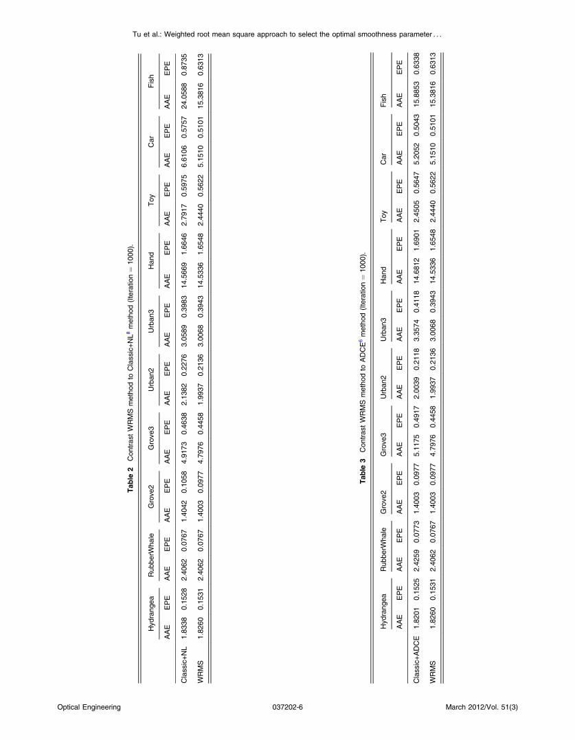
In the second experiment, we check whether our WRMSmethod does automatically determine the optimal smooth-ness parameter λ. We compare the state-of-the-art “Classic+NL” algorithm, which uses the fixed smoothness parameterλ based on experience, with our WRMS method. Table 2shows that our approach outperforms the “Classic+NL”algorithm in most of the examples. For some sequences,like Toy, Car, Fish, we find a surprised improvement. Forthese sequences, the suitable λ value was unknown, sothe “Classic+NL” algorithm, which simply selects the λwithout reference to experience and without setting it toa fixed value, is separated from practice. Instead, ourWRMS method would automatically determine the optimalλ without ground truth and experience.

In the third experiment, we compare the performance ofour WRMS method to automatically determine the optimalsmoothness parameter λ with the state-of-the-art ADCEapproach. The results presented in Table 3 show that ourmethod is superior to the ADCE approach for most of thesequences, except for the high quality ones in which theprimary motion of the objects are constant speed on a lineartrajectory (like Hydrangea). For sequences (like Car, Fish)with a complex background and low resolution, ourWRMS method still outperforms the ADCE approach,even if the objects move with a constant speed along a lineartrajectory.

In these above three experiments, we selected thereference λ0 according to our methodology outlined inSec. 3.1. For the highest quality and resolution sequences,such as RubberWhale, Grove2, Grove3, Hand, Urban3,we set λ0 ¼ 3; For Urban2 and Hydrangea whose qualityis a little lower than Urban3, we set a little higher valueof λ0 ¼ 5. Based on this principle, we used the followingvalues for other sequences: Toy, λ0 ¼ 12; Car, λ0 ¼ 20;Fish, λ0 ¼ 25.

In our last experiment, we investigate three complex realscene sequences from the Middlebury benchmark databasewhich include occlusion, large displacement, small-scalestructures, illumination changes, shadows, etc. (we useframe 9, frame 10, and frame 11 in the three sequences tobe tested). We compare “Classic+NL” and ADCE methodswith our approach to test the practicality and effectiveness ofWRMS. In this test, we set λ0 ¼ 12 for the three sequencesbased on their quality.

Figure 2 shows that, when comparing the color opticalflow field Figs. 2(a), 2(c), and 2(e) of the three methods,our WRMS method represents the complex movements ofthe legs almost completely correct, where the big girl’slegs are nearly totally occluded by the little girl. In Fig. 3,which compares the movement of the small balls inFigs. 3(a), 3(c), and 3(e), we can see that our approach per-forms much better than the other two methods. The warpedframes Figs. 3(b), 3(d), and 3(f) reflect that the “Classic+NL”method and the ADCE method both fail to estimate themotion of the balls because it is hard to handle large displa-cements with small scale structures, as pointed out in

Tab

le1

Con

tras

tWRMS

metho

dto

RMS

metho

d,ce

ntrald

ifferen

ceweigh

tWRS

(WRMS_C

)metho

d(Iteratio

n¼

1000

).

Hyd

rang

eaRub

berW

hale

Grove

2Grove

3Urban

2Urban

3Han

dToy

Car

Fish

AAE

EPE

AAE

EPE

AAE

EPE

AAE

EPE

AAE

EPE

AAE

EPE

AAE

EPE

AAE

EPE

AAE

EPE

AAE

EPE

RMS

1.85

180.15

352.40

620.07

671.47

170.10

424.84

390.45

651.99

480.21

363.30

210.40

6914

.539

01.67

092.49

260.56

655.20

520.50

4315

.885

30.63

38

WRMS_C

1.85

180.15

352.40

620.07

671.41

570.09

774.79

760.44

581.99

480.21

363.07

680.41

4314

.533

61.65

482.49

880.56

695.15

100.51

0115

.392

70.64

42

WRMS

1.82

600.15

312.40

620.07

671.40

030.09

774.79

760.44

581.99

370.21

203.00

680.39

4314

.533

61.65

482.44

400.56

225.15

100.51

0115

.381

60.63

13

Tu et al.: Weighted root mean square approach to select the optimal smoothness parameter : : :

Optical Engineering 037202-5 March 2012/Vol. 51(3)

Tab

le3

Con

tras

tWRMS

metho

dto

ADCE6metho

d(Iteratio

n¼

1000

).

Hyd

rang

eaRub

berW

hale

Grove

2Grove

3Urban

2Urban

3Han

dToy

Car

Fish

AAE

EPE

AAE

EPE

AAE

EPE

AAE

EPE

AAE

EPE

AAE

EPE

AAE

EPE

AAE

EPE

AAE

EPE

AAE

EPE

Class

ic+ADCE

1.82

010.15

252.42

590.07

731.40

030.09

775.11

750.49

172.00

390.21

183.35

740.41

1814

.681

21.69

012.45

050.56

475.20

520.50

4315

.885

30.63

38

WRMS

1.82

600.15

312.40

620.07

671.40

030.09

774.79

760.44

581.99

370.21

363.00

680.39

4314

.533

61.65

482.44

400.56

225.15

100.51

0115

.381

60.63

13

Tab

le2

Con

tras

tWRMS

metho

dto

Class

ic+NL8

metho

d(Iteratio

n¼

1000

).

Hyd

rang

eaRub

berW

hale

Grove

2Grove

3Urban

2Urban

3Han

dToy

Car

Fish

AAE

EPE

AAE

EPE

AAE

EPE

AAE

EPE

AAE

EPE

AAE

EPE

AAE

EPE

AAE

EPE

AAE

EPE

AAE

EPE

Class

ic+NL

1.83

380.15

282.40

620.07

671.40

420.10

584.91

730.46

382.13

820.22

763.05

890.39

8314

.566

91.66

462.79

170.59

756.61

060.57

5724

.058

80.87

35

WRMS

1.82

600.15

312.40

620.07

671.40

030.09

774.79

760.44

581.99

370.21

363.00

680.39

4314

.533

61.65

482.44

400.56

225.15

100.51

0115

.381

60.63

13

Tu et al.: Weighted root mean square approach to select the optimal smoothness parameter : : :

Optical Engineering 037202-6 March 2012/Vol. 51(3)

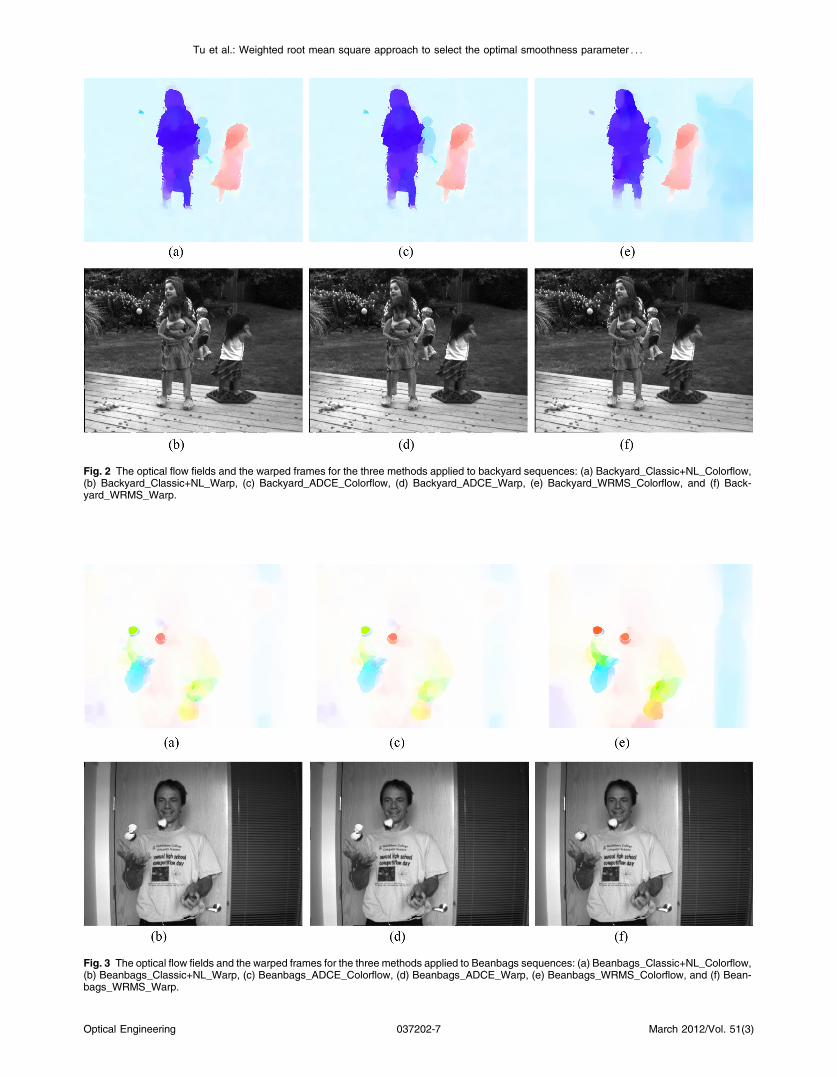
Fig. 2 The optical flow fields and the warped frames for the three methods applied to backyard sequences: (a) Backyard_Classic+NL_Colorflow,(b) Backyard_Classic+NL_Warp, (c) Backyard_ADCE_Colorflow, (d) Backyard_ADCE_Warp, (e) Backyard_WRMS_Colorflow, and (f) Back-yard_WRMS_Warp.

Fig. 3 The optical flow fields and the warped frames for the three methods applied to Beanbags sequences: (a) Beanbags_Classic+NL_Colorflow,(b) Beanbags_Classic+NL_Warp, (c) Beanbags_ADCE_Colorflow, (d) Beanbags_ADCE_Warp, (e) Beanbags_WRMS_Colorflow, and (f) Bean-bags_WRMS_Warp.

Tu et al.: Weighted root mean square approach to select the optimal smoothness parameter : : :

Optical Engineering 037202-7 March 2012/Vol. 51(3)

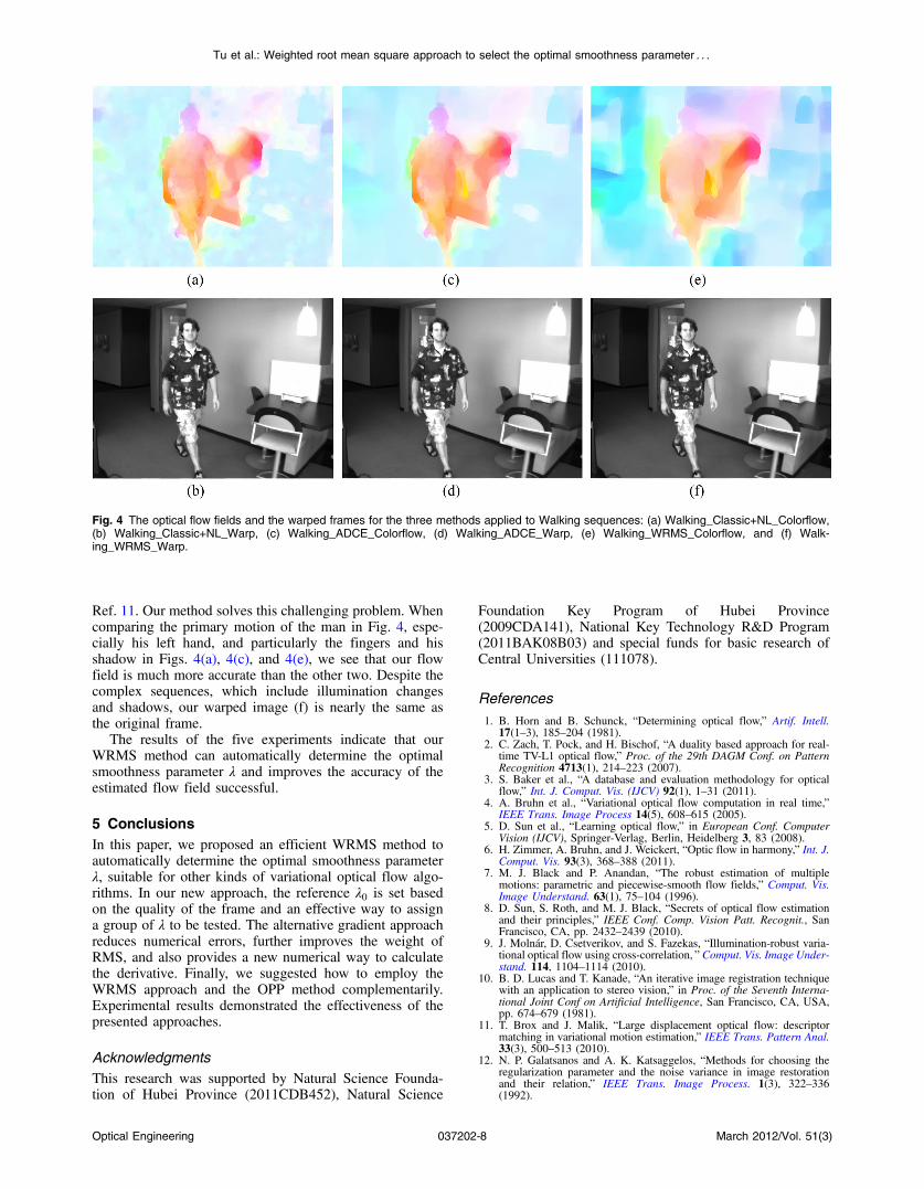
Ref. 11. Our method solves this challenging problem. Whencomparing the primary motion of the man in Fig. 4, espe-cially his left hand, and particularly the fingers and hisshadow in Figs. 4(a), 4(c), and 4(e), we see that our flowfield is much more accurate than the other two. Despite thecomplex sequences, which include illumination changesand shadows, our warped image (f) is nearly the same asthe original frame.

The results of the five experiments indicate that ourWRMS method can automatically determine the optimalsmoothness parameter λ and improves the accuracy of theestimated flow field successful.

5 ConclusionsIn this paper, we proposed an efficient WRMS method toautomatically determine the optimal smoothness parameterλ, suitable for other kinds of variational optical flow algo-rithms. In our new approach, the reference λ0 is set basedon the quality of the frame and an effective way to assigna group of λ to be tested. The alternative gradient approachreduces numerical errors, further improves the weight ofRMS, and also provides a new numerical way to calculatethe derivative. Finally, we suggested how to employ theWRMS approach and the OPP method complementarily.Experimental results demonstrated the effectiveness of thepresented approaches.

AcknowledgmentsThis research was supported by Natural Science Founda-tion of Hubei Province (2011CDB452), Natural Science

Foundation Key Program of Hubei Province(2009CDA141), National Key Technology R&D Program(2011BAK08B03) and special funds for basic research ofCentral Universities (111078).

References

1. B. Horn and B. Schunck, “Determining optical flow,” Artif. Intell.17(1–3), 185–204 (1981).

2. C. Zach, T. Pock, and H. Bischof, “A duality based approach for real-time TV-L1 optical flow,” Proc. of the 29th DAGM Conf. on PatternRecognition 4713(1), 214–223 (2007).

3. S. Baker et al., “A database and evaluation methodology for opticalflow,” Int. J. Comput. Vis. (IJCV) 92(1), 1–31 (2011).

4. A. Bruhn et al., “Variational optical flow computation in real time,”IEEE Trans. Image Process 14(5), 608–615 (2005).

5. D. Sun et al., “Learning optical flow,” in European Conf. ComputerVision (IJCV), Springer-Verlag, Berlin, Heidelberg 3, 83 (2008).

6. H. Zimmer, A. Bruhn, and J. Weickert, “Optic flow in harmony,” Int. J.Comput. Vis. 93(3), 368–388 (2011).

7. M. J. Black and P. Anandan, “The robust estimation of multiplemotions: parametric and piecewise-smooth flow fields,” Comput. Vis.Image Understand. 63(1), 75–104 (1996).

8. D. Sun, S. Roth, and M. J. Black, “Secrets of optical flow estimationand their principles,” IEEE Conf. Comp. Vision Patt. Recognit., SanFrancisco, CA, pp. 2432–2439 (2010).

9. J. Molnár, D. Csetverikov, and S. Fazekas, “Illumination-robust varia-tional optical flow using cross-correlation, ” Comput. Vis. Image Under-stand. 114, 1104–1114 (2010).

10. B. D. Lucas and T. Kanade, “An iterative image registration techniquewith an application to stereo vision,” in Proc. of the Seventh Interna-tional Joint Conf on Artificial Intelligence, San Francisco, CA, USA,pp. 674–679 (1981).

11. T. Brox and J. Malik, “Large displacement optical flow: descriptormatching in variational motion estimation,” IEEE Trans. Pattern Anal.33(3), 500–513 (2010).

12. N. P. Galatsanos and A. K. Katsaggelos, “Methods for choosing theregularization parameter and the noise variance in image restorationand their relation,” IEEE Trans. Image Process. 1(3), 322–336(1992).

Fig. 4 The optical flow fields and the warped frames for the three methods applied to Walking sequences: (a) Walking_Classic+NL_Colorflow,(b) Walking_Classic+NL_Warp, (c) Walking_ADCE_Colorflow, (d) Walking_ADCE_Warp, (e) Walking_WRMS_Colorflow, and (f) Walk-ing_WRMS_Warp.

Tu et al.: Weighted root mean square approach to select the optimal smoothness parameter : : :

Optical Engineering 037202-8 March 2012/Vol. 51(3)

13. L. Ng and V. Solo, “A data-driven method for choosing smoothingparameters in optical flow problems,” in IEEE International Conf.on Image Processing, Santa Barbara, CA, pp. 360–363 (1997).

14. K. Krajsek and R. Mester, “Bayesian model selection for optical flowestimation,” Pattern Recogn. 4713, 142–151 (2007).

15. S. Baker and I. Matthews, “Lucas-Kanade 20 years on: a unifyingframework,” Int. J. Comput. Vis. 56(3), 221–225 (2004).

16. L. I. Rudin, S. Osher, and E. Fatemi, “Nonlinear total variation basednoise removal algorithms,” Phys. Nonlinear Phenom. 60(1–4), 259–268(1992).

17. P. Sand and S. Teller, “Particle video: long-range motion estimationusing point trajectories,” Int. J. Comput. Vis. 80(1), 72–91 (2008).

18. T. Ishikawa, I. Matthews, and S. Baker, “Efficient image alignment withoutlier rejection,” in: Technique Report CMU-RI-TR-02-27, RoboticsInstitute, Carnegie Mellon University (October 2002).

19. C. Liu et al.“Human-assisted motion annotation,” IEEE Conf. on Com-puter Vision and Pattern Recognition (CVPR), Anchorage, AK, pp. 1–8(2008) http://people.csail.mit.edu/celiu/motionAnnotation/.

Zhigang Tu started his MPhil PhD in imageprocessing in the School of Electronic Infor-mation, Wuhan University, China, 2008.Since September 2011, he has been withthe Multimedia and Geometry Group atUtrecht University, Netherlands. His Currentresearch interests include optical flowestimation, super-resolution construction,multimedia systems and technologies,human-computer interaction, and mobilecomputing.

Wei Xie received his BE degree in electronicinformation engineering and PhD degree incommunication and information systemfrom Wuhan University, China, in 2004 and2010, respectively. He currently works atComputer School of Wuhan University,China. His research interests include super-resolution reconstruction, image fusion andimage quality assessment.

Wolfgang Hürst is an assistant professorat the Department of Information and Com-puting Sciences at Utrecht University,Netherlands. His research interests includemultimedia systems and technologies,human-computer interaction, mobile comput-ing. Hürst has a PhD in computer sciencefrom the University of Freiburg, Germany,and a Masters in computer science fromthe University of Karlsruhe, Germany. FromJanuary 1996 to March 1997, he was a visit-

ing researcher at Carnegie Mellon University in Pittsburgh, USA.From March 2005 through October 2007, he worked as researchassociate at the University of Freiburg, Germany.

Shufen Xiong is a graduate student inSchool of Electronic Information at WuhanUniversity, China. Her research interestsare motion estimation and segmentation incomputer vision.

Qianqing Qin received the PhD Degree inScience at NanKaiUniversity, China, in1989. He held position of Assistant Professorin Huazhong University of Science and Tech-nology from 1991 to 1995. Since 1995, hebecame a full professor at Ocean Universityof China. From 1999 through the present, hehas been a professor in Wuhan University,China. His research interests include imageprocessing, computer vision, and Waveletcomputing.

Tu et al.: Weighted root mean square approach to select the optimal smoothness parameter : : :

Optical Engineering 037202-9 March 2012/Vol. 51(3)