1

Weighted Graphs

CB

A

E

D

F

0

328

5 8

48

7 1

2 5

2

3 9

2

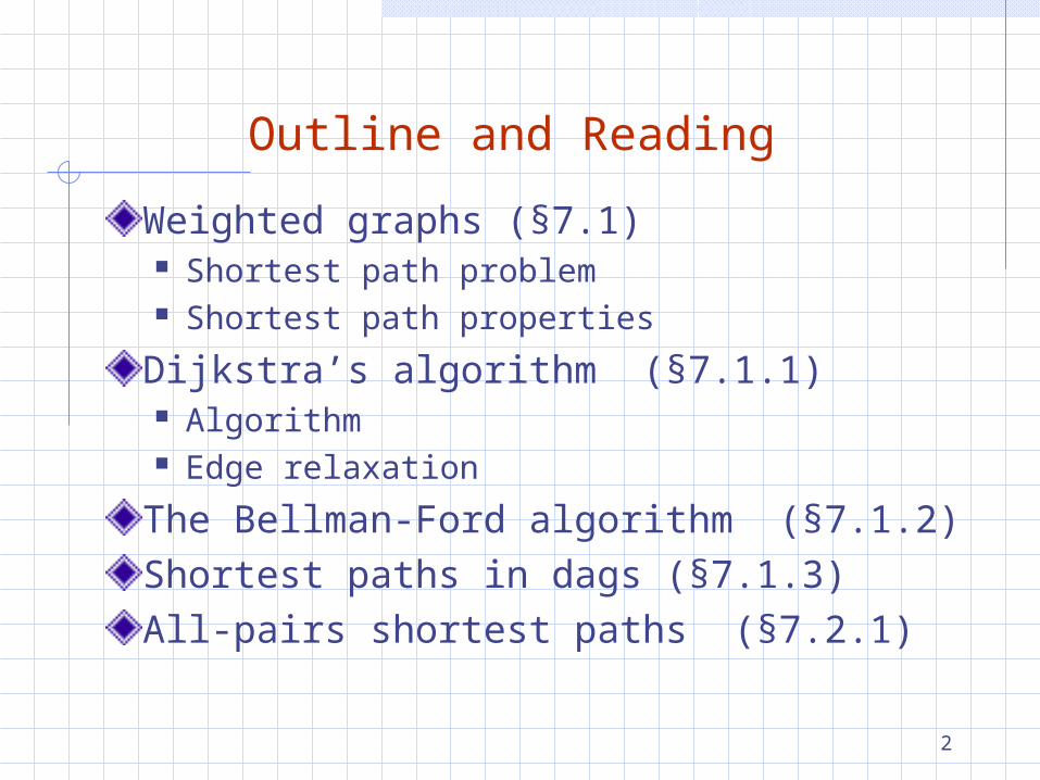
Outline and Reading

Weighted graphs (§7.1) Shortest path problem Shortest path properties

Dijkstra’s algorithm (§7.1.1) Algorithm Edge relaxation

The Bellman-Ford algorithm (§7.1.2)Shortest paths in dags (§7.1.3)All-pairs shortest paths (§7.2.1)

3

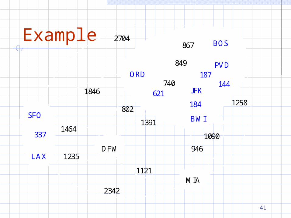
Weighted GraphsIn a weighted graph, each edge has an associated numerical value, called the weight of the edgeEdge weights may represent, distances, costs, etc.Example: In a flight route graph, the weight of an edge

represents the distance in miles between the endpoint airports

ORD PVD

MIADFW

SFO

LAX

LGA

HNL

849

802

13871743

1843

10991120

1233337

2555

142

12

05

4

Shortest Path ProblemGiven a weighted graph and two vertices u and v, we want to find a path of minimum total weight between u and v. Length of a path is the sum of the weights of its edges.

Example: Shortest path between Providence and Honolulu

Applications Internet packet routing Flight reservations Driving directions

ORD PVD

MIADFW

SFO

LAX

LGA

HNL

849

802

13871743

1843

10991120

1233337

2555

142

12

05

5

Shortest Path PropertiesProperty 1:

A subpath of a shortest path is itself a shortest pathProperty 2:

There is a tree of shortest paths from a start vertex to all the other vertices

Example:Tree of shortest paths from Providence

ORD PVD

MIADFW

SFO

LAX

LGA

HNL

849

802

13871743

1843

10991120

1233337

2555

142

12

05

6

Dijkstra’s Algorithm

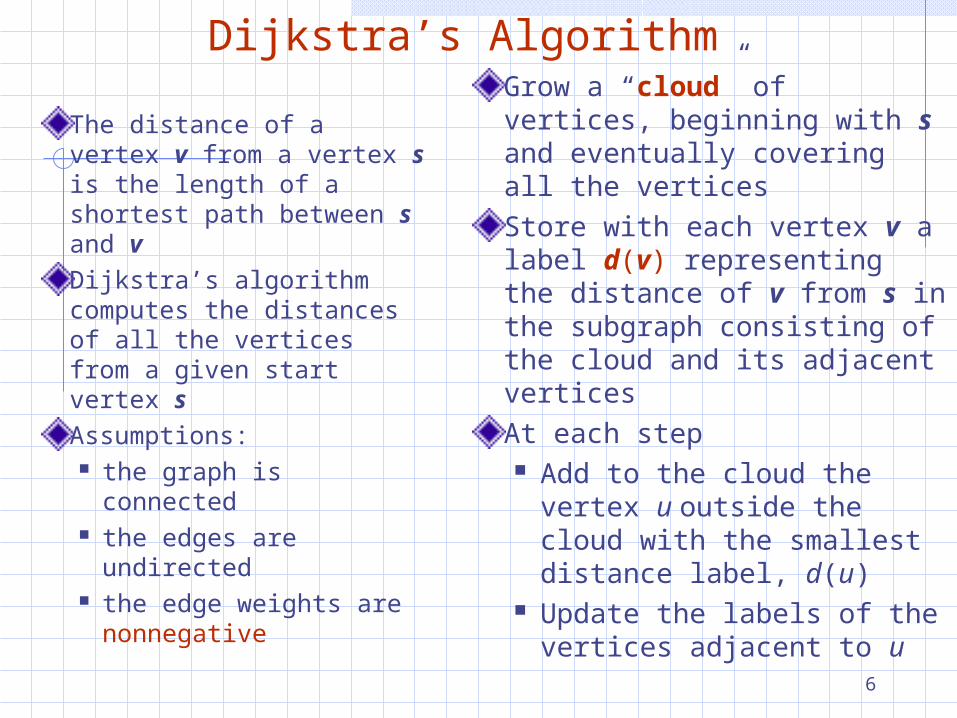
The distance of a vertex v from a vertex s is the length of a shortest path between s and vDijkstra’s algorithm computes the distances of all the vertices from a given start vertex sAssumptions: the graph is

connected the edges are

undirected the edge weights are

nonnegative

Grow a “cloud” of vertices, beginning with s and eventually covering all the verticesStore with each vertex v a label d(v) representing the distance of v from s in the subgraph consisting of the cloud and its adjacent verticesAt each step Add to the cloud the vertex

u outside the cloud with the smallest distance label, d(u)

Update the labels of the vertices adjacent to u

7

Edge RelaxationConsider an edge e (u,z) such that u is the vertex

most recently added to the cloud

z is not in the cloud

The relaxation of edge e updates distance d(z) as follows:d(z) min{d(z),d(u) weight(e)}

d(z) 75

d(u) 5010

zsu

d(z) 60

d(u) 5010

zsu

e

e

8

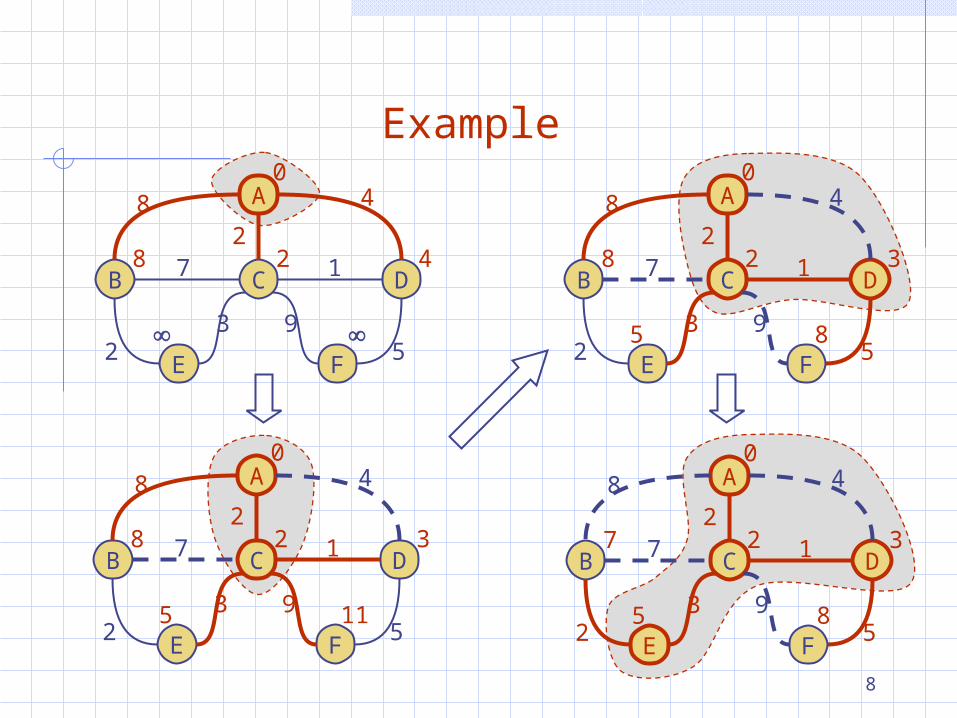
Example

CB

A

E

D

F

0

428

48

7 1

2 5

2

3 9

CB

A

E

D

F

0

328

5 11

48

7 1

2 5

2

3 9

CB

A

E

D

F

0

328

5 8

48

7 1

2 5

2

3 9

CB

A

E

D

F

0

327

5 8

48

7 1

2 5

2

3 9

9

Example (cont.)

CB

A

E

D

F

0

327

5 8

48

7 1

2 5

2

3 9

CB

A

E

D

F

0

327

5 8

48

7 1

2 5

2

3 9

10

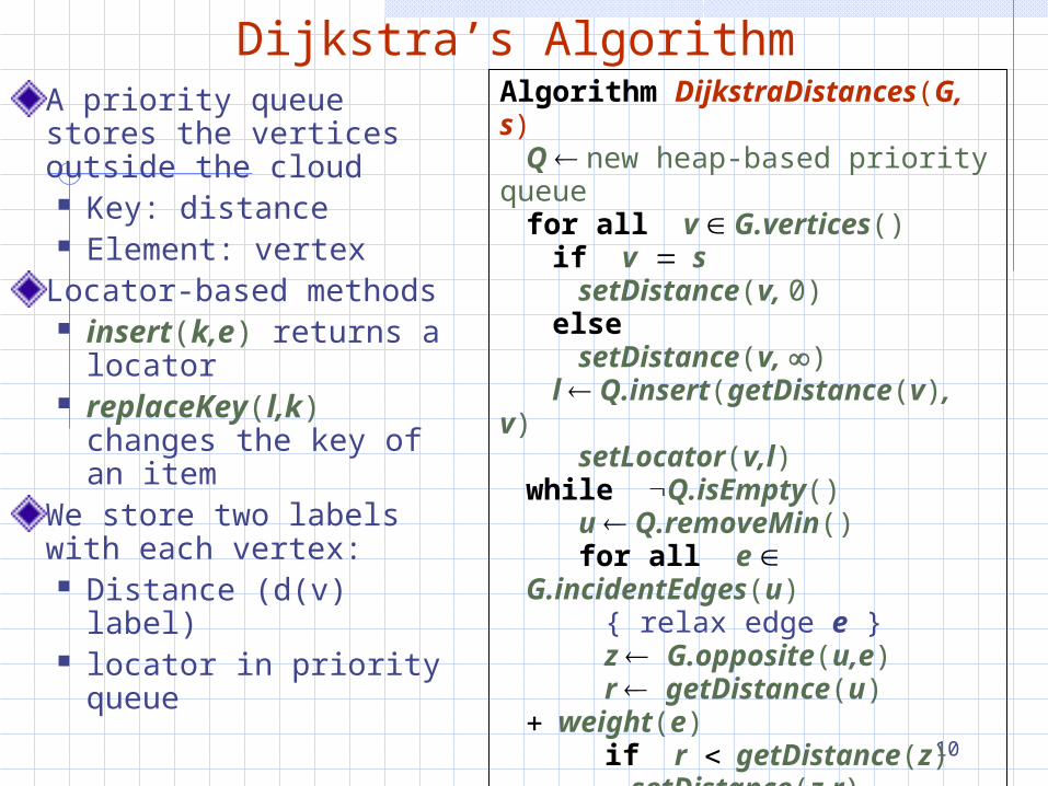
Dijkstra’s AlgorithmA priority queue stores the vertices outside the cloud Key: distance Element: vertex

Locator-based methods insert(k,e) returns a

locator replaceKey(l,k)

changes the key of an item

We store two labels with each vertex: Distance (d(v) label) locator in priority

queue

Algorithm DijkstraDistances(G, s)Q new heap-based priority queuefor all v G.vertices()

if v ssetDistance(v, 0)

else setDistance(v, )

l Q.insert(getDistance(v), v)setLocator(v,l)

while Q.isEmpty()u Q.removeMin() for all e G.incidentEdges(u)

{ relax edge e }z G.opposite(u,e)r getDistance(u) weight(e)if r getDistance(z)

setDistance(z,r) Q.replaceKey(getLocator(z),r)

11

AnalysisGraph operations Method incidentEdges is called once for each vertex

Label operations We set/get the distance and locator labels of vertex

z O(deg(z)) times Setting/getting a label takes O(1) time

Priority queue operations Each vertex is inserted once into and removed once

from the priority queue, where each insertion or removal takes O(log n) time

The key of a vertex in the priority queue is modified at most deg(w) times, where each key change takes O(log n) time

12

Dijkstra’s Algorithm

Dijkstra’s algorithm runs in O((n m) log n) time provided the graph is represented by the adjacency list structure Recall that v deg(v) 2m

The running time can also be expressed as O(m log n) since the graph is connected

13

ExtensionUsing the template method pattern, we can extend Dijkstra’s algorithm to return a tree of shortest paths from the start vertex to all other verticesWe store with each vertex a third label: parent edge in the

shortest path treeIn the edge relaxation step, we update the parent label

Algorithm DijkstraShortestPathsTree(G, s

…for all v G.vertices()

…setParent(v, )

…for all e G.incidentEdges(u)

{ relax edge e }z G.opposite(u,e)r getDistance(u)

weight(e)if r getDistance(z)

setDistance(z,r)setParent(z,e)

Q.replaceKey(getLocator(z),r)

14

Why Dijkstra’s Algorithm Works

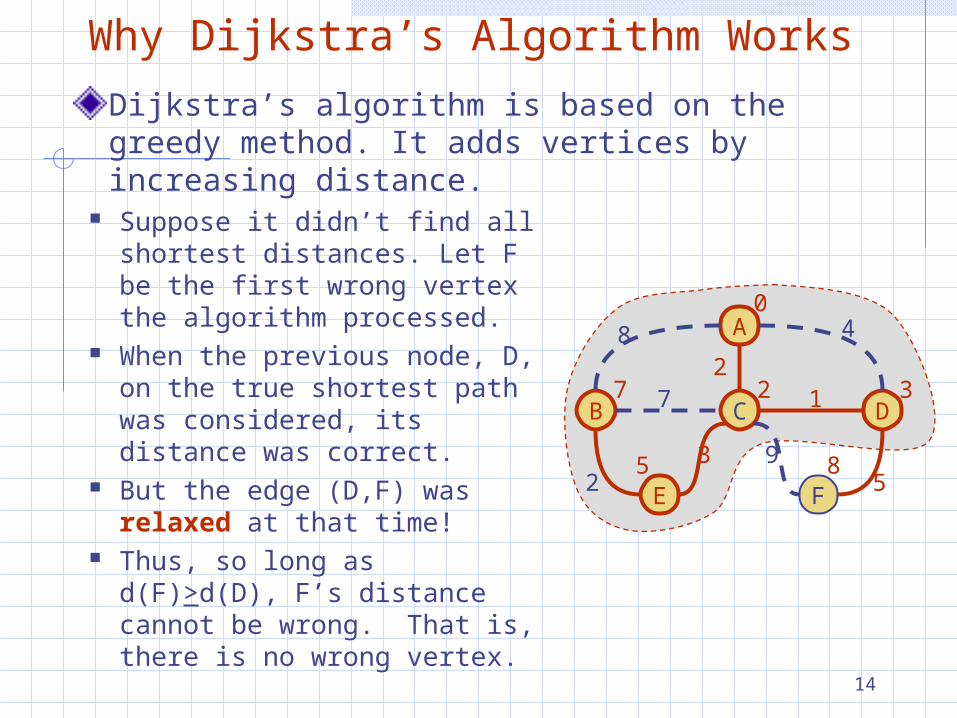
Dijkstra’s algorithm is based on the greedy method. It adds vertices by increasing distance.

CB

A

E

D

F

0

327

5 8

48

7 1

2 5

2

3 9

Suppose it didn’t find all shortest distances. Let F be the first wrong vertex the algorithm processed.

When the previous node, D, on the true shortest path was considered, its distance was correct.

But the edge (D,F) was relaxed at that time!

Thus, so long as d(F)>d(D), F’s distance cannot be wrong. That is, there is no wrong vertex.

15

Why It Doesn’t Work for Negative-Weight Edges

If a node with a negative incident edge were to be added late to the cloud, it could mess up distances for vertices already in the cloud.

CB

A

E

D

F

0

457

5 9

48

7 1

2 5

6

0 -8

Dijkstra’s algorithm is based on the greedy method. It adds vertices by increasing distance.

C’s true distance is 1, but it is already in the cloud with

d(C)=5!

16

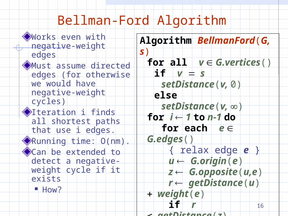
Bellman-Ford AlgorithmWorks even with negative-weight edgesMust assume directed edges (for otherwise we would have negative-weight cycles)Iteration i finds all shortest paths that use i edges.Running time: O(nm).Can be extended to detect a negative-weight cycle if it exists How?

Algorithm BellmanFord(G, s)for all v G.vertices()

if v ssetDistance(v, 0)

else setDistance(v, )

for i 1 to n-1 dofor each e G.edges()

{ relax edge e }u G.origin(e)z G.opposite(u,e)r getDistance(u)

weight(e)if r getDistance(z)

setDistance(z,r)

17

-2

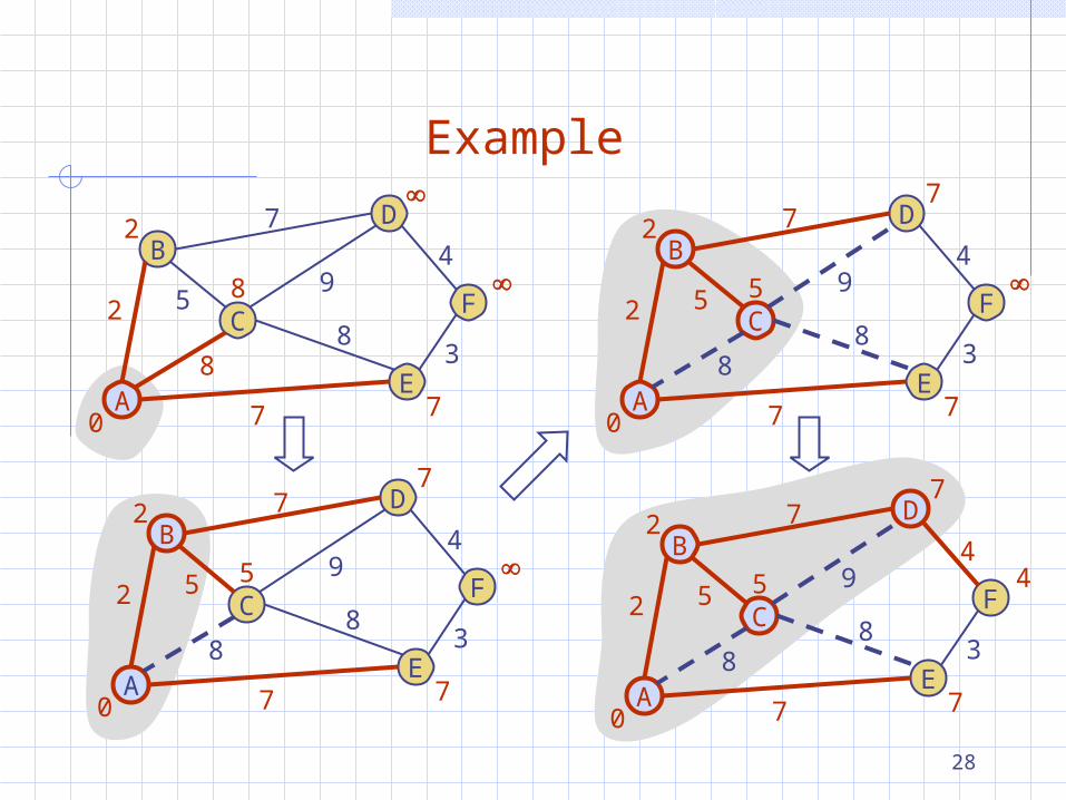
Bellman-Ford Example

0

48

7 1

-2 5

-2

3 9

0

48

7 1

-2 53 9

Nodes are labeled with their d(v) values. At the end of the algorithm each d(v) is shortest distance from the 0 node to v.

-2

-28

0

4

48

7 1

-2 53 9

8 -2 4

-15

61

9

-25

0

1

-1

9

48

7 1

-2 5

-2

3 94

18

DAG-based AlgorithmWorks even with negative-weight edgesUses topological orderDoesn’t use any fancy data structuresIs much faster than Dijkstra’s algorithmRunning time: O(n+m).

Algorithm DagDistances(G, s)for all v G.vertices()

if v ssetDistance(v, 0)

else setDistance(v, )

Perform a topological sort of the vertices

for u 1 to n do {in topological order}

for each e G.outEdges(u){ relax edge e }z G.opposite(u,e)r getDistance(u)

weight(e)if r getDistance(z)

setDistance(z,r)

19

-2

DAG Example

0

48

7 1

-5 5

-2

3 9

0

48

7 1

-5 53 9

Nodes are labeled with their d(v) values

-2

-28

0

4

48

7 1

-5 53 9

-2 4

-1

1 7

-25

0

1

-1

7

48

7 1

-5 5

-2

3 94

1

1

2 43

6 5

1

2 43

6 5

8

1

2 43

6 5

1

2 43

6 5

5

0

(two steps)

20

All-Pairs Shortest PathsFind the distance between every pair of vertices in a weighted directed graph G.We can make n calls to Dijkstra’s algorithm (if no negative edges), which takes O(nmlog n) time.Likewise, n calls to Bellman-Ford would take O(n2m) time.We can achieve O(n3) time using dynamic programming (similar to the Floyd-Warshall algorithm).

Algorithm AllPair(G) {assumes vertices 1,…,n} for all vertex pairs (i,j)

if i jD0[i,i] 0

else if (i,j) is an edge in GD0[i,j] weight of edge (i,j)

elseD0[i,j] +

for k 1 to n do for i 1 to n do for j 1 to n do

Dk[i,j] min{Dk-1[i,j], Dk-1[i,k]+Dk-

1[k,j]} return Dn

k

j

i

Uses only verticesnumbered 1,…,k-1 Uses only vertices

numbered 1,…,k-1

Uses only vertices numbered 1,…,k(compute weight of this edge)

21

Minimum Spanning Trees

JFK

BOS

MIA

ORD

LAXDFW

SFO BWI

PVD

8672704

187

1258

849

144740

1391

184

946

1090

1121

2342

1846 621

802

1464

1235

337

22

Outline and Reading

Minimum Spanning Trees (§7.3) Definitions A crucial fact

The Prim-Jarnik Algorithm (§7.3.2)

Kruskal's Algorithm (§7.3.1)

Baruvka's Algorithm (§7.3.3)

23

Minimum Spanning TreeSpanning subgraph

Subgraph of a graph G containing all the vertices of G

Spanning tree Spanning subgraph that is

itself a (free) treeMinimum spanning tree (MST)

Spanning tree of a weighted graph with minimum total edge weight

Applications Communications networks Transportation networks

ORD

PIT

ATL

STL

DEN

DFW

DCA

101

9

8

6

3

25

7

4

24

Cycle Property

Cycle Property: Let T be a minimum

spanning tree of a weighted graph G

Let e be an edge of G that is not in T and let C be the cycle formed by e with T

For every edge f of C, weight(f) weight(e)

Proof: By contradiction If weight(f) weight(e) we

can get a spanning tree of smaller weight by replacing e with f

84

2 36

7

7

9

8e

C

f

84

2 36

7

7

9

8

C

e

f

Replacing f with e yieldsa better spanning tree

25

U V

Partition PropertyPartition Property:

Consider a partition of the vertices of G into subsets U and V

Let e be an edge of minimum weight across the partition

There is a minimum spanning tree of G containing edge e

Proof: Let T be an MST of G If T does not contain e, consider

the cycle C formed by e with T and let f be an edge of C across the partition

By the cycle property,weight(f) weight(e)

Thus, weight(f) weight(e) We obtain another MST by

replacing f with e

74

2 85

7

3

9

8 e

f

74

2 85

7

3

9

8 e

f

Replacing f with e yieldsanother MST

U V

26

Prim-Jarnik’s AlgorithmSimilar to Dijkstra’s algorithm (for a connected graph)We pick an arbitrary vertex s and we grow the MST as a cloud of vertices, starting from sWe store with each vertex v a label d(v) = the smallest weight of an edge connecting v to a vertex in the cloud

At each step: We add to the cloud the vertex u outside the cloud with the smallest distance label We update the labels of the vertices adjacent to u

27

Prim-Jarnik’s Algorithm (cont.)A priority queue stores the vertices outside the cloud Key: distance Element: vertex

Locator-based methods insert(k,e) returns a

locator replaceKey(l,k) changes

the key of an itemWe store three labels with each vertex: Distance Parent edge in MST Locator in priority

queue

Algorithm PrimJarnikMST(G)Q new heap-based priority queues a vertex of Gfor all v G.vertices()

if v ssetDistance(v, 0)

else setDistance(v, )

setParent(v, )l Q.insert(getDistance(v), v)

setLocator(v,l)while Q.isEmpty()

u Q.removeMin() for all e

G.incidentEdges(u)z G.opposite(u,e)r weight(e)if r getDistance(z)

setDistance(z,r)setParent(z,e)

Q.replaceKey(getLocator(z),r)

28

Example

BD

C

A

F

E

74

28

5

7

3

9

8

07

2

8

BD

C

A

F

E

74

28

5

7

3

9

8

07

2

5

7

BD

C

A

F

E

74

28

5

7

3

9

8

07

2

5

7

BD

C

A

F

E

74

28

5

7

3

9

8

07

2

5 4

7

29

Example (contd.)

BD

C

A

F

E

74

28

5

7

3

9

8

03

2

5 4

7

BD

C

A

F

E

74

28

5

7

3

9

8

03

2

5 4

7

30

AnalysisGraph operations Method incidentEdges is called once for each vertex

Label operations We set/get the distance, parent and locator labels of

vertex z O(deg(z)) times Setting/getting a label takes O(1) time

Priority queue operations Each vertex is inserted once into and removed once

from the priority queue, where each insertion or removal takes O(log n) time

The key of a vertex w in the priority queue is modified at most deg(w) times, where each key change takes O(log n) time

31

Analysis

Prim-Jarnik’s algorithm runs in O((n m) log n) time provided the graph is represented by the adjacency list structure Recall that v deg(v) 2m

The running time is O(m log n) since the graph is connected

32

Kruskal’s AlgorithmA priority queue stores the edges outside the cloud Key: weight Element: edge

At the end of the algorithm We are left with

one cloud that encompasses the MST

A tree T which is our MST

Algorithm KruskalMST(G)for each vertex V in G do

define a Cloud(v) of {v}let Q be a priority queue.Insert all edges into Q using

their weights as the keyT while T has fewer than n-1

edges do edge e = T.removeMin()

Let u, v be the endpoints of e

if Cloud(v) Cloud(u) then

Add edge e to TMerge Cloud(v) and

Cloud(u)return T

33

Data Structure for Kruskal AlgortihmThe algorithm maintains a forest of treesAn edge is accepted it if connects distinct treesWe need a data structure that maintains a partition, i.e., a collection of disjoint sets, with the operations:

-find(u): return the set storing u -union(u,v): replace the sets storing u and v

with their union

34

Representation of a Partition

Each set is stored in a sequenceEach element has a reference back to the set

operation find(u) takes O(1) time, and returns the set of which u is a member.

in operation union(u,v), we move the elements of the smaller set to the sequence of the larger set and update their references

the time for operation union(u,v) is min(nu,nv), where nu and nv are the sizes of the sets storing u and v

Whenever an element is processed, it goes into a set of size at least double, hence each element is processed at most log n times

35

Partition-Based ImplementationA partition-based version of Kruskal’s Algorithm performs cloud merges as unions and tests as finds.Algorithm Kruskal(G):

Input: A weighted graph G.

Output: An MST T for G.

Let P be a partition of the vertices of G, where each vertex forms a separate set.

Let Q be a priority queue storing the edges of G, sorted by their weights

Let T be an initially-empty tree

while Q is not empty do

(u,v) Q.removeMinElement()

if P.find(u) != P.find(v) then

Add (u,v) to T

P.union(u,v)

return T

Running time: O((n+m)log n)

36

Kruskal Example

JFK

BOS

MIA

ORD

LAXDFW

SFO BWI

PVD

8672704

187

1258

849

144740

1391

184

946

1090

1121

2342

1846 621

802

1464

1235

337

37

JFK

BOS

MIA

ORD

LAXDFW

SFO BWI

PVD

8672704

187

1258

849

144740

1391

184

946

1090

1121

2342

1846 621

802

1464

1235

337

Example

38

Example

JFK

BOS

MIA

ORD

LAXDFW

SFO BWI

PVD

8672704

187

1258

849

144740

1391

184

946

1090

1121

2342

1846 621

802

1464

1235

337

39

Example

JFK

BOS

MIA

ORD

LAXDFW

SFO BWI

PVD

8672704

187

1258

849

144740

1391

184

946

1090

1121

2342

1846 621

802

1464

1235

337

40

Example

JFK

BOS

MIA

ORD

LAXDFW

SFO BWI

PVD

8672704

187

1258

849

144740

1391

184

946

1090

1121

2342

1846 621

802

1464

1235

337

41

Example

JFK

BOS

MIA

ORD

LAXDFW

SFO BWI

PVD

8672704

187

1258

849

144740

1391

184

946

1090

1121

2342

1846 621

802

1464

1235

337

42

Example

JFK

BOS

MIA

ORD

LAXDFW

SFO BWI

PVD

8672704

187

1258

849

144740

1391

184

946

1090

1121

2342

1846 621

802

1464

1235

337

43

Example

JFK

BOS

MIA

ORD

LAXDFW

SFO BWI

PVD

8672704

187

1258

849

144740

1391

184

946

1090

1121

2342

1846 621

802

1464

1235

337

44

Example

JFK

BOS

MIA

ORD

LAXDFW

SFO BWI

PVD

8672704

187

1258

849

144740

1391

184

946

1090

1121

2342

1846 621

802

1464

1235

337

45

Example

JFK

BOS

MIA

ORD

LAXDFW

SFO BWI

PVD

8672704

187

1258

849

144740

1391

184

946

1090

1121

2342

1846 621

802

1464

1235

337

46

Example

JFK

BOS

MIA

ORD

LAXDFW

SFO BWI

PVD

8672704

187

1258

849

144740

1391

184

946

1090

1121

2342

1846 621

802

1464

1235

337

47

Example

JFK

BOS

MIA

ORD

LAXDFW

SFO BWI

PVD

8672704

187

1258

849

144740

1391

184

946

1090

1121

2342

1846 621

802

1464

1235

337

48

Example

JFK

BOS

MIA

ORD

LAXDFW

SFO BWI

PVD

8672704

187

1258

849

144740

1391

184

946

1090

1121

2342

1846 621

802

1464

1235

337

49

Example

JFK

BOS

MIA

ORD

LAXDFW

SFO BWI

PVD

8672704

187

1258

849

144740

1391

184

946

1090

1121

2342

1846 621

802

1464

1235

337

50

Baruvka’s Algorithm

Like Kruskal’s Algorithm, Baruvka’s algorithm grows many “clouds” at once.

Each iteration of the while-loop halves the number of connected compontents in T. The running time is O(m log n).

Algorithm BaruvkaMST(G)T V {just the vertices of G}

while T has fewer than n-1 edges dofor each connected component C in T do

Let edge e be the smallest-weight edge from C to another component in T.

if e is not already in T thenAdd edge e to T

return T

51

JFK

BOS

MIA

ORD

LAXDFW

SFO BWI

PVD

8672704

187

1258

849

144740

1391

184

946

1090

1121

2342

1846621

802

1464

1235

337

Baruvka Example

52

Example

JFK

BOS

MIA

ORD

LAXDFW

SFO BWI

PVD

8672704

187

1258

849

144740

1391

184

946

1090

1121

2342

1846621

802

1464

1235

337

53

Example

JFK

BOS

MIA

ORD

LAXDFW

SFO BWI

PVD

8672704

187

1258

849

144740

1391

184

946

1090

1121

2342

1846621

802

1464

1235

337