Weighted Averages on Surfaces

Daniele Panozzo1 Ilya Baran2,3,4 Olga Diamanti1 Olga Sorkine-Hornung1

1ETH Zurich 2Belmont Technology, Inc. 3Adobe Research 4Disney Research, Zurich

Figure 1: Interactive control for various geometry processing and modeling applications made possible with weighted averages on surfaces.From left to right: texture transfer, decal placement, semiregular remeshing and Laplacian smoothing, splines on surfaces.

Abstract

We consider the problem of generalizing affine combinations in Eu-clidean spaces to triangle meshes: computing weighted averages ofpoints on surfaces. We address both the forward problem, namelycomputing an average of given anchor points on the mesh withgiven weights, and the inverse problem, which is computing theweights given anchor points and a target point. Solving the forwardproblem on a mesh enables applications such as splines on surfaces,Laplacian smoothing and remeshing. Combining the forward andinverse problems allows us to define a correspondence mapping be-tween two different meshes based on provided corresponding pointpairs, enabling texture transfer, compatible remeshing, morphingand more. Our algorithm solves a single instance of a forward oran inverse problem in a few microseconds. We demonstrate thatanchor points in the above applications can be added/removed andmoved around on the meshes at interactive framerates, giving theuser an immediate result as feedback.

Keywords: surface geometry, weighted averages, correspondence

Links: DL PDF WEB VIDEO

1 Introduction

Computing weighted averages, or affine combinations of points inEuclidean space is a fundamental operation. Given n anchor pointsand corresponding weights, their weighted average can be easilycomputed by coordinate-wise weighted averaging. In this paper,we explore a generalization of weighted averages to points on tri-angulated surfaces (meshes) and develop a fast method for find-ing them. The natural way to generalize weighted averages to anarbitrary metric space is the Frechet mean [Cartan 1929; Frechet

1948]: it is defined as the point that minimizes the sum of weightedsquared distances to the anchors. How to find this point, however,is not obvious from the definition, and this task has so far receivedlittle attention in the literature.

The Frechet mean is typically studied with Riemannian metrics,such as geodesic distance. Computing geodesic distance betweentwo arbitrary points on a triangle mesh, even despite the latest ad-vancements, is relatively expensive. We therefore focus on a dif-ferent class of metrics, which we call Euclidean-embedding met-rics, that are derived by embedding the mesh in a (possibly high-dimensional) Euclidean space and computing Euclidean distancein that space. A number of known metrics, such as diffusion dis-tance, commute-time distance and biharmonic distance [Lipmanet al. 2010] are Euclidean-embedding metrics. We adapt the con-struction of Rustamov and colleagues [2009] to obtain a Euclidean-embedding metric that mimics geodesic distance.

We show that for a Euclidean-embedding metric, the Frechet meantakes a special form: it is the result of taking the Euclidean weightedaverage of the points in the embedding space and projecting it (i.e.,finding the closest point) onto the embedded mesh. However, theembedded mesh is not a smooth surface, and the Euclidean projec-tion operator exhibits discontinuities near mesh edges. The Frechetmean therefore also behaves discontinuously. We introduce a newprojection operator which can be seen as a generalization of Phongprojection [Kobbelt et al. 1999] to Euclidean spaces of dimensionhigher than three, and use this operator instead of the Euclideanprojection. We show experimentally that our Phong projection be-haves in a qualitatively similar way to Euclidean projection onto asmooth surface, although no smooth surface is actually constructed.

Armed with this Phong projection operator, we develop fast algo-rithms for computing the forward problem and the inverse problem.The forward problem is to find the weighted average of several an-chors, given the anchors and the weights. The inverse problem is tocompute weights for a given set of anchors, such that the weightedaverage is a given target point. In the Euclidean space, the inverseproblem is known as generalized barycentric coordinates. Unlikethe forward problem, the inverse problem has been previously stud-ied from a computational point of view for geodesic distances [Rus-tamov 2010], and we give a solution for our setup.

Weighted averages are a fundamental building block that can beused for a variety of tasks in computer graphics and geometric mod-eling. Using the forward problem, we construct splines on meshes

and remesh surfaces semiregularly. Using both the forward andthe inverse problem together allows us to define a dense correspon-dence between two meshes, which we can use to transfer surface-varying data, such as a texture, from one mesh to another or set upa morph between them. While all of the above tasks have special-ized higher-quality algorithms, our methods are several orders ofmagnitude faster. We can perform all mentioned tasks interactively,providing more feedback to the user, and setting a new point on theperformance-vs-quality tradeoff curve.

Our main technical contributions are:1. We develop Phong projection in higher dimensions as a

smoother alternative to Euclidean projection.2. We present new generalized barycentric coordinates for scat-

tered points.3. We present an efficient algorithm for solving the forward

problem.

2 Related work

The mathematical basis for weighted averages in a general metricspace is the Frechet mean [Cartan 1929; Frechet 1948], also knownas the Karcher mean [Karcher 1977] and the Riemannian center ofmass. It is typically used with geodesic distance or other Rieman-nian metrics. However, geodesic distance is not C1 and is sensitiveto noise on meshes (Figure 10). Moreover, computing the geodesicdistance is relatively costly [Surazhsky et al. 2005], since it needsto be done exactly (small errors in the distance can change the min-imum location unpredictably), and between arbitrary points on themesh (not just vertices). This may preclude recent fast approximatemethods [Sethian 1996; Xin et al. 2012; Crane et al. 2013]. In-stead, we use a metric obtained by embedding the mesh in a high-dimensional Euclidean space, which is smooth and very fast to eval-uate.

Methods for computing the Frechet mean have been developedon spheres [Buss and Fillmore 2001] and rotation groups [Pen-nec 1998]. Methods for computing other kinds of weighted aver-ages have been proposed for different subgroups of matrices [Alexa2002; Palfia 2009]. Somewhat surprisingly, to the best of ourknowledge, no efficient algorithms for computing the Frechet meanhave been previously presented for general surfaces.

For the inverse problem, there generally exists more than one setof weights for which given anchors average to a given point. Formost applications, however, a particular weight vector is needed.Weights that vary smoothly and have other desirable properties areknown as generalized barycentric coordinates. Their constructionis a well-studied problem in Euclidean space [Floater 2003; Juet al. 2005; Joshi et al. 2007; Lipman et al. 2007]. Langer andcolleagues [2006] define generalized barycentric coordinates on asphere and Rustamov [2010] on arbitrary surfaces as we do. How-ever, the generalized barycentric coordinate schemes that Rustamovuses are defined for polygons, while we have a set of anchors in noparticular order. We therefore use a simple scheme generalizing arecent idea by Waldron [2011] and Moving Least Squares (MLS).MLS interpolation has been generalized to surfaces [Jin et al. 2009]using geodesic distance, which has to be recomputed whenever ananchor changes. Rustamov’s method suffers from the same draw-back.

Prior methods have used interpolated tangent planes and normalsat vertices to obtain smoother behavior on triangle meshes in 3D.The classical example of such a method is Phong shading [Phong1975]. Kobbelt and colleagues [1999] use projection along thePhong normal to construct multiresolution mesh hierarchies. Reg-istration techniques [Chen and Medioni 1991] and other methods

[Sander et al. 2000] establish correspondences between nearby sur-faces by shooting rays in the interpolated normal direction fromone surface to the other. Phong tessellation [Boubekeur and Alexa2008] uses tangent planes at mesh vertices to replace triangles withquadratic patches for smoother display. We develop an analog ofPhong projection [Kobbelt et al. 1999] in higher dimensions forour purposes (Section 3.2).

Since weighted averages can be used for a variety of tasks, webriefly review the relevant literature for the most important appli-cations of our framework.

Cross-parametrization. Recently, a lot of effort has been spenton establishing mappings between surfaces, due to the large num-ber of practical applications that benefit from it, such as texturetransfer and morphing [Eckstein et al. 2001; Tzur and Tal 2009].The computed map may be optimized to be as isometric as possi-ble [Ovsjanikov et al. 2010] or as conformal as possible [Kim et al.2011]. In [Schreiner et al. 2004], progressive meshes are used tofind the mapping, while in [Kraevoy and Sheffer 2004] the meshesare simplified and parametrized on a common base domain. Othersimilar methods have been developed [Sumner and Popovic 2004;Yeh et al. 2011]. None of these techniques are fast enough to beinteractive. Our method, while not specialized for this task, can beused to define a cross-parametrization between two surfaces givencompatible anchors. When the anchors are changed (i.e., removed,added or displaced), our map can be updated at interactive rates,whereas all prior methods require minutes of computation or moreon complicated cases.

On-surface deformations. Weighted averages on surfaces cansimilarly be used to construct a mapping from a surface to itself andthus deform a signal defined on it. An alternative method tailoredto this problem was presented by Ritschel and colleagues [2010],who show various applications of on-surface deformations, allow-ing artists to control shadows, caustics and deform textures interac-tively. They simulate a piece of elastic cloth sliding over the surfaceand use a specialized GPU solver to achieve interactive frame rates.Constrained parametrization [Hormann et al. 2008] could also beused for the same goal, but handling surfaces with genus greaterthan one is complicated and computationally expensive.

Splines on surfaces. Buss and Fillmore [2001] demonstratedspherical splines as an application of their averaging operator.Spline curves on general surfaces have been studied in a varia-tional setting [Hofer and Pottmann 2004], but the necessary op-timization is relatively costly. Jin and colleagues [2009] definedcurves on surfaces as iso-contours of an interpolated scalar field,but again, the computational requirements are significant. Wallnerand Pottmann [2006] introduced an averaging-based definition ofsplines over smooth surfaces, where an averaging operator that pro-duces points on the surface is defined. Their approach is to simplycompute the weighted average in 3D space and project the resultonto the surface. This is similar to our method, but without a high-dimensional embedding and without Phong projection the resultscan be less robust (Figure 3, left) and discontinuous on discretemeshes.

3 Method

Our method consists of several building blocks. We startby introducing notation and terminology for the Frechet meanand Euclidean-embedding metrics and establishing some basicfacts (Section 3.1). We then introduce Phong projection for higherdimensions (Section 3.2), describe our method for computing theforward problem (Section 3.3), and then show how to solve the in-verse problem of generalized barycentric coordinates (Section 3.4).

Finally we describe how we construct the specific Euclidean-embedding metric that we use (Section 3.5).

3.1 Preliminaries

We refer to the n points xi whose average is to be computed as an-chors. In Rk, the forward problem is solved simply by coordinate-wise averaging using the given weights wi,

Pwi = 1:

x =

nX

i=1

wixi. (1)

The generalization of weighted averages to metric spaces is calledthe Frechet mean. The Frechet mean of n anchors and weights wi

over a metric space M with metric d is defined as:

x = argminx2M

F (x), where F (x) =

nX

i=1

wi d(x,xi)2

. (2)

As long as d is smooth, the gradient of F (x) at the minimum x

must be zero:nX

i=1

wi rd(x,xi)2 = 0. (3)

For Euclidean space, rd(x,xi)2 = x� xi and it is easy to check

that the Frechet mean definition reduces to the usual one (1).

In general, the Frechet mean is not always well-defined: F (x) mayhave multiple minima. For example, on a sphere, consider anchorsthat are vertices of a platonic solid, and identical weights. If d is theEuclidean metric of the ambient 3D space then F is constant, and ifd is the geodesic metric on the sphere then F has multiple minimadue to symmetry. Even if F has a unique minimum, its locationmay not be continuous in wi and xi, and Equation (3) can be satis-fied at a local minimum. Karcher [1977] and Kendall [1990] amongothers have studied the conditions for which the Frechet mean iswell-behaved on Riemannian manifolds. At a high-level, if the an-chors are close together, Gaussian curvature is not too high, andthe weights are nonnegative, x is well-defined and continuous inall variables. Our focus is on fast computation, and we leave it upto the user to ensure that there are enough close-by anchors; ourexperiments show that this is not difficult (see the accompanyingvideo for an example of anchor placement).

While the Frechet mean is usually used with geodesic distances,geodesics between arbitrary points on a mesh are slow to compute.

Figure 2: Cubic B-splines on surfaces are shown as yellow curves.The red curve is a linear spline and illustrates the control polygon.

Euclidean Phong Euclidean Phong

Figure 3: Left: A line segment in 3D space projected onto a meshusing Euclidean and Phong projection. Right: Quad remeshing(see Section 4) using Euclidean and Phong projection in RD . No-tice the jagginess of the Euclidean projections.

A different class of metrics, that we call Euclidean-embedding met-rics, has been gaining popularity in recent literature. A Euclidean-embedding metric is defined by an embedding e : M ! RD andthe distance between two points on the surface is the Euclidean dis-tance between their embeddings d(x

1

,x

2

) = ke(x1

)�e(x2

)k. Ona mesh, the embedding is defined on the vertices and is linear overeach face interior. Euclidean-embedding metrics are very fast toevaluate, and if e is smooth, there is no C1-discontinuous cut locus,unlike with geodesic distance. In this work, we always computedistances using a Euclidean embedding; see Section 3.5 for detailson how this embedding is constructed.

For a Euclidean-embedding metric, the Frechet mean has a sim-pler form. Letting yi = e(xi) and substituting the metric into thedefinition of F , we obtain:

F (x) =

nX

i=1

wike(x)� yik2. (4)

Letting y =Pn

i=1

wiyi and using thatP

wi = 1, we can simplifyF to:

F (x) =

nX

i=1

⇣wi e(x)

Te(x)� 2wi e(x)

Tyi + wi y

Ti yi

⌘=

= e(x)T e(x)� 2 e(x)T y +

nX

i=1

wi yTi yi =

= ke(x)� yk2 � y

Ty +

nX

i=1

wi yTi yi, (5)

where only the first term depends on x. Thus, we have just shownthat minimizing F over the original surface in R3 is equivalent tominimizing the distance to y, the weighted average of the anchorsin the embedding spaceRD . The computation of the Frechet meanfor a Euclidean-embedding metric thus consists of computing theEuclidean weighted average y in the embedding space and project-ing it onto the embedded mesh. Because a mesh is not smooth,Euclidean projection, and therefore the exact Frechet mean, is nota smooth function of the weights or the anchor locations. Wetherefore use a different projection operator that provides a better-behaved weighted average.

Smooth projection. The Euclidean projection operator y =PE(y) that projects y onto a mesh M is discontinuous at the me-dial axis of the mesh. Because, unlike for smooth surfaces, themedial axis of a mesh extends all the way to the mesh edges, theprojection operator is discontinuous no matter how close y is to themesh. Even away from the medial axis, PE has undesirable behav-ior, as shown in Figure 3.

Assuming that the mesh is approximating a smooth surface, onewould like a projection operator with smoother behavior. Onecan use the fact that projection onto a smooth surface is alwaysalong the direction perpendicular to the surface. Kobbelt and col-leagues [1999] propose projecting along a continuous normal fieldin 3D, as follows (see also [Botsch and Sorkine 2008] , SectionIID): If y is a projection of y, and n is the normal at y, thenn ⇥ (y � y) = 0. For a mesh embedded in 3D one can takeestimated surface normals at the mesh vertices and define a contin-uous surface normal on the mesh triangles using barycentric inter-polation (as is commonly done for Phong shading). This simulatesthe behavior of projecting onto a smooth surface without actuallyhaving a smooth surface. Suppose that at vertex i of a triangle t

(for i = 1, 2, 3) the vertex position is vi and the normal is ni. Toproject y, [Kobbelt et al. 1999] look for a point y on the trianglet with barycentric coordinates ⇠i that satisfy:

(⇠1

n

1

+ ⇠

2

n

2

+ ⇠

3

n

3

)⇥ (⇠1

v

1

+ ⇠

2

v

2

+ ⇠

3

v

3

� y) = 0. (6)

For a mesh embedded in D-dimensional space, the normal is not avector, but a (D � 2)-dimensional subspace, hence the above con-struction does not directly generalize. To make Phong projectionwork for a D-dimensional space, we use the fact that the normalat y is the subspace orthogonal to the tangent plane at y, and so asimilar construction can be developed by interpolating the tangentplanes at the triangle’s vertices instead of normals. Note that it issimilar, but not equivalent to the previous one in 3D, since linearlyinterpolating bases of tangent planes is different than interpolatingthe normals. Interpolating bases can, however, be more easily ex-tended to work in higher dimensional spaces. Since the same tan-gent plane can be represented by an infinite number of bases, wemust carefully select which basis we use for the linear interpolationto avoid degeneracies. The next section describes our Phong pro-jection more formally; the supplemental material provides a moreextended description.

3.2 Phong projection

We denote our triangle mesh as M = (V, E ,F) with embed-ded vertices V ⇢ RD . Each vertex has an associated tangentplane (computed e.g. using the Loop [1987] limit stencil inRD), represented by two basis vectors, which we assume tobe orthonormal. Denote the tangent planes at the verticesof a triangle t = (v

1

,v

2

,v

3

) as T

1

, T

2

, T

3

2 R2⇥D . Let (⇠

1

, ⇠

2

, ⇠

3

) 2 R2⇥D be an interpolated tangent plane basis forthe point ⇠

1

v

1

+ ⇠

2

v

2

+ ⇠

3

v

3

inside t, where ⇠i are barycentriccoordinates. will be precisely defined later (Definition 3).

Definition 1. A point y = ⇠

1

v

1

+ ⇠

2

v

2

+ ⇠

3

v

3

on the triangle t

having vertices vi is a Phong projection of y 2 RD onto t if:

(⇠1

, ⇠

2

, ⇠

3

)(⇠1

v

1

+ ⇠

2

v

2

+ ⇠

3

v

3

� y) = 0, (7)⇠

1

+ ⇠

2

+ ⇠

3

= 1, (8)⇠i � 0. (9)

As previously discussed, a Phong projection is a point y on thetriangle, where the interpolated tangent plane is perpendicularto the line connecting y and y. Note that this characterizationcorresponds to the Euclidean projection onto a smooth manifold.

Definition 2. The Phong projection of a point y onto a mesh M isthe closest Phong projection with respect to every triangle of M.

Unlike Euclidean projection, the Phong projection onto a trianglemay not exist or multiple points on a single triangle may be Phong

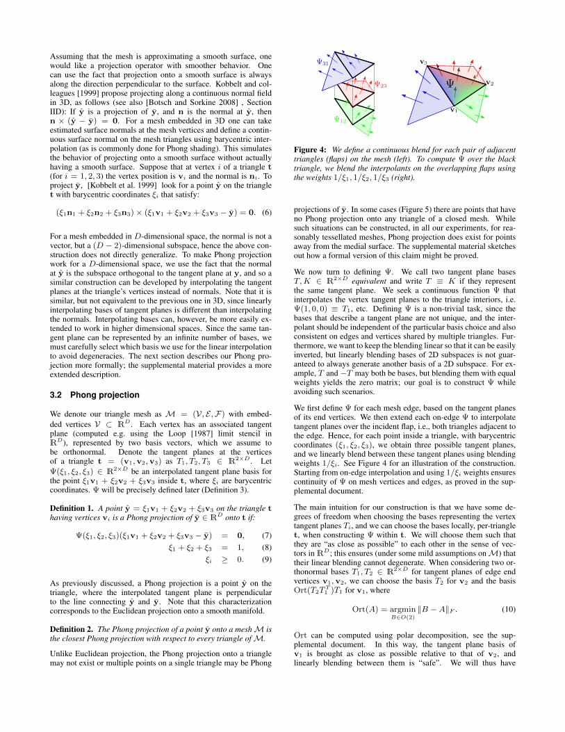
�31

�23 �

v1

v2

v3

�12

Figure 4: We define a continuous blend for each pair of adjacenttriangles (flaps) on the mesh (left). To compute over the blacktriangle, we blend the interpolants on the overlapping flaps usingthe weights 1/⇠

1

, 1/⇠2

, 1/⇠3

(right).

projections of y. In some cases (Figure 5) there are points that haveno Phong projection onto any triangle of a closed mesh. Whilesuch situations can be constructed, in all our experiments, for rea-sonably tessellated meshes, Phong projection does exist for pointsaway from the medial surface. The supplemental material sketchesout how a formal version of this claim might be proved.

We now turn to defining . We call two tangent plane basesT,K 2 R2⇥D equivalent and write T ⌘ K if they representthe same tangent plane. We seek a continuous function thatinterpolates the vertex tangent planes to the triangle interiors, i.e. (1, 0, 0) ⌘ T

1

, etc. Defining is a non-trivial task, since thebases that describe a tangent plane are not unique, and the inter-polant should be independent of the particular basis choice and alsoconsistent on edges and vertices shared by multiple triangles. Fur-thermore, we want to keep the blending linear so that it can be easilyinverted, but linearly blending bases of 2D subspaces is not guar-anteed to always generate another basis of a 2D subspace. For ex-ample, T and �T may both be bases, but blending them with equalweights yields the zero matrix; our goal is to construct whileavoiding such scenarios.

We first define for each mesh edge, based on the tangent planesof its end vertices. We then extend each on-edge to interpolatetangent planes over the incident flap, i.e., both triangles adjacent tothe edge. Hence, for each point inside a triangle, with barycentriccoordinates (⇠

1

, ⇠

2

, ⇠

3

), we obtain three possible tangent planes,and we linearly blend between these tangent planes using blendingweights 1/⇠i. See Figure 4 for an illustration of the construction.Starting from on-edge interpolation and using 1/⇠i weights ensurescontinuity of on mesh vertices and edges, as proved in the sup-plemental document.

The main intuition for our construction is that we have some de-grees of freedom when choosing the bases representing the vertextangent planes Ti, and we can choose the bases locally, per-trianglet, when constructing within t. We will choose them such thatthey are “as close as possible” to each other in the sense of vec-tors inRD; this ensures (under some mild assumptions on M) thattheir linear blending cannot degenerate. When considering two or-thonormal bases T

1

, T

2

2 R2⇥D for tangent planes of edge endvertices v

1

,v

2

, we can choose the basis T

2

for v2

and the basisOrt(T

2

T

T1

)T1

for v1

, where

Ort(A) = argminB2O(2)

kB �AkF . (10)

Ort can be computed using polar decomposition, see the sup-plemental document. In this way, the tangent plane basis ofv

1

is brought as close as possible relative to that of v

2

, andlinearly blending between them is “safe”. We will thus have

Figure 5: In some cases, Phong projection may not exist. On theleft, we discretize a circle as a hexagon with exact normals. Thepoints in each colored region project to the corresponding edge. Onthe right, we slightly rotate all the normals clockwise. The whitehexagon in the middle now consists of points that do not have aPhong projection.

12

(⇠1

, ⇠

2

, 0) ⌘ ⇠

1

R

12

T

1

+ ⇠

2

T

2

, where R12

= Ort(T2

T

T1

), andsimilarly

23

, 31

for the other edges of a triangle t.

We have an additional degree of freedom to exploit: the tangentplane bases at v

1

,v

2

can both be rotated in-plane by the same 2⇥2orthogonal matrix E

12

without changing the planes themselvesand without affecting their linear blending, up to equivalence(and the same holds for the other edges). We choose the matricesE

12

, E

23

, E

31

such that the bases we linearly blend in the end foreach point inside t are as close as possible to each other. Formally:

Definition 3. Tangent plane interpolation:

(⇠1

, ⇠

2

, ⇠

3

) =⇠

1

⇠

2

⇠

3

⇠

1

⇠

2

+ ⇠

2

⇠

3

+ ⇠

3

⇠

1

✓1

⇠

3

12

(⇠1

, ⇠

2

, ⇠

3

)+ (11)

+1

⇠

1

23

(⇠1

, ⇠

2

, ⇠

3

) +1

⇠

2

31

(⇠1

, ⇠

2

, ⇠

3

)

◆,

where

12

(⇠1

, ⇠

2

, ⇠

3

) = ⇠

1

E

12

R

12

T

1

+⇠

2

E

12

T

2

+⇠

3

1

2(E

23

+E

31

R

31

)T3

.

The formulas for the other edge blends 23

, 31

are obtained bycyclic permutation of the indices. Eij 2 R2⇥2 are computed as

E

12

, E

23

, E

31

= argminE12,E23,E312O(2)

X

1i<j6

kAi �Ajk2F , (12)

where A

1

= E

12

R

12

T

1

, A

2

= E

12

T

2

, A

3

= E

23

R

23

T

2

,A

4

= E

23

T

3

, A5

= E

31

R

31

T

3

, A6

= E

31

T

1

. The E matri-ces can be iteratively optimized by fixing two out of the three andsolving a Procrustes problem for the third, which is guaranteed todecrease the energy; this optimization converges quickly. We referto the supplemental for a more detailed explanation of the construc-tion of and for a formal proof of its continuity and interpolationproperties.

Phong projection has several useful properties:1. Phong projection takes each point on the mesh to itself.

Proof. When y is on the mesh and ⇠

1

, ⇠2

, ⇠3

are its barycen-tric coordinates, Equation (7) is trivially satisfied.

2. Phong projection onto a plane is the same as Euclidean pro-jection.Proof. For a discretized plane, all tangent planes and triangleplanes are the same. will be constant and identical to them:the resulting projection will thus simply be the Euclidean pro-jection onto the triangle.

(a) Eucl. projection onto (b) Phong projection (c) Euclidean projectiona smooth surface onto a mesh onto a mesh

Figure 6: Comparison of the qualitative behavior of (a) projectiononto a smooth surface, (b) Phong projection, and (c) Euclideanprojection onto a mesh. The smooth surface is a torus, which isdiscretized in (b) and (c). Each image shows a plane through thecenter of the torus; each point is colored based on the angle be-tween the vector from that point to its projection and the x-axis.Phong projection behaves similarly to projecting onto the smoothtorus, while Euclidean projection shows clear discontinuities.

3. If the Euclidean projection of a point y onto a tangent planeat vertex v is v itself, then v is a Phong projection of y.Proof. Assume w.l.o.g. that v is the first vertex in the triangle.Then (1, 0, 0) is by definition the tangent plane at v, andEquation 7 corresponds to Euclidean projection.

4. Assume that a point y, which is on an edge shared by trianglest

1

and t

2

, is a Phong projection of a point y onto t

1

. Then y

is also a Phong projection of y onto t

2

.Proof. Equation (7) is identical in both triangles up to an in-dex permutation, and is the same due to continuity.

5. Given a point y on a triangle, the set of points in ambientspace for which y is a Phong projection is an affine subspace.Proof. Equation (7) is linear in y, so its solution set is anaffine subspace.

The third and fourth properties explain why Phong projection isconsistent on mesh vertices and edges, and are the reasons for ourinvolved definition, and the fifth property allows us to solve theinverse problem with relative ease.

Phong projection on a triangle is computed by solving Equations (7)and (8), using Newton’s method starting from ( 1

3

,

1

3

,

1

3

); the solu-tion is discarded if Equation (9) is not satisfied.

We illustrate the advantage of Phong projection in Figures 3 and 6.

3.3 The forward problem

To compute the weighted average of n anchors over a Euclidean-embedding metric, we first use the embedding to map them to RD

and compute their weighted average y in Euclidean space. Theremaining task is then to find the Phong projection of y onto theembedded mesh. The simplest brute-force approach is to computethe Phong projection onto every triangle and pick the closest point,but this is very expensive. Acceleration structures, such as KD-trees or bounding volume hierarchies are typically used to speed upEuclidean projection, but they scale poorly to higher dimensions.

Instead, we use a simple local search approach, based on the factthat Euclidean and Phong projections are fairly close. We start withan initial guess vertex, for example, the vertex closest to the pro-jection from a previous computation, or the anchor with the highestweight, if a better initial guess is not available. We then walk overthe edge graph, greedily choosing edges that get us closer to y,

Figure 7: Example of remeshing using weighted averages. From left to right: the original mesh, a coarse quad mesh, a uniformly subdividedquad mesh (without Laplacian smoothing), and the final result after 5 steps of Laplacian smoothing on the surface.

stopping when we hit a vertex closer to y than all of its neighbors.From that vertex, we do a breadth-first search over triangles, tryingto find a Phong projection on each triangle and stopping as soon aswe find a triangle for which a Phong projection exists.

This method is not guaranteed to find the Phong projection, but itfails when there are multiple close projection candidates and theweighted average is therefore meaningless. We compared the re-sults of this method to the brute force solution for all of the forwardproblems in Figure 7 and the projections are all exactly the same.For the forward problems in Figure 12, the covering by anchors isnot perfect and our method produced different results on 2.5 percentof the pixels, with a maximum error of 7 times the average lengthof a mesh edge.

3.4 The inverse problem

For many applications, we need to be able to compute, for givenanchors and a given point on the surface x, a set of weights w =(w

1

, . . . , wn)T for which x is the weighted average (the weights

must sum to one). In Euclidean space, finding such weights isknown as the generalized barycentric coordinates problem. Rusta-mov [2010] solves this problem for the Frechet mean with geodesicdistances, but we need to be able to invert our formulation to beconsistent with the forward problem.

There are many ways to define the generalized barycentric coordi-nates, since Equation (3) has multiple solutions. The particular so-lution needs to satisfy three properties: locality, interpolation, andsmoothness. Locality means that the anchors that are far away fromx should have very low weights. This is important for most appli-cations shown in Section 4 because it restricts the effect of everyanchor to a small region around it. Interpolation means that whenx coincides with an anchor, the weight for all other anchors shouldbe zero. Finally smoothness means that small changes to anchorsand x result in small changes to the weights. Many existing gen-eralized barycentric coordinates satisfy these properties, but theyassume that the anchors are given as a simple polygon. For our ap-plications we cannot use such schemes because the polygon wouldhave to change its connectivity in order to remain simple as the an-chors move, violating smoothness.

Instead, we propose a new set of generalized barycentric coordi-nates, obtained by simply treating the Phong projection and parti-tion of unity as linear constraints and solving a quadratic optimiza-tion problem that penalizes weights for far-away anchors. Given apoint on a triangle t with barycentric coordinates ⇠, we solve:

arg minw

kDwk2 (13)

s.t. (⇠1

, ⇠

2

, ⇠

3

)(⇠1

v

1

+ ⇠

2

v

2

+ ⇠

3

v

3

�X

i

wiyi) = 0,

X

i

wi = 1.

D is a diagonal matrix that contains a weighting term for every an-chor. This is a standard linearly-constrained minimum-norm prob-lem, which we solve using the pseudoinverse.

We are left with the problem of defining D. Note that for far-awayanchors whose weights should be low, Di,i should be high. Addi-tionally, we penalize anchors far away from the tangent plane morebecause they are likely to be less reliable. Given the locations (inthe embedded mesh) of the anchors, yi = e(xi), and of the in-put surface point, y = e(x), we split the vector yi � y into thecomponent vT in the tangent plane at y and the component vO or-thogonal to the tangent plane. Using Di,i = kvT k2 + �kvOk2guarantees interpolation: if a given point on the surface is also ananchor i, then Di,i = 0 and the weight combination that assignswi = 1 and wj = 0 for all other anchors satisfies the constraintsand sets the objective in (13) to zero; the quadratic nature of theoptimization problem guarantees uniqueness of this solution. Wehave found that this definition of D works well for a wide range of� (we use 10 for all examples).

This formulation is a weighted variant of Waldron’s method [2011],which, without D, produces weights that are not interpolatory.If one removes the Phong projection constraints, our weights re-duce to Moving Least Squares (see the supplemental material forthe derivation). Our weights are C1 on a smooth manifold, sincethe corresponding MLS formulation generates C1 weights and weare only adding additional linear constraints (on piecewise-linearmeshes the weights are, of course, C0 on the mesh edges).

Maximum Entropy Coordinates [Hormann and Sukumar 2008] sat-isfy all our desiderata, if the inverse of the squared distances is usedas a prior. They lead to similar results to our weights, but are too ex-pensive to compute for our purposes, since they require minimizinga nonlinear energy with Newton’s method.

The accompanying video shows examples of our weights on a sur-face.

3.5 Euclidean-embedding metric

We now discuss how we construct a Euclidean-embedding metricsuitable for our purposes. Lipman et al. [2010] compare several al-ternative metrics: diffusion distance, commute-time distance, andtheir proposed biharmonic distance. These metrics are defined interms of eigenvectors of the Laplace-Beltrami operator, which canbehave poorly, as small features can collapse in the embedding(Figure 8). Instead, we use a metric that is based on Rustamovand colleagues’ [2009] boundary embedding construction.

Rustamov et al. [2009] embed a mesh by computing the geodesicdistances between all pairs of points and using Metric Multidimen-sional Scaling (MMDS) [Cox and Cox 2000] . This approachdoes not scale, as constructing and working with the distance ma-trix for a mesh with 100,000 vertices is impractical: even storingsuch a matrix would require just under 20 GB in single precision.

Euclidean Biharmonic OurEm

bedd

ing

Splines

Figure 8: Top: The original surface (Euclidean embedding) andthe first three dimensions of the biharmonic embedding and ourembedding for the hand mesh. The biharmonic embedding tendsto collapse thin features, making it unsuitable for weighted aver-ages computations on these regions. Bottom: Cubic B-splines us-ing different Euclidean-embedding metrics. Discontinuities in theweighted averages computed with Euclidean and Biharmonic em-beddings can be seen as both the yellow curve passing through thesurface (to connect to a far-away point) and as artifacts on the fin-gers. All of these results were computed using Phong projection.

The IsoCharts method [Zhou et al. 2004] employs Landmark MDS[de Silva and Tenenbaum 2002] to efficiently compute a Euclideanembedding into higher dimensions for spectral mesh segmentationand parameterization applications. We take a conceptually similarlandmark approach and adapt it to our purposes to ensure a smoothembedding. We sample a representative subset S of the mesh ver-tices, compute approximate pairwise geodesic distances only forthese vertices and embed S into RD using MMDS. We then useleast-squares meshes [Sorkine and Cohen-Or 2004] to embed theremaining mesh vertices, creating a mesh in RD whose trianglesare shaped similarly to the original mesh.

We find the subset of mesh vertices S by decimating the mesh usingan algorithm from OpenMesh [Botsch et al. 2002] that iterativelycollapses the halfedge that changes the face normals least. Thisway, the subsequent LS-mesh upsampling will have an easier timecorrectly approximating areas with low curvature. When a user-specified number of points (we use 1000) is left, the decimationstops and these vertices are used as S.

To embed the samples S, we use the fast marching method [Sethian1996] to construct the dissimilarity matrix Q: Qi,j = d

geo

(si, sj) .We use the implementation of MMDS in MATLAB 11, minimizingthe following stress criterion:

nX

i=1

nX

j=1

✓1� ke(si)� e(sj)k

Qi,j

◆2

, (14)

where e(si) 2 RD is the embedding of si. We use D=8 for allexamples. We have not observed any improvement in quality aboveeight dimensions, and as 8 floats fit into an AVX register, we wouldgain little performance improvement from using fewer dimensions.

Denote the set of all original mesh vertices by V = {v1

, . . . , vN},and the final embedded version of each vi by vi 2 RD . To com-plete the embedding v 2 RN⇥D of the remaining vertices V\S,

Euclidean Exact Geodesic

Biharmonic Our metric

Figure 9: Distance and isolines from a point on the tip of the indexfinger using different metrics. Due to the collapse shown in Fig. 8,the isolines of biharmonic distance are aligned with the fingers anddo not discriminate between different points around each finger.

we compute a smooth mesh in the D-dimensional space as a least-squares mesh:

v = argminv

tr⇣v

T �LM

�1

L

�v

⌘

s.t. vi = e(si), 8i 2 S,(15)

where L and M are the stiffness matrix (cotangent Laplacian) andthe lumped mass matrix of the original mesh, respectively [Botschand Sorkine 2008]. The optimization in (15) amounts to solving asparse linear system and we use MATLAB’s built-in solver.

We compare our metric with Euclidean, biharmonic and exactgeodesic distance [Surazhsky et al. 2005] in Figure 9. Our metricis smooth everywhere, while still providing a good approximationof geodesic distance. In Figure 8, we show results of splines de-fined using our algorithm with three different metrics. The overallprecomputation usually takes a few minutes (Table 1).

4 Results

Our method was timed on a quad core 2.6 GHz Intel Core i7 pro-cessor, using all four cores to solve weighted averages problems inparallel. The software is written in C++, manually optimized usingAVX intrinsics and OpenMP, and compiled using the Intel Com-piler. The GPU was only used for rendering and did not participatein timings. Table 1 shows the timings for forward and inverse prob-lems on our meshes. The inverse problem timings appear sublinearin the number of anchors due to a constant time component for con-structing the constraint matrix and solving. The performance of theforward problem is more complicated, depending on mesh structureand anchor placement more than on vertex count.

Below we present some of the possible applications of weightedaverages on surfaces.

4.1 Forward problem

The following applications only make use of the forward problem.

Splines on surfaces. Most splines can be defined in terms ofweighted averages: for example, a point on a B-spline is theweighted average of control points using the basis functions as

Mesh Faces Anchors Forw. Inverse Pre.

pig 8016 27 0.69 µs 0.87 µs 1.1 m3Holes 28800 64 0.64 µs 1.26 µs 1.2 mlizard 39036 93 0.85 µs 1.53 µs 1.9 mchubby 40808 93 0.85 µs 1.57 µs 2.0 mdog 50528 93 1.54 µs 1.60 µs 2.7 mhorse 58616 100 1.64 µs 1.62 µs 2.0 mboy 149996 93 1.71 µs 1.65 µs 7.7 m

Table 1: We timed our method by running 100,000 random points,finding their weights with respect to a fixed set of anchors, and thensolving the forward problems with those weights (to arrive back atthe original points). The computations were done in four parallelthreads; the table shows the average per vertex times. In this way,we can solve approximately 300,000 forward and inverse problemsper second on reasonably-sized meshes. For these timings we donot use an initial guess.

weights. By replacing averages in Euclidean space with the Frechetmean and using our computation, splines on surfaces become easyto define and fast to compute. Figure 2 shows examples using cu-bic B-splines. As shown in our video, splines can be edited inter-actively by dragging control points, and we use the results of theprevious frame as the initial guesses for the forward problem.

Semiregular remeshing and Laplacian smoothing on the sur-face. Given a coarse base quadrilateral mesh, it is possible to pro-duce a finer quad mesh by splitting every quadrilateral into four.If the coarse base mesh is defined on a surface, we can performthe regular subdivision directly on the mesh by finding the posi-tion of every newly inserted vertex using weighted averages. Whenthe refined mesh is generated, a few steps of Laplacian smoothing(moving each vertex to the average of its neighbors on the surface)produces a high-quality quadrilateral mesh. The points of the orig-inal mesh can be moved interactively (again, the previous frame isused as an initial guess), and as an anchor is dragged, the resultingfine quadrangulation is generated at 8.5 fps for the final (rightmost)example in Figure 7 (35 fps without Laplacian smoothing).

4.2 Inverse problem

Local surface parametrization. As shown by Rustamov [2010],the solution to the inverse problem can be used to compute de-cals [Schmidt et al. 2006] on the surface. As Figure 10 shows, ourmethod produces smooth results even in the presence of noise.

4.3 Forward and inverse problems

By combining the inverse and forward problems and using corre-sponding sets of anchors, we can establish a correspondence be-tween two surfaces, or from a surface to itself. To map a point fromthe first surface to the second, we use the inverse problem to findweights with respect to the anchor set and then solve the forwardproblem on the second surface with those weights. Such corre-spondences are useful for many applications. We measure the sym-metrized L

2 stretch distortion [Schreiner et al. 2004] of every map-ping. We present the result for the whole surface, parts of whichare incorrectly transferred due to small areas not covered by the an-chors, presence of holes (Figure 12) and ambiguity of the Frechetmean projection. Since we do not have a robust way of determiningwhere this happens, we also report the average on the best 95% ofthe triangles, discarding the rest as outliers.

Smoo

th S

urfa

ce

Noisy

Sur

face

[Rustamov 2010] Ours [Rustamov 2010] Ours

[Rustamov 2010] Ours

Figure 10: The inverse problem with four anchors defines a map-ping from mesh vertices onto a checkerboard, which is used as a tex-ture. For a smooth mesh, our method and Rustamov’s [2010] per-form similarly, but when the mesh is corrupted by a small amount ofnoise, our metric is more robust than exact geodesic distance. Thesymmetrized L

2 stretch [Schreiner et al. 2004] of the mapping onthe smooth wing is slightly worse with our method (0.75 comparedto 0.88 for [Rustamov 2010]), the ideal measure being 1. Similarlyfor the hand, our mapping has a stretch of 0.74 compared to 0.83.

1

0

Figure 11: Together, the forward and inverse problem are used toestablish a correspondence between surfaces. Here this correspon-dence is used to transfer textures from the boy to the chubby man.The 93 anchors are shown in corresponding colors. For this tex-ture, 531,326 texels were transferred in 1.18s. The color plot showsthe symmetrized L

2 stretch. The distortion for the whole surfaceis 0.05, with 95% of the triangles having an average distortion of0.40. 10k faces are flipped during the mapping, covering an area of2.8% of the target surface.

Texture transfer. An obvious use of surface correspondence isto transfer texture (or skinning weights, scattering coefficients, orany other quantity) from a textured model onto another shape thathas a texture atlas. For each point on the target shape’s texturethat is mapped onto some point on the target shape, we find thatpoint, find which point on the source shape it corresponds to us-ing weighted averages, and then sample the source texture at thatpoint. For medium resolution textures, our algorithm is interac-tive, providing the user with quick feedback when specifying theanchors. We currently sample the original texture bilinearly, butmipmapping and supersampling could be used for a higher-qualitytransfer. An implementation of our algorithm in a GPU fragmentshader could compute this mapping on the fly, but we leave this as

0

1

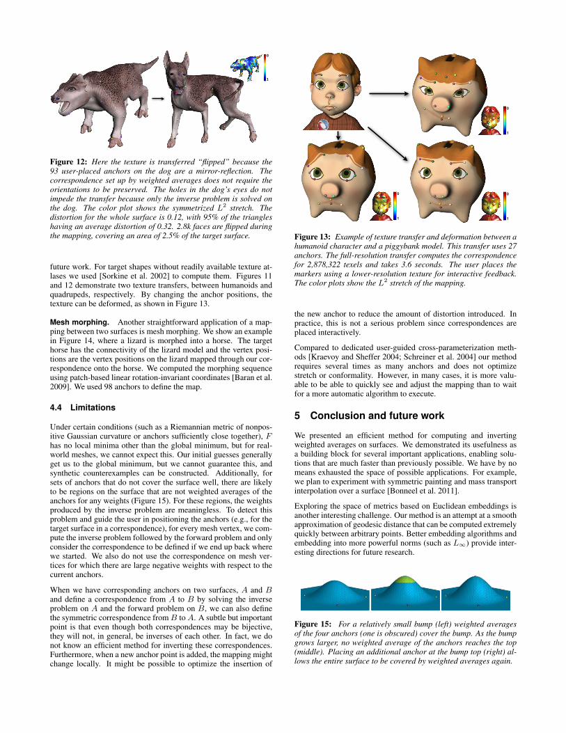
Figure 12: Here the texture is transferred “flipped” because the93 user-placed anchors on the dog are a mirror-reflection. Thecorrespondence set up by weighted averages does not require theorientations to be preserved. The holes in the dog’s eyes do notimpede the transfer because only the inverse problem is solved onthe dog. The color plot shows the symmetrized L

2 stretch. Thedistortion for the whole surface is 0.12, with 95% of the triangleshaving an average distortion of 0.32. 2.8k faces are flipped duringthe mapping, covering an area of 2.5% of the target surface.

future work. For target shapes without readily available texture at-lases we used [Sorkine et al. 2002] to compute them. Figures 11and 12 demonstrate two texture transfers, between humanoids andquadrupeds, respectively. By changing the anchor positions, thetexture can be deformed, as shown in Figure 13.

Mesh morphing. Another straightforward application of a map-ping between two surfaces is mesh morphing. We show an examplein Figure 14, where a lizard is morphed into a horse. The targethorse has the connectivity of the lizard model and the vertex posi-tions are the vertex positions on the lizard mapped through our cor-respondence onto the horse. We computed the morphing sequenceusing patch-based linear rotation-invariant coordinates [Baran et al.2009]. We used 98 anchors to define the map.

4.4 Limitations

Under certain conditions (such as a Riemannian metric of nonpos-itive Gaussian curvature or anchors sufficiently close together), Fhas no local minima other than the global minimum, but for real-world meshes, we cannot expect this. Our initial guesses generallyget us to the global minimum, but we cannot guarantee this, andsynthetic counterexamples can be constructed. Additionally, forsets of anchors that do not cover the surface well, there are likelyto be regions on the surface that are not weighted averages of theanchors for any weights (Figure 15). For these regions, the weightsproduced by the inverse problem are meaningless. To detect thisproblem and guide the user in positioning the anchors (e.g., for thetarget surface in a correspondence), for every mesh vertex, we com-pute the inverse problem followed by the forward problem and onlyconsider the correspondence to be defined if we end up back wherewe started. We also do not use the correspondence on mesh ver-tices for which there are large negative weights with respect to thecurrent anchors.

When we have corresponding anchors on two surfaces, A and B

and define a correspondence from A to B by solving the inverseproblem on A and the forward problem on B, we can also definethe symmetric correspondence from B to A. A subtle but importantpoint is that even though both correspondences may be bijective,they will not, in general, be inverses of each other. In fact, we donot know an efficient method for inverting these correspondences.Furthermore, when a new anchor point is added, the mapping mightchange locally. It might be possible to optimize the insertion of

0

1

0

1

0

1

Figure 13: Example of texture transfer and deformation between ahumanoid character and a piggybank model. This transfer uses 27anchors. The full-resolution transfer computes the correspondencefor 2,878,322 texels and takes 3.6 seconds. The user places themarkers using a lower-resolution texture for interactive feedback.The color plots show the L

2 stretch of the mapping.

the new anchor to reduce the amount of distortion introduced. Inpractice, this is not a serious problem since correspondences areplaced interactively.

Compared to dedicated user-guided cross-parameterization meth-ods [Kraevoy and Sheffer 2004; Schreiner et al. 2004] our methodrequires several times as many anchors and does not optimizestretch or conformality. However, in many cases, it is more valu-able to be able to quickly see and adjust the mapping than to waitfor a more automatic algorithm to execute.

5 Conclusion and future work

We presented an efficient method for computing and invertingweighted averages on surfaces. We demonstrated its usefulness asa building block for several important applications, enabling solu-tions that are much faster than previously possible. We have by nomeans exhausted the space of possible applications. For example,we plan to experiment with symmetric painting and mass transportinterpolation over a surface [Bonneel et al. 2011].

Exploring the space of metrics based on Euclidean embeddings isanother interesting challenge. Our method is an attempt at a smoothapproximation of geodesic distance that can be computed extremelyquickly between arbitrary points. Better embedding algorithms andembedding into more powerful norms (such as L1) provide inter-esting directions for future research.

Figure 15: For a relatively small bump (left) weighted averagesof the four anchors (one is obscured) cover the bump. As the bumpgrows larger, no weighted average of the anchors reaches the top(middle). Placing an additional anchor at the bump top (right) al-lows the entire surface to be covered by weighted averages again.

Figure 14: A morph between a lizard and a horse, using a dense correspondence computed with weighted averages. The symmetrizedL

2 stretch for the whole surface is 0.09, with 95% of the triangles having an average distortion of 0.46. 2.1k faces are flipped during themapping, covering an area of 2.6% of the target surface.

Acknowledgements

We thank the anonymous reviewers for their insightful commentsand Emily Whiting for narrating the accompanying video. The Boymodel in Figure 11 was kindly provided by Maurizio Nitti. Thiswork was supported in part by the ERC grant iModel (StG-2012-306877), by an SNF award 200021 137879 and a gift from AdobeResearch.

References

ALEXA, M. 2002. Linear combination of transformations. ACMTrans. Graph. 21, 3, 380–387.

BARAN, I., VLASIC, D., GRINSPUN, E., AND POPOVIC, J. 2009.Semantic deformation transfer. ACM Trans. Graph. 28, 3.

BONNEEL, N., VAN DE PANNE, M., PARIS, S., AND HEIDRICH,W. 2011. Displacement interpolation using lagrangian masstransport. ACM Trans. Graph. 30, 6.

BOTSCH, M., AND SORKINE, O. 2008. On linear variational sur-face deformation methods. IEEE Trans. Visualization and Com-puter Graphics 14, 1, 213–230.

BOTSCH, M., STEINBERG, S., BISCHOFF, S., AND KOBBELT, L.2002. OpenMesh - a generic and efficient polygon mesh datastructure. In Proc. OpenSG Symposium.

BOUBEKEUR, T., AND ALEXA, M. 2008. Phong tessellation.ACM Trans. Graph. 27, 5, 141:1–141:5.

BUSS, S. R., AND FILLMORE, J. P. 2001. Spherical averages andapplications to spherical splines and interpolation. ACM Trans.Graph. 20, 2, 95–126.

CARTAN, E. 1929. Groupes simples clos et ouverts et geometrieriemannienne. J. Math. Pures Appl. 8, 1–33.

CHEN, Y., AND MEDIONI, G. 1991. Object modeling by regis-tration of multiple range images. In Proc. IEEE InternationalConference on Robotics and Automation, 2724–2729.

COX, T. F., AND COX, M. A. A. 2000. Multidimensional Scaling,Second Edition. Chapman & Hall/CRC, Sept.

CRANE, K., WEISCHEDEL, C., AND WARDETZKY, M. 2013.Geodesics in heat. ACM Trans. Graph.. to appear.

DE SILVA, V., AND TENENBAUM, J. B. 2002. Global versus localmethods in nonlinear dimensionality reduction. In Proc. NIPS,705–712.

ECKSTEIN, I., SURAZHSKY, V., AND GOTSMAN, C. 2001. Tex-ture mapping with hard constraints. Comput. Graph. Forum 20,3, 95–104.

FLOATER, M. S. 2003. Mean value coordinates. Computer AidedGeometric Design 20, 1, 19–27.

FRECHET, M. 1948. Les elements aletoires de nature quelconquedans un espace distancie. Ann. Inst. H. Poincare 10, 4, 215–310.

HOFER, M., AND POTTMANN, H. 2004. Energy-minimizingsplines in manifolds. ACM Trans. Graph. 23, 3, 284–293.

HORMANN, K., AND SUKUMAR, N. 2008. Maximum entropycoordinates for arbitrary polytopes. In Proc. SGP, 1513–1520.

HORMANN, K., POLTHIER, K., AND SHEFFER, A. 2008. Meshparameterization: Theory and practice. In SIGGRAPH ASIA2008 Course Notes.

JIN, J., GARLAND, M., AND RAMOS, E. A. 2009. MLS-basedscalar fields over triangle meshes and their application in meshprocessing. In Proc. ACM I3D, 145–153.

JOSHI, P., MEYER, M., DEROSE, T., GREEN, B., ANDSANOCKI, T. 2007. Harmonic coordinates for character articu-lation. ACM Trans. Graph. 26, 3, 71:1–71:9.

JU, T., SCHAEFER, S., AND WARREN, J. 2005. Mean value coor-dinates for closed triangular meshes. ACM Trans. Graph. 24, 3,561–566.

KARCHER, H. 1977. Riemannian center of mass and mollifiersmoothing. Communications on pure and applied mathematics30, 5, 509–541.

KENDALL, W. 1990. Probability, convexity, and harmonic mapswith small image I: uniqueness and fine existence. Proceedingsof the London Mathematical Society 3, 2, 371.

KIM, V. G., LIPMAN, Y., AND FUNKHOUSER, T. 2011. Blendedintrinsic maps. ACM Trans. Graph. 30, 4.

KOBBELT, L., VORSATZ, J., AND SEIDEL, H.-P. 1999. Multires-olution hierarchies on unstructured triangle meshes. Comput.Geom. Theory Appl. 14, 1-3, 5–24.

KRAEVOY, V., AND SHEFFER, A. 2004. Cross-parameterizationand compatible remeshing of 3D models. ACM Trans. Graph.23, 3, 861–869.

LANGER, T., BELYAEV, A., AND SEIDEL, H.-P. 2006. Sphericalbarycentric coordinates. In Proc. SGP, 81–88.

LIPMAN, Y., KOPF, J., COHEN-OR, D., AND LEVIN, D. 2007.GPU-assisted positive mean value coordinates for mesh defor-mations. In Proc. SGP, 117–124.

LIPMAN, Y., RUSTAMOV, R. M., AND FUNKHOUSER, T. A.2010. Biharmonic distance. ACM Trans. Graph. 29, 3.

LOOP, C. 1987. Smooth subdivision surfaces based on triangles.Master’s thesis, Department of Mathematics, University of Utah.

OVSJANIKOV, M., MERIGOT, Q., MEMOLI, F., AND GUIBAS,L. J. 2010. One point isometric matching with the heat ker-nel. Comput. Graph. Forum 29, 5, 1555–1564.

PALFIA, M. 2009. The Riemann barycenter computation andmeans of several matrices. Int. J. Comput. Math. Sci. 3, 3, 128–133.

PENNEC, X. 1998. Computing the mean of geometric features: Ap-plication to the mean rotation. Rapport de Recherche RR–3371,INRIA - Epidaure project, Sophia Antipolis, France, March.

PHONG, B. 1975. Illumination for computer generated pictures.Communications of the ACM 18, 6, 311–317.

RITSCHEL, T., THORMAHLEN, T., DACHSBACHER, C., KAUTZ,J., AND SEIDEL, H.-P. 2010. Interactive on-surface signal de-formation. ACM Trans. Graph. 29, 4.

RUSTAMOV, R., LIPMAN, Y., AND FUNKHOUSER, T. 2009. In-terior distance using barycentric coordinates. Comput. Graph.Forum 28, 5.

RUSTAMOV, R. 2010. Barycentric coordinates on surfaces. Com-put. Graph. Forum 29, 5, 1507–1516.

SANDER, P. V., GU, X., GORTLER, S. J., HOPPE, H., AND SNY-DER, J. 2000. Silhouette clipping. In Proc. ACM SIGGRAPH,327–334.

SCHMIDT, R., GRIMM, C., AND WYVILL, B. 2006. Interactivedecal compositing with discrete exponential maps. ACM Trans.Graph. 25, 3, 605–613.

SCHREINER, J., ASIRVATHAM, A., PRAUN, E., AND HOPPE, H.2004. Inter-surface mapping. ACM Trans. Graph. 23, 3.

SETHIAN, J. A. 1996. A fast marching level set method for mono-tonically advancing fronts. In Proc. Nat. Acad. Sci, 1591–1595.

SORKINE, O., AND COHEN-OR, D. 2004. Least-squares meshes.In Proc. Shape Modeling International, 191–199.

SORKINE, O., COHEN-OR, D., GOLDENTHAL, R., ANDLISCHINSKI, D. 2002. Bounded-distortion piecewise mesh pa-rameterization. In Proc. IEEE Visualization, 355–362.

SUMNER, R. W., AND POPOVIC, J. 2004. Deformation transferfor triangle meshes. ACM Trans. Graph. 23, 3, 399–405.

SURAZHSKY, V., SURAZHSKY, T., KIRSANOV, D., GORTLER,S. J., AND HOPPE, H. 2005. Fast exact and approximategeodesics on meshes. ACM Trans. Graph. 24, 3, 553–560.

TZUR, Y., AND TAL, A. 2009. FlexiStickers: Photogrammetrictexture mapping using casual images. ACM Trans. Graph. 28, 3.

WALDRON, S. 2011. Affine generalised barycentric coordinates.Jaen Journal on Approximation 3, 2.

WALLNER, J., AND POTTMANN, H. 2006. Intrinsic subdivisionwith smooth limits for graphics and animation. ACM Trans.Graph. 25, 2, 356–374.

XIN, S.-Q., YING, X., AND HE, Y. 2012. Constant-time all-pairsgeodesic distance query on triangle meshes. In Proc. ACM I3D.

YEH, I.-C., LIN, C.-H., SORKINE, O., AND LEE, T.-Y. 2011.Template-based 3D model fitting using dual-domain relaxation.IEEE Trans. Vis. Comput. Graph. 17, 8, 1178–1190.

ZHOU, K., SYNDER, J., GUO, B., AND SHUM, H.-Y. 2004. Iso-charts: stretch-driven mesh parameterization using spectral anal-ysis. In Proc. SGP, ACM, New York, NY, USA, 45–54.